Hydrogeophysical Methods for Analyzing Aquifer Storage and Recovery Systems by Burke J. Minsley1,2, Jonathan Ajo-Franklin3, Amitabha Mukhopadhyay4, and Frank Dale Morgan2 1Corresponding author: Currently at U.S. Geological Survey, Denver Federal Center, MS964, Denver, CO

80225; (303) 236-5718; fax: (303) 236-1425; bminsley@usgs.gov 2Department of Earth, Atmospheric, and Planetary Sciences, Massachusetts Institute of Technology, 77

Massachusetts Avenue, 54-1821 Cambridge, MA 02139. 3Lawrence Berkeley National Laboratory, 1 Cyclotron Road, MS90-1116 Berkeley, CA 94720. (JAF is

partially supported under DOE-LBNL Contract No. DE-AC02-05CH11231.) 4Kuwait Institute for Scientific Research, P.O. Box 24885, 13109 Safat, Kuwait.

Abstract Hydrogeophysical methods are presented that support the siting and monitoring of aquifer storage and

recovery (ASR) systems. These methods are presented as numerical simulations in the context of a proposed ASR experiment in Kuwait, although the techniques are applicable to numerous ASR projects. Bulk geophysical properties are calculated directly from ASR flow and solute transport simulations using standard petrophysical relationships and are used to simulate the dynamic geophysical response to ASR. This strategy provides a quantitative framework for determining site-specific geophysical methods and data acquisition geometries that can provide the most useful information about the ASR implementation. An axisymmetric, coupled fluid flow and solute transport model simulates injection, storage, and withdrawal of fresh water (salinity ~500 ppm) into the Dammam aquifer, a tertiary carbonate formation with native salinity approximately 6000 ppm. Sensitivity of the flow simulations to the correlation length of aquifer heterogeneity, aquifer dispersivity, and hydraulic permeability of the confining layer are investigated. The geophysical response using electrical resistivity, time-domain electromagnetic (TEM), and seismic methods is computed at regular intervals during the ASR simulation to investigate the sensitivity of these different techniques to changes in subsurface properties. For the electrical and electromagnetic methods, fluid electric conductivity is derived from the modeled salinity and is combined with an assumed porosity model to compute a bulk electrical resistivity structure. The seismic response is computed from the porosity model and changes in effective stress due to fluid pressure variations during injection/recovery, while changes in fluid properties are introduced through Gassmann fluid substitution. Introduction

Efficient use of water resources is becoming increasingly important throughout the world due to rising demand, particularly in locations where resources are scarce and/or expensive to produce. Aquifer storage and recovery (ASR) is one method that is gaining attention as a means of storing excess water during periods when seasonal demand is less than capacity, or in the case of an emergency interruption in supply (e.g., Pyne 1995). ASR involves injecting surplus water into an existing subsurface aquifer, with the intention of withdrawing for use later when demand is high. This has certain advantages over

surface storage in tanks or reservoirs, such as reduced land use, decreased risk of contamination or tampering, and reduced loss to evaporation.

One challenge, however, is to ensure that a significant portion of stored water will be recoverable in the future. This involves understanding the dynamic hydrogeologic response of the aquifer system to artificial groundwater recharge and recovery, so that wells can be optimally sited and operated. In addition to hydrologic and geochemical data collected in observation wells, geophysical methods can provide valuable information

about subsurface structures and physical properties thatwill be useful in both the planning and monitoring phasesof an ASR program. Geophysical methods have beenused for many years in a variety of hydrogeologic appli-cations (Rubin and Hubbard 2005), although they havenot been widely applied to ASR projects. For example,Bevc and Morrison (1991) used DC resistivity to moni-tor a salt water injection experiment, Singha et al. (2007)used geoelectric measurements to study complex transportbehavior during an ASR experiment in a fractured aquifer,Darnet et al. (2004) discussed the origin of self-potentialsignals during injection into a geothermal reservoir, Daviset al. (2008) used time-lapse microgravity surveys to mon-itor aquifer storage in a coal mine, Miller et al. (2006)investigated the feasibility of using time-lapse controlledsource electromagnetic methods to monitor an aquiferstorage experiment, and Parra et al. (2006) used seismicdata to characterize subsurface aquifer properties to guidethe placement of future ASR wells.

In this study, we evaluate the utility of severalgeophysical methods in the context of a proposed ASRstudy in Kuwait (Mukhopadhyay et al. 1998). Kuwait isan arid nation with an average annual rainfall of 110 mmand negligible natural recharge from the ground surface(Mukhopadhyay et al. 1996). The average annual freshwater consumption rate in Kuwait for the year 2004 was473 L/day/capita, with a total population of nearly threemillion, met almost exclusively by desalination (Al-Otaibiand Mukhopadhyay 2005). An additional 150 L/day/capitaof brackish groundwater (3000 to 5000 mg/L) is usedprimarily for irrigation and landscaping, which is puttingsignificant stress on the groundwater reservoirs (Al-Otaibiand Mukhopadhyay 2005; Al-Senafy and Abraham 2004).One possible strategy to mitigate this problem is to usetreated waste water that is being processed at a reverseosmosis plant for irrigation and agricultural use. Theoutput of treated waste water was approximately 320,000m3/d in 2004 and is expected to double by 2025 (Al-Otaibi and Mukhopadhyay 2005). Excess treated wastewater can also be used for artificial groundwater recharge.Because of seasonal variability in demand, there was anaverage of approximately 115,000 m3/d in 2004 of excesscapacity fresh water from desalination that could also bemade available for artificial recharge.

Our goal is to understand the sensitivity of variousgeophysical techniques to the natural subsurface hydroge-ologic structure as well as changes caused by injection orwithdrawal of water into a confined aquifer, with the planthat the most useful method(s) will be used during futurefield experiments. The finite-element package COMSOLMultiphysics is used to simulate the ASR phases usinga coupled fluid flow and solute transport model. Existinghydrogeologic information about the area (Al-Awadi et al.1998; Mukhopadhyay et al. 1996), based primarily oninformation obtained from the many wells used for waterand oil production in Kuwait since the 1960s (Figure 1),is incorporated into the flow model. At any stage in thesimulation, the geophysical response can be computed

from the relevant hydrogeologic parameters such as pres-sure, salinity, density, and porosity. One benefit for boththe numerical and field experiments is that time-lapse datacan be collected. Differencing the preinjection and postin-jection datasets helps to isolate the effect of the injectionand remove background structure.

In this study, the primary geophysical response tothe ASR simulation is due to changes in the electricalresistivity structure, which is determined from variationsin aquifer salinity and the static porosity structure usingArchie’s law. We therefore focus on two methods that aresensitive to the subsurface electrical properties, DC resis-tivity and time-domain electromagnetics (TEM). Otherelectromagnetic methods, such as controlled source audiomagnetotellurics (CSAMT), may also prove useful butare not investigated here. Additionally, we investigate theseismic response to the injection experiment, which is pri-marily sensitive to changes in effective stress due to porepressure changes, but is also influenced to a small extentby changes in fluid seismic velocity due to variations insalinity.

Other geophysical techniques determined to havevery limited sensitivity to this particular ASR case studyand are therefore not considered in detail, include self-potentials and gravity. The self-potential response is verysmall (well below typical noise of a few millivolts) due tothe deep injection in this case study. Variations in gravityare far too small to be detectable in this study where fluidis injected into a confined aquifer and density changesare solely due to salinity changes rather than the case offluids displacing air in an unconfined aquifer. Methodsthat are sensitive to surface deformation, such as globalpositioning system (GPS) or interferometric syntheticaperture radar (InSAR) monitoring, have been appliedto aquifer compaction problems related to hydrocarbonproduction (e.g., Nagel 2001) and may prove useful infuture studies of large-scale ASR experiments.

Site Hydrogeology and Aquifer ModelBackground Hydrogeology

The general stratigraphy and hydrogeologic units forthe tertiary sedimentary sequence in Kuwait are shownin Figure 2. In Kuwait, useable groundwater (salinity lessthan 5000 mg/L) occurs in the aquifers of the Dammamformation and the Kuwait group. The recharge in theseaquifers from rainfall mainly takes place outside theterritory of Kuwait in Saudi Arabia and Iraq. The regionalsetting suggests that the groundwater flows from theserecharge zones toward the north and east and becomesmore saline as it reaches the discharge zone along thecoast of the Arabian Gulf. The Gulf is underlain by a staticbody of very saline water (more than 150,000 mg/L),and Kuwait is situated in the northwestern corner of thisdischarge zone.

Because of the higher salinity (a minimum of4000 mg/L), hydrogen sulfide content and low productiv-ity (transmissivity in the upper part of the aquifer around40 m2/d in the southwestern part of the country), the Umm

2 B.J. Minsley et al. GROUND WATER NGWA.org

2

Figure 1. Map of Kuwait denoting water fields (blue), oil fields (brown), and agricultural areas (green).

Er-Radhuma aquifer is not exploited in Kuwait (Omaret al. 1981). The anhydritic Rus formation and the basalshales of the lower members of the Dammam formationact as an aquitard in Kuwait, separating the underlyingUmm Er-Radhuma aquifer from the Dammam aquifer.

The lithology, petrophysical characteristics such asporosity and permeability, and distribution of lost cir-culation zones in existing wells suggest that the uppermember, and possibly the middle member constitutethe main aquifers in the Dammam formation (Al-Awadiand Mukhopadhyay 1995). Because of its karstic nature,the transmissivity in the Dammam formation is vari-able, especially in the south and southwestern parts ofKuwait, but shows a general decreasing trend toward thenortheast. The silicified topmost part of the Dammam for-mation, in conjunction with the basal shaley/clayey layersof the Kuwait group, forms an aquitard that separatesthe Dammam aquifer from the overlying Kuwait groupaquifer, although hydraulic continuity is possibly main-tained in some locations through fractures that are presentin the top part of the Dammam formation.

The undifferentiated Fars and the Ghar formationsof Kuwait constitute the main Kuwait group aquifer.A sandy-shaley unit that acts as an aquitard dividesthis aquifer into upper and lower units. The loweraquifer is semiconfined in nature, and the upper aquifer

is unconfined in the central and southern parts of thecountry. The total transmissivity of the Kuwait groupaquifer increases from southwest (less than or equal to10 m2/d) to northeast (greater than or equal to 1500 m2/d),corresponding with an increase in saturated thickness inthis direction (from 0 to 400 m).

Synthetic Aquifer Model DefinitionWe define a synthetic aquifer model, illustrated in

Figure 3, that is based on the relevant hydrogeologicunits discussed in the preceding paragraphs, with aquiferparameters taken primarily from Mukhopadhyay and Al-Otaibi (2002). This model is used to simulate the dynamichydrogeologic response of ASR, which is subsequentlyused to compute the geophysical response at variousstages during an ASR experiment. For computationalefficiency, we first consider injection and recovery usinga single well in an axisymmetric model, where thesymmetry axis lies at 0 m at the left of Figure 3. Althoughthe axisymmetric model is somewhat simplified and doesnot account for the influence of structural topographyor regional groundwater flow, it provides a usefulstep toward understanding the general hydrogeophysicalcharacteristics of the ASR experiment. Future modelingexperiments will focus on a three-dimensional (3D)geometry with multiple injection and recovery wells to

NGWA.org B.J. Minsley et al. GROUND WATER 3

3

Figure 2. General Kuwait stratigraphy and hydrogeologic units (adapted from Mukhopadhyay et al. 1996).

Figure 3. Synthetic aquifer model used for hydrogeologic and geophysical modeling (based on Mukhopadhyay and Al-Otaibi2002).

4 B.J. Minsley et al. GROUND WATER NGWA.org

4

simulate the large-scale implementation of ASR that hasbeen proposed in Kuwait (Mukhopadhyay et al. 1998).

The aquifer parameters for our baseline model aretaken from the “reference run” in Mukhopadhyay and Al-Otaibi (2002) and are summarized in Table 1. Variationson this baseline model can be used to understand thesensitivity of the hydrogeophysical response to differentparameters. In this study, we investigate the effectsof (1) varying the length of the screened portion ofthe ASR well, (2) using a heterogeneous hydraulicpermeability model within the Dammam aquifer, whichis where most of the flow occurs, (3) varying the verticalhydraulic permeability of the aquitard, and (4) varying thedispersivity within the Dammam aquifer. Mukhopadhyayand Al-Otaibi (2002) suggest that the latter two effectshave significant control on the subsurface flow behavior.

Coupled Fluid Flow and Solute TransportModelingModeling Equations

Numerical simulation of an ASR experiment requirestracking the injection of fresh water (low salinity) into a(typically) more saline aquifer, followed by storage andrecovery phases. Repeated injection-recovery cycles aresometimes used to create a buffer between the naturalaquifer and the injected water (Pyne 1995). Modeling theASR process can be accomplished by solving the coupledfluid mass balance and solute transport equations (Ackereret al. 1999; Bear 1972), where fluid salinity is the statevariable within the solute transport equation. The fluidmass balance is given by:

ρS∂P

∂t+ φ

∂ρ

∂C

∂C

∂t+ ∇(ρq) = ρQ (1)

where P (Pa) is the state variable that represents hydraulicpressure, ρ is the fluid density (kg/m3), S is the specificstorativity (1/Pa), φ is the porosity (·), C is the fluidsalinity (kg/m3), Q represents a fluid source or sink (1/s),and q is the Darcy flux (m/s) such that:

q = − kμ

∇(P + ρgz) (2)

In Equation 2, k is the hydraulic permeability tensor(m2), μ is the fluid viscosity (Pa s), g is the gravitationalacceleration (m/s2), and z is elevation (m). Solutetransport is governed by an advection-dispersion equation:

φ∂C

∂t+ ∇(−φD∇C + qC) = 0 (3)

where the fluid salinity, C, is the state variable and D isthe dispersion tensor,

D = DmI + (αL − αT)qqT

|q | + αT|q |I (4)

The dispersion tensor consists of both moleculardiffusion, Dm (m2/s), and mechanical dispersion that is

Tab

le1

Bas

elin

eA

quif

erP

aram

eter

sfo

rN

umer

ical

Mod

elin

g

Per

mea

bilit

y,k

(m2)

Dis

pers

ivit

y(m

)

Lay

erT

hick

ness

(m)

Dep

thto

Top

(m)

Hor

izon

tal

Ver

tica

lSp

ecifi

cSt

orag

e,S

(1/m

)P

oros

ity,

φL

ongi

tudi

nal,

αL

Tra

nsve

rse,

αT

Uns

atur

ated

Kuw

ait

grou

p35

0n/

an/

a0.

2n/

aTo

pK

uwai

tgr

oup

1035

2.4

×10

−13

2.4

×10

−14

0.00

018

0.2

1.0

0.1

Upp

erK

uwai

tgr

oup

2545

2.4

×10

−12

2.4

×10

−13

0.00

018

0.2

1.0

0.1

Low

erK

uwai

tgr

oup

2070

3.0

×10

−12

1.2

×10

−14

0.00

018

0.25

1.0

0.1

Aqu

itar

d30

901.

2×

10−1

31.

0×

10−1

50.

0001

80.

051.

00.

1D

amm

am80

120

1.2

×10

−12

1.2

×10

−13

5.0

×10

−60.

0510

.01.

0B

asal

Dam

mam

and

Rus

100

200

1.0

×10

−14

1.0

×10

−15

5.0

×10

−60.

031.

00.

1

NGWA.org B.J. Minsley et al. GROUND WATER 5

5

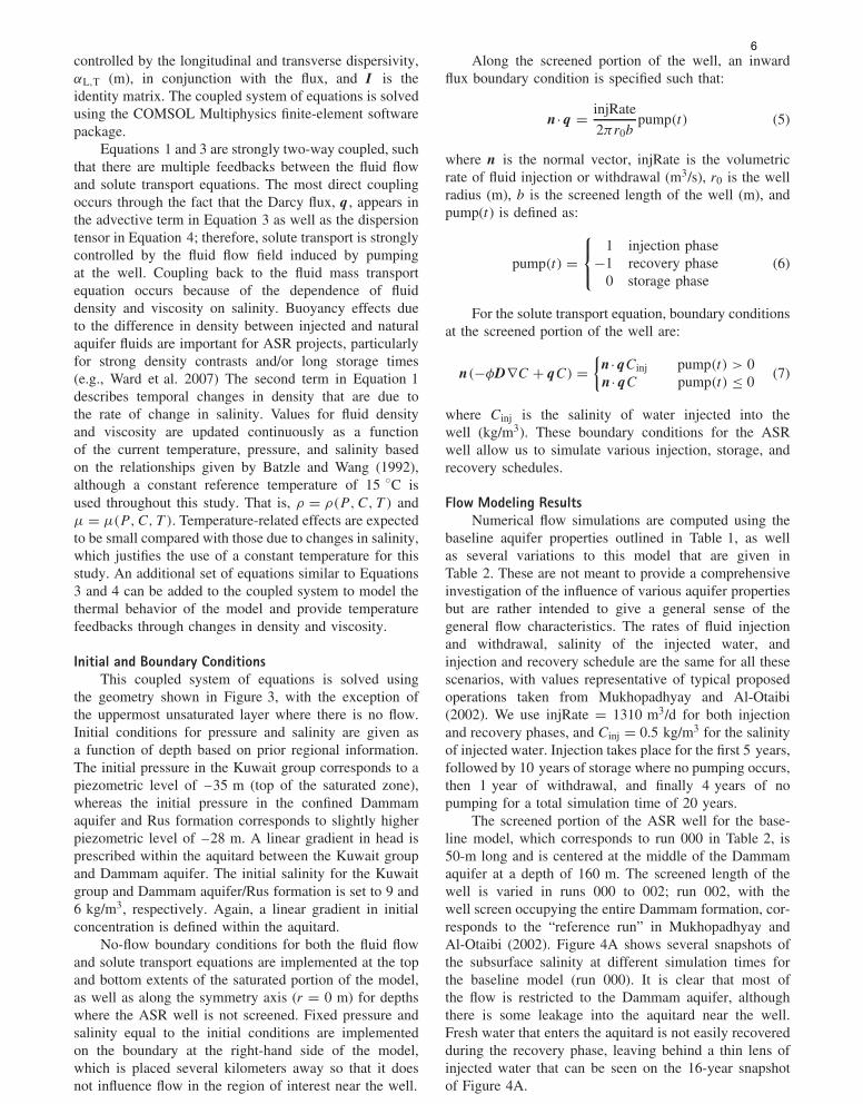
controlled by the longitudinal and transverse dispersivity,αL,T (m), in conjunction with the flux, and I is theidentity matrix. The coupled system of equations is solvedusing the COMSOL Multiphysics finite-element softwarepackage.

Equations 1 and 3 are strongly two-way coupled, suchthat there are multiple feedbacks between the fluid flowand solute transport equations. The most direct couplingoccurs through the fact that the Darcy flux, q , appears inthe advective term in Equation 3 as well as the dispersiontensor in Equation 4; therefore, solute transport is stronglycontrolled by the fluid flow field induced by pumpingat the well. Coupling back to the fluid mass transportequation occurs because of the dependence of fluiddensity and viscosity on salinity. Buoyancy effects dueto the difference in density between injected and naturalaquifer fluids are important for ASR projects, particularlyfor strong density contrasts and/or long storage times(e.g., Ward et al. 2007) The second term in Equation 1describes temporal changes in density that are due tothe rate of change in salinity. Values for fluid densityand viscosity are updated continuously as a functionof the current temperature, pressure, and salinity basedon the relationships given by Batzle and Wang (1992),although a constant reference temperature of 15 ◦C isused throughout this study. That is, ρ = ρ(P, C, T ) andμ = μ(P, C, T ). Temperature-related effects are expectedto be small compared with those due to changes in salinity,which justifies the use of a constant temperature for thisstudy. An additional set of equations similar to Equations3 and 4 can be added to the coupled system to model thethermal behavior of the model and provide temperaturefeedbacks through changes in density and viscosity.

Initial and Boundary ConditionsThis coupled system of equations is solved using

the geometry shown in Figure 3, with the exception ofthe uppermost unsaturated layer where there is no flow.Initial conditions for pressure and salinity are given asa function of depth based on prior regional information.The initial pressure in the Kuwait group corresponds to apiezometric level of –35 m (top of the saturated zone),whereas the initial pressure in the confined Dammamaquifer and Rus formation corresponds to slightly higherpiezometric level of –28 m. A linear gradient in head isprescribed within the aquitard between the Kuwait groupand Dammam aquifer. The initial salinity for the Kuwaitgroup and Dammam aquifer/Rus formation is set to 9 and6 kg/m3, respectively. Again, a linear gradient in initialconcentration is defined within the aquitard.

No-flow boundary conditions for both the fluid flowand solute transport equations are implemented at the topand bottom extents of the saturated portion of the model,as well as along the symmetry axis (r = 0 m) for depthswhere the ASR well is not screened. Fixed pressure andsalinity equal to the initial conditions are implementedon the boundary at the right-hand side of the model,which is placed several kilometers away so that it doesnot influence flow in the region of interest near the well.

Along the screened portion of the well, an inwardflux boundary condition is specified such that:

n· q = injRate

2πr0bpump(t) (5)

where n is the normal vector, injRate is the volumetricrate of fluid injection or withdrawal (m3/s), r0 is the wellradius (m), b is the screened length of the well (m), andpump(t) is defined as:

pump(t) =⎧⎨⎩

1 injection phase−1 recovery phase

0 storage phase(6)

For the solute transport equation, boundary conditionsat the screened portion of the well are:

n(−φD∇C + qC) ={

n· qCinj pump(t) > 0n· qC pump(t) ≤ 0

(7)

where Cinj is the salinity of water injected into thewell (kg/m3). These boundary conditions for the ASRwell allow us to simulate various injection, storage, andrecovery schedules.

Flow Modeling ResultsNumerical flow simulations are computed using the

baseline aquifer properties outlined in Table 1, as wellas several variations to this model that are given inTable 2. These are not meant to provide a comprehensiveinvestigation of the influence of various aquifer propertiesbut are rather intended to give a general sense of thegeneral flow characteristics. The rates of fluid injectionand withdrawal, salinity of the injected water, andinjection and recovery schedule are the same for all thesescenarios, with values representative of typical proposedoperations taken from Mukhopadhyay and Al-Otaibi(2002). We use injRate = 1310 m3/d for both injectionand recovery phases, and Cinj = 0.5 kg/m3 for the salinityof injected water. Injection takes place for the first 5 years,followed by 10 years of storage where no pumping occurs,then 1 year of withdrawal, and finally 4 years of nopumping for a total simulation time of 20 years.

The screened portion of the ASR well for the base-line model, which corresponds to run 000 in Table 2, is50-m long and is centered at the middle of the Dammamaquifer at a depth of 160 m. The screened length of thewell is varied in runs 000 to 002; run 002, with thewell screen occupying the entire Dammam formation, cor-responds to the “reference run” in Mukhopadhyay andAl-Otaibi (2002). Figure 4A shows several snapshots ofthe subsurface salinity at different simulation times forthe baseline model (run 000). It is clear that most ofthe flow is restricted to the Dammam aquifer, althoughthere is some leakage into the aquitard near the well.Fresh water that enters the aquitard is not easily recoveredduring the recovery phase, leaving behind a thin lens ofinjected water that can be seen on the 16-year snapshotof Figure 4A.

6 B.J. Minsley et al. GROUND WATER NGWA.org

6

Table 2Variations in Aquifer Parameters for Different Numerical Simulations

Correlation Lengths forDammam Permeability (m)

Multiplier for DammamDispersivity

Run NumberScreened Length

of Well, b (m) Horizontal VerticalMultiplier for Aquitard

Vertical Permeability Longitudinal, αL Transverse, αT

000 50 • • •001 25 • • •002 80 • • •003 50 500 80 • •004 50 80 80 • •005 50 500 10 • •006 50 • 0.1 •007 50 • • 0.1 0.1008 50 500 80 0.1 0.1 0.1009 50 500 10 0.1 0.1 0.1010 50 80 80 0.1 0.1 0.1

• Indicates that the baseline parameters (Table 1) were used.

Figure 4. Flow simulation snapshots of aquifer salinity for (A) the baseline model parameters (r000) and two variations onthe baseline model: (B) aquitard vertical permeability reduced by an order of magnitude (r006) and (C) dispersivity withinthe Dammam aquifer reduced by an order of magnitude (r007). For all three cases, injection occurs during years 1 to 5,followed by a storage phase from years 6 to 14, withdrawal during year 15, followed again by storage until the end of thesimulation at year 20. Black-dashed lines outline the depth range of the Dammam aquifer.

NGWA.org B.J. Minsley et al. GROUND WATER 7

7

In Figure 4B, flow modeling results are shown for thecase where the baseline model is modified by reducing theaquitard vertical permeability by an order of magnitude(run 006). This limits the amount of fluid that leaksinto the aquitard but does not significantly alter thegeneral flow characteristics. Figure 4C illustrates theeffect of reducing the baseline model longitudinal andtransverse dispersivity within the Dammam aquifer by anorder of magnitude (run 007). This results in a sharperconcentration gradient at the plume front, as well as asteeper tilt of the fresh water/saline water interface.

Buoyancy effects become dominant after year 5 whenthe injection has stopped and is evident as the character-istic tilting (Ward et al. 2007) of the fresh water front thatcan be seen on the 10- and 15-year images. Fluid with-drawal during year 16 produces several effects that can beseen in the bottom panels of Figure 4: (1) an increase inthe width of the diffuse zone between the natural aquiferand the injected fresh water and (2) less regression of thefresh water front for the fluid “trapped” in the aquitardcompared with fluid in the aquifer due to the contrastin hydraulic permeability between these units. This lat-ter effect is diminished in Figure 4B because the reducedaquitard vertical permeability decreases the amount offresh water that enters the aquitard during the injectionand storage phases.

Figure 5 illustrates the general motion of the injectedfresh water plume during different ASR phases by plottingthe center of mass computed from the differential salinityat various simulation times for the baseline model, that is:

[rcm

zcm

]=

∑i

[Ci(t) − Ci(t = 0)]

[ri

zi

]∑i

[Ci(t) − Ci(t = 0)](8)

Figure 5. Movement of the center of mass of the injectedfresh water throughout the ASR simulation for simulationsr000, r006, and r007 shown in Figure 4. The effect ofthe reduced aquitard vertical permeability (r006) is clearlyevident.

Note that this calculation is applied to a single verticalplane through the axisymmetric model; the true center ofmass always remains along the well axis. Additionally,Equation 8 assumes that a constant discretization is usedin the r- and z-directions. The background salinity beforepumping occurs, C(t = 0) , is subtracted from the salinityat each time step to isolate changes due to pumping.

Motion of the plume is mostly lateral during theinjection phase that takes place over the first 5 years,followed by primarily vertical motion during the storagephase from years 5 to 15, then lateral retreat with somevertical rise during the recovery phase between years 15and 16, and finally a return to the general storage phasetrend. The reduced aquitard vertical permeability in r006has a clear impact on the vertical motion of the plumecompared with the other two scenarios. In the case ofreduced aquifer dispersivity (r007), a slight increase invertical motion of the plume is observed in comparisonwith the baseline model.

Runs 003 to 005 investigate the influence of hydraulicpermeability heterogeneity within the Dammam aquiferusing models with different vertical and horizontal cor-relation lengths (Table 2) shown in Figure 6. Each per-meability model is generated through sequential Gaussiansimulation using the same lognormal permeability targethistogram. The lognormal distribution has mean –12 andstandard deviation 0.35, which is representative of the

Figure 6. Hydraulic permeability models with different cor-relation lengths used for numerical simulations. (A) 500 ×80 m used in runs 003 and 008, (B) 80 × 80 m used in runs004 and 010, (C) 500 × 10 m used in runs 005 and 009.

8 B.J. Minsley et al. GROUND WATER NGWA.org

8

permeability range in the Dammam aquifer reported byMukhopadhyay and Al-Otaibi (2002, Table 1). This stan-dard deviation may underrepresent the variation of perme-ability of the karst aquifer and is a focus of future work.Heterogeneous porosities are defined within the modelbased on a nonlinear mapping to the permeability valueat each location. Finally, runs 008 to 010 involve combi-nations of aquifer heterogeneity with the altered aquitardpermeability and aquifer dispersivity investigated in runs006 and 007.

The use of a two-dimensional (2D) hydraulic per-meability field within an axisymmetric model is equiva-lent to concentric tubes of constant permeability aroundthe central well, which results in radially weightedhydraulic conductance values (e.g., Langevin 2008). Thismodel properly accounts for the volumetric distribution ofinjected or recovered water but presumes that there is noflow in the angular direction (perpendicular to the r − z

plane) and is not representative of realistic flow patternsdue to 3D heterogeneity.

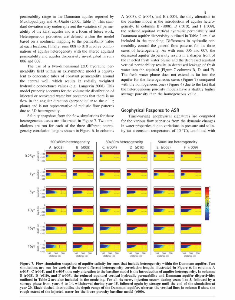
Salinity snapshots from the flow simulations for theseheterogeneous cases are illustrated in Figure 7. Two sim-ulations are run for each of the three different hetero-geneity correlation lengths shown in Figure 6. In columns

A (r003), C (r004), and E (r005), the only alteration tothe baseline model is the introduction of aquifer hetero-geneity. In columns B (r008), D (r010), and F (r009),the reduced aquitard vertical hydraulic permeability andDammam aquifer dispersivity outlined in Table 2 are alsoincluded in the modeling. Differences in hydraulic per-meability control the general flow patterns for the threecases of heterogeneity. As with runs 006 and 007, thedecreased aquifer dispersivity results in a sharper front ofthe injected fresh water plume and the decreased aquitardvertical permeability results in decreased leakage of freshwater into the aquitard (Figure 7 columns B, D, and F).The fresh water plume does not extend as far into theaquifer for the heterogeneous cases (Figure 7) comparedwith the homogeneous ones (Figure 4) due to the fact thatthe heterogeneous porosity models have a slightly higheraverage porosity than the homogeneous value.

Geophysical Response to ASRTime-varying geophysical signatures are computed

for the various flow scenarios from the dynamic changesin water properties due to variations in pressure and salin-ity (at a constant temperature of 15 ◦C), combined with

Figure 7. Flow simulation snapshots of aquifer salinity for runs that include heterogeneity within the Dammam aquifer. Twosimulations are run for each of the three different heterogeneity correlation lengths illustrated in Figure 6. In columns A(r003), C (r004), and E (r005), the only alteration to the baseline model is the introduction of aquifer heterogeneity. In columnsB (r008), D (r010), and F (r009), the reduced aquitard vertical hydraulic permeability and Dammam aquifer dispersivitiesoutlined in Table 2 are also included in the modeling. For all six cases, injection occurs during years 1 to 5, followed by astorage phase from years 6 to 14, withdrawal during year 15, followed again by storage until the end of the simulation atyear 20. Black-dashed lines outline the depth range of the Dammam aquifer, whereas the vertical lines in column B show therough extent of the injected water for the lower porosity baseline model (r000).

NGWA.org B.J. Minsley et al. GROUND WATER 9

9

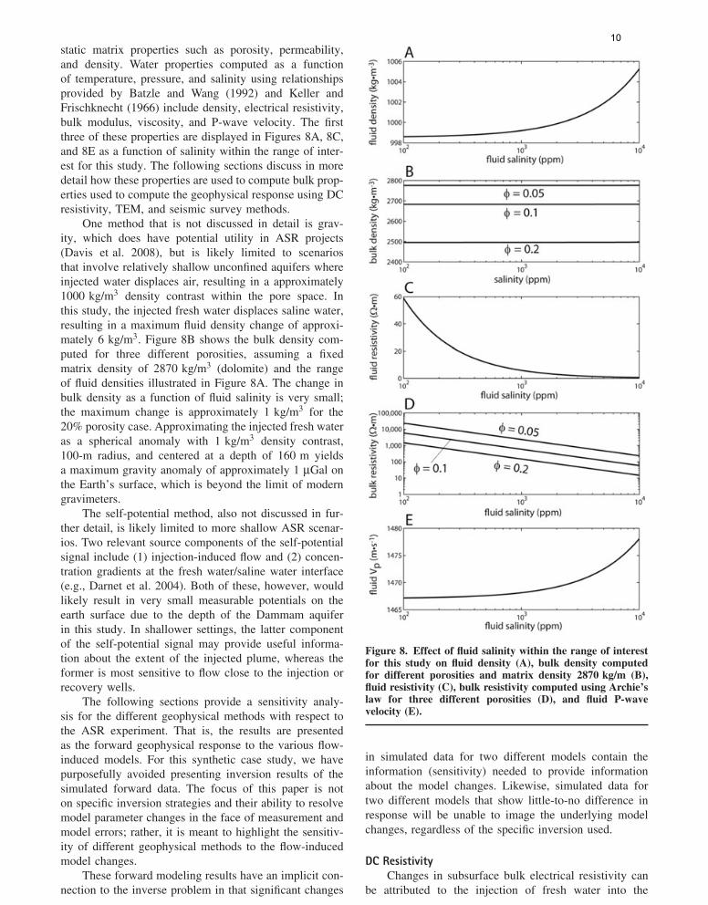
static matrix properties such as porosity, permeability,and density. Water properties computed as a functionof temperature, pressure, and salinity using relationshipsprovided by Batzle and Wang (1992) and Keller andFrischknecht (1966) include density, electrical resistivity,bulk modulus, viscosity, and P-wave velocity. The firstthree of these properties are displayed in Figures 8A, 8C,and 8E as a function of salinity within the range of inter-est for this study. The following sections discuss in moredetail how these properties are used to compute bulk prop-erties used to compute the geophysical response using DCresistivity, TEM, and seismic survey methods.

One method that is not discussed in detail is grav-ity, which does have potential utility in ASR projects(Davis et al. 2008), but is likely limited to scenariosthat involve relatively shallow unconfined aquifers whereinjected water displaces air, resulting in a approximately1000 kg/m3 density contrast within the pore space. Inthis study, the injected fresh water displaces saline water,resulting in a maximum fluid density change of approxi-mately 6 kg/m3. Figure 8B shows the bulk density com-puted for three different porosities, assuming a fixedmatrix density of 2870 kg/m3 (dolomite) and the rangeof fluid densities illustrated in Figure 8A. The change inbulk density as a function of fluid salinity is very small;the maximum change is approximately 1 kg/m3 for the20% porosity case. Approximating the injected fresh wateras a spherical anomaly with 1 kg/m3 density contrast,100-m radius, and centered at a depth of 160 m yieldsa maximum gravity anomaly of approximately 1 μGal onthe Earth’s surface, which is beyond the limit of moderngravimeters.

The self-potential method, also not discussed in fur-ther detail, is likely limited to more shallow ASR scenar-ios. Two relevant source components of the self-potentialsignal include (1) injection-induced flow and (2) concen-tration gradients at the fresh water/saline water interface(e.g., Darnet et al. 2004). Both of these, however, wouldlikely result in very small measurable potentials on theearth surface due to the depth of the Dammam aquiferin this study. In shallower settings, the latter componentof the self-potential signal may provide useful informa-tion about the extent of the injected plume, whereas theformer is most sensitive to flow close to the injection orrecovery wells.

The following sections provide a sensitivity analy-sis for the different geophysical methods with respect tothe ASR experiment. That is, the results are presentedas the forward geophysical response to the various flow-induced models. For this synthetic case study, we havepurposefully avoided presenting inversion results of thesimulated forward data. The focus of this paper is noton specific inversion strategies and their ability to resolvemodel parameter changes in the face of measurement andmodel errors; rather, it is meant to highlight the sensitiv-ity of different geophysical methods to the flow-inducedmodel changes.

These forward modeling results have an implicit con-nection to the inverse problem in that significant changes

Figure 8. Effect of fluid salinity within the range of interestfor this study on fluid density (A), bulk density computedfor different porosities and matrix density 2870 kg/m (B),fluid resistivity (C), bulk resistivity computed using Archie’slaw for three different porosities (D), and fluid P-wavevelocity (E).

in simulated data for two different models contain theinformation (sensitivity) needed to provide informationabout the model changes. Likewise, simulated data fortwo different models that show little-to-no difference inresponse will be unable to image the underlying modelchanges, regardless of the specific inversion used.

DC ResistivityChanges in subsurface bulk electrical resistivity can

be attributed to the injection of fresh water into the

10 B.J. Minsley et al. GROUND WATER NGWA.org

10

more saline Dammam aquifer. Archie’s law (Archie1942) is a commonly used relationship that relates thebulk resistivity to fluid resistivity, porosity, and watersaturation:

ρb = aρfφ−mS−n

w (9)

Here, ρb is the bulk resistivity (�·m), ρf is the fluidresistivity (�·m), ϕ is the porosity, and Sw is the fractionalwater saturation. The coefficients a, m, and n vary withrock type, but typical values are a ∼ 1, m ∼ 2, and n ∼ 2.Fluid resistivity is defined as a function of the salinity:

1/ρf = F∑

i

ui |zi |Ci (10)

where F is Faraday’s constant (96,500 C/mol) and u, z,and C are the mobility (m2/V/s), valence, and concentra-tion (kg/m3) of the ith ionic species, respectively. In thisstudy, the bulk resistivity is therefore determined primar-ily by the model porosity defined for the flow simulationsand the dynamic aquifer salinity (e.g., Figures 4 and 7).Sw increases linearly in the unsaturated Kuwait group untilit reaches 1 in the top Kuwait group. The influence of fluidsalinity on the fluid resistivity (Figure 8C) and bulk resis-tivity (Figure 8D) is illustrated for the range of salinitiesused in this study (approximately 0.1 to 9 kg/m3).

Figure 9 shows snapshots of the bulk electrical resis-tivity computed from the flow simulations for runs 000,003, and 008 using Equations 9 and 10. The resistivitystructure is clearly controlled by the distribution of fluidsalinity, although the influence of porosity is also evident.

Figure 9. Snapshots of bulk electrical resistivity computed from the flow simulations for (A) the baseline model parameters(r000) and two variations on the baseline model: (B) heterogeneity within the Dammam aquifer with correlation length 500 ×80 m (r003) and (C) reduced aquitard vertical permeability and aquifer dispersivity in addition to the aquifer heterogeneity(r008).

NGWA.org B.J. Minsley et al. GROUND WATER 11

11

For example, the higher aquitard vertical permeability inFigure 9B compared with Figure 9C results in relativelymore flow in to the low-porosity aquitard. The combi-nation of reduced salinity and porosity results in furtherincreases in electrical resistivity within the aquitard. Thesethree cases are used to illustrate changes in the predictedDC resistivity response with time, as well as differencesdue to the different modeling cases at a given simulationtime.

The DC resistivity response is simulated using a 3Dmodel that is generated by revolving the bulk resistiv-ity images in Figure 9 about a vertical axis through theorigin. The modeled data consist of a single 2D pro-file across the center of the model using an inverseWenner-Schlumberger array with 50 electrodes, eachseparated by 40 m (a-spacing). Simulated data are com-puted using a code that is based on the transmissionnetwork approach discussed by Zhang et al. (1995) andShi (1998). Changes in the modeled response are pre-sented as differential apparent resistivity pseudosections,where the apparent resistivity is given by the product ofthe geometric factor, K = πa(n + 1)n (m), with the ratioof the measured potential difference to the injected cur-rent, V /I (�).

ρa = KV

I(11)

Differential apparent resistivities are simply the point-by-point percent differences between any two pseudosections.

Time-lapse changes in apparent resistivity for caser000 are illustrated in Figures 10A and 10B. Figure 10Adisplays the total percent change in apparent resistivity foreach simulation time with respect to the preinjection state,whereas Figure 10B illustrates the incremental change inapparent resistivity between neighboring simulation times.This comparison is repeated for r003 (Figures 10C and10D) and r008 (Figures 10E and 10F). In all the cases,outward progression of the fresh water plume is evident asincreased apparent resistivity during the injection phase.This is followed by a more subtle increase in resistivityassociated with the upward and outward movement of thefresh water under its buoyancy during the storage phase.Slight decreases in apparent resistivity are observed afterthe recovery phase, as seen in the bottom pseudosectionsin Figures 10B, 10D, and 10F.

Figure 11 shows the differences in modeled apparentresistivity (%) for the different flow scenarios in Figure 9.The differences between the baseline model (r000) and thecase with 500 × 80–m aquifer heterogeneity and elevatedaquitard permeability and aquifer dispersivity (r003) areillustrated in Figure 11A. Much of the large (∼50%)difference between these cases comes from the differencein background resistivity of the Dammam aquifer for thehomogeneous and heterogeneous models, although theinfluence of the injected fresh water is also evident overthe various time steps. Figure 11B shows the apparentresistivity changes between the two heterogeneous aquifercases from Figure 9 (r003 and r008), which only differ intheir aquitard permeability and aquifer dispersivity, and

Figure 10. Time-lapse differential apparent resistivity (%) pseudosections for cases r000 (A and B), r003 (C and D), and r008(E and F). For each modeling scenario, the total differences at each time step are shown with respect to the preinjectionstate (A, C, and E) as well as incremental changes with respect to the previous simulation time step (B, D, and F). Note thatdifferent color scales are used for each column.

12 B.J. Minsley et al. GROUND WATER NGWA.org

12

Figure 11. Differential apparent resistivity (%) pseudosections between the models illustrated in Figure 9 at various simulationtimes. (A) r000 vs. r003, and (B) r008 vs. r003. Differences highlight the changes in flow patterns between different models.Note that the changes in (A) are much larger than those in (B).

therefore their flow characteristics. During the injectionphase, r008 exhibits a slightly higher (∼2%) apparentresistivity than r003 due to the greater distance that thefresh water has migrated into the aquifer (Figure 9), whichis apparent in Figure 11B. From year 5 onward, thereis also a decrease in the apparent resistivity of r008relative to r003 in the center of the pseudosection. This isattributed to the decrease in fresh water moving upwardthrough the aquitard in case r008, which has reducedvertical aquitard permeability.

There are many possible apparent resistivity compar-isons to make between the different flow simulations atvarious time steps. The purpose of the relatively smallsubset of examples provided here is to give the readera sense of the magnitudes and characteristics of thesechanges, which is representative of the various flow sim-ulations in this study. This forward modeling exercise ismeant to illustrate the sensitivity of DC resistivity mea-surements to changes in subsurface flow patterns relatedto the ASR experiment. One still needs to consider theresolution to which these flow patterns can be resolvedin an inversion given these data and their geometry, aswell as noise that can be expected to be recorded in thefield.

Time-Domain Electromagnetics (TEM)TEM soundings provide another means for char-

acterizing the subsurface electrical resistivity structureand have been used previously in numerous hydrogeo-logic studies (e.g., Auken et al. 2006; Danielsen et al.2003; Fitterman and Stewart 1986). In contrast with thegalvanically coupled DC resistivity method, TEM is aninductive technique, which may provide some practicaladvantage over DC resistivity in the desert environmentwhere high electrode contact resistances can be an issue(Al-Ruwaih and Ali 1986). The basic principle involvespassing a constant current through a loop of wire on theEarth’s surface, which produces a primary magnetic field.This current is then rapidly turned off, inducing a ringof horizontal currents in the subsurface that immediatelymaintain the initial magnetic field. The current systemsubsequently decays as it diffuses downward through thesubsurface resistivity structure, producing a time-varyingsecondary magnetic field that is recorded by a receivingcoil on the surface.

The TEM response is computed from the same bulkresistivity models used for the DC resistivity example inthe previous section, although we are currently restrictedto the one-dimensional (1D) forward modeling code,EMMA (Auken et al. 2002). Because of the inherently

NGWA.org B.J. Minsley et al. GROUND WATER 13

13

3D character of the injected fresh water “bubble,” this1D forward modeling exercise is somewhat limited,particularly for early simulation times when the lateralextent of the injected fresh water is relatively smallcompared with the aquifer depth. This is due to the natureof the increasing volume of sensitivity as the inducedcurrent system diffuses downward through the earthstructure (Nabighian and Macnae 1991), sampling boththe background resistivity structure and the anomalousvolume. By extracting 1D resistivity profiles from thecenter of the axisymmetric models, we are effectivelyinvestigating the maximum observable TEM response,when the extent of the injected fresh water is much largerthan the dimension of the transmitting loop.

Although smaller transmitter loops can be used toimprove lateral resolution, the signal strength (and there-fore depth of investigation) depends on the transmittermoment, proportional to the product of the transmittingloop area and the current in the loop. Therefore, to achievethe same moment as a 100-m rectangular loop with 10 Aof current, a 25-m loop would require 160 A of current,which is well beyond the capability of commercial TEMsystems. For the current study, the TEM response is sim-ulated using a 100-m square transmitting loop with 25 A,and a vertically oriented receiving coil at the center ofthe transmitter. The output data are presented as dB/dt

(V/m2) decay curves, which are also converted to appar-ent resistivities. Error bars on these figures result from thedefault EMMA noise function that is applied to the data,

which has a magnitude of 2.5 × 10−9 V/m2 at 1 ms anda slope of –0.5 (i.e., the noise decays as t−0.5).

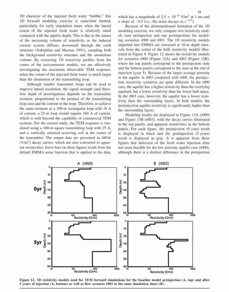
Because of the aforementioned limitation of the 1Dmodeling exercise, we only compare two resistivity mod-els (one preinjection and one postinjection) for model-ing scenarios r000 and r003. The 1D resistivity modelsimported into EMMA are extracted at 10-m depth inter-vals from the center of the bulk resistivity models illus-trated in Figure 9. Figure 12 shows the resistivity modelsfor scenarios r000 (Figure 12A) and r003 (Figure 12B),where the top panels correspond to the preinjection stateand the bottom panels correspond to the state at the end ofinjection (year 5). Because of the larger average porosityin the aquifer in r003 compared with r000, the preinjec-tion resistivity scenarios are quite different. In the r000case, the aquifer has a higher resistivity than the overlyingaquitard, but a lower resistivity than the lower half-space.In the r003 case, however, the aquifer has a lower resis-tivity than the surrounding layers. In both models, thepostinjection aquifer resistivity is significantly higher thanthe surrounding layers.

Modeling results are displayed in Figure 13A (r000)and Figure 13B (r003), with the decay curves illustratedin the top panels, and apparent resistivities in the bottompanels. For each figure, the preinjection (0 year) resultis displayed in black and the postinjection (5 years)result is displayed in gray. It is apparent from thesefigures that detection of the fresh water injection doesnot seem feasible for the low-porosity aquifer case (r000),although there is a distinct difference in the preinjection

Figure 12. 1D resistivity models used for TEM forward simulations for the baseline model preinjection (A, top) and after5 years of injection (A, bottom) as well as flow scenario r003 at the same simulation times (B).

14 B.J. Minsley et al. GROUND WATER NGWA.org

14

Figure 13. TEM results for the resistivity models shown in Figure 12. Results for the baseline model, r000 (A) are displayedas dB /dt (V/m2) (top) and apparent resistivity (�·m) (bottom). (B) Corresponding results for flow scenario r003. In all figures,the preinjection values are displayed in black, and the postinjection (year 5) results are in gray.

and postinjection TEM responses for the higher porosityaquifer case (r003). This can be attributed to the inherentdifficulty in distinguishing resistive targets compared withconductive ones (Fitterman and Stewart 1986). In the r000case, the intermediate preinjection aquifer resistivity isreplaced with a high-resistivity layer, making it difficultto detect. For the r003 case, however, the initial aquiferresistivity is relatively low, making it a good TEM targetin contrast with the postinjection resistivity.

A Seismic Monitoring StrategyIn addition to techniques based on electrical and

electromagnetic contrasts, seismic methods offer anotherpossible avenue for monitoring ASR. The primary sub-surface processes of relevance are changes in fluid mod-ulus and density due to salinity and temperature changes,and variations in effective stress due to pumping-inducedchanges in pore pressure. Effective stress variations pro-duce the dominant seismic signature in the context of anASR experiment, suggesting that seismic methods mightbe most useful in constraining pore pressure distribution

rather than the injected zone of fresh water. This modelinginvestigation focuses on vertical seismic profiling due toreported technical difficulties in obtaining high-qualitysurface seismic data on the unconsolidated sands at thestudy area. For simplicity, we only consider P-wave prop-erty variations and acoustic rather than elastic modelingalthough some additional information might be gainedthrough multicomponent surveys.

For our seismic forward modeling experiment, weconsider only scenario r003 and use the same unit des-ignations and porosities described in the flow modelingsequence. Figure 14A depicts a map of Vp over the mod-eling domain at time zero (preinjection). Velocities inour seismic model vary from 900 m/s in the unsatu-rated near-surface gravel layer to 5210 m/s in the basalDammam/Rus. Intermediate sandstone velocities are esti-mated from general literature values tabulated in Mavkoet al. (1998). Velocities for the shaly aquitard are pre-sumed using Castagna’s mudrock relationship (Castagnaet al. 1985). Properties for the Dammam itself are cal-culated using a modified Voigt + critical porosity model

NGWA.org B.J. Minsley et al. GROUND WATER 15

15

Figure 14. (A) Preinjection velocity model for flow scenario r003, with source location for the near-offset VSP denoted bythe red circle and downhole receiver array (blue line). (B) Shot gather for the baseline model generated by a 150 Hz Rickerwavelet with the primary transmission arrival is outlined in red, and basal reflection in blue.

calibrated to the Nur/Simmons Bedford limestone dataset(Supporting Information). An important caveat is thatnone of these values are calibrated to either local fielddata or measurements from the same geological unitsat a remote site; the included velocities should only beconsidered rough estimates included for the purpose ofsensitivity calculations until more reliable data becomeavailable. To convert the r003 sequence of flow results intoseismic properties, all units except for the Dammam areassumed to remain unchanged. Within the Dammam, theframe model and Gassmann fluid substitution discussedin the online Supporting Information are used to estimateproperty changes due to variations in fluid characteristics(modulus and density) as well as pore pressure.

In modeling the site’s seismic response, we considera near-offset vertical seismic profile, one of the mostcommon type of downhole seismic surveys acquiredduring monitoring activities. Because spatial sensitivityto localized variations in properties is relevant, we use2D full wavefield acoustic finite-difference (FD) modelingto estimate the response to pumping activities. The codedeveloped for this task is an explicit time-domain FDsolver (eighth order in space, second order in time) similarto the classical scheme described in Dablain (1986) withthe sponge absorbing boundary condition developed byCerjan et al. (1985).

Figure 14A depicts the source position used for thenear-offset modeling simulation (red circle) in additionto the receiver array, assumed to be in a well close tothe origin of the radial flow model. The offset betweenthe source and the receiver well is 7 m laterally andthe 200 receivers have a vertical spacing of 1.43 m.Figure 14B shows a corresponding shot gather for thebaseline model generated by a 150 Hz Ricker wavelet

with the primary transmission arrival outlined in red.As expected, the most visible velocity changes in thebackground model, visible as variations in the slope ofthe primary arrival, are the transition between the shal-low unsaturated gravel unit and the upper Kuwait groupand the transition between the Damman and the BasalDammam/Rus. Several strong reflections are also visiblewith the most dominant corresponding to the precedingtransitions. The basal Dammam/Rus reflection, outlined inblue, is probably the most useful reflection event for mon-itoring lateral variations in aquifer properties as it samplesvelocity changes across the aquifer.

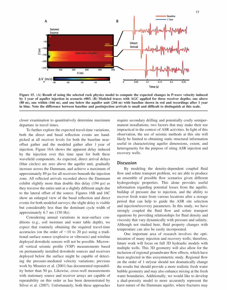
Figure 15A shows the result of using the selectedrock physics model to compute the expected changes inP-wave velocity induced by 1 year of aquifer injectionin scenario r003, the point of maximum departure fromthe initial state. A crucial observation is that the zonethat experiences significant increases in pore pressureand corresponding decreases in Vp is highly localizedwithin the vicinity of the injection well. Although peakvelocity changes near the well are –55 m/s, at a 100-moffset velocity departures are on the order of –10 m/s, achange of only approximately 0.3% from baseline levels.Although aquifer heterogeneity does induce vertical andlateral variations in the P-wave properties, the time-lapse signature is largely dominated by the distancefrom the injector. Figure 15B depicts modeled traceswith automatic gain control (AGC) applied for threereceiver depths; one above (80 m), one within (166 m),and one below the aquifer unit (244 m) with baselineshown in red and recordings after 1 year in blue. As canclearly be seen, the phase and amplitude of the modeledsignal change only a small amount in both the directand reflected components of the waveform, motivating a

16 B.J. Minsley et al. GROUND WATER NGWA.org

16

Figure 15. (A) Result of using the selected rock physics model to compute the expected changes in P-wave velocity inducedby 1 year of aquifer injection in scenario r003. (B) Modeled traces with AGC applied for three receiver depths; one above(80 m), one within (166 m), and one below the aquifer unit (244 m) with baseline shown in red and recordings after 1 yearin blue. Note the difference between baseline and postinjection arrivals is small and difficult to distinguish at this scale.

closer examination to quantitatively determine maximumdeparture in travel times.

To further explore the expected travel-time variations,both the direct and basal reflection events are hand-picked at all receiver levels for both the baseline near-offset gather and the modeled gather after 1 year ofinjection. Figure 16A shows the apparent delay inducedby the injection over this time span for both thesewavefield components. As expected, direct arrival delays(blue circles) are zero above the aquifer unit, graduallyincrease across the Dammam, and achieve a maximum ofapproximately 89 μs for all receivers beneath the injectionzone. All reflected arrivals recorded above the Dammamexhibit slightly more than double this delay (194 μs) asthey traverse the entire unit at a slightly different angle dueto the lateral offset of the source. Figures 16B and 16Cshow an enlarged view of the basal reflection and directevents for both modeled surveys; the slight delay is visiblebut considerably less than the dominant cycle width ofapproximately 6.7 ms (150 Hz).

Considering annual variations in near-surface con-ditions (e.g., soil moisture and water table depth), weexpect that routinely obtaining the required travel-timeaccuracies (on the order of ∼10 to 20 μs) using a tradi-tional surface source (explosive or vibroseis) and wirelinedeployed downhole sensors will not be possible. Microw-ell vertical seismic profile (VSP) measurements basedon permanently installed downhole sources and receiversdeployed below the surface might be capable of detect-ing the pressure-mediated velocity variations; previouswork by Meunier et al. (2001) has documented repeatabil-ity better than 50 μs. Likewise, cross-well measurementswith stationary source and receiver arrays are capable ofrepeatability on this order as has been demonstrated bySilver et al. (2007). Unfortunately, both these approaches

require secondary drilling and potentially costly semiper-manent installations, two factors that may make their useimpractical in the context of ASR activities. In light of thisobservation, the use of seismic methods at this site willlikely be limited to obtaining static structural informationuseful in characterizing aquifer dimensions, extent, andheterogeneity for the purpose of siting ASR injection andrecovery wells.

DiscussionBy modeling the density-dependent coupled fluid

flow and solute transport problem, we are able to producean ensemble of possible flow scenarios given differenthydrogeologic properties. This alone provides usefulinformation regarding potential losses from the aquifer,buildup of pressure due to injection, and the ability torecover fresh water from various locations after a storageperiod that can help to guide the ASR site selectionand injection/recovery parameters. In this study, we havestrongly coupled the fluid flow and solute transportequations by providing relationships for fluid density andviscosity that vary dynamically with pressure and salinity.Although not studied here, fluid property changes withtemperature can also be easily incorporated.

One important area of research involves the opti-mization of many injection and recovery wells; therefore,future work will focus on full 3D hydraulic models withmultiple wells. This 3D geometry will also allow for theinclusion of regional groundwater flow effects, which havebeen neglected in this axisymmetric study. Regional flowon the order of 1 m/year should not dramatically changethe results but should provide a more realistic fresh waterbubble geometry and may also enhance mixing at the freshwater boundaries. Additionally, we would like to developa dual-porosity model to more accurately represent thekarst nature of the Dammam aquifer, where fractures may

NGWA.org B.J. Minsley et al. GROUND WATER 17

17

Figure 16. (A) Apparent delay induced by 1 year of injection for both direct (blue circle) and reflected (red triangle) wavefieldcomponents. An enlarged view of the basal reflection (B) and direct events (C) for both modeled surveys highlights the smalldelays due to injection.

play a significant role in fluid transport and rate-limitedmass transfer (e.g., Culkin et al. 2008; Singha et al. 2007).

Geophysical methods represent a viable means formonitoring the various phases of an ASR project, althoughit is important to understand the expected response todifferent injection and recovery scenarios. This informa-tion will play an important role in the determination ofwhich geophysical methods should be deployed, as wellas survey design parameters. We have attempted to main-tain self-consistency throughout the modeling experimentby converting the fixed matrix and dynamic fluid proper-ties to bulk geophysical properties through various rockphysics relationships. Site-specific information to improvethe calibration of these relationships should be incorpo-rated wherever possible.

One general observation regarding the differencesbetween the electrical/electromagnetic and seismic meth-ods is that they are sensitive to different components of theflow and solute transport model. The seismic response ismainly sensitive to changes in effective stress due to porepressure changes and is therefore primarily influenced bydiffusion of pressure into the aquifer governed by the fluidmass transport equation. The electrical/electromagneticresponse, however, is mainly controlled by salinitychanges brought about by the advective flux of fresh waterinto the aquifer governed by the solute transport equation.These are complementary methods in that they can answerdifferent questions regarding the state of the aquifer dur-ing an ASR project, although we have seen that seismic

methods have relatively low sensitivity given the hydro-geologic setting of this particular study. Acquisition andcoupled inversion of multiple (time-lapse) datatypes mayprovide greater insight into the transport and storage prop-erties of the aquifer than individual methods.

There is clearly a limited response for the TEM andseismic methods, which is primarily brought about bythe particular details of this case study. The two greatestchallenges for this ASR study are (1) the relativelydeep aquifer used for injection and (2) the fact that theaquifer is confined. Many other ASR studies involveshallower, unconfined aquifers where fluids replace air inthe pore space, thereby making them a more substantialgeophysical target.

ConclusionsThe primary contribution of this modeling study

is the development of an integrated hydrogeophysicalmethodology that can be applied to a wide variety of ASRsystems and hydrogeologic settings. This work providesa framework for guiding decisions regarding the siting,operation, and monitoring of the project to ensure optimalrecovery of the stored water. The particular details of thiscase study involving a relatively deep/confined aquifer inKuwait present a challenge for geophysical monitoringmethods, and highlight the need for careful considerationand design of monitoring strategies depending on thehydrogeologic scenario.

18 B.J. Minsley et al. GROUND WATER NGWA.org

18

There are several areas for future research andimprovement on both the hydrogeologic and geophysicalaspects of this study. On the hydrogeologic side, mod-els should incorporate additional site-specific informa-tion such as layer topography and porosity-permeabilityrelationships. A dual-porosity model should also be con-sidered where fracture flow may play an important rolein flow and solute transport behavior. Additionally, afully 3D model will allow the incorporation of regionalgroundwater flow effects and the ability to study anarray of injection and recovery wells. On the geophysicalside, incorporating site-specific information to calibraterock physics relationships is an important step towardachieving more accurate modeling results. Other con-trolled source electromagnetic methods, such as airborneEM, should also be investigated, particularly for monitor-ing large study areas. Future field investigations are alsoneeded to confirm the feasibility of various geophysicalmethods for monitoring ASR.

Integrated hydrogeophysical inversion methods,which incorporate both hydrogeologic and geophysicaldatasets, will play an important role in the ability toresolve subsurface changes related to the ASR experiment.Information gained during the forward modeling analy-sis, such as presented in this study, can be used withinthe inverse process. For example, regularization strate-gies derived from the properties of the coupled flow andtransport modeling may help to produce more meaningfulhydrogeophysical inverse models.

AcknowledgmentsThis work was funded by the Kuwait-MIT Center

for Natural Resources and the Environment, with supportfrom the Kuwait Foundation for the Advancement ofScience. We are grateful for valuable suggestions providedby reviewers Fred Day-Lewis, Paul Bedrosian, WilliamHutchings, Dave Hart, and Joe Hughes.

Supporting InformationAdditional Supporting Information may be found in

the online version of this article:

This includes a seismic rock physics model forcarbonates at low effective stress levels that is used toderive the seismic modeling parameters in this study.

Please note: Wiley-Blackwell is not responsible forthe content or functionality of any supporting informationsupplied by the authors. Any queries (other than missingmaterial) should be directed to the corresponding authorfor the article.

ReferencesAckerer, P., A. Younes, and R. Mose. 1999. Modeling variable

density flow and solute transport in porous medium: 1.Numerical model and verification. Transport in PorousMedia 35, no. 3: 345–373.

Al-Awadi, E.A., and A. Mukhopadhyay. 1995. Hydrogeology ofthe Dammam formation in Umm Gudair area, Kuwait. InInternational Conference on Water Resources Managementin Arid Countries , Muscat, Sultanate of Oman.

Al-Awadi, E., A. Mukhopadhyay, and M.N. Al-Senafy. 1998.Geology and hydrogeology of the Dammam formation inKuwait. Hydrogeology Journal 6, no. 2: 302–314.

Al-Otaibi, M., and A. Mukhopadhyay. 2005. Options for manag-ing water resources in Kuwait. Arabian Journal for Scienceand Engineering 30, no. 2C: 55–68.

Al-Ruwaih, F., and H.O. Ali. 1986. Resistivity measurementsfor groundwater investigation in the Umm Al-Aish areaof northern Kuwait. Journal of Hydrology 88, no. 1–2:185–198.

Al-Senafy, M., and J. Abraham. 2004. Vulnerability of ground-water resources from agricultural activities in southernKuwait. Agricultural Water Management 64, no. 1: 1–15.

Archie, G.E. 1942. The electrical resistivity log as an aid indetermining some reservoir characteristics. Transactionsof the American Institute of Mining, Metallurgical andPetroleum Engineers 146: 54–62.

Auken, E., L. Nebel, and K.I. Sørensen. 2002. EMMA: Ageophysical training and education tool for electromagneticmodeling and analysis. Journal of Environmental andEngineering Geophysics 7: 57–68.

Auken, E., L. Pellerin, N.B. Christensen, and K. Sørensen.2006. A survey of current trends in near-surface electri-cal and electromagnetic methods. Geophysics 71, no. 5:G249–G260.

Batzle, M., and Z.J. Wang. 1992. Seismic properties of porefluids. Geophysics 57, no. 11: 1396–1408.

Bear, J. 1972. Dynamics of Fluids in Porous Media . New York:American Elsevier Pub. Co.

Bevc, D., and H.F. Morrison. 1991. Borehole-to-surface elec-trical-resistivity monitoring of a salt-water injection exper-iment. Geophysics 56, no. 6: 769–777.

Castagna, J.P., M.L. Batzle, and R.L. Eastwood. 1985. Relation-ships between compressional-wave and shear-wave veloci-ties in clastic silicate rocks. Geophysics 50: 571–581.

Cerjan, C., D. Kosloff, R. Kosloff, and M. Reshef. 1985. Anonreflecting boundary condition for discrete acoustic andelastic wave equations. Geophysics 50, no. 4: 705–708.

Culkin, S.L., K. Singha, and F.D. Day-Lewis. 2008. Implica-tions of rate-limited mass transfer for aquifer storage andrecovery. Ground Water 46, no. 4: 591–605.

Dablain, M. 1986. The application of high-order differencing tothe scalar wave equation. Geophysics 51, no. 1: 127–139.

Danielsen, J.E., E. Auken, F. Jørgensen, V. Søndergaard, andK.I. Sørensen. 2003. The application of the transient elec-tromagnetic method in hydrogeophysical surveys. Journalof Applied Geophysics 53, no. 4: 181–198.

Darnet, M., A. Maineult, and G. Marquis. 2004. On the originsof self-potential (SP) anomalies induced by water injectionsinto geothermal reservoirs. Geophysical Research Letters31, no. 19: L19609.

Davis, K., Y. Li, and M. Batzle. 2008. Time-lapse gravitymonitoring: a systematic 4D approach with applicationto aquifer storage and recovery. Geophysics 73, no. 6:WA61–WA69.

Fitterman, D.V., and M.T. Stewart. 1986. Transient electromag-netic sounding for groundwater. Geophysics 51, no. 4:995–1005.

Keller, G.V., and F.C. Frischknecht. 1966. Electrical Methodsin Geophysical Prospecting . Oxford, UK: Pergamon Press.

Langevin, C.D. 2008. Modeling axisymmetric flow and trans-port. Ground Water 46, no. 4: 579–590.

Mavko, G., T. Mukerji, and J. Dvorkin. 1998. The Rock PhysicsHandbook: Tools for Seismic Analysis in Porous Media.Cambridge, UK: Cambridge University Press.

NGWA.org B.J. Minsley et al. GROUND WATER 19

19

Meunier, J., F. Huguet, and P. Meynier. 2001. Reservoir moni-toring using permanent sources and vertical receiver anten-nae: the Cere-la-Ronde case study. The Leading Edge 6:622–629.

Miller, C., P. Routh, P. Donaldson, Y.G. Li, and D. Oldenburg.2006. Feasibility study of time-lapse controlled-source elec-tromagnetics for the aquifer storage problem. SEG Sum-mer Research Workshop on Hydrogeophysics, Vancouver,Canada.

Mukhopadhyay, A., and M. Al-Otaibi. 2002. Numerical simu-lation of freshwater storage in the Dammam formation,Kuwait. Arabian Journal for Science and Engineering 27,no. 2B: 127–150.

Mukhopadhyay, A., J. Al-Sulaimi, E. Al-Awadi, and F. Al-Ruwaih. 1996. An overview of the tertiary geology andhydrogeology of the northern part of the Arabian Gulfregion with special reference to Kuwait. Earth ScienceReviews 40, no. 3–4: 259–295.

Mukhopadhyay, A., J. Al-Sulaimi, and A.A. Al-Sumait. 1998.Creation of potable water reserves in Kuwait throughartifical recharge. In: Proceedings of the Third Inter-national Symposium on Artificial Recharge of Ground-water—TISAR98. Artificial Recharge of Groundwater ,ed. J.H. Peters, 175–180. Rotterdam, Netherlands: A.A.Balkema.

Nabighian, M.N., and J.C. Macnae. 1991. Time domain elec-tromagnetic prospecting methods. In: ElectromagneticMethods in Applied Geophysics. Application , vol. 2, ed.M.N. Nabighian. Tulsa, Oklahoma: Society of ExplorationGeophysicists.

Nagel, N.B. 2001. Compaction and subsidence issues withinthe petroleum industry: from wilmington to ekofisk and

beyond. Physics and Chemistry of the Earth, Part A: SolidEarth and Geodesy 26, no. 1–2: 3–14.

Omar, S.A., A. Al-Yacoubi, and Y. Senay. 1981. Geology andgroundwater hydrology of the State of Kuwait. Journal ofArabian Peninsula Studies 1: 5–67.

Parra, J.O., C.L. Hackert, and M.W. Bennett. 2006. Permeabilityand porosity images based on P-wave surface seismic data:application to a south Florida aquifer. Water ResourcesResearch 42, W02415.

Pyne, R.D.G. 1995. Groundwater Recharge and Wells: A Guideto Aquifer Storage Recovery . Boca Raton, Florida: LewisPublishers.

Rubin, Y., and S.S. Hubbard, ed. 2005. Hydrogeophysics. WaterScience and Technology Library; vol. 50. Dordrecht,Netherlands: Springer.

Shi, W. 1998. Advanced modeling and inversion techniquesfor three-dimensional geoelectrical surveys. Ph.D. thesis,Massachusetts Institute of Technology, Cambridge, Mas-sachusetts.

Silver, P.G., T.M. Daley, F. Niu, and E.L. Majer. 2007. Activesource monitoring of cross-well seismic travel time forstress-induced changes. Bulletin of the Seismological Soci-ety of America 97, no. 1B: 281–293.

Singha, K., F.D. Day-Lewis, and J.W. Lane Jr. 2007. Geoelec-trical evidence of bicontinuum transport in groundwater.Geophysical Research Letters 34, L12401.

Ward, J.D., C.T. Simmons, and P.J. Dillon. 2007. A theoreticalanalysis of mixed convection in aquifer storage andrecovery: how important are density effects? Journal ofHydrology 343, no. 3–4: 169–186.

Zhang, J., R.L. Mackie, and T.R. Madden. 1995. 3D resistivityforward modeling and inversion using conjugate gradients.Geophysics 60, no. 5: 1313–1325.

20 B.J. Minsley et al. GROUND WATER NGWA.org

20