~A D -2 O6 B ' T E S T T E -O F-T N E 4 M~ t - I N E R C T I N G E XGE N V L 6 9 9 ft ~ t I n EIGENVECTORS IN STRUCT.. (U) CALIFORNIA UNIV BERKELEY IICENTER FOR PURE AND APPLIED NATHENAT.. 0 N PARLETT p UNCLASSIFIED APR 9? PRM-373 N00014-85-K-OiSO F,'G 12/2 N
Transcript
~A D -2 O 6 B ' T E S T T E - O F-T N E 4 M~ t - I N E R C T I N G E XGE N V L 6 9 9 ft ~ t
I n EIGENVECTORS IN STRUCT.. (U) CALIFORNIA UNIV BERKELEYIICENTER FOR PURE AND APPLIED NATHENAT.. 0 N PARLETTp UNCLASSIFIED APR 9? PRM-373 N00014-85-K-OiSO F,'G 12/2 N
I 1.0.6
THE STATE-OF-THE-ART IN
EXTRACTING EIGENVALUES AND EIGENVECTORS
IN STRUCTURAL MECHANICS
Beresford N. Parlett Accession For
NTIS GRA&I
Department of Mathematics DTIC TABUniversity of California, Berkeley Unannouced7
J t icaticn
ByDi stribut ioni/
Avallabillity Codes
Ava irL an/orDist Special
ABSTRACT '-/ There have been significant advances in the art of extracting eigenvalues and eigenvec-
tots in the last 15 years. This fact is not widely appreciated.
Topics addressed: the special problems arising in Mechanics, reduction to standardform, subspace iteration, Lanczos algorithms, singular mass matrices. ( ,
The contents of this report will be a chapter in the " State-of-the-art Surveys onComputational Mechanics * to be published by the American Society of Mechani-cat Engineers and edited by Prof. A. K. Noor.
The author gratefully acknowledges support from ONR Contract N00014-85-K-0180.He thanks Mr. Jian Le for his ezpert word processing. - ,,
., , .two
1
NOMENCLATURE
We apologize for not using familiar engineering notational practices but there is a good rea-son. Few special notations are needed in this paper and so a simple system ( avoiding brackets,braces, and underlines ) suffices.
whole numbers j ..., n (Fortran convention)
real numbers a, , •
column vectors a, b, • (except i, ... , n, and t for time)
components of vectors a(1), a(2, (2),
matrices- A, B, • • .identity matrix I " ( el , ... e
imaginary unit i (not j)transpose t or A'time derivative u
norm := - + +
1. INTRODUCTION
In the previous State-of-the-Art survey there was no chapter devoted exclusively to eigen-viluc evtraction. There is little point in casting back to 1950 and we shall confine our attention tothe last decade.
The primary achievement of the 1970's was the incorporation of robust and fairly efficienteigenvalue solvers into general finite element packages such as NASTRAN, SAP, ADINA, ....Consequently the dynamic analyses of structures with about 103 degrees of freedom ( d.o.f. )became routine activities all over the engineering world. Systems with I04 d.o.f. were analyzedand even 106 d.o.f. was uot a pipe dream. See 18). 1101, 1201, 1211, (221, 1281, 1381 for example.
These programs permitted more intensive analyses of aircraft designs and so helped in theproduction of the recent fuel-efficient jetliners, ( e.g. Boeing 767 ).
In order to set the stage for the rest of the paper some facts of life must be appreciated.First, the arithmetic effort required to compute all the eigenvalues of an n X n symmetric matrixis less than the effort required to form the product of two such matrices. The only requirement onn is that it be possible to hold two full n X n arrays in the fast memory of the computer. These
2
matrices are said to be small for the given computer system. See [11, [21, and [61).
The standard eigenvalue problem for small matrices is solved whether the matrix is sym-metric or not. The methods are utterly reliable and fast, see section 2. Fortran programs areavailable in most computer centers. They can be found in libraries'called EISPACK, IMSL, andNAG, among others. Even if an engineer wants only 3 eigenvalues ( or eigenpairs ) it is usuallybest to find them aN when the matrix is small. The largest computed eigenvalue will be accurateto almost working precision ( i.e. 13 correct decimals if the unit roundoff is 10- 14 ) and the smallereigenvalues have the same absolute accuracy as the largest one. See [11. Programs for extractingeigenvalues of small matrices should be used like the built-in subroutines for cosine or square root.There is no need for the engineer to write his own version. For small matrices it is all right toreduce the general linear eigenvalue problem to standard form explicitly, using matrix multiplica-tion. See Reduction II ( with a = 0 ) in section 5.
For large matrices the situation is different. Nevertheless it is still not advisable for anengineer to consult a book and try to implement methods described there.
During the 1980's there was gradual acceptance of the fact that the successful SubspaceIteration method, on which the 1970 eigensolvers were often based, was not the last word inefficiency. See [5], [41J. Some versions of the Lanczos algorithm promised to be an order of magni-tude more efficient. For example, a block Lanczos eigensolver, produced by Boeing Computer Ser-vices under the leadship of L. Komzsik, was incorporated into the McNeal-Schwendler NASTRANpackage during the summer of 1985. This sophisticated code does not require that any of the vec-tors it computes remain in the fast store ( i.e. virtual memory has been accepted ). This meansthat the program can analyze quite large structures on fairly small computers ( large minis, suchas the VAX 750 ). See 1261, 1381.
All these eigensolvers can be vectorized to some extent but they do not really exploit the fullpower of machines such as the CYBER 205 or the CRAY 2. See [571. The situation may wellhave been rectified by the times these words appear in print.
In the remaining parts of this paper we will try to convey " the big picture " of the state-of-the-art in modal analysis and buckling. We shall point the reader to the open literature formore details and justification. Inevitably some valuable work will have been omitted from thereferences. Slighted researchers are urged to contact the author and fill the gaps in his knowledge.
2. TECHNIQUES FOR SMALL MATRICES
We give a brief outline of the methods used for small problems. If A is symmetric it isreduced to tridiagonal form T ( i.e. t (j, k) = 0 if I j - k I > 1 ) by explicit orthogonal similaritytransformations. If eigenvectors are wanted the transformation are accumulated and the cost ofthis aspect dominates all the others. The matrix T is reduced to diagonal form A by the QR algo-rithm. Fewer than n3 multiplications are required to obtain all n eigenvalues. If all the eigenvec-tors are wanted the cost rises to 5 n 3 .
For unsymmetric matrices the pattern is similar. The matrix B is reduced to Hessenbergform H ( h(j, k) - 0 if j > k+1 ) by explicit orthogonal similarity transformations. Then H isreduced to block triangular form by the QR algorithm. The blocks on the diagonal are either2X 2, for each complex conjugate pair, or lXI, for each real eigenvalue. The cost for all eigen-values is about 5 ns multiplications, for eigenvectors too the cost rises to 15 na.
The general linear eigenvalue problem A - XB may be solved without inverting A or B byuse of the QZ algorithm. This reduces A to block upper triangular form A and B to upper tri-angular form B. The diagonal blocks of A are either 2X2 or I X. The cost is approximately15 n3 multiplications. The best reference for all these algorithms, and more, is the EISPACKguide, see [1,21. The reference for learning about the computation of eigenvalues is Wilkinson'sclassic tome " The Algebraic Eigenvalue Problem " ( Oxford Univ. Press, 1966 ). It should bestressed that the understanding engendered by that book was translated into action in the
3
Handbook for Automatic Computation : vol. II, Linear Algebra ", ( Springer-Verlag, 1971 ) andthe EISPACK, NAG, and IMSL program libraries are all based on it.
3. PROBLEM DESCRIPTION
A good place to start is the equation of motion of some structure. It may be written --
Mi + Ci + Ku = f (t), t >0,
where the vector u 0 n(t) represents the state of the system and M,C, K are square matrices.The modes are those solutions of the homogeneous equation ( i.e. f m 0 ) with the special formu(t) zz exp( iwt )z ( i = -1 ), where z is a fixed vector. Thus the natural frequency w, and z,the mode shape vector, must satisfy
(K + iwC -_ W2 M)z = 0.
When C = 0, each eigenpair ( w, z ) represents one of the free modes of vibration of a conserva-tive model of the structure.
The algebraic eigenvalue equation given above is quadratic in w but, when C = 0, is linearin w2. The computation of w and z is more or less difficult depending on the structure of K, C,and M. We list some important cases in increasing order of difficulty. See 171, [141, [331, [341.a) C = 0, K and M symmetric, positive definite ( = s.p.d. ).b) C = 0, K s.p.d., M symmetric, positive semi-definite, and singular.c) K, C, M all s.p.d. ( dissipative system due to friction).
d) C skew-symmetric, K and M s.p.d. ( rotating systems).
e) C = 0, K s.p.d., M sym. but indefinite ( for buckling analysis, where X = w2 is not neces-sarily real ). See [761.
f) C symmetric, indefinite, K not symmetric, M s.p.d. ( rotating, dissipative structures,X = w2 need not be real ). See [66J.
Although cases c, d, e, f are being solved it is fair to say that they are still research topics asfar as eigenvalue solvers are concerned. See [161, [281.
Key FeaturesCommon to all the cases listed above are the following special requirements:
i) Only a few pairs ( w, z ) are wanted, rarely more than 100. For vibration analysis, where Wis always positive, there are two standard demands; either all frequencies in a given intervalor the m fundamental modes where 1 < m < 100.
ii) Most of the elements in K, C, and M are zero. When finite elements are used to constructthe matrices then they have a loosely banded appearance, depending strongly on the connec-tions within the structure. Also the number of degrees of freedom keeps growing. In the1980's 103 is typical but 10r is to be expected.
4. GENERAL COMMENTS
The special character of these tasks, embodied in i) and ii) above, turns our attention awayfrom traditional methods that seek to diagonalize a symmetric matrix by means of a sequence ofsimilarity transformations. See 1791. Most similarity transformations spoil the sparsity pattern in amatrix and are not cost effective when only 20 eigenvalues out of, say, 2000 are wanted.
The preferred methods today are all sampling techniques. They create a matrix ( orbetter, a linear operator ) and apply it to a sequence of carefully constructed vectors. From these
4
transformed vectors the dominant eigenvectors and their eigenvalues can be approximated.
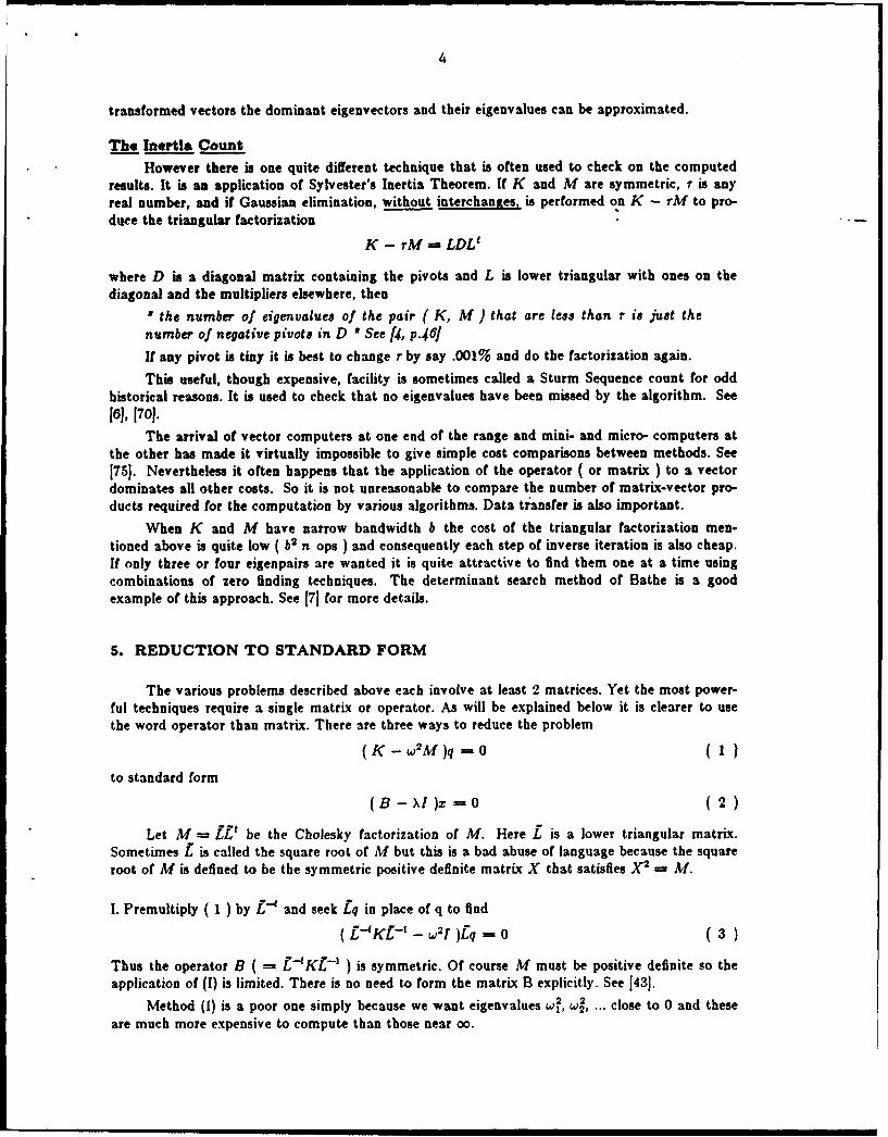
The Inertia CountHowever there is one quite different technique that is often used to check on the computed
results. It is an application of Sylvester's Inertia Theorem. If K and M are symmetric, r is anyreal number, and if Gaussian elimination, without interchanges, is performed on K - rM to pro-duce the triangular factorization
K - rM = LDLe
where D is a diagonal matrix containing the pivots and L is lower triangular with ones on thediagonal and the multipliers elsewhere, then
I the number of eigenvalues of the pair ( K, M ) that are less than r is just thenumber of negative pivots in D I See (4, P.46/
If any pivot is tiny it is best to change r by say .001% and do the factorization again.
This useful, though expensive, facility is sometimes called a Sturm Sequence count for oddhistorical reasons. It is used to check that no eigenvalues have been missed by the algorithm. See[lo, [7o.
The arrival of vector computers at one end of the range and mini- and micro- computers atthe other has made it virtually impossible to give simple cost comparisons between methods. See[75). Nevertheless it often happens that the application of the operator ( or matrix ) to a vectordominates all other costs. So it is not unreasonable to compare the number of matrix-vector pro-ducts required for the computation by various algorithms. Data transfer is also important.
When K and M have narrow bandwidth b the cost of the triangular factorization men-tioned above is quite low ( b n ops ) and consequently each step of inverse iteration is also cheap.If only three or four eigenpairs are wanted it is quite attractive to find them one at a time usingcombinations of zero finding techniques. The determinant search method of Bathe is a goodexample of this approach. See [71 for more details.
S. REDUCTION TO STANDARD FORM
The various problems described above each involve at least 2 matrices. Yet the most power-ful techniques require a single matrix or operator. As will be explained below it is clearer to usethe word operator than matrix. There are three ways to reduce the problem
(K - w2M )q = (1)
to standard form
(B- XI )z =0 (2)
Let M = i be the Cholesky factorization of M. Here E is a lower triangular matrix.Sometimes f is called the square root of M but this is a bad abuse of language because the squareroot of M is defined to be the symmetric positive definite matrix X that satisfies X2 _ M.
I. Premultiply ( 1 ) by E and seek /q in place of q to find
( f-K - 2) q f o (=3 )
Thus the operator B ( = .- K, -1 ) is symmetric. Of course M must be positive definite so theapplication of (I) is limited. There is no need to form the matrix B explicitly. See 143j.
Method (1) is a poor one simply because we want eigenvalues w, w, ...2 close to 0 and theseare much more expensive to compute than those near 0o.
5
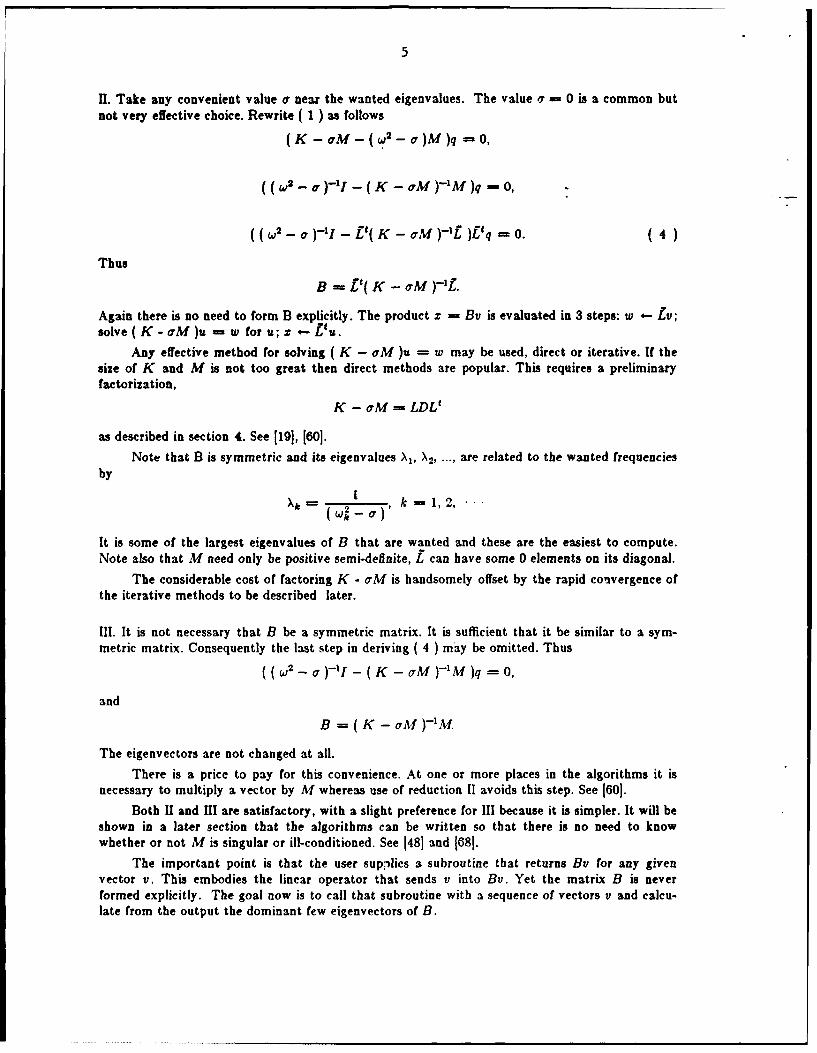
H. Take any convenient value o near the wanted eigenvalues. The value 7 = 0 is a common butnot very effective choice. Rewrite ( 1 ) as follows
(K - aM - (w' - a )M )q = 0,
((w - a )I -( K - aM )'M )q= 0,
W2( - a )-Ij ' K - aM )-0 £, f . (4)
Thus
B = ,( K - aM )-'L.
Again there is no need to form B explicitly. The product z = By is evaluated in 3 steps: w t Lv;solve (K - aM )u - w for u; z .- Vu.
Any effective method for solving ( K - aM )u - w may be used, direct or iterative. If thesize of K and M is not too great then direct methods are popular. This requires a preliminaryfactorization,
K - aM = LDLV
as described in section 4. See [191, [601.Note that B is symmetric and its eigenvalues '\, X2, ..., are related to the wanted frequencies
byI
k= (w- k =1, 2,
It is some of the largest eigenvalues of B that are wanted and these are the easiest to compute.Note also that M need only be positive semi-definite, I can have some 0 elements on its diagonal.
The considerable cost of factoring K - aM is handsomely offset by the rapid convergence ofthe iterative methods to be described later.
iii. It is not necessary that B be a symmetric matrix. It is sufficient that it be similar to a sym-
metric matrix. Consequently the last step in deriving ( 4 ) may be omitted. Thus
( (w 2 - a ) - ( K - oM )-'M )q = 0,
and
B-- K - aAf)M.
The eigenvectors are not changed at all.
There is a price to pay for this convenience. At one or more places in the algorithms it isnecessary to multiply a vector by M whereas use of reduction 1I avoids this step. See (60).
Both II and IIl are satisfactory, with a slight preference for III because it is simpler. It will beshown in a later section that the algorithms can be written so that there is no need to knowwhether or not M is singular or ill-conditioned. See 1481 and [681.
The important point is that the user supplies a subroutine that returns By for any givenvector v. This embodies the linear operator that sends v into By. Yet the matrix B is neverformed explicitly. The goal now is to call that subroutine with a sequence of vectors v and calcu-late from the output the dominant few eigenvectors of B.
6
8. SUBSPAC ITERATION ( ealled SI )
In Europe this is called the method of Simultaneous Iterations. See 1121 and 1311. For-
tunately it has the same acronym SI.Programs based on this method ar e in widespread use throughout the engineering commun-
ity for eigenvalue extraction. See 171, 18, 11, 1121, 1311. The erectivee of the pogrlms comes
(rota sophisticated implementation whose details cannot be described here. In other wrds there
is still some art ( or judgement ) required to make the implementations robust. One of thecleverest implementations is H. Rutishauser's RITZIT algorithm presented in j79] but actuallywritten in mple-196. For a brief account of it see t59, Chap.141 and J651. RITZIT had little
influence on engineers in the U.S.A. who, in the course of time, rediscovered some of
RutishauSer s devices.The basic idea is very simple. It is a block power method. The power method takes a start-
ing vector v and keeps applying the operators B to produce the so-called Krylov sequence ( or
pnvow r v nde p a
powerseque ce )v, B , B (B ), B 3, B 4,"
For almost all v the vector Bkv points in the direction of the dominant eigenvector of B as k
-0In a blck version, with block sile m, one starts with m starting vectors, the columns of a
n X m matrix V(A ).It is best to start with an orthonormal set, i.e.
( Vo}))tv(o) -
The trouble with forming BiV0°) for large k is that all its columns are dominated by the dominant
eigenvector. This defect is easily cured by orthonotmalizing the current set of m vectors from
time to time. If this is done every time B is applied then one obtains one version of Si. However
there is more thin one way to orthonormalize a set of vectors although the Gram-Schinidt process
is the most popular, In the present context there is a better wly, use the Rayleigh-Ritz approxi-
Let V be any n X m matrix whose columns are linearly independent. There is a pretty recipe
for obtaining the s set of approximate eigenvectors using just linear combinations of V's
columns. We present it with implementation Ill of section 6 in mind.
The Ra lh~t AvproxImatlons_ tr!.. Y
1. Form the m x m proiection matrices ( often called interaction matrices)
C -- VtIBV), E V(V
2. Solve the full m X m generalized eigenvalue problem ( C - OE )gi - 0, i - 1, ... , m to Bud
G = gt, "", g" ) and 0 :=a diag ( 01, ... , 0m ). Normalize the g so that gEg 1, i 1,
3. Form W - VG.
The vectors w,, ..., tom are the desired approximate eigenVectOrs. In general some of the w will be
much better approximations than others. The numbers $1, ..., 0,, are the Rayleigh-Ritz approxi-
mate eigenvalues.
The essential SI algorithm is to keep repeating these Rayleigh-Ritz approximations.
I AL oS-thm1. pick a full rank V")
7
2. for k = 1, 2, ..., until satisfied
a) obtain Rayleigh-Ritz approximations g k), 0tk)) .... (g$ ), 0 ) from Vkl)
b) compare 0?*) with st - l) to monitor convergence, j - 1, .... mc) if not satisfied set
v k) :i V(k-t)g k) for each bad j,
v k) : vk-), if 6j ha8 converged.
For a fuller discussion of SI with attention to more details of implementation see:K. J. Bathe and coworkers [7, Chap. 121; 181 for his latest.A. Jennings and coworkers [33, Chap. 10), and, in turn, [11], [121, [31), [34).
Both groups have an engineering orientation. The numerical analysts were mentioned at thebeginning of section 6.
Important ingredients to successful usage of SI are1. Choice of m
2. Choice of V(O)
3. Mechanisms for avoiding convergence to already known eigenvectors.Good variations of SI have been incorporated into a number of FEM packages.There is only one fundamental criticism to be made of SI it may use considerably more calls
to the operator subroutine than are necessary. The explanation is very simple. At every step in S[the approximations 0"-) are overwritten with better ones in yk) This overwriting discards infor-mation and the penalty can be significant. In fact it is not necessary to increase storage costs toachieve a substantial saving in computational effort.
7. THE LANCZOS APPROACH
The power of the Lanczos algorithm comes from a fortunate approximation property ofKrylov subspaces. Although it is quite surprising it is not difficult to state.
It is well known that the power sequence ( see the third paragraph of section 6 for the powersequence ), started from a random vector, converges almost always to the dominant eigendirectionof the operator B. In principle a large number of steps might be necessary. Suppose we ask adifferent question. After k-1 steps of the power method how many eigenvectors of B could beapproximated to 5 decimal accuracy by taking suitable linear combinations of our k vectors
v, By, B2 v, ..., Bk-iv ?
Remember that 5 decimal accuracy in an approximate eigenvector y means 10 decimal accuracyin the approximate eigenvalue 0 = ( ytBy )/( ytMy ).
Now for k = 1 the answer is none and for k = n, the number of degrees of freedom, theanswer is n. However these extremes are not relevant. The amazing observation is that for valuesof k between 20 and n/5 the answer is about k/2. As k increases the hit ratio improves but formost applications in Mechanics it is about 50% or better. Consequently it should be possible tocomputer 25 eigenpairs with only 50 calls on the operator ( i.e. 50 matrix-vector products ). Yetafter 50 steps the power method might well have produced only a 3 decimal approximation to asingle eigenvector.
When one recalls that the starting vector is chosen at random this phenomenon is remark-able. The eigenvalues computed in this way will be those closest to the number a that occurs in
8
the definition
B (K - M'M.
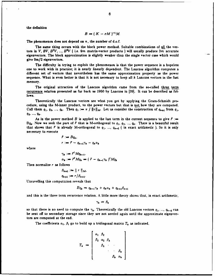
The phenomenon does not depend on n, the number of d.o.f.The same thing occurs with the block power method. Suitable combinations of all the vec-
tors in V, BV, B V, ..., B V ( i.e. 0m matrix-vector products ) will usually produce 3m accurateeigenvectors. The block approximation is slightly weaker than the single vectoi case which wouldgive 9m/2 eigenvectors.
The difficulty in trying to exploit the phenomenon is that the power sequence is a hopelessone to work with in practice; it is nearly linearly dependent. The Lanczos algorithm computes adifferent set of vectors that nevertheless has the same approximation property as the powersequence. What is even better is that it is not necessary to keep all k Lanczos vectors in the fastmemory.
The original attraction of the Lanczos algorithm came from the so-called three termrecurrence relation presented as far back as 1950 by Lanczos in [301. It can be described as fol-lows.
Theoretically the Lanczos vectors are what you get by applying the Gram-Schmidt pro-cedure, using the M-inner product, to the power vectors but that is not how they are computed.Call them q1, q2, ..., q,. Then q, := v / IIvIIM. Let us consider the construction of q,+ from q1,q2, -- qb.
As in the power method B is applied to the last term in the current sequence to give F :=Bqt. Now we seek the part of F that is M-orthogonal to qj, q2, ..., qk. There is a beautiful resultthat shows that F is already M-orthogonal to q1 , ..., q,-2 ( in exact arithmetic ). So it is onlynecessary to execute
F := Bqk,
r qk-:O k - qk0 k
where
ak :- F = Mq (- ,atk :- F'Mqj, F ( - qk--t )'Mqk
Then normalize r as follows
qk+l := r/ k+l.
Unravelling this computation reveals that
Bq, ' qk-1rk + qak + qk+1ik+l
and this is the three term recurrence relation. A little more theory shows that, in exact arithmetic,
=f k 2
so that there is no need to compute the Yk. Theoretically the old Lanczos vectors q1 ... , qk-2 canbe sent off to secondary storage since they are not needed again until the approximate eigenvec-
tors are computed at the end.
The coefficients aj, 0( go to build up a tridiagonal matrix Tk as indicated,
of 1 02
2 C12 03
.k Ok
,,~~~O akia I
9
This matrix holds all the essential information. Notice how little work there is in computing qk+lcompared with one step of subspace iteration (SI).
Suppose k is the last step. To complete the calculation we proceed as follows,
1) Compute all eigenvalues and eigenvectors of Tk, TkaI = -- O, i-1, ..., k wherek
= fj) 1.
2) Select those pairs ( 0j, 8j ) with the property I s,(k) I < 10 " .
3) For the values of i found in 2) recall the Lanrzos vectors and compute
=j q 1 (1) + q2 8j(2) + - + qak).Y
The pairs ( 6j, y( ) are approximate eigenvectors with the property
11 Byj - y IIM = 10'0k+l.
The 9j will be accurate to about 10 significant figures. More precisely there is an eigenvalue X ofB such that
I - 0€1 __ lO- 01/ gap
where gap = min I p - I - min I 8j+1 - I, I Oi - Oij I ) and j is the closest eigen-value of B to 8j except for X. See 1561.
The description given above ignored the important issue of detecting k, the right step atwhich to stop. See [261, [561 and [691.
Orthogonality Loss
The preceding section may seem too good to be true. And it is. Finite precision arithmeticprevents the Lanczos vectors from being M-orthogonal or even close to it. In Fig.1 we show thatmatrix QtMQk, where Qk = ( qj, ..., qk ). It should be the identity matrix.
This defect gave the Lanczos algorithm a bad reputation and only a few engineers per-severed with it during the 1960s. See [771 & [78]. In 1971 C. C. Paige, in a remarkable thesis, wasthe first to explain this orthogonality loss in a satisfactory way. Once this understanding spread itwas not difficult to find ways to handle the problem. In particular he showed that the originalalgorithm is not unstable; you can extract all eigenvaiues.
It is beyond the scope of this brief paper to expound Paige's contribution. For a text bookaccount for numerical analysts see 1 59, Chap.13 ] and for a more detailed, but lucid, presentationsee two papers by Paige, [51] and [52].
What we can say is that there are three different ways of responding to orthogonality losswhen executing the three term recurrence. The first, advocated by Paige himself ( though not inthe context of Mechanics ), has been fully developed by Cullum and Willoughby, see [13], [14], andalso Parlett k Reid [55]. The idea is to keep the original algorithm. The result is that the methodbecomes truly iterative, it does noL stop at step n. Nevertheless it is possible to deduce the trueeigenvalues of B from the computed tridiagonal T. However the number of steps required growsby a factor of 2 or 3 at least. Moreover eigenvectors must be computed separately. These pro-grams seem best suited for computing all the eigenvalues of B. Engineering development alongthese lines are 1181 and [771.
The opposite extreme explicitly applies the Gram-Schmidt process to make Bq1 orthogonalto qj, q, ..., q-2 at each step. Besides the cost of this extended computation there is the need toaccess all Lanczos vectors at each step. However the minimal number of steps will be taken. Forshort Lanczos runs of about 20 steps the cost of this approach is not heavy. See [10], [19], [20],[211, (281, [491, 1501, and [751.
- --- -- --- --- --- - ----- - - - - - O N N N~ Y Y V
r ~ll m m T v T Aq
-- 0~dn -NOO UNNNNV7 ~ ~ YtYatgvV
11
A third approach is based on the observation that it suffices to maintain semi-orthogonalityto enjoy the main advantages of full-orthogonality. If tVie unit roundoff in the arithmetic unit is ethen two vectors of norm one are semi-orthogonal if their inner product does not exceed V1 inmagnitude. Moreover semi-orthogonality among the Lanczos vectors can be maintained for about1/3 the cost of maintaining c-orthogonality. In particular the minimal number of Lanczos stepswill be taken. See (58J, [691 and [711.
It seems likely that in Mechanics it will be preferable to keep the number of calls on theoperator B to a minimum. For applications in which the whole spectrum is wanted the firstapproach is the most attractive.
To complicate the issue there is the extra possibility of using block versions of the Lanczosalgorithm. That leads to the next section.
Block Lanczos
Just as the power method is readily extended to a block form ( namely subspace iterationso is the Lanczos recurrence extended to work with several vectors simultaneously. A block size Iis chosen and a sequence of n X1 Lanczos matrices Q 1, Q 2, ... , Qk is constructed to satisfy
1. Q5MQJ = It
2. BQj = Q= -,B' + QjAj + Qj+1 B+.
Here Bi is an I X I upper triangular matrix and Aj is I X I symmetric. The associated matrix Tk isno longer tridiagonal but has semi-bandwidth I. Consequently all calculations involving T aremore costly than with simple Lanczos.
The original motivation for block versions of Lanczos was to allow the detection of multipleeigenvalues of B. In exact arithmetic the simple Lanczos algorithm cannot distinguish multiplici-ties but, in practice, roundoff error ensures that the right number of copies of an eigenvalue willbe found, but at the cost of a few extra Lanczos steps, provided that the Lanczos vectors are keptorthogonal or semi-orthogonal. See [601.
Theoretically the simple Lanczos algorithm has the best approximation properties for agiven number of calls on the operator B.
However the increasing complexity of modern operating systems and storage managementhas provided a powerful incentive to use block codes despite their increased cost per step. If thetriangular factor L in LDLt = K - tiM cannot be stored in the fast memory then considerabletransfer between primary and secondary storage is needed to invoke the operator B. In such casesit is advantageous to let B operate on several vectors at once. The precise number is problem andcomputer system dependent.
We can say that in each case there is a maximal number I such that the cost of applying Bto I vectors is within 10% of the cost of applying B to one vector. In a good number of cases I =1 but, in general 1, as defined, is the correct block size - assuming that I n-vectors can be held inprimary storage along with sections of L.
The block Lanczos program embedded in MSC/NASTRAN Version 65 permits the user tospecify the block size. See [261,1391. Block Lanczos methods are described in [251, [261, [281, [451,(631, 1871 & 1691.
S. LANCZOS VERSUS SUBSPACE ITERATION (SI)
A comparison between two implementations is presented in 1461 although the experimentswere made in 1980. Our only interest here is to illustrate the approximation power that comesfrom using combinations of the power vectors instead of using just the most recent one.
12
A three dimensional building frame was analyzed by the finite element method. There were468 d.o.f. and the 60 dominant mode shapes were to be computed. This is more than 10% of thespectrum. The interesting question is how many calls on the operator subroutine [ i.e. solve (K - aM )r = Mq for r I are needed for the computation of these 60 eigenvectors.
Recall that SI has to choose the subspace size. A well-known rule selects 68 but for the givenapplication this is inefficient. We show below in Table I the number of operator calls required byseveral programs.
Several points need to be made in order to see the significance of Table 1.i) The program SI (accelerated) incorporates a lot of clever tricks for improving the perfor-
mance of SI. See 181 for the details. Consequently it is more instructive to consider a straightforward implementation, namely SI (basic), to appreciate the theoretical improvement thatcomes from using a Krylov subspace. Figures are not available for SI (basic) used withq = 20 but we may infer that at least 2000 calls on the operator subroutine would be made.Yet the bottom line of Table 1 shows that only 120 are needed by a rival method startingfrom a random vector.
ii) SI (accelerated) used 12 different shifts ( i.e. factorizations of K - GAf ) to achieve itsimprovements whereas LANSO used only one. However LANSO could also benefit from useof more than one shift as is shown in (201. The benefit is in storage requirements, not callson the operator. For example, one could use 4 shifts in turn making about 31 or 32 calls onthe operator each time while picking up 15 eigenvectors. In this way there only needs to bestorage for 35 vectors. That means that larger problems could be solved completely insidethe fast memory. The selection of shifts is an interesting topic. See [19 and [35).
iii) There is a price to be paid for achieving this very small number of calls on the operator sub-routine. It is necessary to keep all the Lanczos vectors somewhere because they are recalledat the end to accumulate the eigenvectors. It turns out that they are needed more oftenthan that because of roundoff error. In the simplest implementations the new Lanczos vectoris explicitly orthogonalized against all previous Lanczos vectors at each step. This is overkill.Nevertheless it is necessary to do the orthogonalization from time to time about ( one stepin four, on the average ) in order to keep the number of steps to a minimum.
More information on these topics is contained in [191, [211, 1481.iv) It would be more informative to compare SI with a block Lanczos code but we are not aware
of such a trial.
9. SINGULAR M
The null space of At is also the nullspace of B - ( K - cfA )'At ( i.e. Afv - 0 if, andonly if, By = 0 ). Every nontrivial vector in this subspace .N(B) may be considered an eigenvec-tor of B with eigenvalue oo. Complementary to N(B) is R(B), the range space of R. It is spannedby the eigenvectors belonging to the finite eigenvalues.
13
By restricting attention to R(B) the regular case is recovered. Of course R(B) is not knownbut in exact arithmetic it is easy for all computed vectors to be kept in R(B). It suffices that thestarting vectors, for SI and Lanczos, be in R(B). Unfortunately rounding errors introduce into allcomputed vectors components in N(B). With Lanczos these components grow steadily as thecomputation proceeds but this feature is not at all evident because the M-inner product is blind tosuch errors. Engineers are often tempted to stay in R(B) by using static condensation, see [321,but this usually spoils the sparsity structure of the reduced matrices.
There is an easy cure. Each approximate eigenvector y may be projected back onto R(B) byforming By and then normalizing. However this is expensive. If m approximate eigenvectors arecomputed using only 2m calls on B then a further m calls on B to purify the eigenvectors addsapproximately 50% to the cost.
Is there a way to purify y without making any more calls on B ?
With the Lanczos algorithm there is a nice trick. See [481. It is easy to explain and imple-ment.
Let ( $I, yi ) be an approximate eigenpair with
=i-- QMe =' ±'qk6(k).k=1[
See section 7 for notation. The next, so-far-unused Lanczos vector qJ+1 is available. It turns outthat
By - yi1 + qj+1,8j+jai(i)
to within roundoff terms. Consequently it is only necessary to replace Y1 by
ff, := y + qi+,( fli.1si(j)/oi ).
The quantity iy+i(j) will already.be known since it provides an error bound on yi. There is noneed to have 8,(j)2 < unit roundoff ( from section 7 ) so the correction to yi is far from negligi-ble. See the Table in (481 for the striking effect.
This modification makes a small improvement even when M is invertible. Consequently itshould be made automatically and there is no need for the program to know whether or not M issingular. A beautiful result.
10. LOOKING AHEAD
The linear eigenvalue problem K - XM, with real eigenvalues, is in good shape but thereare many challenges ahead.
1. Efficient, robust techniques for quadratic eigenvalue problems ( as indicated in Section 3 ).Standard practice encourages reduction to a linear problem, see [23] and [36] for example,but this may not be optimal. See [661 and 1741.
2. Problems with complex conjugate pairs of eigenvalues ( as indicated in Section 3 ). Thematrices described in this paper can be extended to the nonsymmetric case. See 130], 172] forSI and [241, [54] for Lanczos. Also see [64].
3. Exploiting vector computers to the full.
4. The effect of parallel computers.
That can wait for the next issue of State-of-the-Art!
14
REFERENCES
1. "Matrix Eigensystem Routines - EISPACK Guide (1976)," in Lecture Notes in Computer Science,Second Edition, ed. C. B. Moler, vol. 6, Springer, New York.
2. "Matrix Eigensystem Routines - EISPACK Guide Extension (1977)," in Lqcture Notes in Computer
Science, Second Edition, ed. C. B. Moler, vol. 51, Springer, New York.
3. NASTRAN Users Manual (1977), NASA Langley Research Center, Hampton, Virginia.
4. HARWELL Subroutine Library (1981), Computer Science and System Division, Atomic EnergyResearch Establishment, Harwell, Oxfordshire, England.
5. Awsleend, L. and P. Bjorstad (1983), "The generalized eigenvalue problem in ship design andoffshore industry," in Matrix Pencils, ed. A. Ruhe.
6. Barth, W., R. S. Martin, and J. H. Wilkinson (1967), "Calculation of the eigenvalues of a symmetrictridiagonal matrix by the method of bisection," Numer. Math., vol. 9, pp. 386-393.
7. Bathe, K.-J. and E. L. Wilson (1976), Numerical Methods in Finite Element Analysis, Prentice, En-glewood Cliffs, New Jersey.
8. Bathe, K.-J. and S. Ramaswamy (1980), "An accelerated subspace iteration method," Comput.Methods Appl. Mech. Engrg., vol. 23, pp. 313-331.
9. Butscher, W. and W. E. Kammer (1976), "Modification of Davidson's method for the calculation ofeigenvalues and eigenvectors of large real symmetric matrices: " Root- homing procedure","J.Comput. Phys., vol. 20, pp. 313-325.
10. Carnoy, E. and M. Geradin (1982), "On the practical use of the Lanczos algorithm in finite elementapplications to vibration and bifurcation problems," in Proceedings of the Conference on MatrixPencils, Held at Lulea, Sweden, March 198, University of Umea, ed. Axel Ruhe, pp. 156-176,Springer Verlag, New York.
11. Clint, M. and A. Jennings (1970), "The evaluation of eigenvalues and eigenvectors of real symmetricmatrices by simultaneous iterations," Compt. J., vol. 13, pp. 76-80.
12. Corr, R. B. and A. Jennings (1976), "A simultaneous iteration algorithm for symmetric eigenvaluesproblems," Internat. . Numer. Methods Engrg., vol. 10, pp. 647-663.
13. Cullum, J. and R. A. Willoughby (1979), "Lanczos and the computation in specified intervals of thespectrum of large sparse real symmetric matrices," in Sparse Matrices and their uses, ed. Duff, pp.220-255, Acad. Press.
14. Cullum, J. and R. A. Willoughby (1984), "Lanczos Algorithms for Large Symmetric Matrices,"Uaers Guide, vol. 1 and 2, Birkhauser, Boston.
15. Cuppen, J. M. M. (1981), "A Divide and Conquer Method for the Symmetric Tridiagonal Eigenprob-lem," Num. Math., vol. 36, pp. 177-195.
16. Daniel, W. J. T. (1980), "Modal Methods in Finite Element Fluid - Structure Eigenvalue Problems,"Int. J. Num. Meth. Eng., vol. 15, no. 8.
17. Dongarra, J. and D. Sorenson (1987), "A Fully Parallel Algorithm for the Symmetric EigenvalueProblem," SISSC. To appear
18. Edwards, J. T., D. C. Licciardello, and D. J. Thouless (1979), "Use of the lanczos method for findingcomplete sets of eigenvalues of large sparse symmetric matrices," J. Inst. Math. Appl., pp. 277-283.
15
19. Ericsson, T. and A. Ruhe (1980), "The spectral transformation Lanczos method for the numericalsolution of large sparse generalized symmetric problems," Math. Comp., vol. 35, pp. 1251-1268.
20. Ericsson, T. and A. Ruhe (1082), "STLM - a software package for the spectral transformation Lanc-zos algorithm," UMINF-101.82, U. Umea.
21. Ericsson, T. (1983b), "Algorithm for large sparse symmetric generalized eigenvalue problem,"UMINF-108.83, U. Umea.
22. Felippa, C. A. (1977), "Procedures for Computer Analysis of large nonlinear structural systems,"Proceedings of the International Symposium on Large Engineering Systems held at the Univ. of Man-itoba, Winnipeg, Canada in August 1976., Pergamon Press.
23. Fricker, A. J. (1983), "A Method for Solving High - Order Real Symmetric Eigenvalue Problems,"
Int. 1. Num. Meth. Eng., vol. 19, no. 8.
24. Gerardin, M. (1977), "Application of the Biorthogonal Lanczos Algorithm," LTAS.
25. Golub, G. H. and R. Underwood (1977), "The block Lanczos method for computing eigenvalues," inMathematics Software III, ed. J. R. Rice, pp. 361-377, Academic Press, New York.
26. Grimes, R., J. G. Lewis, and H. Simon (1986), "The Implementation of a block, shifted and invert-ed, Lanczos algorithm for eigenvalue problems in structural engineering," Tech. Report ETA-TR-39,Boeing Computer Services, Seattle, WA..
27. Gupta, K. K. (1974), "Eigenproblem solution of damped structural systems," Int. J. Num. Meth.Eng., vol. 8, pp. 877-911.
28. Gupta, K. K. (1978b), "Development of a finite dynamic element for three vibration analysis oftwo-dimensional structures," Internat. . Numer. Methods Eng., vol. 12, pp. 1311-1327.
29. Iyer, M. S. (1981), "Eigensolution using Langrangian Interpolation," Int. J. Num. Met. Eng., vol.17, no. 10.
30. Jennings, A. and W. J. Stewart (1975), "Simultaneous iteration for partial eigensolution of real ma-trices," J. Inst. Math8. Applics., vol. 15, pp. 351-361.
31. Jennings, A. and T. J. A. Agar (1981), "Progressive Simultaneous Inverse Iteration for SymmetricLinearized Eigenvalue Problems," Computers and Structures, vol. 14, no. 1-2.
32. Jennings, A. (1973), "Mass condensation and simultaneous iteration for vibration problems," Int. J.for Num. Methods in Engng.,, vol. 6, pp. 543-562.
33. Jennings, A. (1977), in Matrix Computation for Engineers and Scientists, Wiley, New York.
34. Jennings, A. (1981), "Eigenvalue methods and the analysis of structural vibration," in Sparse Ma-trices and their Uses, ed. Duff, pp. 109-138.
35. Jensen, P. S. (1972), "The solution of large eigenproblems by sectioning," SIAM J. Numer. Anal.,vol. 9, pp. 534-545.
36. Johnson, C. P. etc (1980), "Quadratic Reduction for the Eigenproblem," Int. J. Num. Meth. Eng.,vol. 15, no. 6.
37. Kats, J. M. van and H. A. van der Vorst (1977), "Automatic monitoring of Lanczos schemes forsymmetric or skew symmetric generalized eigenvalue problems," Acad. Comp. Centrum ReportTR-7, U. Utrecht.
38. Komzsik, L. and G. A. Dilley (1985), Practical Experiences with the Lanczos Method. private com-munication concerning MSC/NASTRAN Version 65
39. Lanczos, C. (1950), "An iteration method for the solution of the eigenvalue problem of lineardifferential and integral operators," J. Res. Nat. Bur. Stand., vol. 45, pp. 255-282.
16
40. Levit, Itzhak (1984), "A New Numerical Procedure for Symmetric Eigenvalue Problems," Comput-ers and Structures, vol. 18, no. 6.
41. Lewis, J. G. and R. G. Grimes (1981), "Practical Lanczos algorithms for solving structural engineer-
ing problems," in Sparse Matrices and their Uses, ed. Duff, pp. 349-355, Acad. Press.
42. Lob, C. H. (1984), "Chebyshev Filtering and Lanczos' Process in the Subspace Iterative Method,"Int. J. Num. Meth. Eng., vol. 20, no. 1.
43. Martin, R. S. and J. H. Wilkinson (1968), "Reduction of the symmetric eigenproblem Ax---Bx andrelated problems to standard form," Numer. Math., vol. 11, pp. 99-110.
44. Matthies, H. and G. Strang (1979), "The Solution of Nonlinear Finite Element Equations," Int. J.Num. Meth. Eng., vol. 14, pp. 1613-1626.
45. Matthies, H. G. (1985), "A Subspace Lanczos Method for the Generalized Symmetric Eigenprob-lem," Computers and Structures, vol. 21, pp. 319-325.
46. Nour-Omid, B., B. N. Parlett, and R. L. Taylor (1983), "Lanczos versus subspace iteration for solu-tion of eigenvalue problems," Internat. J. Numer. Methods Engrg., vol. 19, pp. 859-871.
47. Nour-Omid, B.. B. N. Parlett, and R. Taylor (1983), "Lanczos versus Subspace Iteration for Solu-tion of Eigenvalue Problems," Int. J. Num. Meth. Eng., vol. 19, no. 6.
48. Nour-Omid, B., B. N. Parlett, T. Ericsson, and P. S. Jensen (1987), "How to implement the SpectralTransformation," Math. Comp., vol. 48.
49. Ojalvo, I. U. and M. Newman (1970), "Vibration modes of large structures by an automatic matrix-reduction method," AJAA Journal, vol. 8, pp. 1234-1239.
50. Ojalvo, I. U. (1985), "Proper Use of Lanczos Vectors for Large Eigenvalue Problems," Computersand Structures, vol. 20, no. 1-3.
51. Paige, C. C. (1976), "Error analysis of the Lanczos algorithms for tridiagonalizing a symmetric ma-tri'x," J. Inst. Math. Appl., vol. 18, pp. 341-349.
52. Paige, C. C. (1980), "Accuracy and effectiveness of the Lanczos algorithm for the symmetric eigen-problem," Linear Algebra Appl., vol. 3-1, pp. 235-258.
53. Papadrakasis, M. (1984), "Solution of the Partial Eigenproblem by Iterative Method," Int. J. Num.Meth. Eng., vol. '-.0, no. 12.
54. Parlett, B. N., D. R. Taylor, and Z. A. Liu (1985), "A Look-Ahead Lanczos Algorithm for Unsym-metric Matrices," Math. Comp., vol. 44, pp. 105-124.
55. Parlett, B. N. and D. S. Scott (1979), "The Lanczos algorithm with selective reorthogonalization,"Math. Cornp., vol. 33, pp. 217-238.
56. Parlett, B. N. and J. K. Reid (1981), "Tracking the progress of the Lanezos algorithm for large sym-metric matrices," IAfA J. Numer. Anal., vol. 1, pp. 135-155.
57. Parlett, B. N. and B. Nour-Omid (1985), "The Use of Refined Error Bounds when Updating Eigen-values of Tridiagonals," J. Lin. Ag. O Appls., vol. 68, pp. 179-220.
58. Parlett, B. N., B. Nour-Omid, and J. Natvig, "Implementation of Lanczos algorithms on VectorComputers," Supercomputer Applications, Plenum Press, New York, 1985.
59. Parlett, B. N. (1980), in The Symmetric Eigenvalue Problem, Prentice-Hall, Englewood Cliffs, NJ.
60. Parlett, B. N. (1980b), "How to solve (K-AM)z = 0 for large K and M.." Numer. Methods Engrg.,Dunod, Paris.
17
61. Parlett, B. N. (1084), "The Software Scene in the Extraction of Eigenvalues from Sparse Matrices,"SIAM J. Sci. Slat. Comput., vol. 5, pp. 590-603.
62. Robati, P. (1984), "The Accelerated Power Method," Int. 1. Num. Meth. Eng., vol. 20, no. 7.
63. Ruhe, A. (1979), "Implementation aspects of band Lanczos algorithms for computation of eigen-values of large sparse symmetric matrices," Math. Comp., vol. 33, pp. 680-687.
64. Saad, Y. (1981), "Krylov Subspace methods for solving large unsymmetric linear systems," Math.Comp., vol. 37, pp. 105-126. -
65. Schwarz, H. R. (1977), "Two algorithms for treating Ax=-kBx ," Compul. Methods Appl. Mech.Engrg., vol. 12, pp. 181-109.
66. Scott, D. S. and R. C. Ward (1982), "Solving symmetric-indefinite quadratic lambda-matrix prob-lems without factorization," SIAM J. Sci. Statist. Comput., vol. 3, pp. 58-67.
67. Scott, D. S. (1979), "Block Lanczos software for symmetric eigenvalue problems," ORNL ReportCSD-48, Oak Ridge, Tennessee.
68. Scott, D. S. (1980), "The advantages of inverted operators in Rayleigh-Ritz approximations," SIAMJ. Sci. Statist. Comput., vol. 3, pp. 68-75.
60. Scott, D. S. (1981), "The Lanczos algorithm," in Sparse Matrices and Their Uses, ed. I. S. Duff, pp.139-150, Academic Press, New York.
70. Scott, D. S. (1981b), "Solving sparse symmetric generalized eigenvalue problem without factoriza-tion," SIAM J. Numer. Anal., vol. 18, pp. 102-110.
71. Simon, H. D. (1984), "The Lanczos algorithm with partial reorthogonalization," Math. Comp., vol.42, pp. 115-142.
72. Stewart, W. J. and A. Jennings (1981), "A simultaneous iteration algorithm for real matrices," ACMTOMS, vol. 7, pp. 184-198.
73. Utku, Senol etc (1984), "Computation of Eigenpairs of Ax=---x for Vibration of Spinning Deform-able Bodies," Computers and Structures, vol. 19, no. 5/6.
74. Veselic, K. (1980), "On Optimal Linearizations of a Quadratic Eigenvalue Problem," Linear & Mul-tilinear Algebra, vol. 8, pp. 253-258.
75. Weingarter, V. I. etc (1983), "Lanczos Eigenvalue Algorithm for Large Structures on a minicomput-er," Computers and Structures, vol. 16, no. 1-4.
76. Wellford, L. Carter etc (1980), "Post-buckling Behaviour of Structures using a Finite Element -Nonlinear Eigenvalue Technique," Int. J. Num. Meth. Eng., vol. 15, no. 7.
77. Whitehead, R. R., A. Watt, B. J. Cole, and I. Morrison (1977), "Computational methods for nuclearshell-model calculations," Advances in Nuclear Physics, vol. 9, pp. 123-176, Plenum Press, NewYork.
78. Whitehead, R. R. (1972), "A numerical approach to nuclear shell-model calculations," Nuct. Phys.,vol. A182, pp. 290-300.
79. Wilkinson, J. H. and C. Reinsch (1971), Handbook for Automatic Computation: vol.!!, Linear Algebra
, Springer-Verlag, New York.
80. Wilkinson, J. H. (1066), The Algebraic Eigenvalue Problem, Oxford Univ. Press.
81. Wilson, E. L., M. W. Yuan, and J. M. Dickens (1982), "Dynamic analysis by direct superposition ofRitz vectors," E.E.Str. Dyn., vol. 10, pp. 813-821.
82. Yang, W. H. (1983), "A method for Eigenvalues of Sparse ).. matrices," Int. J. Num. Meth. Eng.,vol. 19, no. 6.