Received 16 July 2005, in final form 4 May 2006Published 15 January 2007Online at stacks.iop.org/SMS/16/S51
AbstractThis paper presents a constitutive model for shape-memory alloys that buildson ideas generated from recent micromechanical studies of the underlyingmicrostructure. The presentation here is in one dimension. It is applicable ina wide temperature range that covers both the shape-memory effect andsuperelasticity, is valid for a wide range of strain rates and incorporatesplasticity. The thermodynamic setting of the model is explained and themodel is demonstrated through examples.
1. Introduction
Shape-memory alloys are widely used for a variety ofapplications including micro-actuators, cell phone antennas,energy absorption and biomedical devices. These materialsexhibit a strongly nonlinear thermo-mechanical behaviorassociated with abrupt changes in their lattice structurecalled martensitic phase transformation. Two commonmanifestations of this phase transformation are the shape-memory effect, wherein an apparently plastic deformationsustained below some critical temperature is recovered onheating above it, and superelasticity, wherein significantdeformations suffered under loading are recovered onunloading.
The applications of these materials and the need fora design tool have motivated a number of macroscopicconstitutive models for these materials (see for exam-ple [28, 24, 18, 36, 14, 37, 30, 19, 12, 3, 4] and the referencestherein). While some of them have been adapted from otherphenomena like plasticity, a number of them have tried to buildin true micromechanical features. Amongst the latter, there is awhole range that balance simplicity against detail. For a modelto be usable in the context of design, it has to be relatively sim-ple, and it should be capable of being implemented in standardstress-analysis software. At the same time, it has to incorpo-rate realistic physics. Indeed, each object and function in themodel should in principle be computable from a lower-scale
1 Author to whom any correspondence should be addressed.
model, but possible to fit to empirical data. This would en-sure that the model is widely applicable: it has to be applicablein a wide range of temperatures so that it captures both theshape-memory effect and superelasticity; it has to be adaptableto a wide range of materials and textures; it has to hold for awide range of loading rates. Finally, since phase transforma-tion often competes with plasticity in shape-memory alloys, themodel should incorporate this phenomenon as well.
The last couple of decades has also brought about anincreasingly sophisticated understanding of the microstruc-ture of shape-memory alloys and its relation to macroscopicproperties in both single and polycrystals (see for exam-ple [27, 8, 5, 9, 26, 35, 21, 22, 34, 13, 17, 20, 33, 2] and the ref-erences therein). In this paper, we present a constitutive modelthat builds on the concepts that have emerged from this analy-sis of microstructure.
The shape-memory effect and superelasticity are conse-quences of a martensitic phase transformation, which is a dif-fusionless first-order phase transformation between a high-temperature austenite phase and a low-temperature marten-site phase. The crystallographic symmetry of the austenite ishigher than that of the martensite, and consequently one canhave a number of symmetry-related variants of martensite. Thedifferent variants of martensite, along with the austenite, formcomplex microstructures that can evolve with load and temper-ature. A key difficulty in the constitutive modeling of thesematerials is to find an effective means of describing this evolu-tion, especially in polycrystals.
We address this issue in our model by introducing theidea of the effective transformation strain. It is the average
transformation strain of the different variants averaged overa representative volume containing multiple grains after thematerial has formed an allowable microstructure. It is allowedto take any value in the set of effective transformation strains,or set of effective recoverable strains. The micromechanicalbasis for this set can be found in Bhattacharya and Kohn [9](also see [11]). It is also the convex dual of the transformationyield set introduced by Lexcellent and his coworkers [20]. Thisset depends on the material and the texture of the specimen, andcan be easily fitted to experiment. In one dimension, it is theinterval from the recoverable compressive to the recoverabletensile strain. A second important idea in this paper is the useof kinetic relations that cover a wide range of strain rates.
This paper develops the model in one dimension. Wehave generalized it to three dimensions elsewhere [31]. Wehave also adapted this model for the study of martensitic phasetransformations in iron under dynamic loading [32]. Section 2introduces the model and describes its thermodynamic setting.Section 3 demonstrates the model by studying its responseto applied stress under a variety of conditions. Since load-controlled experiments are difficult, especially at high rates, themodel is also studied for its response to Kolsky bar experimentsin section 4. We conclude in section 5 with a brief discussion.
2. A thermo-mechanical model
In this section we develop and discuss our phenomenologicalconstitutive model within a continuum thermodynamicframework.
2.1. Kinematics
We are interested in a model that can be used at themacroscopic scale for the design of devices and structures. Sowe take a multiscale point of view and think of each materialpoint of our continuum as corresponding to a representativevolume element (RVE) consisting of a number of grains, eachcontaining a complex microstructure of austenite and variantsof martensite. We introduce two kinematic or field or internalvariables to represent the consequence of microstructure inan RVE: the volume fraction of martensite, λ(x, t), and theeffective transformation strain of the martensite, εm(x, t).
λ(x, t) denotes the net or average volume fraction of themartensite; i.e., this would be the value we would obtainif we were to visit each grain in the RVE correspondingto the material point x at time t , add up the volume ofall variants of martensite (self-accommodating, internallytwinned, detwinned etc) and divide by the total volume of theRVE. To be precise, let χ i j denote the characteristic functionof the j th correspondence variant of martensite in the i th grainof the RVE. This function is equal to one at all positionsoccupied by the j th variant in the i grain and is equal to zerootherwise. Then χ i = ∑N
j=1 χ i j is the characteristic functionof martensite in the i th grain where N , the number of variants,is given by the crystallography of the transformation. Wedefine the volume fraction as
λ = ⟨χ i
⟩ =⟨
N∑
j=1
χ i j
⟩
(1)
where 〈·〉 denotes the mean or expected value over all grainsin the RVE, i.e. over all i . λ is constrained to lie betweenzero and one, with zero signifying that the entire RVE is inthe austenite phase and one signifying that the entire elementis in the martensite phase.
Since λ cannot differentiate between the different mi-crostructures of martensite like self-accommodating, internallytwinned, detwinned etc, we introduce the second internal vari-able εm(x, t). This is the strain we would obtain if we were tovisit every grain in the RVE corresponding to the material pointx at time t and average over the transformation or stress-freestrain of all the variants of martensite. To be precise, let ε
i jm de-
note the transformation or stress-free strain of the j th variantof martensite in the i th grain in the RVE. It is given by
εi jm = RT
i ε jm Ri (2)
where εjm is the transformation strain of the j th correspondence
variant in a reference crystal and is given by crystallography ofthe transformation, while Ri is the rotation matrix that givesthe orientation of the i th grain and is given by the texture ofthe material. We define the effective transformation strain as
εm =⟨
N∑
j=1
χ i jεi jm
⟩
. (3)
As the material forms different microstructures, thearrangement of variants and thus χ i j changes, and εm(x, t)takes different values. We are only interested in compatiblemicrostructures, and thus we cannot form any arbitrary mixtureof variants. Consequently, εm cannot take any arbitraryaverage value, but is restricted to those that are obtained fromcompatible arrangements. We denote the set of all possiblevalues of εm as the set of effective transformation strains orthe set of effective recoverable strains, P . This set P dependson the crystallography of the material and the texture of thespecimen. In a single crystal, P is the set of all possibleaverage transformation strains associated with compatiblemicrostructures of the different variants of martensite. In apolycrystal, the set P is the the macroscopic averages of locallyvarying strain fields which can be accommodated within eachgrain by a compatible arrangement of the martensite variants.One can calculate this set in various examples of interest andestimate them in others [9, 8, 11]. Alternately, one can useexperimental measurements of recoverable strain to fit this set.
Note that we do not track the individual volumefractions of the different volumes of martensite. This is toodifficult, especially in a polycrystal, where the different grainsbehave differently depending on orientation, inter-granularconstraints and long-range cooperative effects. However, weimplicitly account for these effects by tracking the effectivetransformation strain and confining it to the set P , whichdepends on material and texture. In other words, the set Pincorporates information about the material crystallography,specimen texture and also intergranular constraints.
The set P can be quite complicated in multipledimensions, but it is relatively simple in one dimension. It is aninterval [εc
m, εtm] where εc
m < 0 denotes the largest recoverablecompressive strain and εt
m > 0 denotes the largest recoverabletensile strain.
S52
A micromechanics inspired constitutive model for shape-memory alloys: the one-dimensional case
In summary, the consequences of the microstructure at amaterial point are specified by two internal variables λ and εm
which are subject to the following constraints.
λ ∈ [0, 1] and εm ∈ P = [εcm, εt
m]. (4)
Finally, we introduce the plastic strain εp as an additionalfield variable. Putting everything together, we say that the totalstrain can be divided into three parts, elastic, transformationand plastic:
ε(x, t) = ∂u
∂x= εe(x, t) + λ(x, t)εm(x, t) + εp(x, t). (5)
It is worth noting that the effective transformation strain ofthe RVE is λεm since λ is the volume fraction of martensite,εm is the effective transformation strain of the martensite andthe transformation strain of the austenite is zero by choice ofreference configuration.
2.2. Balance laws
We assume that the usual balance laws hold. The first is thebalance of linear momentum
ρutt = σx (6)
where ρ is the (referential) mass density and σ is the (Piola–Kirchhoff) stress.
Second, we assume the balance of energy. Writing thebalance of energy for any part of the body, localizing andusing (6), we obtain
ε = −qx + r + σ ε. (7)
Above, ε denotes the internal energy density, q the heat fluxand r the radiative heating.
Finally, we write the second law of thermodynamics or theClausius–Duhem inequality, again in local form:
η �(−q
θ
)
x+ r
θ⇒ θη � −qx + qθx
θ+ r. (8)
Here, η is the entropy density and θ the (absolute) temperature.Using (7) in the second law (8), we obtain
−ε + θη + σ ε − qθx
θ� 0. (9)
It is now convenient to introduce Helmholtz free energy densityW = ε − θη and rewrite the second law in the following form:
−W − ηθ + σ ε − qθx
θ� 0. (10)
2.3. Constitutive relations, driving forces and kinetic relations
We assume that the Helmholtz free energy density depends onthe strain, the temperature and the internal variables:
W = W (ε, λ, εm, εp, θ). (11)
We make similar assumptions on the stress. Substituting thesein the second law, (10), we obtain
−(
∂W
∂ε− σ
)
ε − ∂W
∂λλ − ∂W
∂εmεm − ∂W
∂εpεp
−(
∂W
∂θ+ η
)
θ − qθx
θ� 0. (12)
Using arguments similar to those of Coleman and Noll [15],we conclude that
σ = ∂W
∂ε, η = −∂W
∂θ. (13)
We also assume Fourier’s law of heat transfer
q = −kθx (14)
where k > 0 is the conductivity.We define the driving forces associated with the internal
variables to be the quantities conjugate to their rates of changein (12):
dλ := −∂W
∂λ, dεm := − ∂W
∂εm, dεp := −∂W
∂εp.
(15)Substituting these back into (12), and using (13) and (14), weconclude that the second law reduces to the requirement that
dλλ + dεm εm + dεp εp � 0. (16)
We have to prescribe the evolution of the internal variables tobe consistent with this relation.
We assume that the evolution of the internal variablesλ, εm depends on the driving forces through the followingkinetic relations, and subject to the constraints (4):
λ = Kλ(dλ, λ, εm) λ ∈ [0, 1], (17)
εm = Kεm(dεm , λ, εm) εm ∈ [εcm, εt
m]. (18)
Finally, we assume that the evolution of the internal variable εp
is prescribed as in the rate-independent theory of plasticity. Wepostpone its discussion till the next section.
2.4. Specific constitutive assumptions
We specialize to the following constitutive relation for theHelmholtz energy:
W = E
2(ε − εp − λεm)2 + λω(θ) − cpθ ln
(θ
θ0
)
(19)
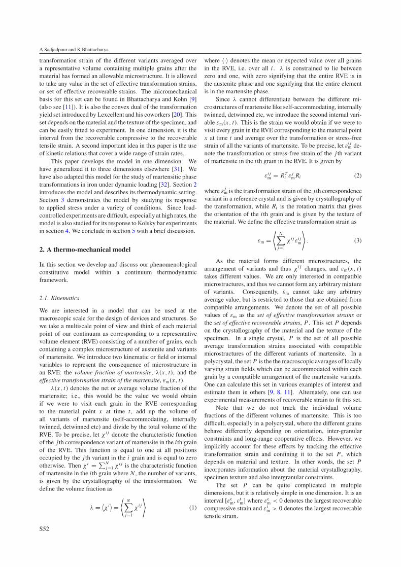
where E is the elastic modulus (assumed to be equal in both theaustenite and the martensite), ω is the difference in chemicalenergy between the austenite and the martensite, cp is the heatcapacity (assumed to be equal in both the austenite and themartensite), and ordinary thermal expansion is neglected. Thisrelation is illustrated in figure 1. We further assume that
ω(θ) = Lθcr
(θ − θcr) (20)
where L is the latent heat of transformation and θcr is thethermodynamic transformation temperature. Substituting (19)and (20) in (13), we obtain
σ = E(ε − εp − λεm), (21)
η = λLθcr
− cp
(
1 + ln
(θ
θ0
))
, (22)
dλ = σεm − ω, (23)
S53
A Sadjadpour and K Bhattacharya
Figure 1. Schematic representation of the Helmholtz energy density.
dεm = λσ, (24)
dεp = σ. (25)
The kinetic relation describing the evolution of themartensite volume fraction λ is taken to be the following:
λ =
⎧⎪⎪⎨
⎪⎪⎩
λ+(1 + (dλ − d+λ )−1)
− 1p dλ > d+
λ and λ < 1,
λ−(1 + (d−λ − dλ)
−1)− 1
p dλ < d−λ and λ > 0,
0 otherwise(26)
where λ±, d±λ , p are material parameters. This relation is
shown in figure 2. Note that the kinetic relation is characterizedby a ‘stick–slip’ character at small driving forces. The phasetransformation requires a critical driving force before it canproceed; i.e., the rate of change of volume fraction is zerofor driving forces below a critical driving force. As oneexceeds the critical driving force, note that the curve is vertical,meaning that the rate of phase transformation is indeterminateor equivalently the driving force is independent of rate ofphase transformation. This is rate-independent behavior. Thereason for this is a combination of metastability [6] and pinningby defects [1, 7, 10]. However, at large driving forces, itbecomes rate dependent and in fact asymptotes to a limitingrate. The reason for this is that phase boundaries requirean unboundedly increasing driving force for the propagationspeeds to reach towards some sound speed [10, 29]. Notethat this kinetic relation is consistent with the experimentalobservations, which say that for low driving forces, aroundd±
λ , phase transformation is rate independent [27], and at largedriving forces the material shows rate dependency [25].
The evolution of the effective transformation strain εm
describes the twinning, detwinning and other such processesthat convert one martensitic variant to another. We assume arather simple law for its evolution:
εm = Kεm(dεm, λ, εm) = α
λdεm =
{ασ εm ∈ [εc
m, εtm]
0 otherwise(27)
where α is a material parameter and is chosen large enough toguarantee a very quick process, so that εm is essentially equalto εt
m and εcm under tension and compression respectively.
Finally, we assume a rate-independent plasticity relationthat neglects the Bauschinger effect:
εp = Kεp(dεp , σy) = dεp
H=
⎧⎨
⎩
σ
Hσ � σy or σ � −σy ,
0 otherwise(28)
Figure 2. The kinetic relation between λ and the driving force dλ.
where H is the hardening parameter and σy is the plastic yieldstress.
This completes the specification of the model.
2.5. Temperature evolution
The energy balance along with the constitutive relationsdescribes the evolution of the temperature. However, this israther complicated, and therefore it is useful to make somesimplifying assumptions.
We begin by substituting for the internal energy in termsof the Helmholtz free energy and entropy in the energybalance (7) to rewrite it as
W + θη + θη = −qx + r + σ ε. (29)
Using the constitutive assumption (19) for W to expand W ,using the various definitions of driving force and simplifying,we obtain
θη = −qx + r + dλλ + dεm εm + dεp εp. (30)
Specializing now to the specific constitutive relation and inparticular (22), we obtain
cpθ = λθLθcr
− qx + r + dλλ + dεm εm + dεp εp. (31)
In the following, we shall be interested in processes wherewe can assume adiabatic conditions and neglect heat transfer(q = r = 0). Further, it turns out that the latent heatof transformation is large compared to the energy dissipatedduring transformation, martensitic variant reorientation andplasticity during typical processes of interest. Therefore, weassume
cpθ = θλLθcr
. (32)
Integrating this, we obtain a relation between temperature,volume fraction of martensite, latent heat and specific heat:
θ(t) = θ0 exp
((λ(t) − λ0)L
cpθcr
)
. (33)
3. Demonstration
We now demonstrate the model by calculating the responseof a material point to a given applied stress history, and thenconduct a parameter study.
S54
A micromechanics inspired constitutive model for shape-memory alloys: the one-dimensional case
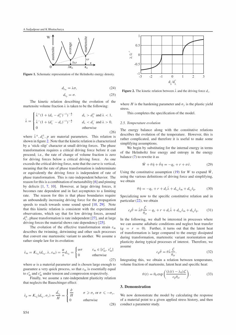
Figure 3. A typical stress–strain curve generated by the model.
3.1. Parameters
Consistent with typical experiments on NiTi (see forexample [23]), we consider the following parameters:
Ms = −51.55 ◦C and As = −6.36 ◦C
L = 79 MJ m−3 and cp = 5.4 MJ m−3 K−1
εcm = −2.5% and εt
m = 5%
E = 65 GPa and σy = 1500 MPa
(34)
where Ms and As are the martensite start and austenite starttemperatures respectively2. Recalling (26) and (23), we obtain
d+λ = −ω(Ms), d−
λ = −ω(As). (35)
Assuming further that
d+λ = −d−
λ , (36)
we conclude that
d+λ = −d−
λ = L(
As − Ms
As + Ms
)
, θcr = As + Ms
2. (37)
Note that one has to be careful to specify the absolutetemperature in kelvin to use these formulae.
We also assume the following kinetic coefficients:
λ+ = −λ− = 104, α = 1, p = 2
and H = E
50.
The parameters λ± that control the evolution rate of the volumefraction of martensite are kept fixed in the entire paper andchosen so that λ εm is smaller than ε.
Parameter α is chosen to guarantee the fast speed of theevolution of phase transformation strain εm both under tension
2 Ms is the temperature at which the specimen completely in the austenite willbegin to transform to martensite during cooling and As is the temperature atwhich the specimen completely in the martensite will begin to transform toaustenite during heating. Though stated in celsius, they have to be convertedto kelvin for use in the model.
Figure 4. Comparison between the experiment [23] and the fit to themodel.
and compression as described earlier. While larger α valuesdo not change the results, smaller α values may lead to slowevolution of εm, which is not acceptable in this setting.
The power of the kinetic law p controls the shape of itsfunction; for the given value of p = 2 its form is shown infigure 2. For higher values the kinetic relation would get closerto a Heaviside function in the first and third quadrants.
3.2. Demonstration
We consider an applied stress of the form
σ(t) = A sin ωt (38)
with A = 1300 MPa and ω = 2π/T with T = 5 ×10⁻³ s unless otherwise mentioned. In particular, this value ofloading is below the chosen yield strength, and thus plasticityis suppressed. We examine this aspect in section 3.5. Weintegrate (26)–(28), (33) as well as (21) simultaneously subjectto the initial conditions
ε(0) = 0.0%, εp(0) = 0.0%, εm(0) = 0.0%,
λ(0) = 0 and θ(0) = 22 ◦C(39)
to obtain the time trajectory of ε, εm, εp, λ and θ .The result is shown in figure 3. As we start loading,
the material deforms elastically till it reaches the point at thetop left corner of the upper flag. At this point the austeniteto martensite phase transformation starts and this results in achange of slope. It continues till the material fully transformsto martensite and we reach the top right corner of the upperflag. The material deforms elastically beyond this. As materialis unloaded, it deforms back elastically till the driving forceis equal to d−
λ at the bottom right corner of the upper flag.The reverse phase transformation starts as we traverse thelower side of the upper flag. The reverse phase transformationcontinues till material transforms back to austenite completelyat the bottom left corner of the upper flag. Material undergoesthe same process under compression; however, the bottomflag has a different shape, consistent with the well knownasymmetry of shape-memory alloys.
Figure 4 compares the stress versus strain relationobtained from experiments by McNaney et al [23] with that
S55
A Sadjadpour and K Bhattacharya
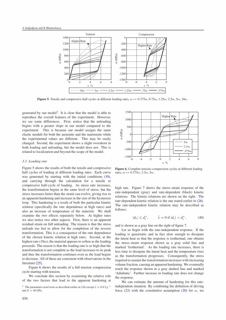
Figure 5. Tensile and compressive half-cycles at different loading rates, ω �→ 0.375ω, 0.75ω, 1.25ω, 2.5ω, 5ω, 10ω.
generated by our model3. It is clear that the model is able toreproduce the overall features of the experiment. However,we see some differences. First, notice that the unloadingbegins with a greater slope in our model compared to theexperiment. This is because our model assigns the sameelastic moduli for both the austenite and the martensite whilethe experimental values are different. This may be easilychanged. Second, the experiment shows a slight overshoot inboth loading and unloading, but the model does not. This isrelated to localization and beyond the scope of the model.
3.3. Loading rate
Figure 5 shows the results of both the tensile and compressivehalf cycles of loading at different loading rates. Each curvewas generated by starting with the initial conditions (39),and carrying through the calculation for a tensile orcompressive half-cycle of loading. As stress rate increases,the transformation begins at the same level of stress, but thestress increases faster than the strain can evolve, giving rise toan apparent hardening and increase in the size of the hysteresisloop. This hardening is a result of both the particular kineticrelation (specifically the rate dependence at high rates) andalso an increase of temperature of the material. We shallexamine the two effects separately below. At higher rateswe also notice two other aspects. First, there is an apparentresidual strain on full unloading. The reason is that the stressunloads too fast to allow for the completion of the reversetransformation. This is a consequence of the rate dependenceof the chosen kinetic relation at high rates. Second, at thehighest rate (10ω), the material appears to soften as the loadingproceeds. The reason is that the loading rate is so high that thetransformation is not complete as the load increases to its peakand thus the transformation continues even as the load beginsto decrease. All of these are consistent with observations in theliterature [25].
Figure 6 shows the results of a full tension–compressioncycle starting with tension.
We conclude this section by examining the relative roleof the two factors that lead to the apparent hardening at
3 The parameters used were as described earlier in (34) except L = 8.8 J g−1
and E = 40 GPa.
Figure 6. Complete tension–compression cycles at different loadingrates, ω �→ 0.375ω, 2.5ω, 5ω.
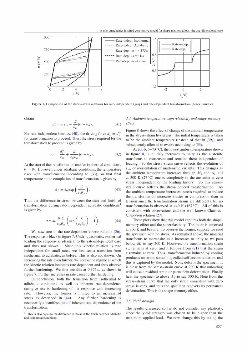
high rate. Figure 7 shows the stress–strain response of therate-independent (gray) and rate-dependent (black) kineticrelations. The kinetic relations are shown on the right. Therate-dependent kinetic relation is the one stated earlier in (26).The rate-independent kinetic relation may be described asfollows:
|dλ| � d+λ , λ = 0 if |dλ| < d+
λ , (40)
and is shown as a gray line on the right of figure 7.Let us begin with the rate-independent response. If the
loading is quasistatic and in fact slow enough to dissipatethe latent heat so that the response is isothermal, one obtainsthe stress–strain response shown as a gray solid line andmarked ‘Isothermal’. As the loading rate increases, there isless time to dissipate the latent heat and the temperature risesas the transformation progresses. Consequently, the stressrequired to sustain the transformation increases with increasingvolume fraction, causing an apparent hardening. We eventuallyreach the response shown in a gray dashed line and marked‘Adiabatic’. Further increase in loading rate does not changethe response.
We can estimate the amount of hardening for this rate-independent situation. By combining the definition of drivingforce (23) with the constitutive assumption (20) for ω, we
S56
A micromechanics inspired constitutive model for shape-memory alloys: the one-dimensional case
Figure 7. Comparison of the stress–strain relations for rate-independent (gray) and rate-dependent transformation (black) kinetics.
obtain
dλ = σεm − Lθcr
(θ − θcr). (41)
For rate-independent kinetics, (40), the driving force dλ = d+λ
for transformation to proceed. Thus, the stress required for thetransformation to proceed is given by
σ = d+λ
εm+ L
εmθcr(θ − θcr). (42)
At the start of the transformation and for isothermal conditions,θ = θ0. However, under adiabatic conditions, the temperaturerises with transformation according to (33), so that finaltemperature at the completion of transformation is given by
θ f = θ0 exp
( Lcpθcr
)
. (43)
Thus the difference in stress between the start and finish oftransformation during rate-independent adiabatic conditions4
is given by
�σ = θ0Lεmθcr
(
exp
( Lcpθcr
)
− 1
)
. (44)
We now turn to the rate-dependent kinetic relation (26).The response is black in figure 7. Under quasistatic, isothermalloading the response is identical to the rate-independent caseand thus not shown. Since this kinetic relation is rateindependent for small rates, we first see a transition fromisothermal to adiabatic, as before. This is also not shown. Onincreasing the rate even further, we access the regime at whichthe kinetic relation becomes rate dependent and thus observefurther hardening. We first see this at 0.375ω, as shown infigure 7. Further increases in rate cause further hardening.
In conclusion, both the transition from isothermal toadiabatic conditions as well as inherent rate-dependencecan give rise to hardening of the response with increasingrate. However, the former is limited to an increase ofstress as described in (44). Any further hardening isnecessarily a manifestation of inherent rate-dependence of thetransformation.4 This is also equal to the difference in stress at the finish between adiabaticand isothermal conditions.
3.4. Ambient temperature, superelasticity and shape-memoryeffect
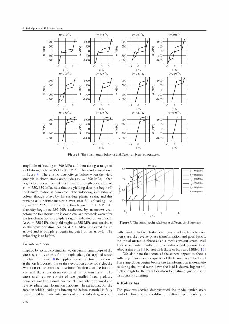
Figure 8 shows the effect of change of the ambient temperaturein the stress–strain hysteresis. The initial temperature is takento be the ambient temperature (instead of that in (39)), andsubsequently allowed to evolve according to (33).
At 200 K (−73 ◦C), the lowest ambient temperature shownin figure 8, λ quickly increases to unity as the austenitetransforms to martensite and remains there independent ofloading. So the stress–strain curve reflects the evolution ofεm, or reorientation of martensitic variants. This changes asthe ambient temperature increases through Ms and As, tillat 300 K (27 ◦C) one is completely in the austenite at zerostress independent of the loading history. So this stress–strain curve reflects the stress-induced transformation. Asthe ambient temperature increases, stress required to inducethe transformation increases (faster in compression than intension since the transformation strains are different), till notransformation is observed at 440 K (167 ◦C). All of this isconsistent with observations and the well known Clausius–Clapeyron relation [27].
These plots show that this model captures both the shape-memory effect and the superelasticity. The latter is observedat 300 K and beyond. To observe the former, suppose we coolthe specimen with no stress. As remarked above, the materialtransforms to martensite as λ increases to unity as we passbelow Ms to say 200 K. However, the transformation strainεm remains at zero, and it follows from (21) that the strainε remains at zero. Thus, transformation induced by coolingproduces no strain, something called self-accommodation, andthis is captured by the model. Now, deform the specimen. Itis clear from the stress–strain curve at 200 K that unloadingwill cause a residual strain or permanent deformation. Finallyheat the specimen to above A f to say 300 K. Note from thestress–strain curve that the only strain consistent with zerostress is zero, and thus the specimen recovers its permanentdeformation. This is the shape-memory effect.
3.5. Yield strength
The results discussed so far do not consider any plasticity,since the yield strength was chosen to be higher than themaximum applied load. We now change this by taking the
S57
A Sadjadpour and K Bhattacharya
Figure 8. The strain–strain behavior at different ambient temperatures.
amplitude of loading to 800 MPa and then taking a range ofyield strengths from 350 to 850 MPa. The results are shownin figure 9. There is no plasticity as before when the yieldstrength is above stress amplitude (σy = 850 MPa). Onebegins to observe plasticity as the yield strength decreases. Atσy = 750, 650 MPa, note that the yielding does not begin tillthe transformation is complete. The unloading is similar asbefore, though offset by the residual plastic strain, and thisremains as a permanent strain even after full unloading. Atσy = 550 MPa, the transformation begins at 500 MPa; theplasticity begins at 550 MPa (indicated by an arrow) evenbefore the transformation is complete, and proceeds even afterthe transformation is complete (again indicated by an arrow).At σy = 350 MPa, the yield begins at 350 MPa, and continuesas the transformation begins at 500 MPa (indicated by anarrow) and is complete (again indicated by an arrow). Theunloading is as before.
3.6. Internal loops
Inspired by some experiments, we discuss internal loops of thestress–strain hysteresis for a simple triangular applied stressfunction. In figure 10 the applied stress function σ is shownat the top left corner, the strain ε evolution at the top right, theevolution of the martensitic volume fraction λ at the bottomleft, and the stress strain curves at the bottom right. Thestress–strain curves consist of two parallel, linearly elasticbranches and two almost horizontal lines where forward andreverse phase transformation happens. In particular, for thecases in which loading is interrupted before material is fullytransformed to martensite, material starts unloading along a
Figure 9. The stress–strain relations at different yield strengths.
path parallel to the elastic loading–unloading branches andthen starts the reverse phase transformation and goes back tothe initial austenite phase at an almost constant stress level.This is consistent with the observations and arguments ofAbeyaratne et al [1] but not with those of Huo and Muller [16].
We also note that some of the curves appear to show asoftening. This is a consequence of the triangular applied load.The ramp-down begins before the transformation is complete,so during the initial ramp-down the load is decreasing but stillhigh enough for the transformation to continue, giving rise toan apparent softening.
4. Kolsky bar
The previous section demonstrated the model under stresscontrol. However, this is difficult to attain experimentally. In
S58
A micromechanics inspired constitutive model for shape-memory alloys: the one-dimensional case
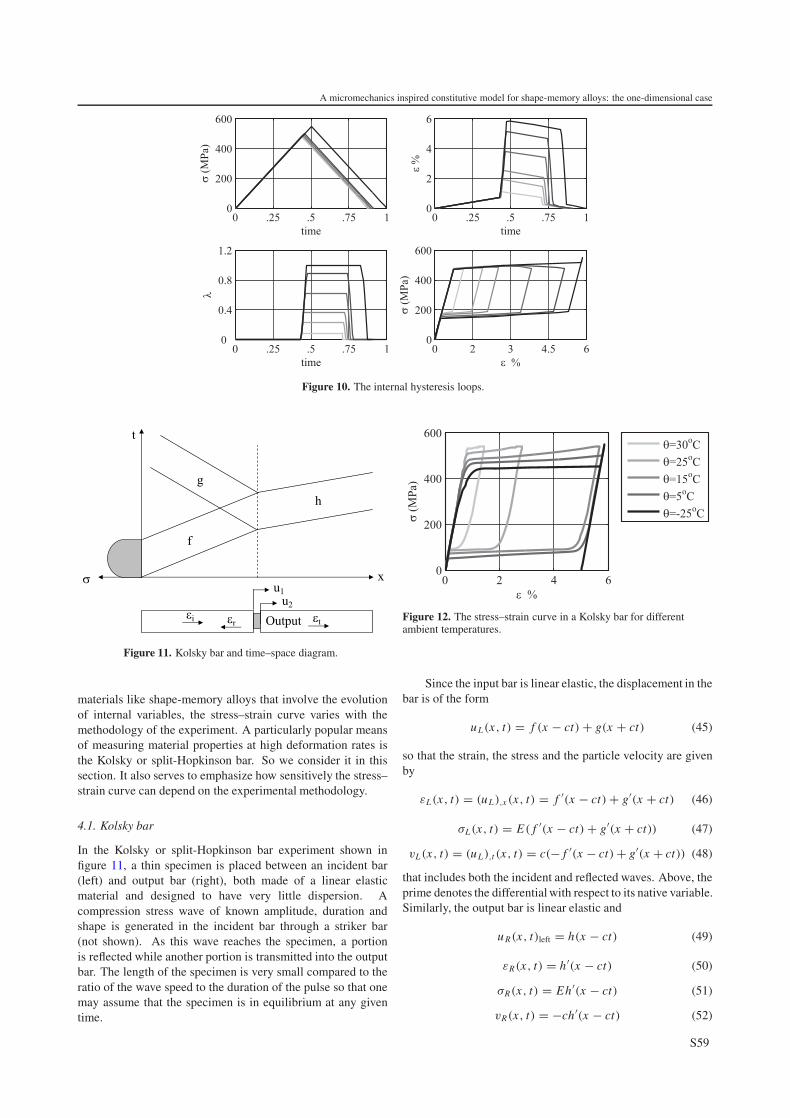
Figure 10. The internal hysteresis loops.
Figure 11. Kolsky bar and time–space diagram.
materials like shape-memory alloys that involve the evolutionof internal variables, the stress–strain curve varies with themethodology of the experiment. A particularly popular meansof measuring material properties at high deformation rates isthe Kolsky or split-Hopkinson bar. So we consider it in thissection. It also serves to emphasize how sensitively the stress–strain curve can depend on the experimental methodology.
4.1. Kolsky bar
In the Kolsky or split-Hopkinson bar experiment shown infigure 11, a thin specimen is placed between an incident bar(left) and output bar (right), both made of a linear elasticmaterial and designed to have very little dispersion. Acompression stress wave of known amplitude, duration andshape is generated in the incident bar through a striker bar(not shown). As this wave reaches the specimen, a portionis reflected while another portion is transmitted into the outputbar. The length of the specimen is very small compared to theratio of the wave speed to the duration of the pulse so that onemay assume that the specimen is in equilibrium at any giventime.
Figure 12. The stress–strain curve in a Kolsky bar for differentambient temperatures.
Since the input bar is linear elastic, the displacement in thebar is of the form
uL(x, t) = f (x − ct) + g(x + ct) (45)
so that the strain, the stress and the particle velocity are givenby
that includes both the incident and reflected waves. Above, theprime denotes the differential with respect to its native variable.Similarly, the output bar is linear elastic and
u R(x, t)left = h(x − ct) (49)
εR(x, t) = h ′(x − ct) (50)
σR(x, t) = Eh ′(x − ct) (51)
vR(x, t) = −ch ′(x − ct) (52)
S59
A Sadjadpour and K Bhattacharya
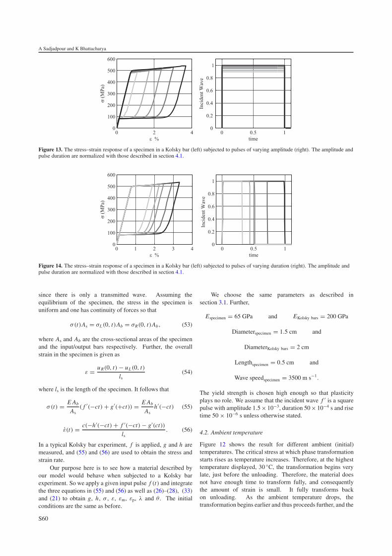
Figure 13. The stress–strain response of a specimen in a Kolsky bar (left) subjected to pulses of varying amplitude (right). The amplitude andpulse duration are normalized with those described in section 4.1.
Figure 14. The stress–strain response of a specimen in a Kolsky bar (left) subjected to pulses of varying duration (right). The amplitude andpulse duration are normalized with those described in section 4.1.
since there is only a transmitted wave. Assuming theequilibrium of the specimen, the stress in the specimen isuniform and one has continuity of forces so that
σ(t)As = σL (0, t)Ab = σR(0, t)Ab, (53)
where As and Ab are the cross-sectional areas of the specimenand the input/output bars respectively. Further, the overallstrain in the specimen is given as
ε = u R(0, t) − uL(0, t)
ls(54)
where ls is the length of the specimen. It follows that
σ(t) = E Ab
As( f ′(−ct) + g′(+ct)) = E Ab
Ash ′(−ct) (55)
ε(t) = c(−h ′(−ct) + f ′(−ct) − g′(ct))
ls. (56)
In a typical Kolsky bar experiment, f is applied, g and h aremeasured, and (55) and (56) are used to obtain the stress andstrain rate.
Our purpose here is to see how a material described byour model would behave when subjected to a Kolsky barexperiment. So we apply a given input pulse f (t) and integratethe three equations in (55) and (56) as well as (26)–(28), (33)and (21) to obtain g, h, σ , ε, εm, εp, λ and θ . The initialconditions are the same as before.
We choose the same parameters as described insection 3.1. Further,
Especimen = 65 GPa and EKolsky bars = 200 GPa
Diameterspecimen = 1.5 cm and
DiameterKolsky bars = 2 cm
Lengthspecimen = 0.5 cm and
Wave speedspecimen = 3500 m s−1.
The yield strength is chosen high enough so that plasticityplays no role. We assume that the incident wave f ′ is a squarepulse with amplitude 1.5 × 10⁻³, duration 50 × 10−4 s and risetime 50 × 10−6 s unless otherwise stated.
4.2. Ambient temperature
Figure 12 shows the result for different ambient (initial)temperatures. The critical stress at which phase transformationstarts rises as temperature increases. Therefore, at the highesttemperature displayed, 30 ◦C, the transformation begins verylate, just before the unloading. Therefore, the material doesnot have enough time to transform fully, and consequentlythe amount of strain is small. It fully transforms backon unloading. As the ambient temperature drops, thetransformation begins earlier and thus proceeds further, and the
S60
A micromechanics inspired constitutive model for shape-memory alloys: the one-dimensional case
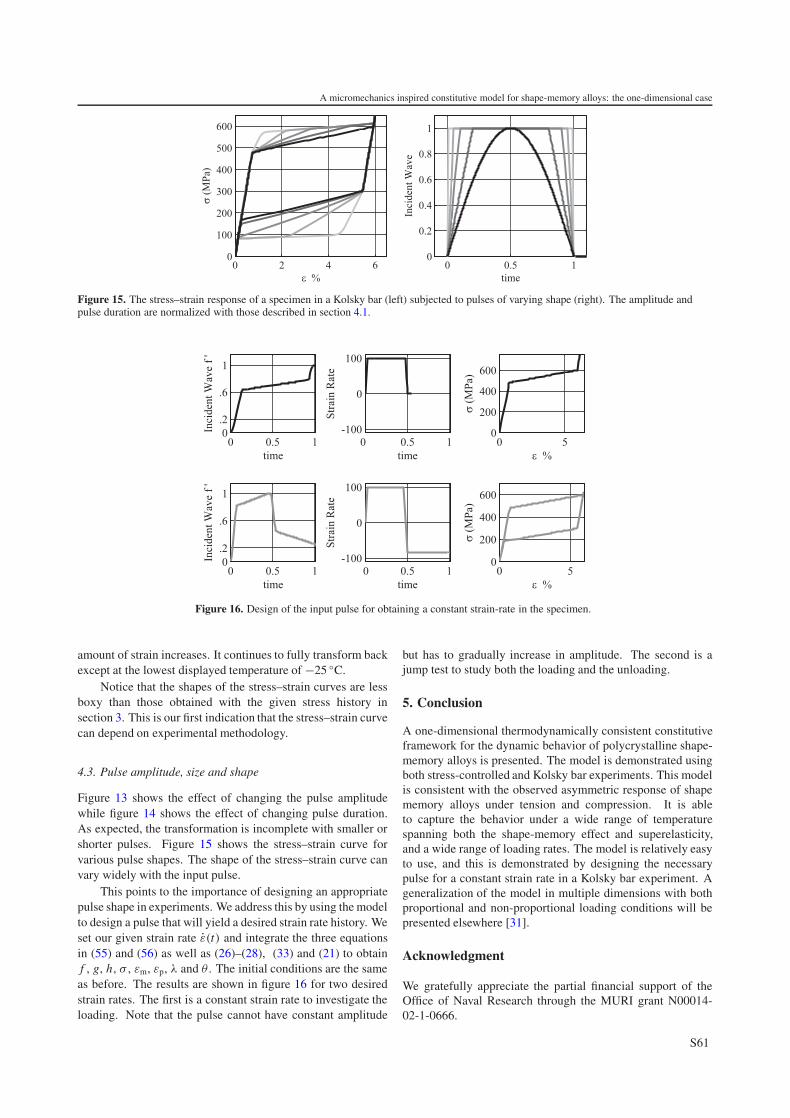
Figure 15. The stress–strain response of a specimen in a Kolsky bar (left) subjected to pulses of varying shape (right). The amplitude andpulse duration are normalized with those described in section 4.1.
Figure 16. Design of the input pulse for obtaining a constant strain-rate in the specimen.
amount of strain increases. It continues to fully transform backexcept at the lowest displayed temperature of −25 ◦C.
Notice that the shapes of the stress–strain curves are lessboxy than those obtained with the given stress history insection 3. This is our first indication that the stress–strain curvecan depend on experimental methodology.
4.3. Pulse amplitude, size and shape
Figure 13 shows the effect of changing the pulse amplitudewhile figure 14 shows the effect of changing pulse duration.As expected, the transformation is incomplete with smaller orshorter pulses. Figure 15 shows the stress–strain curve forvarious pulse shapes. The shape of the stress–strain curve canvary widely with the input pulse.
This points to the importance of designing an appropriatepulse shape in experiments. We address this by using the modelto design a pulse that will yield a desired strain rate history. Weset our given strain rate ε(t) and integrate the three equationsin (55) and (56) as well as (26)–(28), (33) and (21) to obtainf , g, h, σ , εm, εp, λ and θ . The initial conditions are the sameas before. The results are shown in figure 16 for two desiredstrain rates. The first is a constant strain rate to investigate theloading. Note that the pulse cannot have constant amplitude
but has to gradually increase in amplitude. The second is ajump test to study both the loading and the unloading.
5. Conclusion
A one-dimensional thermodynamically consistent constitutiveframework for the dynamic behavior of polycrystalline shape-memory alloys is presented. The model is demonstrated usingboth stress-controlled and Kolsky bar experiments. This modelis consistent with the observed asymmetric response of shapememory alloys under tension and compression. It is ableto capture the behavior under a wide range of temperaturespanning both the shape-memory effect and superelasticity,and a wide range of loading rates. The model is relatively easyto use, and this is demonstrated by designing the necessarypulse for a constant strain rate in a Kolsky bar experiment. Ageneralization of the model in multiple dimensions with bothproportional and non-proportional loading conditions will bepresented elsewhere [31].
Acknowledgment
We gratefully appreciate the partial financial support of theOffice of Naval Research through the MURI grant N00014-02-1-0666.
S61
A Sadjadpour and K Bhattacharya
References
[1] Abeyaratne R, Chu C and James R D 1996 Kinetics ofmaterials with wiggly energies: theory and application to theevolution of twinning microstructure in a Cu–Al–Ni alloyPhil. Mag. A 73 457–97
[2] Abeyaratne R and Knowles J K 1993 A continuum model of athermoelastic solid capable of undergoing phase-transitionsJ. Mech. Phys. Solids 41 541–71
[3] Auricchio F, Taylor R L and Lubliner J 1997 Shape-memoryalloys: macromodelling and numerical simulations of thesuperelastic behavior Comput. Meth. Appl. Mech. Eng.146 281–312
[4] Auricchio F and Petrini L 2004 A three-dimensional modeldescribing stress-temperature induced solid phasetransformations: solution algorithm and boundary valueproblems Int. J. Numer. Methods Eng. 61 807–36
[5] Ball J M and James R D 1987 Fine phase mixtures asminimizers of energy Arch. Ration. Mech. Anal. 100 13–52
[6] Ball J M, Chu C and James R D 1995 Hysteresis duringstress-induced variant rearrangement J. Physique Coll.5 245–51
[7] Bhattacharya K 1999 Phase boundary propagation inheterogeneous bodies Proc. R. Soc. A 455 757–66
[8] Bhattacharya K 2003 Microstructure of Martensite (Oxford:Oxford University Press)
[9] Bhattacharya K and Kohn R V 1997 Energy minimization andthe recoverable strains of polycrystalline shape-memoryalloys Arch. Ration. Mech. Anal. 139 99–180
[10] Bhattacharya K, Purohit P and Craciun B 2003 The mobility oftwin and phase boundaries J. Physique Coll. 112 163–6
[11] Bhattacharya K and Schlomerkemper A 2004 Transformationyield surface of shape-memory alloys J. Physique Coll.115 155–62
[12] Bhattacharyya A, Lagoudas D C, Wang Y and Kinra V K 1995On the role of thermoelectric heat transfer in the design ofSMA actuators: theoretical modelling and experimentsSmart Mater. Struct. 4 252–63
[13] Boyd J G and Lagoudas D C 1996 A thermodynamicconstitutive model for shape memory materials: 1. Themonolithic shape memory alloy Int. J. Plast. 12 843–73
[14] Brocca M, Brinson L C and Bazant Z 2002 Three-dimensionalconstitutive model for shape memory alloys based onmicroplane J. Mech. Phys. Solids 50 1051–77
[15] Coleman B D and Noll W 1963 The thermodynamics of elasticmaterials with heat conduction and viscosity Arch. Ration.Mech. Anal. 13 167–83
[16] Huo Y and Muller I 1993 Nonequilibrium thermodynamics ofpseudoelasticity Cont. Mech. Thermodyn. 5 163–204
[17] Huang M and Brinson L C 1998 Multivariant model for singlecrystal shape memory alloy behavior J. Mech. Phys. Solids46 1379–409
[18] Jung Y J, Papadopoulos P and Ritchie R O 2004 Constitutivemodelling and numerical simulation of multivariant phasetransformation in superelastic shape-memory alloys Int. J.Numer. Methods Eng. 60 429–60
[19] Lexcellent C, Goo B C, Sun Q P and Bernardini J 1996Characterization, thermomechanical behaviour andmicromechanical-based constitutive model of shape-memoryCu–Zn–Al single crystals Acta Mater. 44 3773–80
[20] Lexcellent C, Vivet A, Bouvet C, Calloch S and Blanc P 2002Experimental and numerical determinations of the initial
surface of phase transformation under biaxial polycrystallineshape-memory alloys J. Mech. Phys. Solids 50 2717–35
[21] Lu Z K and Weng G J 1997 Martensitic transformation andstress–strain relations of shape-memory alloys J. Mech.Phys. Solids 45 1905
[22] Marketz F and Fischer F D 1996 Modelling the mechanicalbehavior of shape memory alloys under variant coalescenceComput. Mater. Sci. 5 210–26
[23] McNaney J M, Imbeni V, Jung Y, Papadopoulos P andRitchie R O 2003 An experimental study of the superelasticeffect in a shape-memory Nitinol alloy under biaxial loadingMech. Mater. 35 969–86
[24] Naito H, Matsuzaki Y and Ikeda T 2004 A unified constitutivemodel of phase transformations and rearrangements of shapememory alloy wires subjected to quasistatic load SmartMater. Struct. 13 535–43
[25] Nemat-Nasser S, Choi J Y, Guo W G, Isaacs J B andTaya M 2005 High strain-rate, small strain response of aNiTi shape-memory alloy J. Eng. Mater. Technol. 127 83–9
[26] Niclaeys C, Ben Zineb T, Arbab-Chirani S and Patoor E 2002Determination of the interaction energy in the martensiticstate Int. J. Plast. 18 1619–47
[27] Otsuka K and Wayman C M 1998 Shape Memory Materials(Cambridge: Cambridge University Press)
[28] Paiva A, Savi M A, Braga A M B and Pacheco P M C L 2005A constitutive model for shape memory alloys consideringtensile-compressive asymmetry and plasticity Int. J. SolidStruct. 42 3439–57
[29] Purohit P K 2002 Dynamics of phase transformations in strings,beams and atomic chains PhD Thesis California Institute ofTechnology
[30] Qidwai M A and Lagoudas D C 2000 Numericalimplementation of a shape memory alloy thermomechanicalconstitutive model using return mapping algorithms Int. J.Numer. Methods Eng. 47 1123–68
[31] Sadjadpour A and Bhattacharya K 2006 A micromechanicsinspired constitutive model for shape-memory alloys, inpreparation
[32] Sadjadpour A, Rittel D, Ravichandran G andBhattacharya K 2006 Dynamic deformation of iron undershear, in preparation
[33] Stoijov V and Bhattacharyya A 2002 A theoretical frameworkof one-dimensional sharp phase fronts in shape memoryalloys Acta Mater. 50 4939–52
[34] Sun Q P and Hwang K C 1993 Micromechanics modeling forthe constitutive behavior of polycrystalline shape-memoryalloys: 1. Derivation of general relations J. Mech. Phys.Solids 41 1–17
Sun Q P and Hwang K C 1993 Micromechanics modeling forthe constitutive behavior of polycrystalline shape-memoryalloys: 2. Study of individual phenomena J. Mech. Phys.Solids 41 19–33
[35] Thamburaja P and Anand L 2001 Polycrystallineshape-memory materials: effect of crystallographic textureJ. Mech. Phys. Solids 49 709–37
[36] Wang Y H and Fang D N 2003 A three-dimensionalconstitutive model for shape memory alloys Int. J. NonlinearSci. Numer. Sim. 4 81–7
[37] Zhu J J, Huang N G, Liew K M and Zhu Z H 2002 Athermodynamic constitutive model for stress induced phasetransformation in shape memory alloys Int. J. Solid Struct.39 741–63


![Effects of Lay-Up Sequence and Widths on The SERR of ...web.deu.edu.tr/fmd/s62/S62-m5.pdf[22] ASTM D3518/D3518M−13 [23], respectively. Specimens were prepared according to the ASTM](https://static.documents.pub/doc/80x56/6149abbb12c9616cbc68e97f/effects-of-lay-up-sequence-and-widths-on-the-serr-of-webdeuedutrfmds62s62-m5pdf.jpg)


