IBM Cognos 8 - WordPress.com · Chapter1:GuidelinesforModelingMetadata Framework Manager is a...

IBM® Cognos® 8

FRAMEWORK MANAGER

GUIDELINES FOR MODELING METADATA

Product InformationThis document applies to IBM® Cognos® 8 Version 8.4 and may also apply to subsequent releases. To check for newer versions of this document,visit the IBM Cognos Resource Center (http://www.ibm.com/software/data/support/cognos_crc.html).

CopyrightCopyright © 2008 Cognos ULC (formerly Cognos Incorporated). Cognos ULC is an IBM Company.Portions of Cognos ULC software products are protected by one or more of the following U.S. Patents: 6,609,123 B1; 6,611,838 B1; 6,662,188B1; 6,728,697 B2; 6,741,982 B2; 6,763,520 B1; 6,768,995 B2; 6,782,378 B2; 6,847,973 B2; 6,907,428 B2; 6,853,375 B2; 6,986,135 B2;6,995,768 B2; 7,062,479 B2; 7,072,822 B2; 7,111,007 B2; 7,130,822 B1; 7,155,398 B2; 7,171,425 B2; 7,185,016 B1; 7,213,199 B2; 7,243,106B2; 7,257,612 B2; 7,275,211 B2; 7,281,047 B2; 7,293,008 B2; 7,296,040 B2; 7,318,058 B2; 7,325,003 B2; 7,333,995 B2.Cognos and the Cognos logo are trademarks of Cognos ULC (formerly Cognos Incorporated) in the United States and/or other countries. IBMand the IBM logo are trademarks of International Business Machines Corporation in the United States, or other countries or both. Java andall Java-based trademarks are trademarks of Sun Microsystems, Inc. in the United States, other countries, or both. Other company, product,or service names may be trademarks or service marks of others.While every attempt has been made to ensure that the information in this document is accurate and complete, some typographical errors ortechnical inaccuracies may exist. Cognos does not accept responsibility for any kind of loss resulting from the use of information containedin this document.This document shows the publication date. The information contained in this document is subject to change without notice. Any improvementsor changes to the information contained in this document will be documented in subsequent editions.U.S. Government Restricted Rights. The software and accompanying materials are provided with Restricted Rights. Use, duplication, or dis-closure by the Government is subject to the restrictions in subparagraph (C)(1)(ii) of the Rights in Technical Data and Computer clause atDFARS 252.227-7013, or subparagraphs (C)(1) and (2) of the Commercial Computer Software - Restricted Rights at 48CFR52.227 as applicable.The Contractor is Cognos Corporation, 15 Wayside Road, Burlington, MA 01803.This document contains proprietary information of Cognos. All rights are reserved. No part of this document may be copied, photocopied,reproduced, stored in a retrieval system, transmitted in any form or by any means, or translated into another language without the priorwritten consent of Cognos.

http://www.ibm.com/software/data/support/cognos_crc.html

Table of Contents

Chapter 1: Guidelines for Modeling Metadata 5Understanding IBM Cognos 8 Modeling Concepts 5

Relational Modeling Concepts 6Model Design Considerations 15Dimensional Modeling Concepts 22

Building the Relational Model 23Defining the Relational Modeling Foundation 24Defining the Dimensional Representation of the Model 30Organizing the Model 33

Chapter 2: The SQL Generated by IBM Cognos 8 37Understanding Dimensional Queries 37

Single Fact Query 37Multiple-fact, Multiple-grain Query on Conformed Dimensions 38Modeling 1-n Relationships as 1-1 Relationships 41Multiple-fact, Multiple-grain Query on Non-Conformed Dimensions 43

Resolving Ambiguously Identified Dimensions and Facts 46Query Subjects That Represent a Level of Hierarchy 46Resolving Queries That Should Not Have Been Split 47

Index 51

Guidelines for Modeling Metadata 3

4 Framework Manager

Table of Contents

Chapter 1: Guidelines for Modeling Metadata

Framework Manager is a metadata modeling tool that drives query generation for IBM Cognos 8.

A model is a collection of metadata that includes physical information and business information

for one or more data sources. IBM Cognos 8 enables performance management on normalized and

denormalized relational data sources as well as a variety of OLAP data sources.

The first section of this document discusses fundamental IBM Cognos 8 modeling concepts that

you need to understand about modeling metadata for use in business reporting and analysis (p. 5).

The next section discusses building the relational model (p. 23).

To access this document in a different language, go to installation location\cognos\c8\webcontent\

documentation and open the folder for the language you want. Then open ug_best.pdf.

Understanding IBM Cognos 8 Modeling ConceptsBefore you begin, there are concepts that you need to understand.

Relational modeling concepts:

● cardinality (p. 6)

● determinants (p. 8)

● multiple-fact, multiple-grain queries (p. 12)

Model design considerations:

● relationships and determinants (p. 15)

● minimized SQL (p. 16)

● metadata caching (p. 17)

● query subjects vs. dimensions (p. 18)

● shortcuts vs. copies of query subjects (p. 18)

● folders vs. namespaces (p. 20)

● order of operations (p. 20)

● impact of model size(p. 22)

Dimensional modeling concepts:

● regular dimensions (p. 22)

● measure dimensions (p. 23)

● scope relationships (p. 23)


Relational Modeling ConceptsWhen modeling in Framework Manager, it is important to understand that there is no requirement

to design your data source to be a perfect star schema. Snowflaked and other forms of normalized

schemas are equally acceptable as long as your data source is optimized to deliver the performance

you require for your application. In general, we recommend that you create a logical model that

conforms to star schema concepts. This is a requirement for Analysis Studio and has also proved

to be an effective way to organize data for your users.

When beginning to develop your application with a complex data source, it is recommended that

you create a simplified view that represents how your users view the business and that is designed

using the guidelines in this document to deliver predictable queries and results. A well-built relational

model acts as the foundation of your application and provides you with a solid starting point if

you choose to take advantage of dimensional capabilities in IBM Cognos 8.

If you are starting with a star schema data source, less effort is required to model because the concepts

employed in creating a star schema lend themselves well to building applications for query and

analysis. The guidelines in this document will assist you in designing a model that will meet the

needs of your application.

Cardinality

Relationships exist between two query subjects. The cardinality of a relationship is the number of

related rows for each of the two query subjects. The rows are related by the expression of the rela-

tionship; this expression usually refers to the primary and foreign keys of the underlying tables.

IBM Cognos 8 uses the cardinality of a relationship in the following ways:

● to avoid double-counting fact data

● to support loop joins that are common in star schema models

● to optimize access to the underlying data source system

● to identify query subjects that behave as facts or dimensions

A query that uses multiple facts from different underlying tables is split into separate queries for

each underlying fact table. Each single fact query refers to its respective fact table as well as to the

dimensional tables related to that fact table. Another query is used to merge these individual queries

into one result set. This latter operation is generally referred to as a stitched query. You know that

you have a stitched query when you see coalesce and a full outer join.

A stitched query also allows IBM Cognos 8 to properly relate data at different levels of granularity

(p. 12).

Cardinality in Generated Queries

IBM Cognos 8 supports both minimum-maximum cardinality and optional cardinality.

In 0:1, 0 is the minimum cardinality, 1 is the maximum cardinality.

In 1:n , 1 is the minimum cardinality, n is the maximum cardinality.

A relationship with cardinality specified as 1:1 to 1:n is commonly referred to as 1 to n when

focusing on the maximum cardinalities.

6 Framework Manager


A minimum cardinality of 0 indicates that the relationship is optional. You specify a minimum

cardinality of 0 if you want the query to retain the information on the other side of the relationship

in the absence of a match. For example, a relationship between customer and actual sales may be

specified as 1:1 to 0:n. This indicates that reports will show the requested customer information

even though there may not be any sales data present.

Therefore a 1 to n relationship can also be specified as:

● 0:1 to 0:n

● 0:1 to 1:n

● 1:1 to 0:n

● 1:1 to 1:n

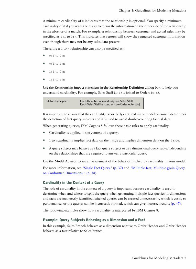
Use the Relationship impact statement in the Relationship Definition dialog box to help you

understand cardinality. For example, Sales Staff (1:1) is joined to Orders (0:n).

It is important to ensure that the cardinality is correctly captured in the model because it determines

the detection of fact query subjects and it is used to avoid double-counting factual data.

When generating queries, IBM Cognos 8 follows these basic rules to apply cardinality:

● Cardinality is applied in the context of a query.

● 1 to ncardinality implies fact data on the n side and implies dimension data on the 1 side.

● A query subject may behave as a fact query subject or as a dimensional query subject, depending

on the relationships that are required to answer a particular query.

Use the Model Advisor to see an assessment of the behavior implied by cardinality in your model.

For more information, see "Single Fact Query" (p. 37) and "Multiple-fact, Multiple-grain Query

on Conformed Dimensions " (p. 38).

Cardinality in the Context of a Query

The role of cardinality in the context of a query is important because cardinality is used to

determine when and where to split the query when generating multiple-fact queries. If dimensions

and facts are incorrectly identified, stitched queries can be created unnecessarily, which is costly to

performance, or the queries can be incorrectly formed, which can give incorrect results (p. 47).

The following examples show how cardinality is interpreted by IBM Cognos 8.

Example: Query Subjects Behaving as a Dimension and a Fact

In this example, Sales Branch behaves as a dimension relative to Order Header and Order Header

behaves as a fact relative to Sales Branch.



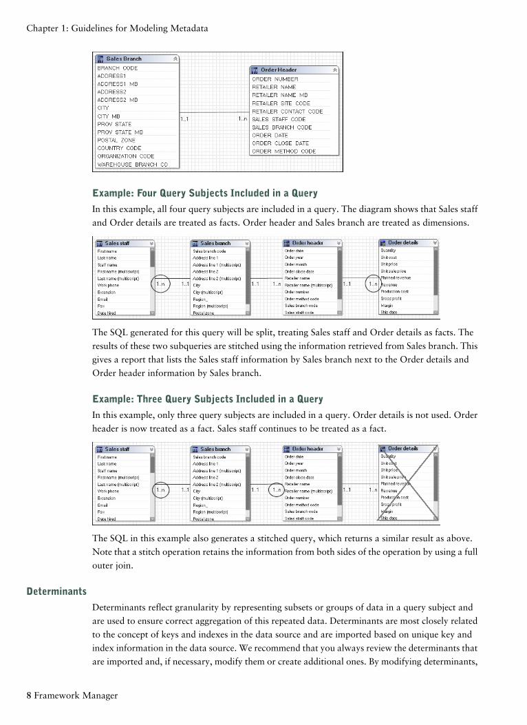
Example: Four Query Subjects Included in a Query

In this example, all four query subjects are included in a query. The diagram shows that Sales staff

and Order details are treated as facts. Order header and Sales branch are treated as dimensions.

The SQL generated for this query will be split, treating Sales staff and Order details as facts. The

results of these two subqueries are stitched using the information retrieved from Sales branch. This

gives a report that lists the Sales staff information by Sales branch next to the Order details and

Order header information by Sales branch.

Example: Three Query Subjects Included in a Query

In this example, only three query subjects are included in a query. Order details is not used. Order

header is now treated as a fact. Sales staff continues to be treated as a fact.

The SQL in this example also generates a stitched query, which returns a similar result as above.

Note that a stitch operation retains the information from both sides of the operation by using a full

outer join.

Determinants

Determinants reflect granularity by representing subsets or groups of data in a query subject and

are used to ensure correct aggregation of this repeated data. Determinants are most closely related

to the concept of keys and indexes in the data source and are imported based on unique key and

index information in the data source. We recommend that you always review the determinants that

are imported and, if necessary, modify them or create additional ones. By modifying determinants,

8 Framework Manager


you can override the index and key information in your data source, replacing it with information

that is better aligned with your reporting and analysis needs. By adding determinants, you can

represent groups of repeated data that are relevant for your application.

An example of a unique determinant is Day in the Time example below. An example of a non-

unique determinant is Month; the key in Month is repeated for the number of days in a particular

month. When you define a non-unique determinant, you should specify group by. This indicates

to IBM Cognos 8 that when the keys or attributes associated with that determinant are repeated

in the data, it should apply aggregate functions and grouping to avoid double-counting. It is not

recommended that you specify determinants that have both uniquely identified and group by

selected or have neither selected.

Day NameDay KeyMonth NameMonth KeyYear Key

Sunday, January 1, 200620060101January 062006012006

Monday, January 2, 200620060102January 062006012006

You can define three determinants for this data set as follows -- two group by determinants (Year

and Month) and one unique determinant (Day). The concept is similar but not identical to the

concept of levels and hierarchies.

Group ByUniquely IdentifiedAttributesKeyName of theDeterminant

YesNoNoneYear KeyYear

YesNoMonth NameMonth KeyMonth

NoYesDay NameDay KeyDay

Month Key

Month Name

Year Key

In this case, we use only one key for each determinant because each key contains enough information

to identify a group within the data. Often Month is a challenge if the key does not contain enough

information to clarify which year the month belongs to. In this case, however, the Month key

includes the Year key and so, by itself, is enough to identify months as a sub-grouping of years.

Note: While you can create a determinant that groups months without the context of years, this is

a less common choice for reporting because all data for February of all years would be grouped

together instead of all data for February 2006 being grouped together.

Using Determinants with Multiple-Part Keys

In the Time dimension example above, one key was sufficient to identify each set of data for a

determinant but that is not always the case.



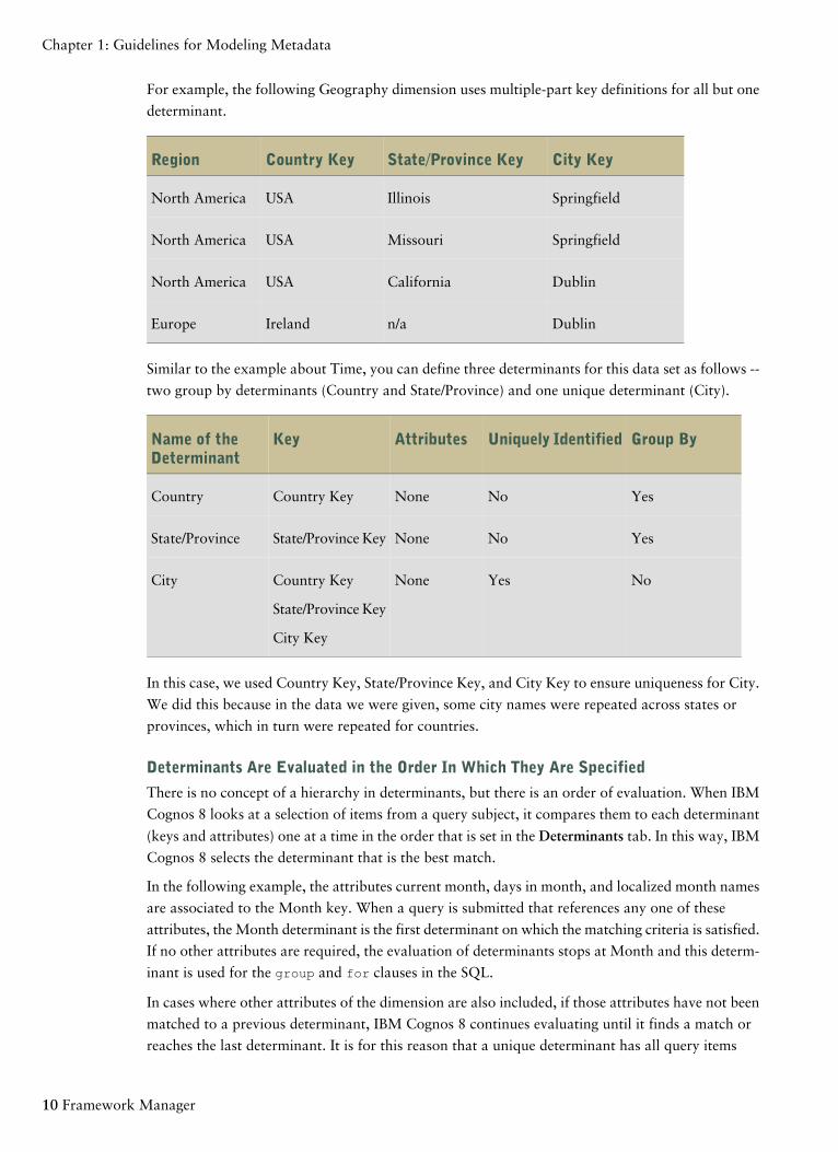
For example, the following Geography dimension uses multiple-part key definitions for all but one

determinant.

City KeyState/Province KeyCountry KeyRegion

SpringfieldIllinoisUSANorth America

SpringfieldMissouriUSANorth America

DublinCaliforniaUSANorth America

Dublinn/aIrelandEurope

Similar to the example about Time, you can define three determinants for this data set as follows --

two group by determinants (Country and State/Province) and one unique determinant (City).

Group ByUniquely IdentifiedAttributesKeyName of theDeterminant

YesNoNoneCountry KeyCountry

YesNoNoneState/Province KeyState/Province

NoYesNoneCountry KeyCity

State/Province Key

City Key

In this case, we used Country Key, State/Province Key, and City Key to ensure uniqueness for City.

We did this because in the data we were given, some city names were repeated across states or

provinces, which in turn were repeated for countries.

Determinants Are Evaluated in the Order In Which They Are Specified

There is no concept of a hierarchy in determinants, but there is an order of evaluation. When IBM

Cognos 8 looks at a selection of items from a query subject, it compares them to each determinant

(keys and attributes) one at a time in the order that is set in the Determinants tab. In this way, IBM

Cognos 8 selects the determinant that is the best match.

In the following example, the attributes current month, days in month, and localized month names

are associated to the Month key. When a query is submitted that references any one of these

attributes, the Month determinant is the first determinant on which the matching criteria is satisfied.

If no other attributes are required, the evaluation of determinants stops at Month and this determ-

inant is used for the group and for clauses in the SQL.

In cases where other attributes of the dimension are also included, if those attributes have not been

matched to a previous determinant, IBM Cognos 8 continues evaluating until it finds a match or

reaches the last determinant. It is for this reason that a unique determinant has all query items

10 Framework Manager


associated to it. If no other match is found, the unique key of the entire data set is used to determine

how the data is grouped.

When to Use Determinants

While determinants can be used to solve a variety of problems related to data granularity, you

should always use them in the following primary cases:

● A query subject that behaves as a dimension has multiple levels of granularity and will be joined

on different sets of keys to fact data.

For example, Time has multiple levels, and it is joined to Inventory on the Month Key and to

Sales on the Day Key. For more information, see "Multiple-fact, Multiple-grain Queries" (p. 12).

● There is a need to count or perform other aggregate functions on a key or attribute that is

repeated.

For example, Time has a Month Key and an attribute, Days in the month, that is repeated for

each day. If you want to use Days in the month in a report, you do not want the sum of Days

in the month for each day in the month. Instead, you want the unique value of Days in the

month for the chosen Month Key. In SQL, that is XMIN(Days in the month for Month_Key).

There is also a Group by clause in the Cognos SQL.

There are less common cases when you need to use determinants:

● You want to uniquely identify the row of data when retrieving text BLOB data from the data

source.

Querying blobs requires additional key or index type information. If this information is not

present in the data source, you can add it using determinants. Override the determinants

imported from the data source that conflict with relationships created for reporting.



You cannot use multiple-segment keys when the query subject accesses blob data. With summary

queries, blob data must be retrieved separately from the summary portion of the query. To do

this, you need a key that uniquely identifies the row and the key must not have multiple segments.

● A join is specified that uses fewer keys than a unique determinant that is specified for a query

subject.

If your join is built on a subset of the columns that are referenced by the keys of a unique

determinant on the 0..1 or 1..1 side of the relationships, there will be a conflict. Resolve this

conflict by modifying the relationship to fully agree with the determinant or by modifying the

determinant to support the relationship.

● You want to override the determinants imported from the data source that conflict with rela-

tionships created for reporting.

For example, there are determinants on two query subjects for multiple columns but the rela-

tionship between the query subjects uses only a subset of these columns. Modify the determinant

information of the query subject if it is not appropriate to use the additional columns in the

relationship.

Multiple-fact, Multiple-grain Queries

Note that in this section, the term dimension is used in the conceptual sense. A query subject with

cardinality of 1:1 or 0:1 behaves as a dimension. For more information, see "Cardinality" (p. 6).

Multiple-fact, multiple-grain queries in relational data sources occur when a table containing

dimensional data is joined to multiple fact tables on different key columns. A dimensional query

subject typically has distinct groups, or levels, of attribute data with keys that repeat. The IBM

Cognos 8 studios automatically aggregate to the lowest common level of granularity present in the

report. The potential for double-counting arises when creating totals on columns that contain

repeated data. When the level of granularity of the data is modeled correctly, double-counting can

be avoided.

Note: You can report data at a level of granularity below the lowest common level. This causes the

data of higher granularity to repeat, but the totals will not be affected if determinants are correctly

applied.

This example shows two fact query subjects, Sales and Product forecast, that share two dimensional

query subjects, Time and Product.



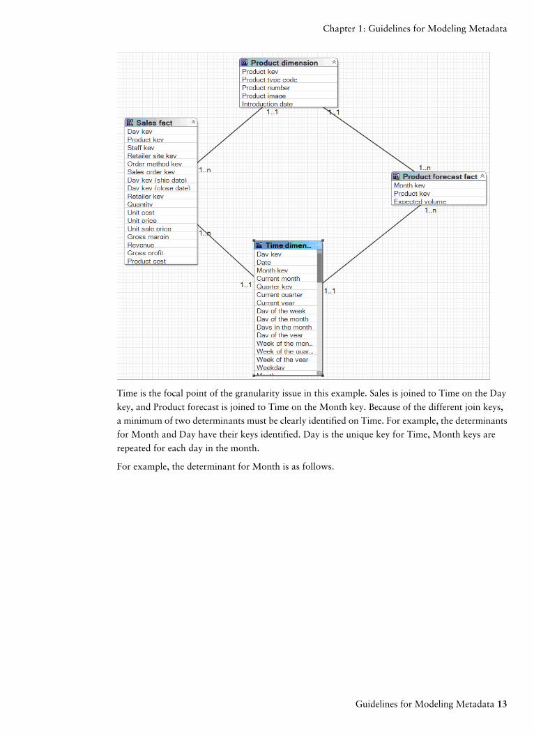
Time is the focal point of the granularity issue in this example. Sales is joined to Time on the Day

key, and Product forecast is joined to Time on the Month key. Because of the different join keys,

a minimum of two determinants must be clearly identified on Time. For example, the determinants

for Month and Day have their keys identified. Day is the unique key for Time, Month keys are

repeated for each day in the month.

For example, the determinant for Month is as follows.



The Product query subject could have at least three determinants: Product line, Product type, and

Product. It has relationships to both fact tables on the Product key. There are no granularity issues

with respect to the Product query subject.

By default, a report is aggregated to retrieve records from each fact table at the lowest common

level of granularity. If you create a report that uses Quantity from Sales, Expected volume from

Product forecast, Month from Time, and Product name from Product, the report retrieves records

from each fact table at the lowest common level of granularity. In this example, it is at the month

and product level.

To prevent double-counting when data exists at multiple levels of granularity, create at least two

determinants for the Time query subject. For an example, see "Determinants" (p. 8).

Expected volumeQuantityProduct nameMonth

1,6901,410Aloe ReliefApril 2007

125132Course Pro UmbrellaApril 2007

245270Aloe ReliefFebruary 2007

1Course Pro UmbrellaFebruary 2007

9288Aloe ReliefFebruary 2006

If you do not specify the determinants properly in the Time query subject, incorrect aggregation

may occur. For example, Expected volume values that exist at the Month level in Product forecast

is repeated for each day in the Time query subject. If determinants are not set correctly, the values

for Expected volume are multiplied by the number of days in the month.



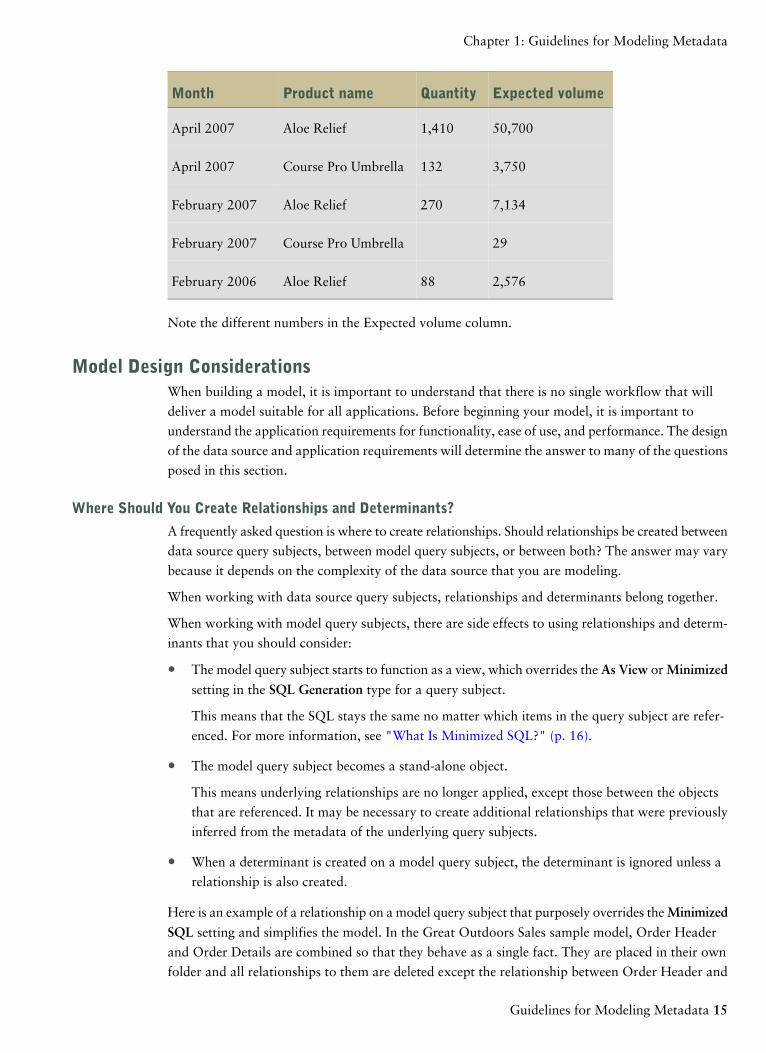
Expected volumeQuantityProduct nameMonth

50,7001,410Aloe ReliefApril 2007

3,750132Course Pro UmbrellaApril 2007

7,134270Aloe ReliefFebruary 2007

29Course Pro UmbrellaFebruary 2007

2,57688Aloe ReliefFebruary 2006

Note the different numbers in the Expected volume column.

Model Design ConsiderationsWhen building a model, it is important to understand that there is no single workflow that will

deliver a model suitable for all applications. Before beginning your model, it is important to

understand the application requirements for functionality, ease of use, and performance. The design

of the data source and application requirements will determine the answer to many of the questions

posed in this section.

Where Should You Create Relationships and Determinants?

A frequently asked question is where to create relationships. Should relationships be created between

data source query subjects, between model query subjects, or between both? The answer may vary

because it depends on the complexity of the data source that you are modeling.

When working with data source query subjects, relationships and determinants belong together.

When working with model query subjects, there are side effects to using relationships and determ-

inants that you should consider:

● The model query subject starts to function as a view, which overrides the As View or Minimized

setting in the SQL Generation type for a query subject.

This means that the SQL stays the same no matter which items in the query subject are refer-

enced. For more information, see "What Is Minimized SQL?" (p. 16).

● The model query subject becomes a stand-alone object.

This means underlying relationships are no longer applied, except those between the objects

that are referenced. It may be necessary to create additional relationships that were previously

inferred from the metadata of the underlying query subjects.

● When a determinant is created on a model query subject, the determinant is ignored unless a

relationship is also created.

Here is an example of a relationship on a model query subject that purposely overrides theMinimized

SQL setting and simplifies the model. In the Great Outdoors Sales sample model, Order Header

and Order Details are combined so that they behave as a single fact. They are placed in their own

folder and all relationships to them are deleted except the relationship between Order Header and



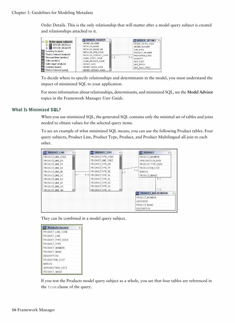
Order Details. This is the only relationship that will matter after a model query subject is created

and relationships attached to it.

To decide where to specify relationships and determinants in the model, you must understand the

impact of minimized SQL to your application.

For more information about relationships, determinants, and minimized SQL, see theModel Advisortopics in the Framework Manager User Guide.

What Is Minimized SQL?

When you use minimized SQL, the generated SQL contains only the minimal set of tables and joins

needed to obtain values for the selected query items.

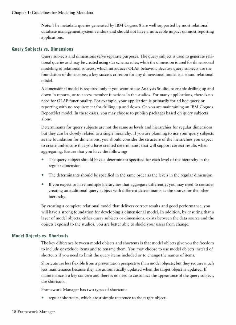
To see an example of what minimized SQL means, you can use the following Product tables. Four

query subjects, Product Line, Product Type, Product, and Product Multilingual all join to each

other.

They can be combined in a model query subject.

If you test the Products model query subject as a whole, you see that four tables are referenced in

the from clause of the query.



If you test only Product name, you see that the resulting query uses only Product Multilingual,

which is the table that was required. This is the effect of minimized SQL.

Example: When Minimized SQL Is Important

If you are modeling a normalized data source, you may be more concerned about minimized SQL

because it will reduce the number of tables used in some requests and perform better. In this case,

it would be best to create relationships and determinants between the data source query subjects

and then create model query subjects that do not have relationships.

There is a common misconception that if you do not have relationships between objects, you cannot

create star schema groups. This is not the case. Select the model query subjects to include in the

group and use the Star Schema Grouping wizard. Or you can create shortcuts and move them to a

new namespace. There is no need to have shortcuts to the relationships; this feature is purely visual

in the diagram. The effect on query generation and presentation in the studios is the same.

Example: When Minimized SQL Is Not as Important as Predictable Queries

There may be some elements in a data source that you need to encapsulate to ensure that they

behave as if they were one data object. An example might be a security table that must always be

joined to a fact. In the Great Outdoors Sales model, Order Header and Order Details are a set of

tables that together represent a fact and you would always want them to be queried together. For

an example, see "Where Should You Create Relationships and Determinants?" (p. 15).

What Is Metadata Caching?

Framework Manager stores the metadata that is imported from the data source. However depending

on governor settings and certain actions you take in the model, this metadata might not be used

when preparing a query. If you enable the Allow enhanced model portability at run time governor,

Framework Manager always queries the data source for information about the metadata before

preparing a query. If you have not enabled this governor, in most cases Framework Manager accesses

the metadata that has been stored in the model instead of querying the data source. The main

exceptions are:

● The SQL in a data source query subject has been modified. This includes the use of macros.

● A calculation or filter has been added to a data source query subject.



Note: The metadata queries generated by IBM Cognos 8 are well supported by most relational

database management system vendors and should not have a noticeable impact on most reporting

applications.

Query Subjects vs. Dimensions

Query subjects and dimensions serve separate purposes. The query subject is used to generate rela-

tional queries and may be created using star schema rules, while the dimension is used for dimensional

modeling of relational sources, which introduces OLAP behavior. Because query subjects are the

foundation of dimensions, a key success criterion for any dimensional model is a sound relational

model.

A dimensional model is required only if you want to use Analysis Studio, to enable drilling up and

down in reports, or to access member functions in the studios. For many applications, there is no

need for OLAP functionality. For example, your application is primarily for ad hoc query or

reporting with no requirement for drilling up and down. Or you are maintaining an IBM Cognos

ReportNet model. In these cases, you may choose to publish packages based on query subjects

alone.

Determinants for query subjects are not the same as levels and hierarchies for regular dimensions

but they can be closely related to a single hierarchy. If you are planning to use your query subjects

as the foundation for dimensions, you should consider the structure of the hierarchies you expect

to create and ensure that you have created determinants that will support correct results when

aggregating. Ensure that you have the following:

● The query subject should have a determinant specified for each level of the hierarchy in the

regular dimension.

● The determinants should be specified in the same order as the levels in the regular dimension.

● If you expect to have multiple hierarchies that aggregate differently, you may need to consider

creating an additional query subject with different determinants as the source for the other

hierarchy.

By creating a complete relational model that delivers correct results and good performance, you

will have a strong foundation for developing a dimensional model. In addition, by ensuring that a

layer of model objects, either query subjects or dimensions, exists between the data source and the

objects exposed to the studios, you are better able to shield your users from change.

Model Objects vs. Shortcuts

The key difference between model objects and shortcuts is that model objects give you the freedom

to include or exclude items and to rename them. You may choose to use model objects instead of

shortcuts if you need to limit the query items included or to change the names of items.

Shortcuts are less flexible from a presentation perspective than model objects, but they require much

less maintenance because they are automatically updated when the target object is updated. If

maintenance is a key concern and there is no need to customize the appearance of the query subject,

use shortcuts.

Framework Manager has two types of shortcuts:

● regular shortcuts, which are a simple reference to the target object.



● alias shortcuts, which behave as if they were a copy of the original object with completely

independent behavior. Alias shortcuts are available only for query subjects and dimensions.

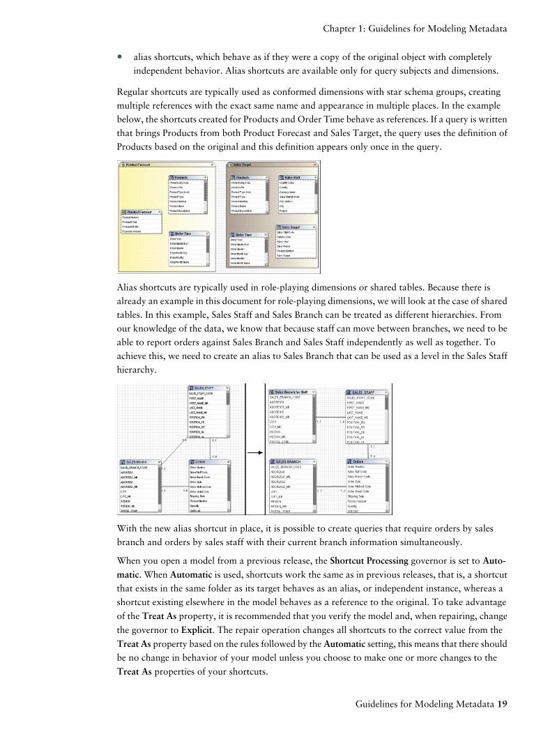
Regular shortcuts are typically used as conformed dimensions with star schema groups, creating

multiple references with the exact same name and appearance in multiple places. In the example

below, the shortcuts created for Products and Order Time behave as references. If a query is written

that brings Products from both Product Forecast and Sales Target, the query uses the definition of

Products based on the original and this definition appears only once in the query.

Alias shortcuts are typically used in role-playing dimensions or shared tables. Because there is

already an example in this document for role-playing dimensions, we will look at the case of shared

tables. In this example, Sales Staff and Sales Branch can be treated as different hierarchies. From

our knowledge of the data, we know that because staff can move between branches, we need to be

able to report orders against Sales Branch and Sales Staff independently as well as together. To

achieve this, we need to create an alias to Sales Branch that can be used as a level in the Sales Staff

hierarchy.

With the new alias shortcut in place, it is possible to create queries that require orders by sales

branch and orders by sales staff with their current branch information simultaneously.

When you open a model from a previous release, the Shortcut Processing governor is set to Auto-

matic. When Automatic is used, shortcuts work the same as in previous releases, that is, a shortcut

that exists in the same folder as its target behaves as an alias, or independent instance, whereas a

shortcut existing elsewhere in the model behaves as a reference to the original. To take advantage

of the Treat As property, it is recommended that you verify the model and, when repairing, change

the governor to Explicit. The repair operation changes all shortcuts to the correct value from the

Treat As property based on the rules followed by the Automatic setting, this means that there should

be no change in behavior of your model unless you choose to make one or more changes to the

Treat As properties of your shortcuts.



When you create a new model, the Shortcut Processing governor is always set to Explicit.

When the governor is set to Explicit, the shortcut behavior is taken from the Treat As property and

you have complete control over how shortcuts behave without being concerned about where in the

model they are located.

Folders vs. Namespaces

The most important thing to know about namespaces is that once you have begun authoring reports,

any changes you make to the names of published namespaces will impact your IBM Cognos 8

content. This is because changing the name of the namespace changes the IDs of the objects published

in the metadata. Because the namespace is used as part of the object ID in IBM Cognos 8, each

namespace must have a unique name in the model. Each object in a namespace must also have a

unique name. Part of the strategy of star schema groups is placing shortcuts into a separate

namespace, which automatically creates a unique ID for each object in the namespace. This allows

us to use the same name for shortcuts to conformed dimensions in different star schema groups.

The next time you try to run a query, report, or analysis against the updated model, you get an

error. If you need to rename the namespace that you have published, use Analyze Publish Impactto determine which reports are impacted.

Folders are much simpler than namespaces. They are purely for organizational purposes and do

not impact object IDs or your IBM Cognos 8 content. You can create folders to organize objects

by subject or functional area. This makes it easier for you to locate metadata, particularly in large

projects.

The main drawback of folders is that they require unique names for all query subjects, dimensions,

and shortcuts. Therefore, they are not ideal for containing shared objects such as conformed

dimensions.

Setting the Order of Operations for Model Calculations

In some cases, usually for ratio-related calculations, it is useful to perform the aggregation on the

calculation terms prior to the mathematical operation.

For example, the following Order details fact contains information about each order:

Margin is a calculation that computes the ratio of profit:

Margin = (Revenue - Product cost) / Revenue

If we run a query to show Revenue, Product cost, and Margin for each product using the Order

details fact, we get the following results:



MarginProduct costRevenueProduct number

61038%$11,292,005$23,057,1411

49606%$6,607,904$11,333,5182

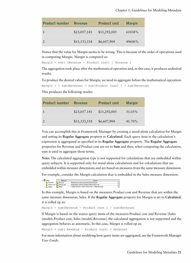
Notice that the value for Margin seems to be wrong. This is because of the order of operations used

in computing Margin. Margin is computed as:

Margin = sum( (Revenue - Product cost) / Revenue )

The aggregation took place after the mathematical operation and, in this case, it produces undesired

results.

To produce the desired values for Margin, we need to aggregate before the mathematical operation:

Margin = ( sum(Revenue) - sum(Product cost) ) / sum(Revenue)

This produces the following results:

MarginProduct costRevenueProduct number

51.03%$11,292,005$23,057.1411

41.70%$6,607,904$11,333,5182

You can accomplish this in Framework Manager by creating a stand-alone calculation for Margin

and setting its Regular Aggregate property to Calculated. Each query item in the calculation's

expression is aggregated as specified in its Regular Aggregate property. The Regular Aggregate

properties for Revenue and Product cost are set to Sum and thus, when computing the calculation,

sum is used to aggregate those terms.

Note: The calculated aggregation type is not supported for calculations that are embedded within

query subjects. It is supported only for stand-alone calculations and for calculations that are

embedded within measure dimensions and are based on measures from the same measure dimension.

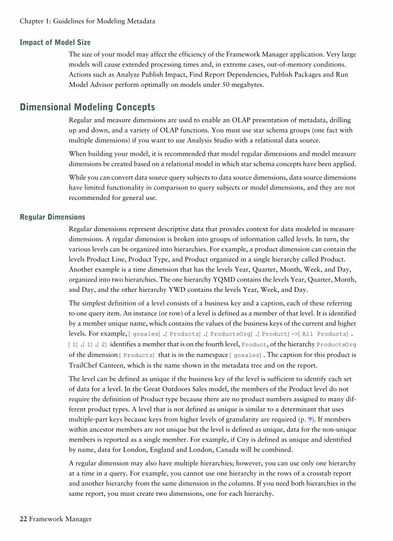
For example, consider the Margin calculation that is embedded in the Sales measure dimension:

In this example, Margin is based on the measures Product cost and Revenue that are within the

same measure dimension, Sales. If the Regular Aggregate property for Margin is set to Calculated,

it is rolled up as:

Margin = sum(Revenue - Product cost ) / sum(Revenue)

If Margin is based on the source query items of the measures Product cost and Revenue (Sales

(model).Product cost, Sales (model).Revenue), the calculated aggregation is not supported and the

aggregation behaves as automatic. In this case, Margin is rolled up as:

Margin = sum( Revenue - Product cost) / Revenue)

For more information about modifying how query items are aggregated, see the Framework Manager

User Guide.



Impact of Model Size

The size of your model may affect the efficiency of the Framework Manager application. Very large

models will cause extended processing times and, in extreme cases, out-of-memory conditions.

Actions such as Analyze Publish Impact, Find Report Dependencies, Publish Packages and Run

Model Advisor perform optimally on models under 50 megabytes.

Dimensional Modeling ConceptsRegular and measure dimensions are used to enable an OLAP presentation of metadata, drilling

up and down, and a variety of OLAP functions. You must use star schema groups (one fact with

multiple dimensions) if you want to use Analysis Studio with a relational data source.

When building your model, it is recommended that model regular dimensions and model measure

dimensions be created based on a relational model in which star schema concepts have been applied.

While you can convert data source query subjects to data source dimensions, data source dimensions

have limited functionality in comparison to query subjects or model dimensions, and they are not

recommended for general use.

Regular Dimensions

Regular dimensions represent descriptive data that provides context for data modeled in measure

dimensions. A regular dimension is broken into groups of information called levels. In turn, the

various levels can be organized into hierarchies. For example, a product dimension can contain the

levels Product Line, Product Type, and Product organized in a single hierarchy called Product.

Another example is a time dimension that has the levels Year, Quarter, Month, Week, and Day,

organized into two hierarchies. The one hierarchy YQMD contains the levels Year, Quarter, Month,

and Day, and the other hierarchy YWD contains the levels Year, Week, and Day.

The simplest definition of a level consists of a business key and a caption, each of these referring

to one query item. An instance (or row) of a level is defined as a member of that level. It is identified

by a member unique name, which contains the values of the business keys of the current and higher

levels. For example, [gosales].[Products].[ProductsOrg].[Product]->[All Products].

[1].[1].[2] identifies a member that is on the fourth level, Product, of the hierarchy ProductsOrg

of the dimension [Products] that is in the namespace [gosales]. The caption for this product is

TrailChef Canteen, which is the name shown in the metadata tree and on the report.

The level can be defined as unique if the business key of the level is sufficient to identify each set

of data for a level. In the Great Outdoors Sales model, the members of the Product level do not

require the definition of Product type because there are no product numbers assigned to many dif-

ferent product types. A level that is not defined as unique is similar to a determinant that uses

multiple-part keys because keys from higher levels of granularity are required (p. 9). If members

within ancestor members are not unique but the level is defined as unique, data for the non-unique

members is reported as a single member. For example, if City is defined as unique and identified

by name, data for London, England and London, Canada will be combined.

A regular dimension may also have multiple hierarchies; however, you can use only one hierarchy

at a time in a query. For example, you cannot use one hierarchy in the rows of a crosstab report

and another hierarchy from the same dimension in the columns. If you need both hierarchies in the

same report, you must create two dimensions, one for each hierarchy.



Measure Dimensions

Measure dimensions represent the quantitative data described by regular dimensions. Known by

many terms in various OLAP products, a measure dimension is simply the object that contains the

fact data. Measure dimensions differ from fact query subjects because they do not include the foreign

keys used to join a fact query subject to a dimensional query subject. This is because the measure

dimension is not meant to be joined as if it were a relational data object. For query generation

purposes, a measure dimension derives its relationship to a regular dimension through the underlying

query subjects. Similarly the relationship to other measure dimensions is through regular dimensions

that are based on query subjects built to behave as conformed dimensions. To enable multiple-fact,

multiple-grain querying, you must have query subjects and determinants created appropriately

before you build regular dimensions and measure dimensions.

Scope Relationships

Scope relationships exist only between measure dimensions and regular dimensions to define the

level at which the measures are available for reporting. They are not the same as joins and do not

impact the Where clause. There are no conditions or criteria set in a scope relationship to govern

how a query is formed, it specifies only if a dimension can be queried with a specified fact. The

absence of a scope relationship may result in an error at runtime or cause fact data to be rolled up

at a high level than expected given the other items in the report.

If you set the scope relationship for the measure dimension, the same settings apply to all measures

in the measure dimension. If data is reported at a different level for the measures in the measure

dimension, you can set scope on a measure. You can specify the lowest level that the data can be

reported on.

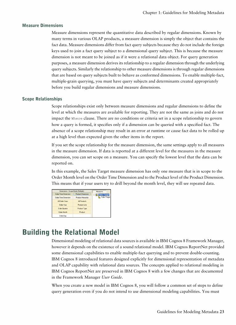
In this example, the Sales Target measure dimension has only one measure that is in scope to the

Order Month level on the Order Time Dimension and to the Product level of the Product Dimension.

This means that if your users try to drill beyond the month level, they will see repeated data.

Building the Relational ModelDimensional modeling of relational data sources is available in IBM Cognos 8 Framework Manager,

however it depends on the existence of a sound relational model. IBM Cognos ReportNet provided

some dimensional capabilities to enable multiple-fact querying and to prevent double-counting.

IBM Cognos 8 introduced features designed explicitly for dimensional representation of metadata

and OLAP capability with relational data sources. The concepts applied to relational modeling in

IBM Cognos ReportNet are preserved in IBM Cognos 8 with a few changes that are documented

in the Framework Manager User Guide.

When you create a new model in IBM Cognos 8, you will follow a common set of steps to define

query generation even if you do not intend to use dimensional modeling capabilities. You must



dimensionally model a relational data source when you want to use it in Analysis Studio, to enable

drilling up and down in reports, or to access member functions in the studios.

When you build the relational model, we recommend that you do the following:

❑ Define the relational modeling foundation (p. 24).

❑ Define the dimensional representation of the model (p. 30), if it is required.

❑ Organize the model (p. 33).

Defining the Relational Modeling FoundationA model is the set of related objects required for one or more related reporting applications. A

sound relational model is the foundation for a dimensional model.

We recommend that you do the following when you define the relational modeling foundation:

❑ Import the metadata. For information about importing, see the Framework Manager User

Guide.

❑ Verify the imported metadata (p. 24).

❑ Resolve ambiguous relationships (p. 25).

❑ Simplify the relational model using star schema concepts by analyzing cardinality for facts and

dimensions and by deciding where to put relationships and determinants (p. 15).

❑ Add data security, if required. For information about data security, see the Framework Manager

User Guide.

Then you can define the dimensional representation of the model (p. 30) if it is required, and

organize the model for presentation (p. 33).

Verifying Imported Metadata

After importing metadata, you must check the imported metadata in these areas:

● relationships and cardinality

● determinants

● the Usage property for query items

● the Regular Aggregate property for query items

Relationships and cardinality are discussed here. For information on the Usage and Regular

Aggregate properties, see the Framework Manager User Guide.

Analyzing the Cardinality for Facts and Dimensions

The cardinality of a relationship defines the number of rows of one table that is related to the rows

of another table based on a particular set (or join) of keys. Cardinality is used by IBM Cognos 8

to infer which query subjects behave as facts or dimensions. The result is that IBM Cognos 8 can

automatically resolve a common form of loop join that is caused by star schema data when you

have multiple fact tables joined to a common set of dimension tables.



To ensure predictable queries, it is important to understand how cardinality is used and to correctly

apply it in your model. It is recommended that you examine the underlying data source schema

and address areas where cardinality incorrectly identifies facts or dimensions that could cause

unpredictable query results. The Model Advisor feature in Framework Manager can be used to

help you understand how IBM Cognos 8 will interpret the cardinality you have set.

For more information, see "Cardinality" (p. 6).

Resolving Ambiguous Relationships

Ambiguous relationships occur when the data represented by a query subject or dimension can be

viewed in more than one context or role, or can be joined in more than one way. The most common

ambiguous relationships are:

● role-playing dimensions (p. 25)

● loop joins (p. 27)

● reflexive and recursive relationships (p. 28)

You can use the Model Advisor to highlight relationships that may cause issues for query generation

and resolve them in one of the ways described below. Note that there are other ways to resolve

issues than the ones discussed here. The main goal is to enable clear query paths.

Role-Playing Dimensions

A table with multiple valid relationships between itself and another table is known as a role-playing

dimension. This is most commonly seen in dimensions such as Time and Customer.

For example, the Sales fact has multiple relationships to the Time query subject on the keys Order

Day, Ship Day, and Close Day.

Remove the relationships for the imported objects, fact query subjects, and role-playing dimensional

query subjects. Create a model query subject for each role. Consider excluding unneeded query

items to reduce the length of the metadata tree displayed to your users. Ensure that a single appro-

priate relationship exists between each model query subject and the fact query subject. Note: This

will override the Minimized SQL setting but given a single table representation of the Time

dimension, it is not considered to be problematic in this case.



Decide how to use these roles with other facts that do not share the same concepts. For example,

Product forecast fact has only one time key. You need to know your data and business to determine

if all or any of the roles created for Time are applicable to Product forecast fact.

In this example, you can do one of the following:

● Create an additional query subject to be the conformed time dimension and name it clearly as

a conformed dimension.

Pick the most common role that you will use. You can then ensure that this version is joined

to all facts requiring it. In this example, Close Day has been chosen.

● You can treat Ship Day, Order Day, and Close Day as interchangeable time query subjects with

Product forecast fact.

In this case, you must create joins between each of the role-playing dimensions and Product

forecast fact. You can use only one time dimension at a time when querying the Product forecast



fact or your report may contain no data. For example, Month_key=Ship Month Key (200401)

and Month key=Close Month Key (200312).

If modeling dimensionally, use each model query subject as the source for a regular dimension, and

name the dimension and hierarchies appropriately. Ensure that there is a corresponding scope

relationship specific to each role.

Loop Joins

Loop joins in the model are typically a source of unpredictable behavior. This does not include star

schema loop joins.

Note: When cardinality clearly identifies facts and dimensions, IBM Cognos 8 can automatically

resolve loop joins that are caused by star schema data when you have multiple fact tables joined to

a common set of dimension tables.

In the case of loop joins, ambiguously defined query subjects are the primary sign of problems.

When query subjects are ambiguously defined and are part of a loop join, the joins used in a given

query are decided based on a number of factors, such as the location of relationships, the number

of segments in join paths, and, if all else is equal, the alphabetically first join path. This creates

confusion for your users and we recommend that you model to clearly identify the join paths.

Sales Staff and Branch provide a good example of a loop join with ambiguously defined query

subjects.

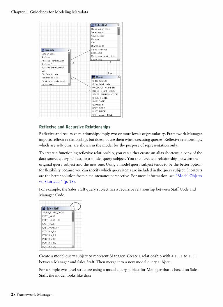
In this example, it is possible to join Branch directly to Order or through Sales Staff to Order. The

main problem is that when Branch and Order are together, you get a different result than when the

join path is Branch to Sales Staff to Order. This is because employees can move between branches

so employees who moved during the year are rolled up to their current branch even if many of the

sales they made are attributable to their previous branch. Because of the way this is modeled, there

is no guarantee which join path will be chosen and it is likely to vary depending on which items

are selected in the query.



Reflexive and Recursive Relationships

Reflexive and recursive relationships imply two or more levels of granularity. Framework Manager

imports reflexive relationships but does not use them when executing queries. Reflexive relationships,

which are self-joins, are shown in the model for the purpose of representation only.

To create a functioning reflexive relationship, you can either create an alias shortcut, a copy of the

data source query subject, or a model query subject. You then create a relationship between the

original query subject and the new one. Using a model query subject tends to be the better option

for flexibility because you can specify which query items are included in the query subject. Shortcuts

are the better solution from a maintenance perspective. For more information, see "Model Objects

vs. Shortcuts" (p. 18).

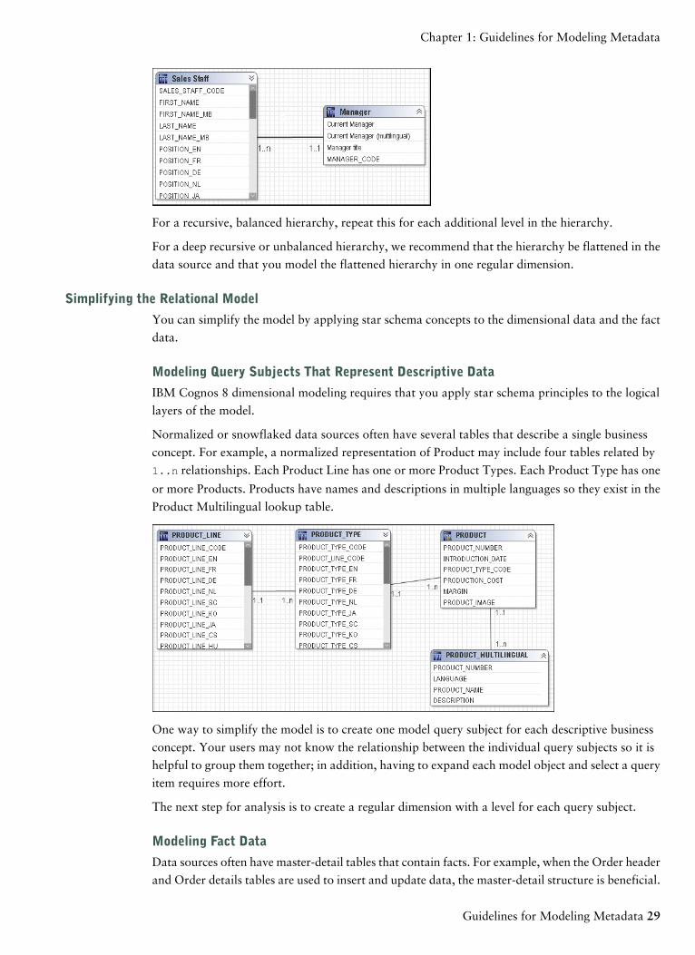
For example, the Sales Staff query subject has a recursive relationship between Staff Code and

Manager Code.

Create a model query subject to represent Manager. Create a relationship with a 1..1 to 1..n

between Manager and Sales Staff. Then merge into a new model query subject.

For a simple two-level structure using a model query subject for Manager that is based on Sales

Staff, the model looks like this:



For a recursive, balanced hierarchy, repeat this for each additional level in the hierarchy.

For a deep recursive or unbalanced hierarchy, we recommend that the hierarchy be flattened in the

data source and that you model the flattened hierarchy in one regular dimension.

Simplifying the Relational Model

You can simplify the model by applying star schema concepts to the dimensional data and the fact

data.

Modeling Query Subjects That Represent Descriptive Data

IBM Cognos 8 dimensional modeling requires that you apply star schema principles to the logical

layers of the model.

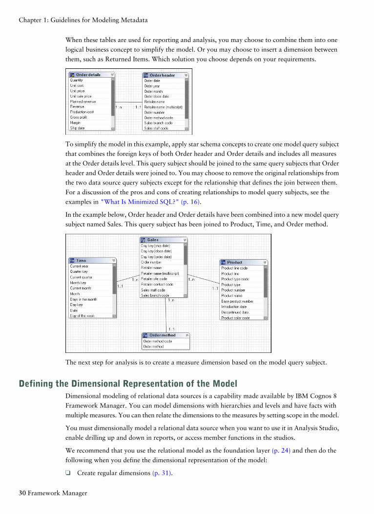
Normalized or snowflaked data sources often have several tables that describe a single business

concept. For example, a normalized representation of Product may include four tables related by

1..n relationships. Each Product Line has one or more Product Types. Each Product Type has one

or more Products. Products have names and descriptions in multiple languages so they exist in the

Product Multilingual lookup table.

One way to simplify the model is to create one model query subject for each descriptive business

concept. Your users may not know the relationship between the individual query subjects so it is

helpful to group them together; in addition, having to expand each model object and select a query

item requires more effort.

The next step for analysis is to create a regular dimension with a level for each query subject.

Modeling Fact Data

Data sources often have master-detail tables that contain facts. For example, when the Order header

and Order details tables are used to insert and update data, the master-detail structure is beneficial.



When these tables are used for reporting and analysis, you may choose to combine them into one

logical business concept to simplify the model. Or you may choose to insert a dimension between

them, such as Returned Items. Which solution you choose depends on your requirements.

To simplify the model in this example, apply star schema concepts to create one model query subject

that combines the foreign keys of both Order header and Order details and includes all measures

at the Order details level. This query subject should be joined to the same query subjects that Order

header and Order details were joined to. You may choose to remove the original relationships from

the two data source query subjects except for the relationship that defines the join between them.

For a discussion of the pros and cons of creating relationships to model query subjects, see the

examples in "What Is Minimized SQL?" (p. 16).

In the example below, Order header and Order details have been combined into a new model query

subject named Sales. This query subject has been joined to Product, Time, and Order method.

The next step for analysis is to create a measure dimension based on the model query subject.

Defining the Dimensional Representation of the ModelDimensional modeling of relational data sources is a capability made available by IBM Cognos 8

Framework Manager. You can model dimensions with hierarchies and levels and have facts with

multiple measures. You can then relate the dimensions to the measures by setting scope in the model.

You must dimensionally model a relational data source when you want to use it in Analysis Studio,

enable drilling up and down in reports, or access member functions in the studios.

We recommend that you use the relational model as the foundation layer (p. 24) and then do the

following when you define the dimensional representation of the model:

❑ Create regular dimensions (p. 31).



❑ Model dimensions with multiple hierarchies (p. 31).

❑ Create measure dimensions (p. 32).

❑ Create scope relationships (p. 33).

Then you can organize the model for presentation (p. 33).

Creating Regular Dimensions

A regular dimension contains descriptive and business key information and organizes the information

in a hierarchy, from the highest level of granularity to the lowest. It usually has multiple levels and

each level requires a key and a caption. If you do not have a single key for your level, it is recom-

mended that you create one in a calculation.

Model regular dimensions are based on data source or model query subjects that are already defined

in the model. You must define a business key and a string type caption for each level. When you

verify the model, the absence of business keys and caption information is detected. Instead of joining

model regular dimensions to measure dimensions, create joins on the underlying query subjects and

create a scope relationship between the regular dimension and the measure dimension.

Modeling Dimensions with Multiple Hierarchies

Multiple hierarchies occur when different structural views can be applied to the same data.

Depending on the nature of the hierarchies and the required reports, you may need to evaluate the

modeling technique applied to a particular case.

For example, sales staff can be viewed by manager or geography. In the IBM Cognos 8 studios,

these hierarchies are separate but interchangeable logical structures, which are bound to the same

underlying query.

Here is sales staff as a single dimension with two hierarchies:

The hierarchies are defined in Framework Manager as follows.



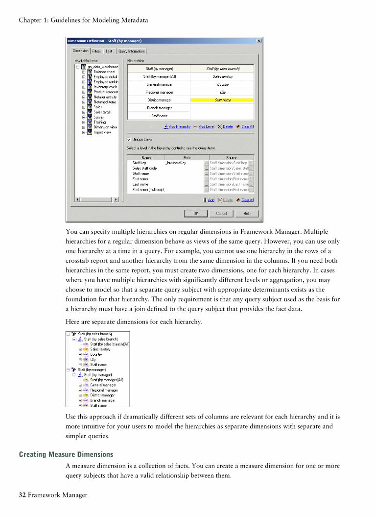
You can specify multiple hierarchies on regular dimensions in Framework Manager. Multiple

hierarchies for a regular dimension behave as views of the same query. However, you can use only

one hierarchy at a time in a query. For example, you cannot use one hierarchy in the rows of a

crosstab report and another hierarchy from the same dimension in the columns. If you need both

hierarchies in the same report, you must create two dimensions, one for each hierarchy. In cases

where you have multiple hierarchies with significantly different levels or aggregation, you may

choose to model so that a separate query subject with appropriate determinants exists as the

foundation for that hierarchy. The only requirement is that any query subject used as the basis for

a hierarchy must have a join defined to the query subject that provides the fact data.

Here are separate dimensions for each hierarchy.

Use this approach if dramatically different sets of columns are relevant for each hierarchy and it is

more intuitive for your users to model the hierarchies as separate dimensions with separate and

simpler queries.

Creating Measure Dimensions

A measure dimension is a collection of facts. You can create a measure dimension for one or more

query subjects that have a valid relationship between them.



Model measure dimensions should be composed of only quantitative items. Because, by design,

model measure dimensions do not contain keys on which to join, it is not possible to create joins

to model measure dimensions. Instead of joining model measure dimensions to regular dimensions,

create joins on the underlying query subjects. Then either manually create a scope relationship

between them or detect scope if both dimensions are in the same namespace.

Create Scope Relationships

Scope relationships exist only between measure dimensions and regular dimensions to define the

level at which the measures are available for reporting. They are not the same as joins and do not

impact the Where clause. There are no conditions or criteria set in a scope relationship to govern

how a query is formed, it specifies only if a dimension can be queried with a specified fact. The

absence of a scope relationship results in an error at runtime.

If you set the scope relationship for the measure dimension, the same settings apply to all measures

in the measure dimension. If data is reported at a different level for the measures in the measure

dimension, you can set scope on a measure. You can specify the lowest level that the data can be

reported on.

When you create a measure dimension, Framework Manager creates a scope relationship between

the measure dimension and each existing regular dimension. Framework Manager looks for a join

path between the measure dimension and the regular dimensions, starting with the lowest level of

detail. If there are many join paths available, the scope relationship that Framework Manager creates

may not be the one that you intended. In this case, you must edit the scope relationship.

Organizing the ModelAfter working in the relational modeling foundation (p. 24) and creating a dimensional represent-

ation (p. 30), we recommend that you do the following to organize the model:

❑ Keep the metadata from the data source in a separate namespace or folder.

❑ Create one or more optional namespaces or folders for resolving complexities that affect

querying using query subjects.

To use Analysis Studio, there must be a namespace or folder in the model that represents the

metadata with dimensional objects.

❑ Create one or more namespaces or folders for the augmented business view of the metadata

that contains shortcuts to dimensions or query subjects.

Use business concepts to model the business view. One model can contain many business views,

each suited to a different user group. You publish the business views.

❑ Create the star schema groups (p. 34).

❑ Apply object security, if required.

❑ Create packages and publish the metadata.

For information about the topics not covered here, see the Framework Manager User Guide.



Star Schema Groups

The concept of the conformed dimension is not isolated to dimensional modeling, it applies equally

to query subjects.

Use the Star Schema Grouping wizard to quickly create groups of shortcuts that will provide context

for your users regarding which objects belong together. This makes the model more intuitive for

your users. Star schema groups can also facilitate multiple-fact reporting by allowing the repetition

of shared dimensions in different groups. This helps your users to see what different groups have

in common and how they can do cross-functional, or multiple-fact, reporting. For more information,

see "Multiple-fact, Multiple-grain Queries" (p. 12).

Star schema groups also provide context for queries with multiple join paths. By creating star schema

groups in the business view of the model, you can clarify which join path to select when many are

available. This is particularly useful for fact-less queries.

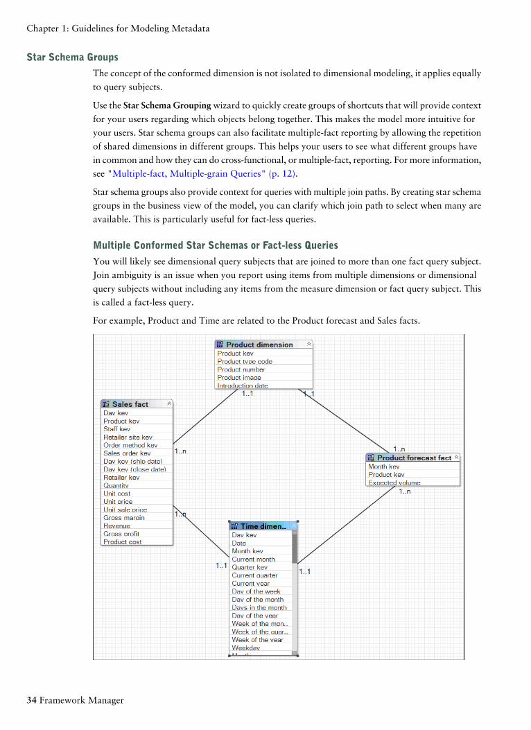
Multiple Conformed Star Schemas or Fact-less Queries

You will likely see dimensional query subjects that are joined to more than one fact query subject.

Join ambiguity is an issue when you report using items from multiple dimensions or dimensional

query subjects without including any items from the measure dimension or fact query subject. This

is called a fact-less query.

For example, Product and Time are related to the Product forecast and Sales facts.



Using these relationships, how do you write a report that uses only items from Product and Time?

The business question could be which products were forecasted for sale in 2005 or which products

were actually sold in 2005. Although this query involves only Product and Time, these dimensions

are related through multiple facts. There is no way to guess which business question is being asked.

You must set the context for the fact-less query.

In this example, we recommend that you create two namespaces, one containing shortcuts to

Product, Time, and Product forecast, and another containing Product, Time, and Sales.

When you do this for all star schemas, you resolve join ambiguity by placing shortcuts to the fact

and all dimensions in a single namespace. The shortcuts for conformed dimensions in each namespace

are identical and are references to the original object. Note: The exact same rule is applied to regular

dimensions and measure dimensions.

With a namespace for each star schema, it is now clear to your users which items to use. To create

a report on which products were actually sold in 2005, they use Product and Year from the Sales

Namespace. The only relationship that is relevant in this context is the relationship between Product,

Time, and Sales, and it is used to return the data.





Chapter 2: The SQL Generated by IBM Cognos 8

The SQL generated by IBM Cognos 8 is often misunderstood. This document explains the SQL

that results in common situations.

Note: The SQL examples shown in this document were edited for length and are used to highlight

specific examples. These examples use the version 8.2 sample model and will be updated in a sub-

sequent release.

To access this document in a different language, go to installation location\cognos\c8\webcontent\

documentation and open the folder for the language you want. Then open ug_best.pdf.

Understanding Dimensional QueriesDimensional queries are designed to enable multiple-fact querying. The basic goals of multiple-fact

querying are:

● Preserve data when fact data does not perfectly align across common dimensions, such as when

there are more rows in the facts than in the dimensions.

● Prevent double-counting when fact data exists at different levels of granularity by ensuring that

each fact is represented in a single query with appropriate grouping. Determinants may need

to be created for the underlying query subjects in some cases.

Single Fact QueryA query on a star schema group results in a single fact query.

In this example, Sales is the focus of any query written. The dimensions provide attributes and

descriptions to make the data in Sales more meaningful. All relationships between dimensions and

the fact are 1-n.


When you filter on the month and product, the result is as follows.

Multiple-fact, Multiple-grain Query on Conformed DimensionsA query on multiple facts and conformed dimensions respects the cardinality between each fact

table and its dimensions and writes SQL to return all the rows from each fact table.

For example, Sales and Product Forecast are both facts.



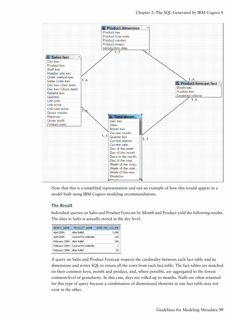
Note that this is a simplified representation and not an example of how this would appear in a

model built using IBM Cognos modeling recommendations.

The Result

Individual queries on Sales and Product Forecast by Month and Product yield the following results.

The data in Sales is actually stored at the day level.

A query on Sales and Product Forecast respects the cardinality between each fact table and its

dimensions and writes SQL to return all the rows from each fact table. The fact tables are matched

on their common keys, month and product, and, where possible, are aggregated to the lowest

common level of granularity. In this case, days are rolled up to months. Nulls are often returned

for this type of query because a combination of dimensional elements in one fact table may not

exist in the other.



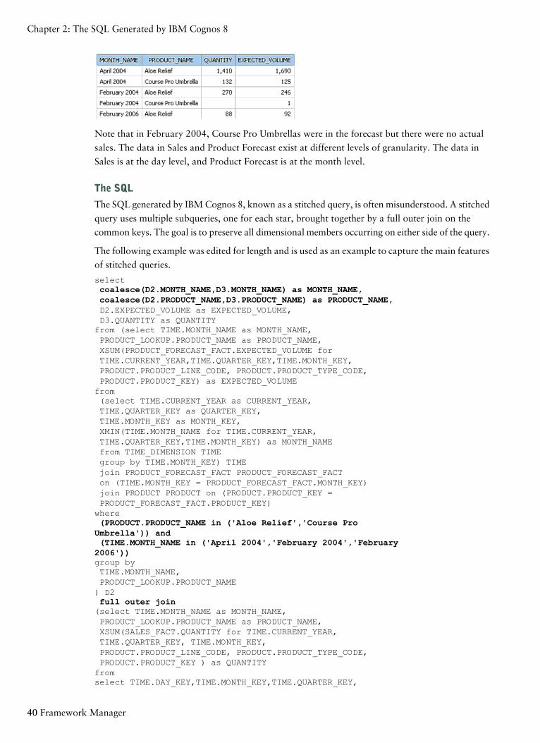
Note that in February 2004, Course Pro Umbrellas were in the forecast but there were no actual

sales. The data in Sales and Product Forecast exist at different levels of granularity. The data in

Sales is at the day level, and Product Forecast is at the month level.

The SQL

The SQL generated by IBM Cognos 8, known as a stitched query, is often misunderstood. A stitched

query uses multiple subqueries, one for each star, brought together by a full outer join on the

common keys. The goal is to preserve all dimensional members occurring on either side of the query.

The following example was edited for length and is used as an example to capture the main features

of stitched queries.

selectcoalesce(D2.MONTH_NAME,D3.MONTH_NAME) as MONTH_NAME,coalesce(D2.PRODUCT_NAME,D3.PRODUCT_NAME) as PRODUCT_NAME,D2.EXPECTED_VOLUME as EXPECTED_VOLUME,D3.QUANTITY as QUANTITYfrom (select TIME.MONTH_NAME as MONTH_NAME,PRODUCT_LOOKUP.PRODUCT_NAME as PRODUCT_NAME,XSUM(PRODUCT_FORECAST_FACT.EXPECTED_VOLUME forTIME.CURRENT_YEAR,TIME.QUARTER_KEY,TIME.MONTH_KEY,PRODUCT.PRODUCT_LINE_CODE, PRODUCT.PRODUCT_TYPE_CODE,PRODUCT.PRODUCT_KEY) as EXPECTED_VOLUMEfrom(select TIME.CURRENT_YEAR as CURRENT_YEAR,TIME.QUARTER_KEY as QUARTER_KEY,TIME.MONTH_KEY as MONTH_KEY,XMIN(TIME.MONTH_NAME for TIME.CURRENT_YEAR,TIME.QUARTER_KEY,TIME.MONTH_KEY) as MONTH_NAMEfrom TIME_DIMENSION TIMEgroup by TIME.MONTH_KEY) TIMEjoin PRODUCT_FORECAST_FACT PRODUCT_FORECAST_FACTon (TIME.MONTH_KEY = PRODUCT_FORECAST_FACT.MONTH_KEY)join PRODUCT PRODUCT on (PRODUCT.PRODUCT_KEY =PRODUCT_FORECAST_FACT.PRODUCT_KEY)where(PRODUCT.PRODUCT_NAME in ('Aloe Relief','Course ProUmbrella')) and(TIME.MONTH_NAME in ('April 2004','February 2004','February2006'))group byTIME.MONTH_NAME,PRODUCT_LOOKUP.PRODUCT_NAME) D2full outer join(select TIME.MONTH_NAME as MONTH_NAME,PRODUCT_LOOKUP.PRODUCT_NAME as PRODUCT_NAME,XSUM(SALES_FACT.QUANTITY for TIME.CURRENT_YEAR,TIME.QUARTER_KEY, TIME.MONTH_KEY,PRODUCT.PRODUCT_LINE_CODE, PRODUCT.PRODUCT_TYPE_CODE,PRODUCT.PRODUCT_KEY ) as QUANTITYfromselect TIME.DAY_KEY,TIME.MONTH_KEY,TIME.QUARTER_KEY,



TIME.CURRENT_YEAR,TIME.MONTH_EN as MONTH_NAMEfrom TIME_DIMENSION TIME) TIMEjoin SALES_FACT SALES_FACTon (TIME.DAY_KEY = SALES_FACT.ORDER_DAY_KEY)join PRODUCT PRODUCT on (PRODUCT.PRODUCT_KEY = SALES_FACT.PRODUCT_KEY)wherePRODUCT.PRODUCT_NAME in ('Aloe Relief','Course Pro Umbrella'))and (TIME.MONTH_NAME in ('April 2004','February 2004','February2006'))group byTIME.MONTH_NAME,PRODUCT.PRODUCT_NAME) D3on ((D2.MONTH_NAME = D3.MONTH_NAME) and(D2.PRODUCT_NAME = D3.PRODUCT_NAME))

What Is the Coalesce Statement?

A coalesce statement is simply an efficient means of dealing with query items from conformed

dimensions. It is used to accept the first non-null value returned from either query subject. This

statement allows a full list of keys with no repetitions when doing a full outer join.

Why Is There a Full Outer Join?

A full outer join is necessary to ensure that all the data from each fact table is retrieved. An inner

join gives results only if an item in inventory was sold. A right outer join gives all the sales where

the items were in inventory. A left outer join gives all the items in inventory that had sales. A full

outer join is the only way to learn what was in inventory and what was sold.

Modeling 1-n Relationships as 1-1 RelationshipsIf a 1-n relationship exists in the data but is modeled as a 1-1 relationship, SQL traps cannot be

avoided because the information provided by the metadata to IBM Cognos 8 is insufficient.

The most common problems that arise if 1-n relationships are modeled as 1-1 are the following:

● Double-counting for multiple-grain queries is not automatically prevented.

IBM Cognos 8 cannot detect facts and then generate a stitched query to compensate for double-

counting, which can occur when dealing with hierarchical relationships and different levels of

granularity across conformed dimensions.

● Multiple-fact queries are not automatically detected.

IBM Cognos 8 will not have sufficient information to detect a multiple-fact query. For multiple-

fact queries, an inner join is performed and the loop join is eliminated by dropping the last

evaluated join. Dropping a join is likely to lead to incorrect or unpredictable results depending

on the dimensions and facts included in the query.

If the cardinality were modified to use only 1-1 relationships between query subjects or dimensions,

the result of a query on Product Forecast and Sales with Time or Time and Product generates a

single Select statement that drops one join to prevent a circular reference.

The example below shows that the results of this query are incorrect when compared with the results

of individual queries against Sales or Product Forecast.

The results of individual queries are as follows.



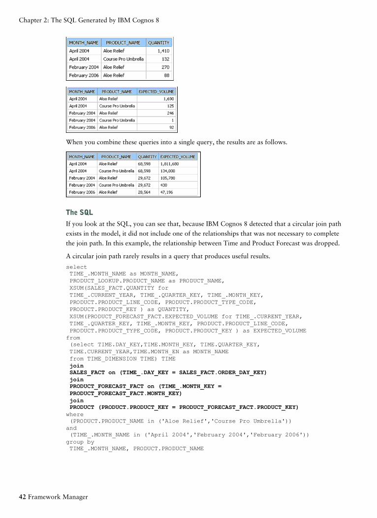
When you combine these queries into a single query, the results are as follows.

The SQL

If you look at the SQL, you can see that, because IBM Cognos 8 detected that a circular join path

exists in the model, it did not include one of the relationships that was not necessary to complete

the join path. In this example, the relationship between Time and Product Forecast was dropped.

A circular join path rarely results in a query that produces useful results.

selectTIME_.MONTH_NAME as MONTH_NAME,PRODUCT_LOOKUP.PRODUCT_NAME as PRODUCT_NAME,XSUM(SALES_FACT.QUANTITY forTIME_.CURRENT_YEAR, TIME_.QUARTER_KEY, TIME_.MONTH_KEY,PRODUCT.PRODUCT_LINE_CODE, PRODUCT.PRODUCT_TYPE_CODE,PRODUCT.PRODUCT_KEY ) as QUANTITY,XSUM(PRODUCT_FORECAST_FACT.EXPECTED_VOLUME for TIME_.CURRENT_YEAR,TIME_.QUARTER_KEY, TIME_.MONTH_KEY, PRODUCT.PRODUCT_LINE_CODE,PRODUCT.PRODUCT_TYPE_CODE, PRODUCT.PRODUCT_KEY ) as EXPECTED_VOLUMEfrom(select TIME.DAY_KEY,TIME.MONTH_KEY, TIME.QUARTER_KEY,TIME.CURRENT_YEAR,TIME.MONTH_EN as MONTH_NAMEfrom TIME_DIMENSION TIME) TIMEjoinSALES_FACT on (TIME_.DAY_KEY = SALES_FACT.ORDER_DAY_KEY)joinPRODUCT_FORECAST_FACT on (TIME_.MONTH_KEY =PRODUCT_FORECAST_FACT.MONTH_KEY)joinPRODUCT (PRODUCT.PRODUCT_KEY = PRODUCT_FORECAST_FACT.PRODUCT_KEY)where(PRODUCT.PRODUCT_NAME in ('Aloe Relief','Course Pro Umbrella'))and(TIME_.MONTH_NAME in ('April 2004','February 2004','February 2006'))group byTIME_.MONTH_NAME, PRODUCT.PRODUCT_NAME



Multiple-fact, Multiple-grain Query on Non-Conformed DimensionsIf a non-conformed dimension is added to the query, the nature of the result returned by the stitched

query is changed. It is no longer possible to aggregate records to a lowest common level of granu-

larity because one side of the query has dimensionality that is not common to the other side of the

query. The result returned is really two correlated lists.

The Result

The results of individual queries on the respective star schemas look like this.



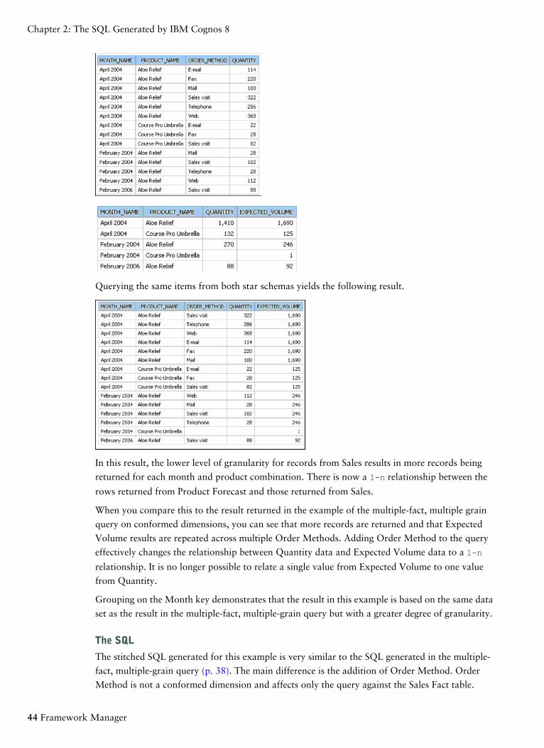
Querying the same items from both star schemas yields the following result.

In this result, the lower level of granularity for records from Sales results in more records being

returned for each month and product combination. There is now a 1-n relationship between the

rows returned from Product Forecast and those returned from Sales.

When you compare this to the result returned in the example of the multiple-fact, multiple grain

query on conformed dimensions, you can see that more records are returned and that Expected

Volume results are repeated across multiple Order Methods. Adding Order Method to the query

effectively changes the relationship between Quantity data and Expected Volume data to a 1-n

relationship. It is no longer possible to relate a single value from Expected Volume to one value

from Quantity.

Grouping on the Month key demonstrates that the result in this example is based on the same data

set as the result in the multiple-fact, multiple-grain query but with a greater degree of granularity.

The SQL

The stitched SQL generated for this example is very similar to the SQL generated in the multiple-

fact, multiple-grain query (p. 38). The main difference is the addition of Order Method. Order

Method is not a conformed dimension and affects only the query against the Sales Fact table.



selectD2.QUANTITY as QUANTITY,D3.EXPECTED_VOLUME as EXPECTED_VOLUME,coalesce(D2.PRODUCT_NAME,D3.PRODUCT_NAME) as PRODUCT_NAME,coalesce(D2.MONTH_NAME,D3.MONTH_NAME) as MONTH_NAME,D2.ORDER_METHOD as ORDER_METHODfrom(selectPRODUCT.PRODUCT_NAME as PRODUCT_NAME,TIME.MONTH_NAME as MONTH_NAME,ORDER_METHOD.ORDER_METHOD as ORDER_METHOD,XSUM(SALES_FACT.QUANTITY for TIME.CURRENT_YEAR,TIME.QUARTER_KEY,TIME.MONTH_KEY,PRODUCT.PRODUCT_LINE_CODE,PRODUCT.PRODUCT_TYPE_CODE,PRODUCT.PRODUCT_KEY,ORDER_METHOD_DIMENSION.ORDER_METHOD_KEY) asQUANTITYfromPRODUCT_DIMENSION PRODUCTjoinSALES_FACT SALES_FACTon (PRODUCT.PRODUCT_KEY = SALES_FACT.PRODUCT_KEY)joinORDER_METHOD_DIMENSION ORDER_METHODon (ORDER_METHOD.ORDER_METHOD_KEY = SALES_FACT.ORDER_METHOD_KEY)join TIME_DIMENSION TIMEon ( TIME.DAY_KEY = SALES_FACT.ORDER_DAY_KEY)where(PRODUCT.PRODUCT_NAME in ('Aloe Relief','Course Pro Umbrella'))and( TIME.MONTH_NAME in ('April 2004','February 2004','February 2006'))group byPRODUCT.PRODUCT_NAME,TIME.MONTH_NAME,ORDER_METHOD.ORDER_METHOD) D2full outer join(selectPRODUCT.PRODUCT_NAME as PRODUCT_NAME,TIME.MONTH_NAME as MONTH_NAME,XSUM(PRODUCT_FORECAST_FACT.EXPECTED_VOLUME for TIME.CURRENT_YEAR,TIME.QUARTER_KEY,TIME.MONTH_KEY,PRODUCT.PRODUCT_LINE_CODE,PRODUCT.PRODUCT_TYPE_CODE,PRODUCT.PRODUCT_KEY) as EXPECTED_VOLUMEfromPRODUCT_DIMENSION PRODUCTjoinPRODUCT_FORECAST_FACT PRODUCT_FORECAST_FACTon (PRODUCT.PRODUCT_KEY = PRODUCT_FORECAST_FACT.PRODUCT_KEY)join(selectTIME.CURRENT_YEAR as CURRENT_YEAR,TIME.QUARTER_KEY as QUARTER_KEY,TIME.MONTH_KEY as MONTH_KEY,XMIN(TIME.MONTH_NAME for TIME.CURRENT_YEAR, TIME.QUARTER_KEY,TIME.MONTH_KEY) as MONTH_NAMEfromTIME_DIMENSION TIMEgroup byTIME.CURRENT_YEAR,TIME.QUARTER_KEY,TIME.MONTH_KEY) TIMEon (TIME.MONTH_KEY = PRODUCT_FORECAST_FACT.MONTH_KEY)where(PRODUCT.PRODUCT_NAME in ('Aloe Relief','Course Pro Umbrella'))and



(TIME.MONTH_NAME in ('April 2004','February 2004','February 2006'))group byPRODUCT.PRODUCT_NAME,TIME.MONTH_NAME) D3on ((D2.PRODUCT_NAME = D3.PRODUCT_NAME) and(D2.MONTH_NAME = D3.MONTH_NAME))

Resolving Ambiguously Identified Dimensions and FactsA query subject is considered to be ambiguously defined if it participates in both n and 1 relationships

to other query subjects. An ambiguously defined query subject is not always harmful from a query

generation perspective. We suggest that you evaluate query subjects using the following cases. The

goal of this evaluation is to prevent unnecessary query splits and to ensure that any splits that do

occur are intentional and correct.

Query Subjects That Represent a Level of HierarchyOne frequent case of an ambiguously defined query subject that is not harmful is where the query

subject represents an intermediate level of a descriptive hierarchy. One example is the Product

Hierarchy found in the Great Outdoors Sales sample model.

In this example, both Product type and Product could be identified as being ambiguously defined.

However, this ambiguity is not detrimental to either the results generated or the performance of

any query using one or more of these query subjects. You do not need to fix this query pattern

because, using the rules for fact detection, only one fact is identified in any query that combines an



item from the Product forecast or Sales query subjects. It remains a best practice to collapse hier-

archies into a single regular dimension when modeling for analysis purposes.

Some queries that can be written using this example include the following:

Query subject that behaves as a fact in thequery:

Items from these query subjects are usedin a query:

Product typeProduct line and Product type

ProductProduct line, Product type, and Product

SalesProduct line, Product type, Product, and Sales

SalesProduct line and Sales

Product forecastProduct type and Product forecast

Resolving Queries That Should Not Have Been SplitIf queries are split and should not be split, you must resolve these queries.

Query subjects on the n side of all relationships are identified as facts. We can see that in the fol-

lowing example, Order Header and Country Multilingual are behaving as facts. In reality, the

Country Multilingual query subject contains only descriptive information and seems to be a lookup

table. From a dimensional or business modeling perspective, Country Multilingual is an extension

of Country.

Why is it a problem to leave the model like this?

Test this model by authoring a report on the number of orders per city, per country. Using this

model returns an incorrect result. The numbers are correct for the cities but some cities are shown

as being in the wrong country. This is an example of an incorrectly related result.



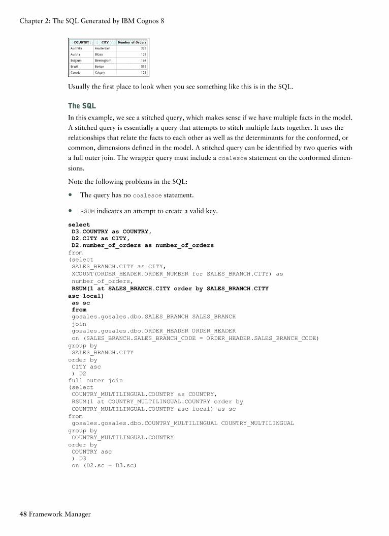
Usually the first place to look when you see something like this is in the SQL.

The SQL

In this example, we see a stitched query, which makes sense if we have multiple facts in the model.

A stitched query is essentially a query that attempts to stitch multiple facts together. It uses the

relationships that relate the facts to each other as well as the determinants for the conformed, or

common, dimensions defined in the model. A stitched query can be identified by two queries with

a full outer join. The wrapper query must include a coalesce statement on the conformed dimen-

sions.

Note the following problems in the SQL:

● The query has no coalesce statement.

● RSUM indicates an attempt to create a valid key.

selectD3.COUNTRY as COUNTRY,D2.CITY as CITY,D2.number_of_orders as number_of_ordersfrom(selectSALES_BRANCH.CITY as CITY,XCOUNT(ORDER_HEADER.ORDER_NUMBER for SALES_BRANCH.CITY) asnumber_of_orders,RSUM(1 at SALES_BRANCH.CITY order by SALES_BRANCH.CITYasc local)as scfromgosales.gosales.dbo.SALES_BRANCH SALES_BRANCHjoingosales.gosales.dbo.ORDER_HEADER ORDER_HEADERon (SALES_BRANCH.SALES_BRANCH_CODE = ORDER_HEADER.SALES_BRANCH_CODE)group bySALES_BRANCH.CITYorder byCITY asc) D2full outer join(selectCOUNTRY_MULTILINGUAL.COUNTRY as COUNTRY,RSUM(1 at COUNTRY_MULTILINGUAL.COUNTRY order byCOUNTRY_MULTILINGUAL.COUNTRY asc local) as scfromgosales.gosales.dbo.COUNTRY_MULTILINGUAL COUNTRY_MULTILINGUALgroup byCOUNTRY_MULTILINGUAL.COUNTRYorder byCOUNTRY asc) D3on (D2.sc = D3.sc)



By looking at the stitched columns in each query, we see that they are being calculated on unrelated

criteria. This explains why there is no apparent relationship between the countries and cities in the

report.

So why do we see a stitched query? To answer that question, we must look at the model.

In this example, the query items used in the report came from different query subjects. Country

came from Country Multilingual, City came from Sales Branch, and the Number of Orders came

from a count on Order Number in the Order Header query subject.

The problem is that the query splits because the query engine sees this as a multiple-fact query.

However, the split does not have a valid key on which to stitch because there is no item that both

facts have in common.

There is more than one way to solve this problem but both require understanding the data.

Solution 1

You can add a filter to Country Multilingual that changes the cardinality of the relationship to 1-1.

Select *from [GOSL].COUNTRY_MULTILINGUALWhereCOUNTRY_MULTILINGUAL."LANGUAGE"=’EN’

Or you can add a filter on the relationship and change the cardinality to 1-1.

COUNTRY.COUNTRY_CODE = COUNTRY_MULTILINGUAL.COUNTRY_CODEand COUNTRY_MULTILINGUAL.LANGUAGE = ’EN’

Either choice results in a model that has a single fact in this query.

Solution 2

Simplify the model by consolidating the related query subjects. This gives the greatest benefit by

simplifying the model and reducing the opportunities for error in query generation.



With either solution, the result of the query is now correct.

The SQL is no longer a stitched query.

selectCountry.c7 as COUNTRY,SALES_BRANCH.CITY as CITY,XCOUNT(ORDER_HEADER.ORDER_NUMBER for Country.c7,SALES_BRANCH.CITY)as number_of_ordersfrom(selectCOUNTRY.COUNTRY_CODE as c1,COUNTRY_MULTILINGUAL.COUNTRY as c7fromgosales.gosales.dbo.COUNTRY COUNTRYjoingosales.gosales.dbo.COUNTRY_MULTILINGUAL COUNTRY_MULTILINGUALon (COUNTRY.COUNTRY_CODE = COUNTRY_MULTILINGUAL.COUNTRY_CODE)where COUNTRY_MULTILINGUAL.LANGUAGE='EN') Countryjoingosales.gosales.dbo.SALES_BRANCH SALES_BRANCHon (SALES_BRANCH.COUNTRY_CODE = Country.c1)joingosales.gosales.dbo.ORDER_HEADER ORDER_HEADERon (SALES_BRANCH.SALES_BRANCH_CODE = ORDER_HEADER.SALES_BRANCH_CODE)group byCountry.c7,SALES_BRANCH.CITY



Index

Aaggregation, 8

aggregation for calculations, 20

ambiguous objects, 46

ambiguous relationships, 25

Ccalculated aggregation type, 20

calculations

order of operations, 20

cardinality

1-1, 41

1-n, 41

checking, 24

dimensions and facts, 24

queries, 6

rules, 6

types, 6

concepts, 5

conformed dimensions, 34

multiple facts, 38, 43

conformed star schema groups, 34

creating

measure dimensions, 32

regular dimensions, 31

star schema groups, 34

cross-fact queries, 24

Ddeterminants

defining, 8

query subjects, 18

dimensional data, 29

dimensionally modeling relational metadata, 30

dimensional queries, 37

multiple facts and grains, 38, 43

single fact, 37

dimensions

ambiguous, 46

hierarchies, 31

identifying, 24

measure, 22, 32

model, 12

query subjects, 12

regular, 12, 18, 22, 31

role-playing, 25

shared, 22


DMR (dimensionally modeled relational) metadata, 30

double-counting, 24, 41, 46

Ffact data, 29

fact-less query, 34

facts, 32

ambiguous, 46

identifying, 24

Ggranularity, 28

Hhierarchies, 8, 12

multiple, 31

Iimported metadata

checking, 24

Jjoins

loop, 27

Lloop joins, 24, 27

Mmaster-detail tables, 29, 32

maximum cardinality, 6

measure dimensions, 22

creating, 32


role-playing, 25

minimum cardinality, 6

model objects

shortcuts, 18

multiple-fact queries, 12, 38, 43

multiple-grain queries, 12, 38, 43

multiple hierarchies, 31

multiple valid relationships, 25, 27

Nnormalized data sources, 29

Oone-to-many relationships, 41

one-to-one relationships, 41

operations for calculations, 20

optional cardinality, 6

order of operations for calculations, 20

Qqueries

fact-less, 34

multiple-fact, 12, 38, 43

multiple-grain, 12

single fact, 37

split, 47

stitched, 24

query subjects

determinants, 18

dimensions, 12


Rrecursive relationships, 28

reflexive relationships, 28

regular dimensions, 12, 18, 22

creating, 31

hierarchies, 31

role-playing, 25

relational modeling concepts, 6

relationships

1-n, 41

ambiguous, 25

cardinality, 6

checking, 24

levels of granularity, 28

multiple valid, 25, 27

resolving

ambiguous objects, 46

split queries, 47

role-playing dimensions, 25

rules of cardinality, 6

Sshared dimensions, 22

shortcuts, 18

single fact queries, 37

snowflaked data sources, 29

split queries, 47

SQL, 37

star schema concepts, 29


creating, 34

multiple conformed, 34

stitched queries, 24

Vvalid relationships

multiple, 25


Index

Date post:	26-Aug-2018
Category:	Documents
Upload:	phungdan
View:	223 times
Download:	1 times

IBM Cognos 8 - WordPress.com · Chapter1:GuidelinesforModelingMetadata Framework Manager is a...

Documents