IC With Regime-switching

8/13/2019 IC With Regime-switching

http://slidepdf.com/reader/full/ic-with-regime-switching 1/19

a r X i v : 1 1 0 7

. 1 8 9 5 v 1

[ m a t h . O C

] 1 0 J u l 2 0 1 1

On Investment-Consumption with Regime-Switching ∗

Traian A. Pirvu

Dept of Mathematics & Statistics

McMaster University

1280 Main Street West

Hamilton, ON, L8S 4K1

[email protected]

Huayue Zhang

Dept of Finance

Nankai University

94 Weijin Road

Tianjin, China, 300071

[email protected]

July 12, 2011

Abstract. In a continuous time stochastic economy, this paper considers the problem of con-

sumption and investment in a financial market in which the representative investor exhibits a

change in the discount rate. The investment opportunities are a stock and a riskless account.

The market coefficients and discount factor switches according to a finite state Markov chain.

The change in the discount rate leads to time inconsistencies of the investor’s decisions. The

randomness in our model is driven by a Brownian motion and Markov chain. Following [3] weintroduce and characterize the equilibrium policies for power utility functions. Moreover, they

are computed in closed form for logarithmic utility function. We show that a higher discount rate

leads to a higher equilibrium consumption rate. Numerical experiments show the effect of both

time preference and risk aversion on the equilibrium policies.

Key words: Portfolio optimization, time inconsistency, equilibrium policies, regime-switching

discounting

JEL classification: G11

Mathematics Subject Classification (2000): 91B30, 60H30, 60G44

∗Work supported by NSERC grants 371653-09, 88051 and MITACS grants 5-26761, 30354 and the Natural

Science Foundation of China (10901086).

1

http://arxiv.org/abs/1107.1895v1






































1 Introduction

Dynamic asset allocation in a stochastic paradigm received a lot of scrutiny lately. The first

papers in this area are [11] and [12]. Many works then followed, most of them assuming anexponential discount rate. [3] has given an overview of the literature in the context of Merton

portfolio management problem with exponential discounting.

The issue of discounting was the subject of many studies in financial economics. Several

papers stepped away from the exponential discounting modeling, and based on empirical and

experimental evidence proposed different discount models. They can be organised in two classes:

exogenous discount rates and endogenous discount rates. In the first class the most well known

example is the hyperbolic discounting. This type discounts near future more heavily than distant

future which is in accordance with the experimental findings. [3] and [4] discuss about this class

of discounting.

The concept of endogenous time preference was developed by [8] in a discrete time formulation.

[17] considered the continuous time version which was later extended by [6]. The class of discount

rates emerged in response to the following two observed phenomena: “decreasing marginal impa-

tience” DMI and “increasing marginal impatience” IMI. DMI means that the lower the level of

consumption, the more heavily an agent discount the future. IMI is just the opposite: the higher

the level of consumption, the more heavily an agent discount the future. Some papers support

DMI, e.g. [1], others advocate for IMI, [15].

In this paper we consider a regime switching model for the financial market. This modeling is

consistent with some cyclicality observed in financial markets. Many papers considered these types

of markets for pricing derivative securities. Here we recall only two such works, [7] and [5]. In [7],

the author considers a stock price model which allows for the drift and the volatility coefficients to

switch according to two-states. This market is incomplete, but is completed with new securities.

In [5] the problem of option pricing is considered in a model where the risky underlying assets are

driven by Markov-modulated Geometric Brownian motions. A regime switching Esscher transform

is used in order to find a martingale pricing measure. When it comes to optimal investment in

regime switching markets we point to [14]. In their paper they allow for the risk preference to

switch according to the regime.

The discount rate in our paper is stochastic, exogenous and it depends on the regime. By

the best of our knowledge is the first work to consider stochastic discounting within the Mertonproblem framework. In a discrete time model, [16] considers a cyclical discount factor.

Non constant discount rates lead to time inconsistency of the decision maker as shown in [3]

and [4]. The resolution is to consider subgame perfect equilibrium strategies. These are strategies

which are optimal to implement now given that they will be implemented in the future. After we

introduce this concept we try to characterize it. In order to achieve this goal the methodology

developed in [4] is employed. That is a new result in stochastic control theory: it mixes the idea of

2



value function (from the dynamic programming principle) with the idea that in the future “optimal

trading strategies” are implemented (from the maximum principle of Pontryagin). The new twist

in our paper is the Markov chain, and the mathematical ingredient used is Ito′s formula for the

Markov-modulated diffusions. Thus, we obtain a system of four equations: first equation says

that the value function is equal to the continuation utility of subgame perfect strategies; second

equation is the wealth equation generated by subgame perfect strategies; the last two equations

relate the value function to the subgame perfect strategies. The end result is a complicated system

of PDEs, SDE and a nonlinear equation with a nonlocal term. The investor’s risk preference in

this model is of CRRA type which suggest an ansatz for the value function (it disentangles the

time, the space and the Markov chain state component). This result in subgame perfect strategies

which are time/state dependent and linear in wealth. In the special case of logarithmic utility we

can compute them explicitly. If constant discount rates, we notice that subgame perfect strategies

coincide with the optimal ones.The goal of this paper is twofold: first, to consider a model with stochastic discount rates

and second, to study the relationship between consumption and discount rates (which resembles

IMI and/or DMI ). In the Merton problem with constant discount rates we show that higher

the discount rate higher the consumption rate (this is somehow an inverse relationship to IMI).

We explore this relationship in our model with stochastic discount rates. Numerical experiments

revealed that the consumption rate is higher in the market states with higher discount rate. We

provide an analytic proof of this result for the special case of logarithmic utility. This result

is somehow consistent with the discount rate monotonocity of consumption rate in the Merton

problem. It can also explain the IMI effect: if we observe the consumption rate, then a possible

upside jump can be linked to a jump in the discount rate and vice versa. The effect of risk aversion

on the consumption rate is analysed. Here the results are consistent with [11] and [12]. That is

consumption rate is increasing in time for most levels of risk aversion except at very high levels

when is decreasing ( this can be explained by the investor’s increased appetite for risk which leads

to more investment in the risky asset and a deceasing consumption rate).

The reminder of this paper is organized as follow. In section 2 we describe the model and

formulate the objective. Section 3 contains the main result under the power utility and logarithmic

utility. In section 4, we present the numerical results. Section 5 examines consumption versus

discount rate. The paper ends with an appendix containing the proofs.

2 The Model

2.1 The Financial Market

Consider a probability space (Ω, F t0≤t≤T , F ,P), which accommodates a standard Brownian

motion W = W (t), t ≥ 0 and a homogeneous finite state continuous time Markov Chain (MC)

3



J = J (t), t ≥ 0. For simplicity assume that MC takes values in S = 0, 1. Our results hold

true in the more general situation of S having finitely many states. The filtration F t0≤t≤∞ is

the completed filtration generated by W (t)t∈[0,∞) and J (t)t∈[0,∞), that is F t = F J t F W t .

We assume that the stochastic processes W and J are independent. The MC J has a generator

Λ = [λij]S×S with λij ≥ 0 for i = j, and

j∈S λij = 0 for every i ∈ S .

In our setup the financial market consists of a bank account B and a risky asset S , that are

traded continuously over a finite time horizon [0, T ] (here T ∈ (0, ∞) is an exogenously given

deterministic time). The price process of the bank account and risky asset are governed by the

following Markov-modulated SDE:

dB(t) = r(t, J (t))B(t)dt,

dS (t) = S (t) [α(t, J (t)) dt + σ(t, J (t)) dW (t)] , 0 ≤ t ≤ ∞,

where B (0) = 1 and S (0) = s > 0 are the initial prices. The functions r(t, i), α(t, i), σ(t, i) : i ∈ S ,

are assumed to be deterministic, positive and continuous in t. Given the state i of the MC at t

they represent the riskless rate, the stock volatility and the stock return. Moreover

µ(t, i) α(t, i) − r(t, i)

stands for the stock excess return.

2.2 Investment-consumption strategies and wealth processes

In our model, a representative investor continuously invests in the stock,bond and consumes. An

acceptable investment-consumption strategy is defined below:

Definition 2.1. An R2-valued stochastic process u(t) := (π(t), c(t))t∈[0,∞) is called an admis-

sible strategy process and write u ∈ A if it is F t− progressively measurable and it satisfies the

following integrability condition

E [

t0

|π(s)µ(s, J (s)) − c(s)| ds +

t0

|π(s)σ(s, J (s))|2 ds] < ∞, a.s., for all t ∈ [0, ∞). (2.1)

Here π(t) stands for the dollar value invested in stock at time t and c(t) ≥ 0 for the consump-

tion. X u(t) := X (t) represents the wealth of the investor at time t associated with the trading

strategy u; it satisfies the following stochastic differential equation (SDE)

dX (t) = (r(t, J (t))X u(t) + µ(t, J (t))π(t) − c(t)) dt + σ(t, J (t))π(t) dW (t), (2.2)

where X (0) = x > 0 is the initial wealth and J 0 = i ∈ S is initial state. This SDE is called

the self-financing condition. Under the regularity condition (2.1) imposed on π(t), c(t)t∈[0,∞)

above, the SDE (2.2) admits a unique strong solution. In the end of this section, we introduce

further assumptions.

4





Hamilton-Jacobi-Bellman (HJB) equation

∂V

∂s

(t,s,x,i) + sup

π,c(rx + µπ − c)

∂V

∂x

(t,s,x,i) + 1

2

σ2π2 ∂ 2V

∂x2

(t,s,x,i) + U (c) (2.6)

−ρiV (t,s,x,i) + j∈S

λijV (t,s,x,j) = 0,

with the boundary condition

V (t , T , x , i) = U (x). (2.7)

Here i stands for the value of MC at time t. Thus, the HJB depends on the current time t ( through

ρi) and this dependence is inherited by the t−optimal trading strategy. This in turn leads to time

inconsistencies. The resolution is to introduce subgame perfect equilibrium strategies. They are

optimal now given that they will be implemented in the future.

3 The Main Result

3.1 The subgame perfect trading strategies

For a policy process u(t) π(t), c(t)t∈[0,T ] satisfying (2.1) and its corresponding wealth process

X (t)t∈[0,T ] given by (2.2), we denote the expected utility functional by

J (t,x,i,π,c) Ex,it

T t

e−ρi(s−t)U (c(s)) ds + e−ρi(T −t)U (X (T ))

. (3.8)

Following [3] we shall give a rigorous mathematical formulation of the equilibrium strategies in

the formal definition below.

Definition 3.1. Let F = (F 1, F 2) : [0, T ] × R+ × S → R+ × S be a map such that for any t,x > 0

and i ∈ S

lim inf ǫ↓0

J (t,x,i,F 1, F 2) − J (t,x,i,πǫ, cǫ)

ǫ ≥ 0, (3.9)

where

J (t,x,i,F 1, F 2) J (t,x,i, π, c),

π(s) F 1(s, X (s), J (s)), c(s) F 2(s, X (s), J (s)), (3.10)

and π(s), c(s)s∈[t,T ] satisfies (2.1). Here, the process X (s)s∈[t,T ] is the wealth corresponding

to π(s), c(s)s∈[t,T ]. The process πǫ(s), cǫ(s)s∈[t,T ] is another investment-consumption strategy

defined by

πǫ(s) =

π(s), s ∈ [t, T ]\E ǫ,t

π(s), s ∈ E ǫ,t,(3.11)

6



cǫ(s) =

c(s), s ∈ [t, T ]\E ǫ,t

c(s), s ∈ E ǫ,t,(3.12)

with E ǫ,t = [t, t + ǫ]; π(s), c(s)s∈E ǫ,t is any trading strategy for which πǫ(s), cǫ(s)s∈[t,T ] is an

admissible policy. If (3.9) holds true, then π(s), c(s)s∈[t,T ] is a subgame perfect strategy.

3.2 The value function

Our goal is in a first step to characterize the subgame perfect strategies and then to find them.

Inspired by [3], the value function v satisfies

v(t,x,i) = Ex,it

T

t

e−ρi(s−t)U (F 2(s, X (s), J (s))) ds + e−ρi(T −t)U ( X (T ))

. (3.13)

Recall that X (s)s∈[0,T ] is the wealth process corresponding to π(s), c(s)s∈[t,T ], so it solves the

SDE

d X (s)=[r(s, J (s)) X (s)+µ(s, J (s))F 1(s, X (s), J (s))−F 2(s, X (s), J (s))]ds+σ(s, J (s))F 1(s, X (s))dW (s).

(3.14)

Moreover, F = (F 1, F 2) is given by

F 1(t,x,i) = − µ(t, i)∂v

∂x(t,x,i)

σ2(t, i)∂ 2v

∂x2(t,x,i)

, F 2(t,x,i) = I

∂v

∂x(t,x,i)

, t ∈ [0, T ]. (3.15)

Thus, the value function is characterized by a system of four equations: one integral equationwith nonlocal term (3.13), one SDE (3.14) and two PDEs (3.15). Of course the existence of such

a function v satisfying the equations above is not a trivial issue. We will take advantage of the

special form of the utility function to simplify the problem of finding v. We search for:

v(t,x,i) = g(t, i)xγ

γ , x ≥ 0, (3.16)

where the function g(t, i) is to be found. We consider the case γ = 0 (the case of logarithmic

utility will be treated separately). In the light of equations (3.15) one gets

F 1(t,x,i) = µ(t, i)x

σ2(t, i)(1 − γ ) , F 2(t,x,i) = g

1

γ −1 (t, i)x. (3.17)

By (3.14), the associated wealth process satisfies the following SDE:

d X (s) =

r(s, J (s)) +

µ2(s, J (s))

σ2(s, J (s))(1 − γ ) − g

1γ −1 (s, J (s))

X (s)ds

+ µ(s, J (s))

σ(s, J (s))(1 − γ )X (s)dW (s). (3.18)

7



This is a linear SDE which can be easily solved. By plugging v of (3.16) into (3.13) (with

F 1, F 2 of (3.17) and X of (3.18), we obtain the following equation for g(t, i), i ∈ S :

∂g

∂t (t, i) + [γr(t, i) + µ2

(t, i

)γ

2σ2(t, i)(1 − γ ) − ρi]g(t, i) + j∈S

λijg(t, j) + (1 − γ )gγ

γ −1 (t, i) = 0, (3.19)

with the final condition g(T, i) = 1. Next we show that there exists a unique solution of this ODE

system. Let us summarize these findings:

Lemma 3.2. There exists a unique continuously differentiable solution g(t, i), i ∈ S of the system

( 3.19 ). Furthermore, v(t,x,i) = g(t, i)xγ

γ is a value function, meaning that v solves ( 3.13 ) with

F 1, F 2 of ( 3.17 ) and X of ( 3.18 ).

Appendix A proves this Lemma.

The following Theorem states the central result of our paper.

Theorem 3.3. Suppose that v(t,x,i) is given by ( 3.16 ) with g(t, i), i ∈ S the solution of the

system ( 3.19 ). Let X be the solution of SDE (3.18). Then π(t), c(t)s∈[0,T ] given by

π(t) = µ(t, J (t))X (t)

σ2(t, J (t))(1 − γ ), c(t) = g

1γ −1 (t, J (t))X (t), (3.20)

is a subgame perfect strategy.

Appendix B proves this Theorem.

Remark 3.4. In the case of constant discount rate, i.e., ρ0 = ρ1, the subgame perfect strategies

coincide with optimal ones. This can be seen by looking at the integral equation (6.34) which is

exactly HJB (2.6) (after the first order conditions are implemented).

Next we turn to the special case of logarithmic utility.

3.3 Logarithmic Utility

When the risk aversion γ

= 0, we search for the value function

v of the following form:

v(t,x,i) = h(t, i)log(x) + l(t, i). (3.21)

Arguing as in the previous subsection we find that the functions h, l : [0, T ] × S → R+ should

satisfy the following system of equations:

∂h

∂t(t, i) − ρih(t, i) +

j∈S

λijh(t, j) + 1 = 0, (3.22)

8



∂l

∂t(t, i) + (r(t, i) +

µ2(t, i)

2σ2(t, i))h(t, i) − log l(t, i) − ρil(t, i) +

j∈S

λijl(t, j) − 1 = 0,

with the final conditions h(T, i) = 1 and l(T, i) = 0. Notice that h solves a linear ODE system

and it can be found explicitly. With h known, l also solves a linear ODE system. The subgame

perfect strategy π(t), c(t)s∈[0,T ] is given by

π(t) = F 1(t, J (t))X (t)), c(t) = F 2(t, J (t))X (t)), (3.23)

with

F 1(t,x,i) = µ(t, i)x

σ2(t, i), F 2(t,x,i) = h−1(t, i)x. (3.24)

Next we want to explore the relationship between subgame perfect consumption and discount

rate. The following lemma shows that the higher discount rate the more consumption.

Lemma 3.5. Assume that ρ0 > ρ1, and h : [0, T ] × S → R+ solves the linear ODE ( 3.22 ). Then

F 2(t,x, 0) > F 2(t,x, 1) for any x > 0. In other words the subgame perfect consumption rate is

higher in the states in which the discount rate is higher.

Appendix C proves this Theorem.

4 Numerical Analysis

In this section, we use Matlab’s powerful ODE solvers (especially the functions ode23 and ode45)

to perform numerical experiments. We numerically solve ODE system (3.19) and this in turn

yield the subgame perfect strategies. Let the market coefficients be µ1 = 0.15, µ2 = 0.15, σ1 =

0.25, σ2 = 0.25, r1 = 0.05, r2 = 0.05; γ = 0.7, 0, −0.5 and −1, the discount rate ρ1 = 0.9, ρ2 =

0.3. We take the Markov Chain generator to be −6.04 6.04

10.9 −10.9

Next, define the consumption rate by

C (t, J (t)) := F 2(t, X (t), J (t))

X (t) = g

1γ −1 (t, J (t)),

with the functions g(t, i) for i = 1, 2 being the solution of (3.19).

9



0 0.5 1

0.7

0.8

0.9

1

t

γ = − 1

C(t,0)

C(t,1)

0 0.5 10.7

0.8

0.9

1

t

γ = − 0 . 5

C(t,0)

C(t,1)

0 0.5 10.7

0.8

0.9

1

t

γ = 0

C(t,0)

C(t,1)

0 0.5 10.8

1

1.2

1.4

1.6

t

γ = 0 . 7

C(t,0)

C(t,1)

Fig. 1

Fig. 1. Equilibrium proportion of wealth consumed for different γ and ρ. The x axis represents

the time, and the y axis the consumption rate C.

Remark 4.1. As t → T consumption rate approaches 1 as it was to be expected. From the picture

with γ = 0.7, we can see that the consumption rate decreases with time. This is explained by the

fact that the higher γ, the less risk aversion, which leads to higher proportion of wealth invested

into stock and less consumption. This is consistent with a graph from [11 ]. We see from the

graphs that consumption rate increases when γ increases (this is also consistent with graphs from

[ 11 ]). For a given risk aversion level γ , a higher discount rate will result in higher consumption

rate. The difference in the consumption rates in the two MC states is decreasing with respect to

γ.

5 Consumption versus Discount Rate

We were able to prove for the case of logarithmic utility that higher discount rates lead to higher

consumption rates. Numerical evidence suggest that this is also true for general power utilities.

On the other hand, in a model with constant discount rate the same result holds true as the

following Lemma shows.

10



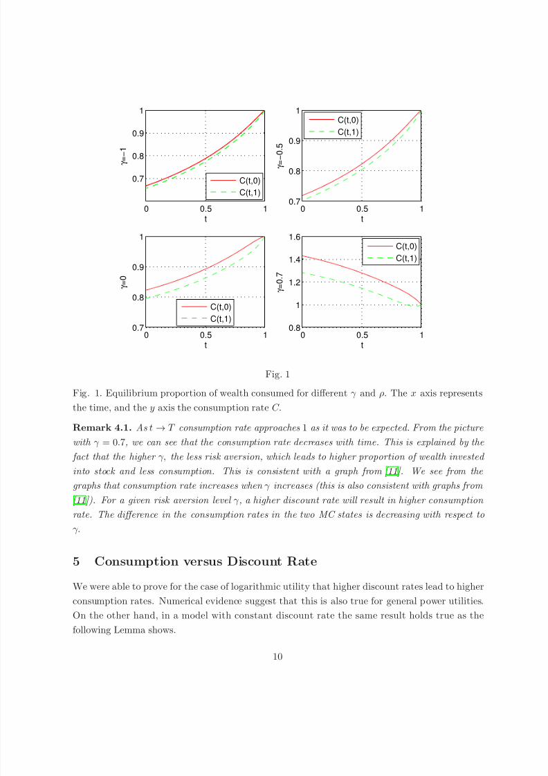
Lemma 5.1. Let C (t), t ∈ [0, T ] be the optimal consumption rate in a model with constant discount

rate ρ. Then ∂C (t)

∂ρ

> 0, t ∈ [0, T ].

Appendix D proves this Theorem.

6 Appendix

6.1 Ito’s formula for Markov Chain modulated diffusions

Suppose the stochastic processes X (t) satisfies the SDE

dX (t) = µ(t, X (t), J (t))dt + σ(t, X (t), J (t))dW (t)

X (0) = x, a.s.,

for some x ∈ R, and G(·, ·, i) ∈ C 1,3([0, T ] × R) for each i ∈ S . Then

G(t, X (t), J (t)) = G(0, x , J (0)) +

t0

ΓG(s, X (s), J (s))ds

+∂G

∂x(s, X (s), J (s))σ(s, X (s), J (s))dW (s)

+

J (t)=i

t0 (G(s, X (s), J (t)) − G(s, X (s), i))dM (t),

where

ΓG(t,x,i) = ∂G

∂t (t,x,i) + µ(t,x,i)

∂G

∂x (t,x,i) +

1

2σ2(t,x,i)

∂ 2G

∂x2 + j∈S

λij(G(t,x,j) − G(t,x,i)).

Here M (t), t ∈ [0, T ] is the martingale process associated with the Markov Chain.

6.2 A Proof of Lemma 3.2

The existence of a unique solution g of ODE system (3.19) is granted locally in time by a fixedpoint theorem. If we can establish estimates for g then this local solution is also global solution.

Let us introduce the process M (v), v t by

M (v) g(v, J v) − g(t, J t) −

vt

(gu(u, J u) + j∈S

λJ u jg(u, j))du, (6.25)

11



with g of (3.19). Dynkin formula implies that the process M (v), v t defined by (6.25) is a

martingale. Further let

K (v) exp v

t

γr(u, J (u)) + µ

2

(u, J (u))γ 2σ2(u, J (u))(1 − γ )

− ρJ (u)

du

. (6.26)

By product rule

d(K (v)g(v, J v)) = K (v)

dg(v, J v) + g(v, J v)

γr(v, J v) +

µ2(v, J v)γ

2σ2(v, J v)(1 − γ ) − ρJ v

dv

= K (v)[dM (v) + (γ − 1)gγ

γ −1 (v, J v)dv]. (6.27)

Integrating (6.27) from t to T , we get

K (T ) − g(t, J t) = T t K (v)dM (v) + (γ − 1)

T t K (v)g

γ

γ −1

(v, J v)dv. (6.28)

Taking expectation on the both sides of (6.28) and letting J t = i, it leads to

g(t, i) = EitK (T ) + (1 − γ )Ei

t

T t

K (v)gγ

γ −1 (v, J v)dv. (6.29)

Boundedness assumption on market coefficients makes the process K (v), v t of (6.27) bounded.

This in turn yields that g(t, i) is uniformly bounded from below. Next we want to prove that is

also bounded from above. For a vector y = (y1, y2,...,yn) in Rn we introduce the · 1 norm by :

y 1=

ni=1

|yi|.

When γ is positive (6.29) yields an upper bound on g (since g is bounded from below). When

γ < 0, because 0 < γ γ −1 < 1 we get from (6.29) that

g(t, 0) < E0t K (T ) + E

0t (1 − γ )

T t

K (v)g(v, J v)dv. (6.30)

g(t, 1) < E1t K (T ) + E

1t (1 − γ )

T t

K (v)g(v, J v)dv. (6.31)

Thus,

||g(t, ·)||1 ≤ 2 K + (1 − γ ) K

T t

||g(v, ·)||1dv,

for some positive constant K. Gronwal’s inequality yields an upper bound on g. Next we prove

uniqueness of the solution of (3.19). Indeed, let g1 and g2 be two solutions of (3.19), then by

12





6.3 B Proof of Theorem 3.3

We need the following Lemma which gives a PDE version of (3.13).

Lemma 6.1. For a given i ∈ S , assume there exists a function v : [0, T ] × R+ × S → R of class

C 1,2 which satisfies (3.13). Then v solves the following equation

∂v

∂t(t,x,i) + (r(t, i)x + µ(t, i)F 1(t,x,i) − F 2(t,x,i))

∂v

∂x(t,x,i) +

σ2(t, i)F 21 (t,x,i)

2

∂ 2v

∂x2(t,x,i)

+ U (F 2(t,x,i)) + j∈S

λijv(t,x,j) − ρiv(t,x,i) = 0, (6.34)

with the boundary condition v(T , x , i) = U (x).

Proof: We rewrite equation (3.13) as

v(t,x,i) =

T

t

e−ρi(s−t)f (t,s,x,i) ds + e−ρi(T −t)h(t,x,i), (6.35)

where

f (t,s,x,i) Ex,it [U (F 2(s, X (s), J (s)))], h(t,x,i) E

x,it [U ( X (T ))].

For a fixed time s, the process f (t,s, X (t), J (t))0≤t≤s is a martingale. Thus, in the light of

(3.14) the function f, h satisfy the following PDEs :

∂f

∂t (t,s,x,i) + (r(t, i)x + µ(t, i)F 1(t,x,i) − F 2(t,x,i))

∂f

∂x(t,s,x,i)

+ σ2(t, i)F 2

1

(t,x,i)

2

∂ 2f

∂x2 (t,s,x,i) + j∈S

λijf (t,x,j) = 0, f (t,t,x,i) = U (F 2(t,x,i))(6.36)

∂h

∂t (t,s,x,i) + (r(t, i)x + µ(t, i)F 1(t,x,i) − F 2(t,x,i))

∂h

∂x(t,s,x,i)

+ σ2(t, i)F 21 (t,x,i)

2

∂ 2h

∂x2(t,s,x,i) +

j∈S

λijh(t,x,j) = 0, h(T , x , i) = U (x). (6.37)

By differentiating (6.35) with respect to t we get

∂v∂t

(t,x,i) = T t

e−ρi(s−t) ∂f ∂t

(t,s,x,i) ds + e−ρi(T −t) ∂h∂t

(t,x,i) + ρiv(t,x,i) − f (t,t,x,i). (6.38)

Moreover∂v

∂x(t,x,i) =

T t

e−ρi(s−t)∂f

∂x(t,s,x,i) ds + e−ρi(T −t)

∂h

∂x(t,x,i). (6.39)

∂ 2v

∂x2(t, x) =

T t

e−ρi(s−t)∂ 2f

∂x2(t,s,x,i) ds + e−ρi(T −t)

∂ 2h

∂x2(t,x,i). (6.40)

14



In the light of (6.36), (6.37), (6.38), (6.39) and (6.40) it follows that

∂v

∂t (t,x,i) + (r(t, i)x + µ(t, i)F 1(t,x,i) − F 2(t,x,i))∂v

∂x (t,x,i) + σ2(t, i)F 2

1(t,x,i)

2

∂ 2v

∂x2 (t,x,i)

+U (F 2(t,x,i)) + j∈S

λijv(t,x,j) − ρiv(t,x,i) = 0.

Let us move to the proof of the Theorem 3.3. First let us show that

π(t) = F 1(t, J (t), X (t)) = µ(t, J (t))X (t)

σ2(t, J (t))(1 − γ ), c(t) = F 2(t, J (t)), X (t)) = g

1γ −1 (t, J (t))X (t),

(6.41)

is admissible and it satisfies (2.4) and (2.5). This claim follows easily since X of (3.18) has finite

moments of any order. Next, let us define

Γv(t,x,i) ∂v

∂t(t,x,i) +

r(t, i)x − I

∂v

∂x(t,x,i)

∂ v

∂x(t,x,i)

− µ2(t, i)

2σ2(t, i)

[∂v∂x (t,x,i)]2

∂ 2v∂x2

(t,x,i)+i∈S

λij(v(t,x,i) − v(t,x,j)) + U (c). (6.42)

Γπ,cv(t,x,i) ∂v∂t

(t,x,i) + (r(t, i)x − µ(t, i)π − c) ∂ v∂x

(t,x,i)

+ 1

2σ2(t, i)π2 ∂ 2v

∂x2(t,x,i) +

i∈S

λij(v(t,x,i) − v(t,x,j)) + U (F 2(t,x,i)).(6.43)

Then by the concavity of v and the first order conditions it follows that

Γv(t,x,i) = maxπ,c

Γπ,cv(t,x,i), (F 1(t,x,i), F 2(t,x,i)) = arg maxπ,c

Γπ,cv(t,x,i). (6.44)

Moreover, equation (6.34) can be written

Γv(t,x,i) = ρiv(t,x,i). (6.45)

Let us recall that

J (t,x,i,F 1, F 2) = v(t,x,i). (6.46)

15



Thus

J (t,x,i,F 1, F 2) − J (t,x,i,πǫ, cǫ)

= Ex,it

t+ǫ

t

e−ρi(s−t)[U (F 2(s, X (s), J (s))) − U (c(s))] ds

+ Ex,it

T t+ǫ


+ Ex,it

e−ρi(T −t)(U ( X (T )) − U (X (T )))

. (6.47)

In the light of inequalities (2.4) and (2.5) and Dominated Convergence Theorem

limǫ↓0

Ex,it

t+ǫ

t e−ρi(s−t)[U (F 2(s, X (s), J (s))) − U (c(s))] ds

ǫ

= U (F 2(t,x,i) − U (c(t)).

In the light of (6.46) it follows that

Ex,it

T t+ǫ


+ E

x,it

e−ρi(T −t)(U ( X (T )) − U (X (T )))

= E

x,it

v(t + ǫ, X (t + ǫ), J (t + ǫ)) − v(t + ǫ, X (t + ǫ), J (t + ǫ))

+ E

x,it

E[

T t+ǫ

(e−ρi(s−t) − e−ρJ (t+ε)(s−t))[U (F 2(s, X (s), J (s))) − U (F 2(s, X (s), J (s)))] ds

+ Ex,it

E[(e−ρi(T −t) − e−ρJ (t+ε)(T −t+ǫ))[U ( X (T )) − U (X (T ))]

(6.48)

In the light of inequalities (2.4), (2.5) and Dominated Convergence Theorem it follows that

limǫ↓0

Ex,it

(e−ρi(T −t) − e−ρJ (t+ε)(T −t+ǫ))[U ( X (T )) − U (X (T ))]

ε

= λij(e−ρi(T −t) − e−ρj(T −t))Ex,it

[U ( X (T )) − U (X (T ))]

= 0.

By the same token one can get that

limǫ↓0

Ex,it

T t+ǫ

(e−ρi(s−t) − e−ρJ (t+ε)(s−t))[U (F 2(s, X (s), J (s))) − U (F 2(s, X (s), J (s)))] ds

ǫ = 0.

Ito’s formula yields

Ex,it

v(t + ǫ, X (t + ǫ), J (t + ǫ)) − v(t + ǫ, X (t + ǫ), J (t + ǫ))

= E

x,it

t+ǫ

t

[Γv(s, X (s), J (s)) − U (F 2(s, X (s), J (s))]ds − Ex,it

t+ǫ

t

[Γv(s, X (s), J (s)) − U (c(s))]ds,

Therefore

16



limǫ↓0

J (t,x,i,F 1 , F 2) − J (t,x,i,πǫ, cǫ)

ǫ = [Γv(t,x,i) − Γv(t,x,i)] ≥ 0, .

the inequality follows from (6.44).

6.4 C Proof of Lemma 3.5

We know that h(t, i) solve the ODE system

∂h

∂t (t, 0) + (λ11 − ρ0)h(t, 0) + λ12h(t, 1) + 1 = 0,

∂h∂t (t, 1) + (λ22 − ρ1)h(t, 1) + λ21h(t, 0) + 1 = 0.

Let us define h(t) h(t, 0) − h(t, 1), then h satisfies the following ODE:

h′(t) + (λ11 + λ22 − ρ0)h(t) − (ρ0 − ρ1)h(t, 1) = 0

Under the assumption ρ0 > ρ1, one gets

h′(t) + (λ11 + λ22 − ρ0)h(t) > 0.

From here it follows that h(t) < 0, on [0, T ) (since h(T ) = 0). Hence, h(t, 0) < h(t, 1). Conse-

quently F

2(t,x,

0) > F

2(t,x,

1).

6.5 D Proof of Lemma 5.1

Here we are in the case of ρ0 = ρ1 = ρ. Further, for simplicity we assume constant market

coefficients α and σ. The optimal consumption rate is

C (t) = c(t)

X (t) =

η

(1 + (η − 1)eη(t−T )), (6.49)

where η ρ−γ [ (α

−

r)

2

2σ2(1−γ )+r]

1−γ . It follows from direct computations that

∂ C

∂ρ = −

1

C 2(t)[−

1

(1 − γ )η2 + eη(t−T )

1 + η(η − 1)(t − T )

η2(1 − γ ) ] (6.50)

If 1 + η(η − 1)(t − T ) ≤ 0 the claim follows. Otherwise, since

eη(T −t) > 1 + η(T − t) > 1 + η(T − t) + η2(t − T ),

17



it follows that

eη(t−T ) < 1

1 + η(η − 1)(t − T ), (6.51)

whence the result.

References

[1] Das M. (2003) Optimal growth with decreasing marginal impatience, Journal of Economic

Dynamics & Control , 27, 1881-1898.

[2] Ekeland, I. and Lazrak, A. (2010), The golden rule when preferences are time inconsis-

tent, Mathematics and Financial Economics , 4, 1-27.

[3] Ekeland, I. and Pirvu, T. A. (2008), Investment and consumption without commitment,

Mathematics and Financial Economics , 2, 57-86.

[4] Ekeland, I., Mbodji, O., and Pirvu, T. A. (2010) Time consistent portfolio manage-

ment, http://arxiv.org/pdf/1008.3407 .

[5] Elliott, R. J., Chan, L., and Siu, K., T. (2005) Option pricing and Esscher transform

under regime switching, Annals of Finance 1, 423-432.

[6] Epstein, L. G. and Hynes, J. A. (1983) The rate of time preference and dynamic economic

analysis, Journal of Political Economy , 91, 611-635

[7] Guo, X. (2001) Information and option pricing , Quantitative Finance 1, 38-44.

[8] Koopmans, T.C. (1960) Stationary utility and impatience, Econometrica 28, 287-309.

[9] Krusell, P and Smith, A. (2003) Consumption and Savings Decisions with Quasi-

geometric Discounting, Econometrica 71, 365-375.

[10] Laibson, D. (1997) Golden Eggs and Hyperbolic Discounting The Quarterly Journal of

Economics , 112, 443-477.

[11] Merton, R. C. (1969) Lifetime portfolio selection under uncertainty: the continuous-time

case, Rev. Econom. Statist. 51, 247-257.

[12] Merton, R.C. ( 1971) Optimum consumption and portfolio rules in a conitinuous-time

model. J. Economic Theory , 3, 373-413.

18

http://arxiv.org/pdf/1008.3407

http://arxiv.org/pdf/1008.3407



Date post:	03-Jun-2018
Category:	Documents
Upload:	nuno-azevedo
View:	223 times
Download:	0 times

IC With Regime-switching

Documents