September 2014 World Port Development 37 engineering numerical modelling Ice in Numerical Modelling of Sea Waves for Development of Sea Ports and Berthing Facilities – A Case Study Dr Zaman Sarker, Principal Engineer at Royal HaskoningDHV, describes a practical technique to consider sea ice in numerically transferring offshore waves into inshore for a proposed bulk terminal in a partially frozen sea environment in the Russian Far East… n recent years, there is a growing trend for development of marine berthing terminals including Liquefied Natural Gas (LNG) terminals in the frozen sea regions of the world. Reliable inshore wave conditions are important in the planning and development of such marine facilities and in making various technical and commercial decisions.Appropriate consideration of sea ice is essential in deriving such reliable inshore wave conditions.This article describes a practical technique for deriving reliable inshore wave conditions at a proposed bulk terminal considering sea ice. As part of the overall study, numerical modelling of wave transformation was carried out using the MIKE21 Spectral Wave (SW) Model of DHI (DHI, 2012) to derive inshore wave conditions at the bulk terminal. Both wind waves and swell waves were considered in association with sea ice.The methodology has been successfully applied to a project in the Russian Far East and the results presented in this paper are from this project.The methodology and lessons learnt from the study would be useful for the development of any sea port or bulk terminal in ice affected regions. At the study site the coastline is characterised by a series of headlands and bays.The sea bed contours broadly follow the alignment of the shoreline with the 5m and 10m water depth contour located approximately 100m and 250m respectively from the shoreline. The foreshore slope is of approximately 1 in 30.A dredged depth of approximately 22.0m will be maintained at the berths, in the turning circle and in the navigational approach channel. Three-hourly time-series wind and wave data for 21 years (1992 to 2012) were purchased from BMT ARGOSS (2013).The study site was located in a remote area behind islands where reliable offshore data from Global Model of BMT ARGOSS were not available. Therefore, BMT ARGOSS set up a local refined model to derive reliable offshore data for the study.The offshore wind and wave roses are shown in Figures 1 to 4.Winds blow predominantly from the north, north-westerly and south. However, most of the higher speed winds come from the north and north-westerly directions.The dominant swell wave directions are south-westerly.Dominant resultant wave directions are north, north-westerly, south and south-westerly which reflects the directions of the wind waves and swell waves.As wind waves and swell waves arrive at the site from very different directions, it was considered that a more accurate description of inshore conditions would be obtained by analysing wind waves and swell waves separately. Resultant waves were, therefore, not used in the analysis. The astronomical tidal level variation at the site is small and does not exceed 0.5m. Global sea level rise for various scenarios was extracted from the Intergovernmental Panel on Climate Change (IPCC, 2007). A sea level rise of 0.5m has been adopted for the study. Important ice terminologies have been defined as below: ☛ Sea ice coverage (also known as ice concentration) - is defined as the percentage of ice surface area over sea surface area. A 0% means no ice and 100% means total coverage by ice. ☛ Sea ice thickness - is defined as the thickness of the ice from the surface. ☛ Sea ice extent - if the ice concentration is higher than a threshold concentration e.g. 33% then the sea surface is defined as covered. ☛ Sea ice volume - is found from multiplying the concentration by the area and thickness. Sea ice shape and age - sea ice is divided into different shapes (such as frazil ice, grease ice, slush ice, shuga ice, nillas and floes) and ages (such as new ice, young ice and first year ice). ☛ Sea ice charts are used to display information about the ice in an area.The data is displayed in egg shaped blocks.This code is known as the ‘egg code’. An ice egg code consists of information on ice such as concentration, stage of development, forms and thickness. Three-hourly time-series ice data for 21 years (1992 to 2012) were purchased from BMT ARGOSS (2013). A sample time-series plot of ice coverage for 1993 is shown in Figure 5. Ice data were analysed to derive monthly and yearly averaged ice coverage (percentage) as shown in Table 1.Table 1 shows the following: ☛ Average ice conditions for each month of each year (see the body of Table 1) ☛ Monthly averaged ice condition for the entire data duration (see the right column of I Ice in Numerical Modelling of Sea Waves for Development of Sea Ports and Berthing Facilities – A Case Study Meteorological conditions Ice conditions
Transcript
September 2014 World Port Development 37
e n g i n e e r i n gn u m e r i c a l m o d e l l i n g
Ice in Numerical Modelling of Sea Waves for Developmentof Sea Ports and Berthing Facilities – A Case Study
Dr Zaman Sarker, Principal Engineer atRoyal HaskoningDHV, describes a practicaltechnique to consider sea ice in numericallytransferring offshore waves into inshorefor a proposed bulk terminal in a partiallyfrozen sea environment in the Russian FarEast…
n recent years, there is a growing trend for development of marine berthing terminals including Liquefied Natural Gas
(LNG) terminals in the frozen sea regions ofthe world. Reliable inshore wave conditions areimportant in the planning and development ofsuch marine facilities and in making varioustechnical and commercial decisions.Appropriateconsideration of sea ice is essential in derivingsuch reliable inshore wave conditions.Thisarticle describes a practical technique forderiving reliable inshore wave conditions at aproposed bulk terminal considering sea ice.As part of the overall study, numerical modelling of wave transformation was carriedout using the MIKE21 Spectral Wave (SW)Model of DHI (DHI, 2012) to derive inshorewave conditions at the bulk terminal. Bothwind waves and swell waves were consideredin association with sea ice.The methodology
has been successfully applied to a project inthe Russian Far East and the results presentedin this paper are from this project.Themethodology and lessons learnt from the studywould be useful for the development of any seaport or bulk terminal in ice affected regions.
At the study site the coastline is characterisedby a series of headlands and bays.The sea
bed contours broadly follow the alignment ofthe shoreline with the 5m and 10m waterdepth contour located approximately 100mand 250m respectively from the shoreline.The foreshore slope is of approximately 1 in30.A dredged depth of approximately 22.0mwill be maintained at the berths, in the turningcircle and in the navigational approach channel.Three-hourly time-series wind and wave datafor 21 years (1992 to 2012) were purchasedfrom BMT ARGOSS (2013).The study sitewas located in a remote area behind islandswhere reliable offshore data from GlobalModel of BMT ARGOSS were not available.Therefore, BMT ARGOSS set up a local refined model to derive reliable offshore datafor the study.The offshore wind and waveroses are shown in Figures 1 to 4.Winds blowpredominantly from the north, north-westerlyand south. However, most of the higher speedwinds come from the north and north-westerlydirections.The dominant swell wave directionsare south-westerly. Dominant resultant wave directions are north, north-westerly, south andsouth-westerly which reflects the directionsof the wind waves and swell waves.As windwaves and swell waves arrive at the site fromvery different directions, it was considered that
a more accurate description of inshore conditions would be obtained by analysing wind waves and swell waves separately. Resultantwaves were, therefore, not used in the analysis.The astronomical tidal level variation at thesite is small and does not exceed 0.5m. Globalsea level rise for various scenarios was extractedfrom the Intergovernmental Panel on ClimateChange (IPCC, 2007).A sea level rise of 0.5mhas been adopted for the study.
Important ice terminologies have beendefined as below:☛ Sea ice coverage (also known as ice concentration) - is defined as the percentageof ice surface area over sea surface area.A 0% means no ice and 100% means totalcoverage by ice.☛ Sea ice thickness - is defined as the thickness of the ice from the surface.☛ Sea ice extent - if the ice concentration ishigher than a threshold concentration e.g. 33%then the sea surface is defined as covered.☛ Sea ice volume - is found from multiplyingthe concentration by the area and thickness.Sea ice shape and age - sea ice is divided intodifferent shapes (such as frazil ice, grease ice,slush ice, shuga ice, nillas and floes) and ages (such as new ice, young ice and first year ice).☛ Sea ice charts are used to display informationabout the ice in an area.The data is displayedin egg shaped blocks.This code is known asthe ‘egg code’.An ice egg code consists ofinformation on ice such as concentration,stage of development, forms and thickness.Three-hourly time-series ice data for 21years (1992 to 2012) were purchased from
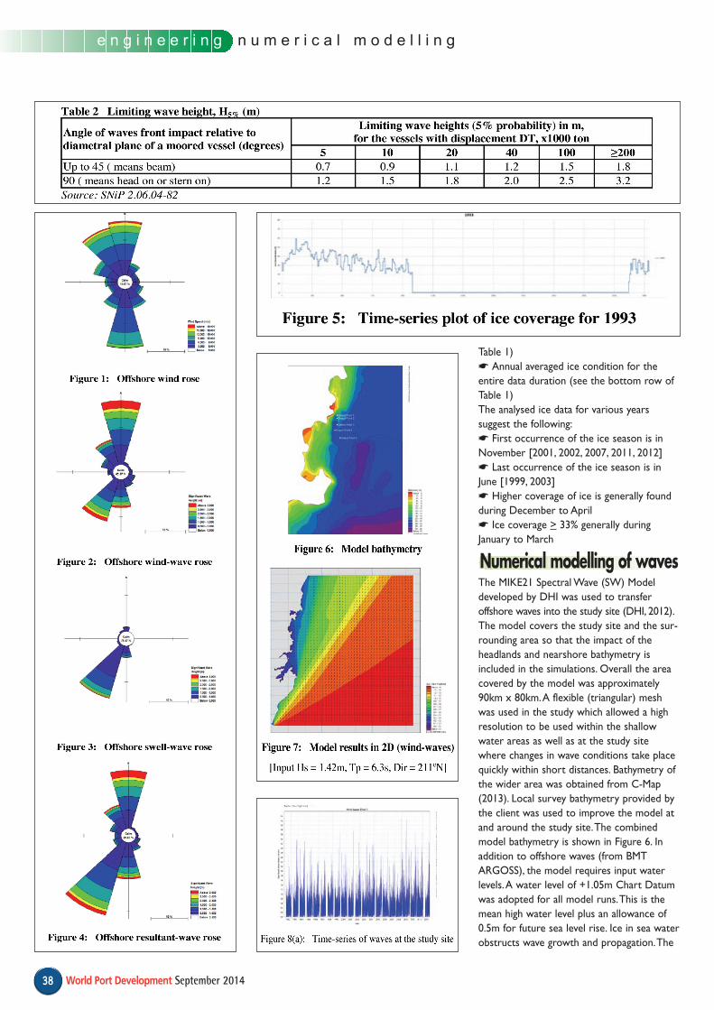
BMT ARGOSS (2013).A sample time-seriesplot of ice coverage for 1993 is shown inFigure 5. Ice data were analysed to derivemonthly and yearly averaged ice coverage(percentage) as shown in Table 1.Table 1shows the following:☛ Average ice conditions for each month ofeach year (see the body of Table 1)☛ Monthly averaged ice condition for theentire data duration (see the right column of
I
Ice in Numerical Modelling of Sea Waves for Developmentof Sea Ports and Berthing Facilities – A Case Study
Meteorological conditions
Ice conditions
World Port Development September 201438
e n g i n e e r i n g n u m e r i c a l m o d e l l i n g
Table 1)☛ Annual averaged ice condition for theentire data duration (see the bottom row ofTable 1)The analysed ice data for various years suggest the following:☛ First occurrence of the ice season is inNovember [2001, 2002, 2007, 2011, 2012]☛ Last occurrence of the ice season is inJune [1999, 2003]☛ Higher coverage of ice is generally foundduring December to April☛ Ice coverage > 33% generally duringJanuary to March
The MIKE21 Spectral Wave (SW) Modeldeveloped by DHI was used to transfer offshore waves into the study site (DHI, 2012).The model covers the study site and the sur-rounding area so that the impact of the headlands and nearshore bathymetry isincluded in the simulations. Overall the areacovered by the model was approximately90km x 80km.A flexible (triangular) meshwas used in the study which allowed a highresolution to be used within the shallowwater areas as well as at the study sitewhere changes in wave conditions take placequickly within short distances. Bathymetry ofthe wider area was obtained from C-Map(2013). Local survey bathymetry provided bythe client was used to improve the model atand around the study site.The combinedmodel bathymetry is shown in Figure 6. Inaddition to offshore waves (from BMTARGOSS), the model requires input waterlevels.A water level of +1.05m Chart Datumwas adopted for all model runs.This is themean high water level plus an allowance of0.5m for future sea level rise. Ice in sea waterobstructs wave growth and propagation.The
Numerical modelling of waves
September 2014 World Port Development 39
e n g i n e e r i n gn u m e r i c a l m o d e l l i n g
introduction of partially obstructed grid pointsin the wave model provides a more naturalway to continuously model ice coverage.Asreported in Tolman (2003), detailed analysesof the effects of ice floes on wave propagationhave been published (e.g.Wadhams et al., 1986;Masson and LeBlond, 1989; Lavrenov, 1998).It has been shown that wave attenuation inice fields shows an exponential decay inspace with a given length scale.Wave energydoes not dissipate instantaneously when thewave field encounters ice, rather waves areassumed to progressively lose energy whiletravelling through an ice field, consistent withexponential decay.The decay rates areexpected to be a distinct function of the sizeof individual ice floes (e.g. Masson and LeBond,1989), with larger ice floes scattering wavesmore efficiently and hence resulting in largerdecay rates.As the floe size increases withice concentration, decay rates increase stronglywith ice concentration. Detailed ice data arerequired to estimate such decay rates for anysophisticated approach. Due to lack of necessary ice data to estimate decay ratesrequired for the sophisticated approach, asimplified approach was used in the study.This simplified approach based on cut-off iceconcentrations was used to assess the influence of ice on wave propagation.Withinthe MIKE21 SW model the influence of ice istreated in the following way:☛ If the ice coverage (i.e. ice concentration)is greater than or equal to a threshold value(of 33%) then the model considers the icearea as land (i.e. there are no waves in theice area).☛ If the ice coverage is less than the thresholdvalue of 33% then the model considers theice area as ice-free water (i.e. there is noeffect of ice on waves).The threshold ice coverage value recommendedin the MIKE21 Manual (DHI, 2012) is alsosupported by various other studies such asTolman (2003) and Tuomi et al. (2011).Thismethod ensures that the wave model uses a
fetch starting from the ice edge. Furthermore,waves are not predicted in areas that have icecoverage greater than 33%.A 2-dimensionalice map was prepared for the study coveringthe entire model area with constant ice coverage value for a particular time step.The ice map covers the entire run duration.Months where ice coverage was > 33% wereconsidered as ice months in the model.Theseice months have been showed by green boxesin Table 1.The remainder of the months ofvarious years were considered as ice freemonths in the model. Model simulationswere carried out to transform the two typesof waves inshore as below:☛ Wind generated waves[generated locally by winds]☛ Swell waves[generated by remote meteorological conditions]Model results (wave heights and directions)were extracted for the entire modelling area(see Figure 7) as well as at selected locationswithin the navigational areas and along thejetty of the proposed dry bulk terminal (seeFigures 8-9).
The model results have been used to calculatethe operational downtime of the proposedbulk terminal. Operational (wave) downtimemay be defined as the number of days peryear when conditions at the loading andunloading berths exceed a given height andtherefore the berths will not be operational.Downtime due to adverse wave conditions forvessels at berth is an important commercialaspect in the planning and development of asea port or a berthing terminal.The wavemodel results from the study were used toassess operational downtime at the berths.Waves affecting the head and beam of a vessel(see Figure 10) were considered separatelyfor a wide range of vessel sizes.The downtimeassessment was carried out according to theRussian standards as shown in Table 2.Thebulk carriers DW-40, DW-70, DW-115 andDW-168 were considered. Here, DW-40 meansa bulk carrier of 40,000 tonnes deadweight.H5% was used as the limiting wave height.Operational downtime was also calculatedusing the significant wave height, Hs as a criterion with limits of Hs = 1.0m for beamseas and Hs = 1.5m for head seas where H5%
= 1.2 Hs. Here, H5% is the wave heightexceeded by 5% of the waves in a sea-state.The significant wave height (Hs) is the meanheight of the highest 1/3rd of all waves in asea-state. Hs is approximately equal to H13%.An assessment of downtime due to head and
beam seas was carried out based on windwaves and swell waves.A typical downtimeplot is shown in Figure 11 which showsmonth by month downtime in terms of number of hours and percentage.
The findings from the downtime assessmentmay be summarized as following:☛ The main waves affecting the ships downtime are wind waves;☛ Swells do not gain sufficient height toinfluence the downtime; and☛ Downtime caused by wind waves is notsignificant and does not exceed 1% per year.
The approach set out in the paper has provideda good initial assessment of the influence ofice coverage on operational wave conditionsat the proposed project site. For this remotesite it was found that a global wave modelcould not provide reliable offshore data andthat it was necessary to undertake somerefinement of the model to provide acceptabledata. Also for the site it was considered thatseparate analyses of wind waves and swellwaves would provide a more accuratedescription of the inshore wave climate givendiffering directions of the two sea conditions.
Experience from the study has indicated thatfor a more detailed wave downtime analysis thesensitivity of inshore wave conditions to thespatial ice coverage, particularly differencesbetween nearshore and offshore conditionsshould be considered.The approach describedin this paper provides a practical and cost-effective method for the evaluation oflikely operational downtime at a berth basedon waves in the initial stages of a project.The approach of analysing ice data, dealing withice in the model and the wave transformationmodelling described in this paper can be usedin the planning and development of sea portsand berthing facilities in the ice affected regions.In the later stages of a project numerical (orphysical) modelling techniques to look atoperational downtime based on ship motion
Application of the model
Findings from the study
Concluding remarks
“The approach of analysing ice data, dealing with ice in the
model and the wave transformationmodelling described in this paper
can be used in the planning and development of sea ports and berthing facilities in the
ice affected regions.”
World Port Development September 201440
e n g i n e e r i n g n u m e r i c a l m o d e l l i n g
at the berth are likely to be required.Thewave data from the study will provide inputsto these ship motion studies.
In addition to wave downtime assessment,the wave transformation modelling resultsfrom the study can also be used as “buildingblock” for a wide range of further calculationsand modelling studies required in the planningand development of sea ports and berthingfacilities.These calculations and studies include:☛ input to wave disturbance models forderiving safe operational conditions at berths;☛ input to sediment transport models forassessing siltation in dredged basins;☛ input to ship manoeuvring studies for safenavigation;☛ deriving optimised conditions for designingmarine facilities and ☛ input to physical model tests in a laboratory.
The author would like to thank RoyalHaskoningDHV for giving permission to publishthis paper from a recently completed projectin the Russian Far East. For more details onthis article, including references, please contact [email protected]