ICES REPORT 12-14

April 2012

Simulation of Laminar and Turbulent Concentric PipeFlows with the Isogeometric Variational Multiscale

Methodby

Yousef Ghaffari Motlagh, Hyung Taek Ahn, Thomas J.R. Hughes, Victor M. Calo

The Institute for Computational Engineering and SciencesThe University of Texas at AustinAustin, Texas 78712

Reference: Yousef Ghaffari Motlagh, Hyung Taek Ahn, Thomas J.R. Hughes, Victor M. Calo, Simulation ofLaminar and Turbulent Concentric Pipe Flows with the Isogeometric Variational Multiscale Method, ICESREPORT 12-14, The Institute for Computational Engineering and Sciences, The University of Texas at Austin,April 2012.

Simulation of Laminar and Turbulent Concentric Pipe Flows with the IsogeometricVariational Multiscale Method

Yousef Ghaffari Motlagha, Hyung Taek Ahna,∗, Thomas J.R. Hughesb, Victor M. Caloc

aSchool of Naval Architecture and Ocean Engineering,University of Ulsan, 102, Daehak-ro, Nam-gu Ulsan,680-749 ,Republic of KoreabInstitute for Computational Engineering and Sciences, The University of Texas at Austin, 201 East 24th street, 1 University Station

C0200, Austin ,TX 78712,USAcEarth and Environmental Science and Engineering, King Abdullah University of Science and Technology, P.O. Box 55455, Jeddah

21534, Saudi Arabia

Abstract

We present an application of residual-based variational multiscale modeling methodology to the computation of lami-

nar and turbulent concentric annular pipe flows. Isogeometric analysis is utilized for higher-order approximation of the

solution using Non-Uniform Rational B-Splines (NURBS). The ability of NURBS to exactly represent curved geome-

tries makes NURBS-based isogeometric analysis attractive for the application to the flow through annular channels.

We demonstrate the applicability of the methodology to both laminar and turbulent flow regimes.

Keywords: Isogeometric analysis, NURBS, Concentric annular pipes, Transverse curvature, Incompressible

Navier-Stokes equations

1. Introduction

Annular pipe flow is often encountered in engineering applications such as heat exchangers, combustion systems,

and drilling operations in the oil and gas industry. Furthermore, annular pipe flow provides an insight into the problem

of turbulent flows with curved walls. Usually, flow in a flat channel generates a symmetrical velocity profile and makes

the positions of zero shear stress and maximum velocity coincident. However, the flow in a concentric annular channel

does not result in a symmetric velocity profile. The asymmetric velocity profile results from the interaction of two flow

zones with different Reynolds numbers based on the outer and inner cylinder radii. The transverse curvature alters

significantly the overall characteristics of the wall bounded turbulence structures in the vicinity of the inner and outer

walls by changing the radius ratio α = Ri/Ro where Ri and Ro are the inner and outer cylinder radii. In the case of

annular pipe flow, two boundary layers exist and each has a different distribution of turbulent quantities. Moreover,

pipe and channel flows are the limiting cases of annular pipe flow. For a small or high radius ratio, the profiles of

turbulent quantities close to the inner cylinder are similar to those of the turbulent channel flow about a cylinder in

axial flow. On the other hand, the profiles close to the outer wall are similar to those of turbulent pipe flow. In spite

of the importance of the problem, the numerical simulation of turbulent pipe flow has received less interest than plane

channel flow because of the numerical difficulties in precisely treating curved geometry.

A number of experiments on annular channel turbulence have been performed. Rehme [49] investigated turbulence

in concentric annuli with small radius ratios for the Reynolds number range Re = 2 × 104 to 2 × 105. Lawn and

Elliott [43] performed turbulent annular channel flow experiments with three different radius ratios to study the effect

∗Corresponding Author Tel: +82-52-259-2164; fax: +82-52-259-2836.Email: htahn@ulsan.ac.kr.

Preprint submitted to Computers & Fluids March 17, 2012

of radius ratio. Nouri et al. [45] and Escudier et al. [22] performed an LDV experiment in concentric annuli for a radius

ratio α = 0.5. Those experiments predicted higher turbulence intensities near the inner wall than those near the outer

wall when the turbulence characteristics are scaled by bulk mean velocity. On the other hand, only a few computations

have been performed on turbulent flow in concentric annular channels. Azouz and Shirazi [4] evaluated several RANS

models to predict the turbulent flow in concentric annuli and compared their results with the experimental data given

by Nouri et al. [45]. Also, Chung et al. [15] performed a direct numerical simulation of annular channel flows at low

Reynolds number. Finally, a fully developed turbulent concentric annular channel flow was investigated numerically

by Liu et al. [44] using LES techniques employing a localized dynamic subgrid-scale (SGS) model.

Isogeometric analysis (IGA) is a computational mechanics technology that constructs single representations of exact

geometry that is preserved under mesh refinement and polynomial degree elevation [1,2,3,5,6,8,12,13,17,18,19,20,21,23,

24,30,36,48,50,52]. The basic idea is to use in analysis the basis-function technology used in computational geometric

representations. In modern Computer Aided Design (CAD) systems, Non-Uniform Rational B-splines (NURBS) are

the dominant technology. When a NURBS model is constructed, the basis functions used to define the geometry can

be systematically enriched by h-, p-, and/or k- refinement, without altering the geometry or its parameterization.

Hence, an adaptive mesh refinement technique can be utilized independently without a link to the CAD database,

in contrast with finite element methods. A distinguishing feature of isogoemetric analysis is k-refinement, in which

the order of functions is increased together with their continuity. As a result, IGA allows for compactly supported

higher-order and higher-continuity discretizations of complex geometries.

The variational multiscale (VMS) modeling methodology [38] provides a theoretical framework for general multi-

scale problems in computational mechanics by separating the scales of interest in a predetermined number of groups,

usually two, coarse (resolved) and fine (unresolved) scales, but three groups have been considered as well, namely,

coarse resolved scales, fine resolved scales, and unresolved scales (i.e., the resolved scales are further distinguished

[25,34,35,39]). VMS can be considered as a technique to take into account the effect of neglected unresolved fine

scales on the coarse scales. The variational multiscale method was originally proposed as a theoretical justification

of established stabilized methods, but has become a platform for the development of new computational technologies

(see [1,6,9,25,33,34,35,37,39,42,52] for its application to turbulence modeling and simulation of complex flows).

The incompressible Navier-Stokes equations are the mathematical model for both laminar and turbulent flow. In

this work we employ the residual-based VMS modeling approach recently proposed in [6]. The modeling paradigm

encompasses the VMS theory of turbulence [25,28,29,33,34,35,38,39] and the numerical experience of stabilized methods

[10,28,38] that are residual-based. VMS is not based on concepts emanating from flow physics, but rather concepts

from the mathematical structure of the Navier-Stokes equations and a multiscale decomposition of the space of its

admissible solutions. In this sense, VMS is a methodology for solving for all flows governed by the Navier-Stokes

equations, be they laminar, turbulent or some combination of the two. This observation has been made previously,

and the present work represents an opportunity to test it computationally on concentric annular channel flows. VMS

modeling of flows entails an a priori additive scale separation that yields two equations which govern the dynamics of

the coarse and fine scales. We identify the coarse scales with those resolved (captured) by the computational mesh,

while fine unresolved (i.e., subgrid) scales are not properly captured by the mesh, but and their effect on the coarse

scales needs to be accounted for. This is done by approximating the problems governing the unresolved scales with

local problems that are linearized about the coarse scales and solved utilizing the concept of the “fine-scale Green’s

2

function”. The structure of the fine-scale Green’s function was studied extensively in [37] and the interested reader is

referred to this work for further details.

This paper is organized as follows. In Section 2 the strong and weak forms of the incompressible Navier-Stokes

equations and the discrete VMS formulation are presented. In Section 3 our general approach to build an exact

geometric model is presented. In Section 4 we present our numerical studies for a laminar flow. In Section 5 the

results for turbulent concentric annular pipe flow at Re = 8900 are described. In Section 6 we summarize our

observations and present our conclusions.

2. Incompressible Navier-Stokes equations and residual-based variational multiscale method

2.1. Strong and weak formulations

Let us start by recalling the incompressible Navier-Stokes equations. Let Ω ⊂ Rd, d = 2, 3, denote the spatial

domain occupied by the fluid, and let Γ = ∂Ω be its boundary. Then

∂u

∂t+∇ · (u⊗ u) +∇p = ∇ · (2ν∇su) + f in Ω, t ∈]0, T [, (1)

∇ · u = 0 in Ω, t ∈]0, T [, (2)

where u is the velocity, f is the body force (per unit mass), ν is the kinematic viscosity, p is the pressure divided by the density

and ⊗ denotes the tensor product (e.g., in component notation, [u ⊗ v]ij = uivj). Equations. (1) and (2) are the balance

of linear momentum and incompressibility constraint. These equations must be supplied with an initial condition of the form

u = u0 in Ω, t = 0 and a boundary condition which, for simplicity, will be taken as u = 0 on Γ, t ∈]0, T [. We also define ∇su

as follows:

∇su =1

2(∇u + (∇u)T ) (3)

To formulate the weak statement of the problem, let V denote both the trial solution and weighting function spaces, which are

assumed to be identical. We assume U = u, p ∈ V implies u = 0 on Γ and∫

Ωp(t)dΩ = 0 for all t ∈]0, T [. The variational

formulation is stated follows: Find U ∈ V such that ∀W = w, q ∈ V

B(W,U) = L(W) (4)

where

B(W,U) = (w,∂u

∂t)Ω − (∇w,u⊗ u)Ω + (q ,∇ · u)Ω − (∇ ·w, p)Ω + (∇sw, 2ν∇su)Ω (5)

L(W) = (w, f)Ω (6)

2.2. Residual-based variational multiscale method

We consider a direct-sum decomposition of V into coarse-scale and fine-scale subspace, V h and V ′ respectively,

V = V h ⊕ V ′ (7)

V h is assumed to be a finite-dimensional space, while V ′ is infinite-dimensional. The first step consists of the multiscale

decomposition of the original fields,

B(Wh,Uh + U′) = L(Wh) (8)

B(W′,Uh + U′) = L(W′) (9)

3

where Uh = uh, ph and U′ = u′, p′ stand for the coarse-scale (resolved-scale) and fine-scale (unresolved-scale) components

of the solution, respectively. Equations (8) and (9) are the coarse- and fine-scale equations, respectively. The left-hand side of

equation (8) consists of the following terms:

B(Wh,Uh + U′) = (wh,∂uh

∂t)Ω + (wh,

∂u′

∂t)Ω

− (∇wh,uh ⊗ uh)Ω − (∇wh,uh ⊗ u′)Ω

− (∇wh,u′ ⊗ uh)Ω − (∇wh,u′ ⊗ u′)Ω

+ (qh,∇ · uh)Ω + (qh,∇ · u′)Ω

− (∇ ·wh, ph)Ω − (∇ ·wh, p′)Ω

+ (∇swh, 2ν∇suh)Ω + (∇swh, 2ν∇su′)Ω

(10)

We can rewrite (10) as follows:

B(Wh,Uh + U′) = B(Wh,Uh)

+ (wh,∂u′

∂t)Ω − (∇wh,uh ⊗ u′)Ω

− (∇wh,u′ ⊗ uh)Ω − (∇wh,u′ ⊗ u′)Ω

+ (qh,∇ · u′)Ω − (∇ ·wh, p′)Ω + (∇swh, 2ν∇su′)Ω

(11)

where

B(Wh,Uh) = (wh,∂uh

∂t)Ω − (∇wh,uh ⊗ uh)Ω

+ (qh,∇ · uh)Ω − (∇ ·wh, ph)Ω + (∇swh, 2ν∇suh)Ω

(12)

The first term on the right-hand side of equation (11) is referred to as the Galerkin term, which is defined in (12); the second

term is assumed to be equal to zero because the time derivative of u′ is neglected, leading to a quasi-static modeling of the

fine-scales. The third and fourth terms represent cross stress and the fifth term is the Reynolds stress. The fourth and fifth

terms produced by the variational multiscale method are not accounted for in classical stabilization methods, such as SUPG

and GLS, which only include the third term. The last term on the right-hand side of (11) is assumed to be zero due to an

orthogonality condition induced by the Dirichlet projector. See [6] for further details and elaboration.

Now we focus on equation (9) which is the fine-scale equation. The left-hand side of (9) consists of the following terms:

B(W′,Uh + U′) = B(W′,Uh)

+ (w′,∂u′

∂t)Ω − (∇w′,uh ⊗ u′)Ω

− (∇w′,u′ ⊗ uh)Ω − (∇w′,u′ ⊗ u′)Ω

+ (q ′,∇ · u′)Ω − (∇ ·w′, p′)Ω + (∇sw′, 2ν∇su′)Ω

(13)

where

B(W′,Uh) = (w′,∂uh

∂t)Ω − (∇w′,uh ⊗ uh)Ω

+ (q ′,∇ · uh)Ω − (∇.w′, ph)Ω + (∇sw′, 2ν∇suh)Ω

(14)

4

We can rearrange equation (9) by considering equation (13) in the following form:

B(W′,Uh)− (W′, f) + (w′,Luhu′ + (∇ · u′)(uh + u′))Ω

(w′,∇ · u′(uh + u′))Ω + (q ′,∇ · u′)Ω − (∇ ·w′, p′)Ω = 0 (15)

where

Luhu′ =

∂u′

∂t+ uh · ∇u′ + (∇ · uh)u′ −∇ · (2ν∇su′) (16)

The first two terms in equation (15) can be expressed as

B(W′,Uh)− (W′, f) = (W′, rM , rC) (17)

where

rM (uh, ph) =∂uh

∂t+ uh · ∇uh +∇ph − ν4uh − f

rC (uh) = ∇ · uh (18)

Equations (18) and (19) define the residuals of the coarse-scale equations. Finally, we can rewrite equation (15) as follows:

(w′,Luhu′ + u′ · ∇(uh + u′) + rM )Ω +

(w′,∇ · u′(uh + u′))Ω + (q ′,∇ · u′ + rC )Ω − (∇ ·w′, p′)Ω = 0 (19)

Since solving equation (20) is almost as daunting as solving the original Navier-Stokes system, several simplifying assumptions

are considered [6]. These are that ∇ · u′ ≈ 0 and ∇ ·w′ ≈ 0. Thus, equation (20) is reduced to :

(w′,Luhu′ + u′ · ∇(uh + u′) + rM )Ω = 0 (20)

Equation (21) illustrates the fact that the fine scales are “driven” by the residual of the coarse-scale equation, rM . In addition

to the above simplifying assumptions, u′ is approximated through an algebraic model. We model the fine scales as in [16]:

U′ ≈ −τR(Uh) (21)

where τ is a 4 × 4 matrix and R(Uh) is a 4 × 1 vector that collects momentum and continuity residual of the Navier-Stokes

equations,

R(Uh) =rTM (uh, ph), rC (uh)

T(22)

We define τ as follows:

τ =

τM I3×3 O3

OT3 τC

(23)

where

τM =( Ct

∆t2+ uh ·Guh + CIν

2G : G)−1/2

(24)

τC = (g · τM g)−1 (25)

with G a second rank metric tensor

G =∂ξ

∂x

T ∂ξ

∂x(26)

and g a vector obtained from the column sums of ∂ξ∂x

, g = gi

gi =

3∑j=1

( ∂ξi∂xj

)(27)

5

x and ξ denote the coordinates of elements in physical and parametric space, respectively. Also, ∆t is the time step size and Ct

and CI are non-dimensional positive constants, independent of the mesh size. Ct is set to 4 and CI is considered 36, 36× 4 and

36× 9 for linear, quadratic and cubic elements, respectively. Combining (8), (11) and (22), we obtain our discrete formulation:

Find Uh such that ∀Wh

BMS (Wh,Uh) = LMS (Wh) (28)

where

BMS (Wh,Uh) = BG(Wh,Uh)

+(uh · ∇wh +∇qh, τM rM

)Ω

+(∇ ·wh, τC rC

)Ω

+(uh · (∇wh)T , τM rM

)Ω

−(∇wh, τM rM ⊗ τM rM

)Ω

(29)

LMS(Wh) = (wh, f)Ω (30)

and

BG(Wh,Uh) = (wh,∂uh

∂t)Ω + (∇swh, 2ν∇suh)Ω − (∇wh,uh ⊗ uh)Ω

+ (qh,∇ · uh)Ω − (∇ ·wh, ph)Ω (31)

The superscripts MS and G stand for multiscale and Galerkin, respectively. Now, we consider the roles of the different terms

in equation (30). The first term on the right-hand side of (30), defined in (32), is the Galerkin term; the next two terms are

classical stabilization terms; and the last two terms are the additional terms produced by the variational multiscale method.

From this perspective, classical stabilization methods, such as SUPG and GLS (see [38]), are viewed as only stepping stones

toward the full variational multiscale method.

The generalized–α method [14, 40] is employed to integrate the governing equations in time. This leads to a nonlinear

system of equations to be solved at each time step for which we employ a Newton-Raphson procedure with a two-stage predictor-

multicorrector algorithm (see [6] for further details).

6

Figure 1: Exact geometric model of flow domain between concentric circular cylinders generated from quadratic NURBS elements.

3. Geometric model construction and basis functions for analysis

Quadratic and higher-order NURBS are capable of exactly representing all conic sections and are employed to develop exact

geometric models of the annular cylindrical domain. There are several constructs that can be used for this purpose. The one we

have utilized employed a decomposition of the solid annulus into patches, as illustrated in Figure 1. The physical dimensions

are an inner radius Ri = 2, an outer radius Ro = 4 and length L = 18. Within each patch, quadratic NURBS are C1-continuous

and cubic NURBS are C2-continuous, but in both cases only C0-continuity is achieved between patches. This is necessary to

exactly represent the cylindrical geometry. For background and illustration of the construction, the interested reader is referred

to [18, 46]. See the Appendix for the definitions of all parameters used in the present model.

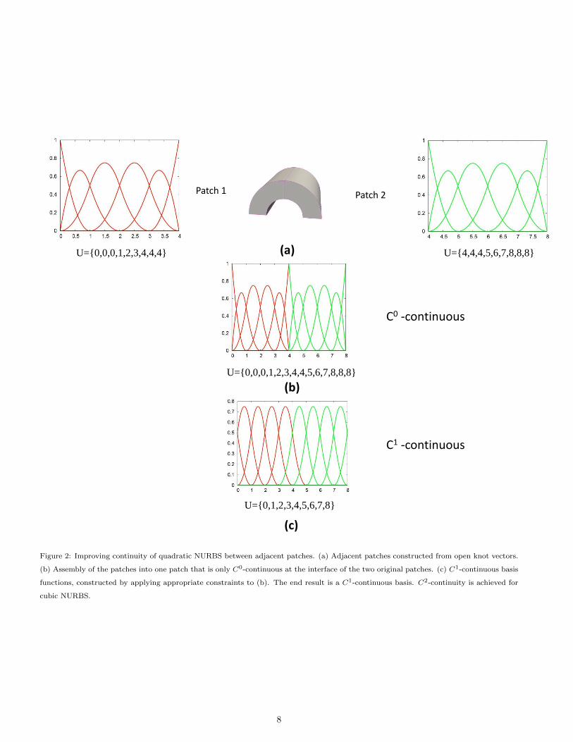
The basis functions used to represent flow variables (i.e., velocity and pressure) in the analyses are not the same as used

to construct the geometry. The objective is to form smooth periodic bases in the axial and cylindrical directions. This can

also be accomplished in several ways. The procedure we used is to start with smooth basis functions within each patch that

are only C0-continuous across patch interfaces and then apply constraint conditions that render them equally smooth across

interfaces. The idea is schematically illustrated in Figure 2 for quadratic NURBS. A globally C1-continuous basis is attained

thereby. Proceeding analogously, a C2-continuous basis may be constructed for cubic NURBS.

In one case, the laminar flow calculation of the next section, we also consider a standard trilinear hexahedral finite element

mesh for both the geometry and flow variables. In this case the geometry is only approximate in that the cylindrical surfaces

are approximated by flat rectangular facets.

7

Patch 1 Patch 2

C0 -continuous

C1 -continuous

(a)

(b)

(c)

U=0,0,0,1,2,3,4,4,5,6,7,8,8,8

U=0,1,2,3,4,5,6,7,8

U=4,4,4,5,6,7,8,8,8 U=0,0,0,1,2,3,4,4,4

Figure 2: Improving continuity of quadratic NURBS between adjacent patches. (a) Adjacent patches constructed from open knot vectors.

(b) Assembly of the patches into one patch that is only C0-continuous at the interface of the two original patches. (c) C1-continuous basis

functions, constructed by applying appropriate constraints to (b). The end result is a C1-continuous basis. C2-continuity is achieved for

cubic NURBS.

8

4. Laminar flow

This section describes a laminar verification of the numerical formulation. The flow is chosen as a test case because the exact

solution is available to compare with the numerical results. Mesh refinement studies are performed for each order of solution

approximation utilized, namely linear, quadratic, and cubic basis functions.

Flow direction

Figure 3: Laminar flow, snapshot of velocity contours for Re = 0.004, based on bulk-flow Reynolds number.

4.1. Problem setup

The flow domain is illustrated in Figure 3. A no slip Dirichlet boundary condition is set at the walls. The flow is driven by

a constant pressure gradient, fx , acting in the stream-wise direction. The values of the kinematic viscosity ν and the forcing fx

are set to 103 and 3.0, respectively.

4.2. Numerical results

The computations were performed on 163, 323 and 643 elements. We employ C0-continuous linear finite elements, and

C1-continuous quadratic and C2-continuous cubic NURBS. For all orders, the number of basis functions is equal to the number

of elements in the stream-wise and circumferential directions. In the wall-normal direction, due to the open knot vector

construction, the number of basis functions is n + p, where n is the number of elements in the wall-normal direction and p is

the polynomial order. Our numerical results are compared with the analytical solution, which is given in [51], namely,

u =1

4ν

(− dp

dx

)(Ro

2 −R2 +Ro

2 −Ri2

ln(Ri/Ro)lnRoR

)(32)

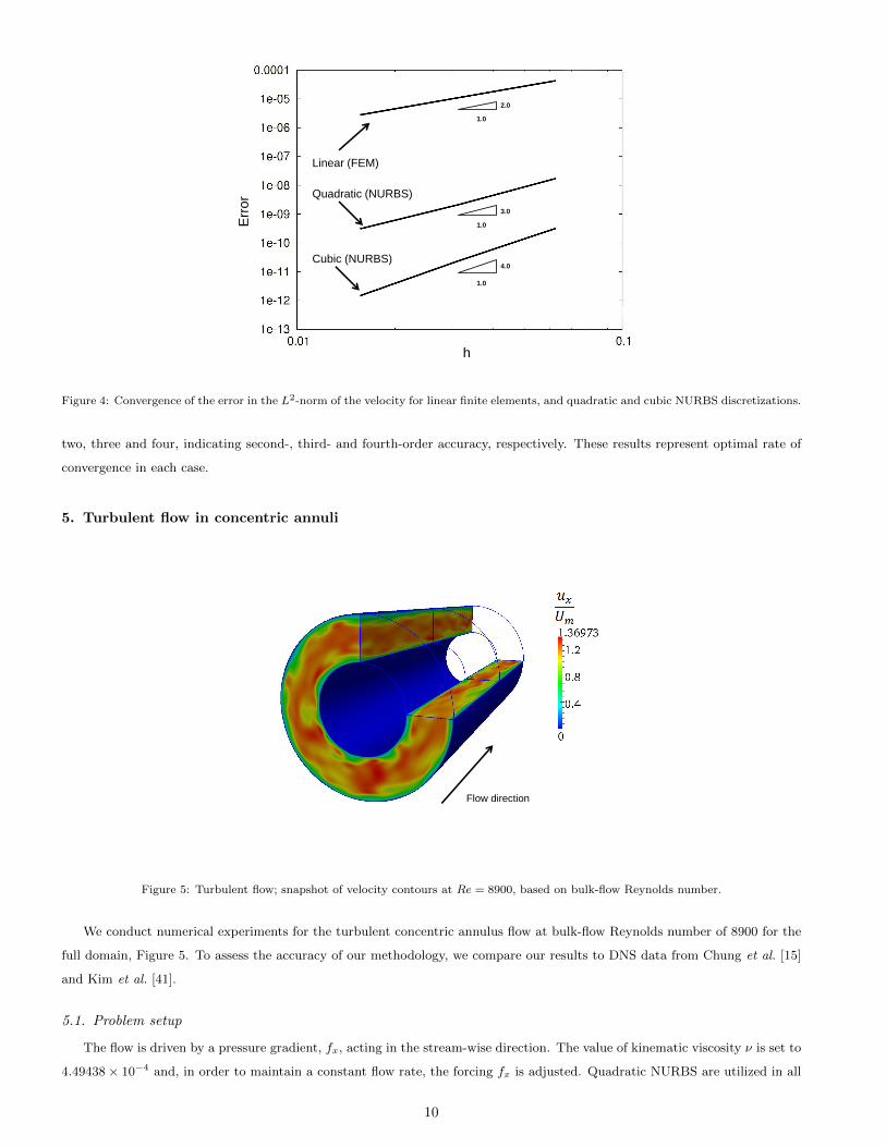
The rates of convergence of the error measured in the L2-norm of velocity versus mesh parameter, are presented in Figure

4. As may be seen in Figure 4, the slopes of the lines related to linear, quadratic and cubic approximations are approximately

9

h

Err

or

1.0

1.0

1.0

2.0

3.0

4.0

Quadratic (NURBS)

Cubic (NURBS)

Linear (FEM)

Figure 4: Convergence of the error in the L2-norm of the velocity for linear finite elements, and quadratic and cubic NURBS discretizations.

two, three and four, indicating second-, third- and fourth-order accuracy, respectively. These results represent optimal rate of

convergence in each case.

5. Turbulent flow in concentric annuli

Flow direction

Figure 5: Turbulent flow; snapshot of velocity contours at Re = 8900, based on bulk-flow Reynolds number.

We conduct numerical experiments for the turbulent concentric annulus flow at bulk-flow Reynolds number of 8900 for the

full domain, Figure 5. To assess the accuracy of our methodology, we compare our results to DNS data from Chung et al. [15]

and Kim et al. [41].

5.1. Problem setup

The flow is driven by a pressure gradient, fx, acting in the stream-wise direction. The value of kinematic viscosity ν is set to

4.49438× 10−4 and, in order to maintain a constant flow rate, the forcing fx is adjusted. Quadratic NURBS are utilized in all

10

the computations [30]. We perform our simulations using a sequence of h-refined meshes to assess the convergence properties of

the numerical methodology. The continuity of the basis functions is kept at C1, which is the maximal continuity achievable for

a quadratic NURBS discretization. We note that at each level of refinement, quadratic NURBS capture the problem geometry

exactly. The coarsest mesh computations were performed on a mesh of 64× 16× 16 elements in the circumferential, radial and

axial directions, respectively. With each h-refinement step we double the number of elements in each parametric direction to

achieve our finest discretization of 256× 64× 64 elements. A uniform mesh is used in the circumferential and axial directions.

In the radial direction, the meshes are obtained by distributing the knots according to a hyperbolic tangent function to better

capture the boundary layer turbulence.

Inner wall Outer wall

Chung et al. [15]

Figure 6: Mean axial velocity distribution normalized by the bulk velocity, Um, at Re = 8900.

11

Inner wall

Kim et al. [41]

Outer wall

Kim et al. [42]

Figure 7: Inner and outer wall mean velocity distributions at Re = 8900 computed using quadratic NURBS: h-refinement interpretation

of results. Here U+x = Ux

uτand y+ = yuτ

ν.

12

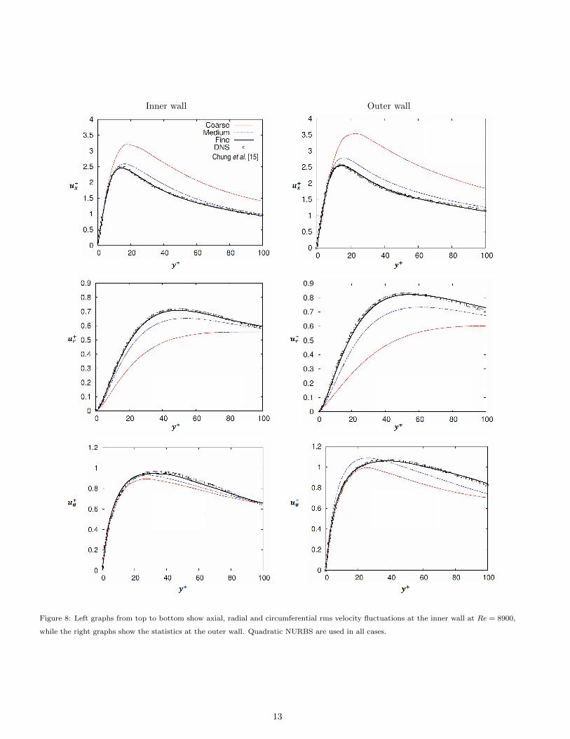
Inner wall Outer wall

Chung et al. [15] Chung et al. [15]

Chung et al. [15] Chung et al. [15]

Figure 8: Left graphs from top to bottom show axial, radial and circumferential rms velocity fluctuations at the inner wall at Re = 8900,

while the right graphs show the statistics at the outer wall. Quadratic NURBS are used in all cases.

13

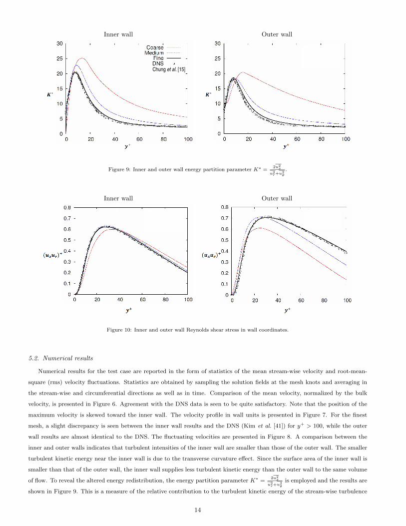
Inner wall Outer wall

Chung et al. [15]

Figure 9: Inner and outer wall energy partition parameter K∗ =2u2x

u2r+u2

θ

.

Inner wall Outer wall

Figure 10: Inner and outer wall Reynolds shear stress in wall coordinates.

5.2. Numerical results

Numerical results for the test case are reported in the form of statistics of the mean stream-wise velocity and root-mean-

square (rms) velocity fluctuations. Statistics are obtained by sampling the solution fields at the mesh knots and averaging in

the stream-wise and circumferential directions as well as in time. Comparison of the mean velocity, normalized by the bulk

velocity, is presented in Figure 6. Agreement with the DNS data is seen to be quite satisfactory. Note that the position of the

maximum velocity is skewed toward the inner wall. The velocity profile in wall units is presented in Figure 7. For the finest

mesh, a slight discrepancy is seen between the inner wall results and the DNS (Kim et al. [41]) for y+ > 100, while the outer

wall results are almost identical to the DNS. The fluctuating velocities are presented in Figure 8. A comparison between the

inner and outer walls indicates that turbulent intensities of the inner wall are smaller than those of the outer wall. The smaller

turbulent kinetic energy near the inner wall is due to the transverse curvature effect. Since the surface area of the inner wall is

smaller than that of the outer wall, the inner wall supplies less turbulent kinetic energy than the outer wall to the same volume

of flow. To reveal the altered energy redistribution, the energy partition parameter K∗ =2u2x

u2r+u2

θ

is employed and the results are

shown in Figure 9. This is a measure of the relative contribution to the turbulent kinetic energy of the stream-wise turbulence

14

Exactly the same procedures and code were used in all calculations, supporting the hypothesis that the variational multiscale

method is a general and accurate approach for solving the Navier-Stokes equations in all flow regimes. In the turbulent regime,

VMS exhibits features similar to an LES turbulence model, but achieves rapid convergence to a DNS. In the laminar regime, VMS

behaves like a higher-order accurate, residual-driven stabilized method. We believe these are distinguishing and advantageous

features of VMS when compared with classical LES turbulence modeling methods.

Acknowledgments

This research was supported by WCU (World Class University) program through the National Research Foundation of

Korea funded by the Ministry of Education, Science and Technology(#R33-10150), and also Basic Science Research Program

through the National Research Foundation of Korea funded by the Ministry of Education, Science and Technology(#2009-

0065381,#2010-0004606). The authors would like to acknowledge the support from KISTI supercomputing center through the

strategic support program for the supercomputing application research(#KSC-2010-C2-0013).

Appendix A. Geometry construction.

The cylinder shown in Figure 1 has an inner radius of Ri = 2, and an outer radius of Ro = 4. The length of the cylinder

is L = 18. Quadratic NURBS are used in all direction. The u3 coordinate traverses the circumferential direction; the u2

coordinate traverses the thickness, and the u1 coordinate traverses the length. Table A.1 represents the knot vectors for the 8

patches.

Table A.1: Knot vectors for cylindrical solid

Patch no. U1 U2 U3

1 0,0,0,1,1,1 0,0,0,1,1,1 0,0,0,1,1,1

2 1,1,1,2,2,2 0,0,0,1,1,1 0,0,0,1,1,1

3 0,0,0,1,1,1 0,0,0,1,1,1 1,1,1,2,2,2

4 1,1,1,2,2,2 0,0,0,1,1,1 1,1,1,2,2,2

5 0,0,0,1,1,1 0,0,0,1,1,1 2,2,2,3,3,3

6 1,1,1,2,2,2 0,0,0,1,1,1 2,2,2,3,3,3

7 0,0,0,1,1,1 0,0,0,1,1,1 3,3,3,4,4,4

8 1,1,1,2,2,2 0,0,0,1,1,1 3,3,3,4,4,4

The control net and weights are given in Tables A.2 - A.9 . Rational solid basis functions are defined by combining the

weights and one-dimensional basis functions using (A.1),

Rp,q,ri,j,k (u1, u2, u3) =Ni,p(u1)Mj,q(u2)Lk,r(u3)wi,j,k

n∑i=0

m∑j=0

l∑k=0

Ni,p(u1)Mj,q(u2)Lk,r(u3)wijk

(A.1)

The number of control points are n, m, and l in the axial, radial and circumferential directions, repectively. The N ,M ,L, w

represent the basis functions in each direction and the weight, and p, q, r are the polynomial orders in each direction.

16

Table A.2: Control points and weights for cylindrical solid, patch no.1

j k B0,j,k B1,j,k B2,j,k w0,j,k w1,j,k w2,j,k

0 0 (0,0,2) (9/2,0,2) (9,0,2) 1 1 1

1 0 (0,0,3) (9/2,0,3) (9,0,3) 1 1 1

2 0 (0,0,4) (9/2,0,4) (9,0,4) 1 1 1

0 1 (0,2,2) (9/2,2,2) (9,2,2) 1/√

2 1/√

2 1/√

2

1 1 (0,3,3) (9/2,3,3) (9,3,3) 1/√

2 1/√

2 1/√

2

2 1 (0,4,4) (9/2,4,4) (9,4,4) 1/√

2 1/√

2 1/√

2

0 2 (0,2,0) (9/2,2,0) (9,2,0) 1 1 1

1 2 (0,3,0) (9/2,3,0) (9,3,0) 1 1 1

2 2 (0,4,0) (9/2,4,0) (9,4,0) 1 1 1

Table A.3: Control points and weights for cylindrical solid, patch no.2

j k B0,j,k B1,j,k B2,j,k w0,j,k w1,j,k w2,j,k

0 0 (9,0,2) (27/2,0,2) (18,0,2) 1 1 1

1 0 (9,0,3) (27/2,0,3) (18,0,3) 1 1 1

2 0 (9,0,4) (27/2,0,4) (18,0,4) 1 1 1

0 1 (9,2,2) (27/2,2,2) (18,2,2) 1/√

2 1/√

2 1/√

2

1 1 (9,3,3) (27/2,3,3) (18,3,3) 1/√

2 1/√

2 1/√

2

2 1 (9,4,4) (27/2,4,4) (18,4,4) 1/√

2 1/√

2 1/√

2

0 2 (9,2,0) (27/2,2,0) (18,2,0) 1 1 1

1 2 (9,3,0) (27/2,3,0) (18,3,0) 1 1 1

2 2 (9,4,0) (27/2,4,0) (18,4,0) 1 1 1

Table A.4: Control points and weights for cylindrical solid, patch no.3

j k B0,j,k B1,j,k B2,j,k w0,j,k w1,j,k w2,j,k

0 0 (0,2,0) (9/2,2,0) (9,2,0) 1 1 1

1 0 (0,3,0) (9/2,3,0) (9,3,0) 1 1 1

2 0 (0,4,0) (9/2,4,0) (9,4,0) 1 1 1

0 1 (0,2,-2) (9/2,2,-2) (9,2,-2) 1/√

2 1/√

2 1/√

2

1 1 (0,3,-3) (9/2,3,-3) (9,3,-3) 1/√

2 1/√

2 1/√

2

2 1 (0,4,-4) (9/2,4,-4) (9,4,-4) 1/√

2 1/√

2 1/√

2

0 2 (0,0,-2) (9/2,0,-2) (9,0,-2) 1 1 1

1 2 (0,0,-3) (9/2,0,-3) (9,0,-3) 1 1 1

2 2 (0,0,-4) (9/2,0,-4) (9,0,-4) 1 1 1

17

Table A.5: Control points and weights for cylindrical solid, patch no.4

j k B0,j,k B1,j,k B2,j,k w0,j,k w1,j,k w2,j,k

0 0 (9,2,0) (27/2,2,0) (18,2,0) 1 1 1

1 0 (9,3,0) (27/2,3,0) (18,3,0) 1 1 1

2 0 (9,4,0) (27/2,4,0) (18,4,0) 1 1 1

0 1 (9,2,-2) (27/2,2,-2) (18,2,-2) 1/√

2 1/√

2 1/√

2

1 1 (9,3,-3) (27/2,3,-3) (18,3,-3) 1/√

2 1/√

2 1/√

2

2 1 (9,4,-4) (27/2,4,-4) (18,4,-4) 1/√

2 1/√

2 1/√

2

0 2 (9,0,-2) (27/2,0,-2) (18,0,-2) 1 1 1

1 2 (9,0,-3) (27/2,0,-3) (18,0,-3) 1 1 1

2 2 (9,0,-4) (27/2,0,-4) (18,0,-4) 1 1 1

Table A.6: Control points and weights for cylindrical solid, patch no.5

j k B0,j,k B1,j,k B2,j,k w0,j,k w1,j,k w2,j,k

0 0 (0,0,-2) (9/2,0,-2) (9,0,-2) 1 1 1

1 0 (0,0,-3) (9/2,0,-3) (9,0,-3) 1 1 1

2 0 (0,0,-4) (9/2,0,-4) (9,0,-4) 1 1 1

0 1 (0,-2,-2) (9/2,-2,-2) (9,-2,-2) 1/√

2 1/√

2 1/√

2

1 1 (0,-3,-3) (9/2,-3,-3) (9,-3,-3) 1/√

2 1/√

2 1/√

2

2 1 (0,-4,-4) (9/2,-4,-4) (9,-4,-4) 1/√

2 1/√

2 1/√

2

0 2 (0,-2,0) (9/2,-2,0) (9,-2,0) 1 1 1

1 2 (0,-3,0) (9/2,-3,0) (9,-3,0) 1 1 1

2 2 (0,-4,0) (9/2,-4,0) (9,-4,0) 1 1 1

Table A.7: Control points and weights for cylindrical solid, patch no.6

j k B0,j,k B1,j,k B2,j,k w0,j,k w1,j,k w2,j,k

0 0 (9,0,-2) (27/2,0,-2) (18,0,-2) 1 1 1

1 0 (9,0,-3) (27/2,0,-3) (18,0,-3) 1 1 1

2 0 (9,0,-4) (27/2,0,-4) (18,0,-4) 1 1 1

0 1 (9,-2,-2) (27/2,-2,-2) (18,-2,-2) 1/√

2 1/√

2 1/√

2

1 1 (9,-3,-3) (27/2,-3,-3) (18,-3,-3) 1/√

2 1/√

2 1/√

2

2 1 (9,-4,-4) (27/2,-4,-4) (18,-4,-4) 1/√

2 1/√

2 1/√

2

0 2 (9,-2,0) (27/2,-2,0) (18,-2,0) 1 1 1

1 2 (9,-3,0) (27/2,-3,0) (18,-3,0) 1 1 1

2 2 (9,-4,0) (27/2,-4,0) (18,-4,0) 1 1 1

18

Table A.8: Control points and weights for cylindrical solid, patch no.7

j k B0,j,k B1,j,k B2,j,k w0,j,k w1,j,k w2,j,k

0 0 (0,-2,0) (9/2,-2,0) (9,-2,0) 1 1 1

1 0 (0,-3,0) (9/2,-3,0) (9,-3,0) 1 1 1

2 0 (0,-4,0) (9/2,-4,0) (9,-4,0) 1 1 1

0 1 (0,-2,2) (9/2,-2,2) (9,-2,2) 1/√

2 1/√

2 1/√

2

1 1 (0,-3,3) (9/2,-3,3) (9,-3,3) 1/√

2 1/√

2 1/√

2

2 1 (0,-4,4) (9/2,-4,4) (9,-4,4) 1/√

2 1/√

2 1/√

2

0 2 (0,0,2) (9/2,0,2) (9,0,2) 1 1 1

1 2 (0,0,3) (9/2,0,3) (9,0,3) 1 1 1

2 2 (0,0,4) (9/2,0,4) (9,0,4) 1 1 1

Table A.9: Control points and weights for cylindrical solid, patch no.8

j k B0,j,k B1,j,k B2,j,k w0,j,k w1,j,k w2,j,k

0 0 (9,-2,0) (27/2,-2,0) (18,-2,0) 1 1 1

1 0 (9,-3,0) (27/2,-3,0) (18,-3,0) 1 1 1

2 0 (9,-4,0) (27/2,-4,0) (18,-4,0) 1 1 1

0 1 (9,-2,2) (27/2,-2,2) (18,-2,2) 1/√

2 1/√

2 1/√

2

1 1 (9,-3,3) (27/2,-3,3) (18,-3,3) 1/√

2 1/√

2 1/√

2

2 1 (9,-4,4) (27/2,-4,4) (18,-4,4) 1/√

2 1/√

2 1/√

2

0 2 (9,0,2) (27/2,0,2) (18,0,2) 1 1 1

1 2 (9,0,3) (27/2,0,3) (18,0,3) 1 1 1

2 2 (9,0,4) (27/2,0,4) (18,0,4) 1 1 1

References

[1] Akkerman I, Bazilevs Y, Calo VM , Hughes TJR, Hulshof S. The role of continuity in residual-based variational multiscale

modeling of turbulence. Computational Mechanics 2008;41:371-78.

[2] Auricchio F, Beirao de Veiga L, Buffa A, Lovadina C, Reali A, Sangalli G. A fully ”locking-free” isogeometric approach for

plane linear elasticity problems: A stream function formulation. Comput Methods Appl Mech Eng 2007;197:160-72.

[3] Auricchio F, Beirao de Veiga L, Lovadina C, Reali A. The importance of the exact satisfaction of the incompressibility

constraint in nonlinear elasticity: mixed FEMs versus NURBS-based approximations. Comput Methods Appl Mech Eng

2010;199:314-23.

[4] Azouz I, Shirazi SA. Evaluation of several turbulence models for turbulent flow in concentric and eccentric annuli, ASME

J Energy Resources Tech 1998;120:268-75.

[5] Bazilevs Y, Beirao de Veiga L, Cottrell JA, Hughes TJR, Sangalli G. Isogeometric analysis: approximation, stability and

error estimates for h-refine meshes. Mathematical Models and Methods in Applied Science 2006;16:1-60.

19

[6] Bazilevs Y, Calo VM, Cottrell JA, Hughes TJR, Reali A, Scovazzi G. Variational multiscale residual-based turbulence

modeling for large eddy simulation of incompressible flows. Comput Methods Appl Mech Eng 2007;197:173-201.

[7] Bazilevs Y, Calo VM, Zhang JY, Hughes TJR. Isogeometric Fluid-Structure Interaction Analysis with Applications to

Arterial Blood Flow. Computational Mechanics 2006;38:310-22.

[8] Bazilevs Y, Michler C, Calo VM, Hughes TJR. Weak Dirichlet boundary conditions for wall-bounded turbulent flows.

Comput Methods Appl Mech Eng 2007;196:4853-62.

[9] Bazilevs Y, Michler C, Calo VM, Hughes TJR. Isogeometric variational multiscale modeling of wall-bounded turbulent

flows with weakly-enforced boundary conditions on unstretched meshes. Comput Methods Appl Mech Eng 2010;199:780-90.

[10] Brooks AN, Hughes TJR. Streamline upwind/Petrov-Galerkin formulations for convection dominated flows with particular

emphasis on the incompressible Navier-Stokes equations. Comput Methods Appl Mech Eng 1982;32:199-259.

[11] Calo VM. Residual-based Multiscale Turbulence Modeling: Finite Volume Simulation of Bypass Transition. PhD thesis,

Department of Civil and Environmental Engineering, Standford University, 2004.

[12] Calo VM, Brasher N, Bazilevs Y, Hughes TJR. Multiphysics Model for Blood Flow and Drug Transport with Application

to Patient-Specific Coronary Artery Flow. Computational Mechanics 2008;43:161-177.

[13] Chang K, Hughes TJR, Calo VM. Isogeometric Variational Multiscale Large-Eddy Simulation of Fully-developed Turbulent

Flow over a Wavy Wall. Computers and Fluids 2011; submitted.

[14] Chung J, Hulbert GM. A time integration algorithm for structural dynamics with improved numerical dissipation: the

generalized alpha-method. J Appl Mech 1993;60:371-75.

[15] Chung SY, Rhee GH, Sung HJ. Direct numerical simulation of turbulent concentric annular pipe flow Part 1: Flow field,

Int J Heat and Fluid Flow 2002;23:426-40.

[16] Codina R, Principe J, Guasch O, Badia S. Time dependent subscales in the stabilized finite element approximation of

incompressible flow problems. Comput Methods Appl Mech Eng 2007;196:2413-30.

[17] Collier NO, Pardo D, Paszynski M, Dalcın L, Calo VM. The cost of continuity: a study of the performance of isogeometric

finite elements using direct solvers. Comput Methods Appl Mech Eng 2012; accepted for publication.

[18] Cottrell JA, Hughes TJR, Bazilevs Y. Isogeometric Analysis, Towards integration of CAD and FEA. Wiley, 2009.

[19] Cottrell JA, Hughes TJR, Reali A. Studies of Refinement and Continuity in Isogeometric Structural Analysis. Comput

Methods Appl Mech Eng 2007;196:4160-83.

[20] Dede L, Borden MJ, Hughes TJR. Isogeometric Analysis for topology optimization with a phase field model, ICES Report

11-29, The Institute for Computational Engineering and Sciences, The University of Texas at Austin 2011, Archives of

Computational Methods in Engineering, accepted for publication.

[21] Duddu R, Lavier L, Hughes TJR, Calo VM. A finite strain Eulerian formulation for compressible and nearly incompressible

hyper-elasticity using high-order NURBS elements. International Journal of Numerical Methods in Engineering 2012;

89:762-785.

[22] Escudier MP, Gouldson IW, Jones DM. Flow of shear-thinning fluids in a concentric annulus. Experiments in Fluids

1995;27:225-38.

20

[23] Gomez H, Calo VM, Bazilevs Y, Hughes TJR. Isogeometric analysis of the Cahn-Hilliard phase-field model. Comput

Methods Appl Mech Eng 2008;197:4333-4352.

[24] Gomez H, Hughes TJR, Nogueira X, Calo VM. Isogeometric analysis of the isothermal Navier-Stokes-Korteweg equations.

Comput Methods Appl Mech Eng 2010;199:1828.

[25] Holmen J, Hughes TJR, Oberai AA, Wells GN. Sensitivity of the scale partition for variational multiscale LES of channel

flow. Phys Fluids 2004;16:824-27.

[26] Hossain S, Hossainy SFA, Bazilevs Y, Calo VM, Hughes TJR. Mathematical Modeling of Coupled Drug and Drug-

Encapsulated Nanoparticle Transport in Patient-Specific Coronary Artery Walls. Computational Mechanics 2011; doi:

10.1007/s00466-011-0633-2.

[27] Hsu MC, Akkerman I, Bazilevs Y. High-performance computing of wind turbine aerodynamics using isogeometric analysis.

Computers and Fluids 2011;49:93-100.

[28] Hughes TJR. Multiscale phenomena: Green functions, the Dirichlet-to-Neumann formulation, subgrid scale models, bubbles

and the origins of stabilized methods. Comput Methods Appl Mech Eng 1995;127:387-401.

[29] Hughes TJR, Calo VM, Scovazzi G. Variational and multiscale methods in turbulence, in: W.Gutkowski,T.A. Kowalewski

(Eds.), Proceedings of the XXI International Congress of Theoretical and Applied Mechanics (IUTAM), Kluwer, 2004.

[30] Hughes TJR, Cottrell JA, Bazilevs Y. Isogeometric analysis: CAD, finite elements, NURBS, exact geometry, and mesh

refinement. Comput Methods Appl Mech Eng 2005;194:4135-95.

[31] Hughes TJR, Franca LP, Hulbert G. A new finite element formulation for computational fluid dynamics: VIII. The Galerkin

least squares method for advective-diffusive equations. Comput Methods Appl Mech Eng 1989;73:173-89.

[32] Hughes TJR, Mallet M. A few finite element formulation for fluid dynamics: III. The generalized streamline operator for

multidimensional advective-diffusive systems. Comput Methods Appl Mech Eng 1986;58:305-28.

[33] Hughes TJR, Mazzei L, Jansen KE. Large-eddy simulation and the variational multiscale method. Comp Vis Sci 2000;3:47-

59.

[34] Hughes TJR, Mazzei L, Oberai AA, Wray AA. The multiscale formulation of large eddy simulation: decay of homogenous

isotropic turbulence. Phys Fluids 2001;13:505-12.

[35] Hughes TJR, Oberai AA, Mazzei L. Large eddy simulation of turbulent channel flows by the variational multiscale method.

Phys Fluids 2001;13:1784-99.

[36] Hughes TJR, Reali A, Sangalli G. Duality and Unified Analysis of Discrete Approximations in Structural Dynamics and

Wave Propagation: Comparison of p-method Finite Elements with k-method NURBS. Comput Methods Appl Mech Eng

2008;197:4104-24.

[37] Hughes TJR, Sangalli G. Variational multiscale analysis: The fine-scale Green’s function, projection, optimization, local-

ization, and stabilized methods. SIAM Journal on Numerical Analysis 2007;45:539-57.

[38] Hughes TJR, Scovazzi G, Franca LP. Multiscale and stabilized methods, in: E. Stein, R. de Borst, T.J.R. Hughes (Eds.),

Encyclopedia of Computational Mechanics, Computational Fluid Dynamics,Vol. 3, Wiley, 2004.

21

[39] Hughes TJR , Wells GN, Oberai AA, Wray AA. Energy transfers and spectral eddy viscosity of homogeneous isotropic turbu-

lence: comparison of dynamic Smagorinsky and multiscale models over a range of discretizations. Phys Fluids 2004;16:4044-

52.

[40] Jansen KE, Whiting CH, Hulbert GM. A generalized alpha-method for integrating the filtered Navier–Stokes equations

with a stabilized finite element method. Comput Methods Appl Mech Eng 1999;190:305-19.

[41] Kim J, Moin P, Moser R. Turbulent statistics in fully developed channel at low Reynolds number, J Fluid Mech

1987;177:617-41.

[42] Koobus B, Farhat C. A variational multiscale method for the large eddy simulation of compressible turbulent flow on

unstructed meshes – applications to vortex shedding. Comput Methods Appl Mech Eng 2004;193:1367-83.

[43] Lawn CJ, Elliott CJ. Fully Developed Turbulent Flow through Concentric Annuli, Central Electricity Generating Board

Report RD/B/N/1878, United Kingdom, 1971.

[44] Liu NS, Lu XY. Large eddy simulation of turbulent concentric annular channel flows. Int J Num Meth Fluids 2004;45:1317-

38.

[45] Nouri JM, Umur H, Whitelaw JH. Flow of Newtonian and non-Newtonian fluids in concentric and eccentric annuli. J Fluid

Mech 1993;253:617-41.

[46] Piegl L, Tiller W. The NURBS book, Monographs in visual communication, second ed., Springer-Verlag, New York, 1997.

[47] Ramakrishnan S, Collis SS. Turbulent control simulation using the variational multiscale method. AIAA journal

2004;42:745-53;

[48] Reali A. An isogeometric analysis approach for the study structural vibrations. Journal of Earthquake Engineering

2006;10:1-30.

[49] Rehme K. Turbulence measurements in smooth concentric annuli with small radius ratios. J Fluid Mech 1975;72:189-206.

[50] Verhoosel CV, Scott MA, Hughes TJR, de Borst R. An isogeometric analysis approach to gradient damage models. Inter-

national Journal for Numerical Methods in Engineering 2011;86:115134.

[51] White FM. Fluid Mechanics, third ed., Mc Graw–Hill, New York, 1994.

[52] Zhang Y, Bazilevs Y, Goswami S, Bajaj CL, Hughes TJR. Patient-specific vascular NURBS modeling for isogeometric

analysis of blood flow. Comput Methods Appl Mech Eng 2007;196:2943-59.

22