Identifying Deviating Systems with Unsupervised …238364/FULLTEXT01.pdfIdentifying Deviating...

Technical Report, IDE0801, January 2008

Identifying Deviating Systems withUnsupervised Learning

Master Thesis in

Computer Systems Engineering

Georg Panholzer

School of Information Science, Computer and Electrical EngineeringHalmstad University

Identifying Deviating Systems withUnsupervised Learning

School of Information Science, Computer and Electrical EngineeringHalmstad University

Box 823, S-301 18 Halmstad, Sweden

January 2008

Acknowledgement

Everything makes sense a bit at a time. But when you tryto think of it all at once, it comes out wrong.

Terence David John Pratchett

First of all I want to thank my supervisor Prof. Thorsteinn Rognvaldsson, whose advicesand suggestions helped me during the whole time of preparing and writing this thesis.

I also want to thank my parents for providing me the possibility to study abroad.

Special thanks goes to Stephanie for all her love, patience and encouragement.

The cover illustration is generously provided by Sharon Rosa.

The motion capturing data set “CMU Database” was obtained from http://mocap.cs.

cmu.edu. The database was created with funding from NSF EIA-0196217.

The motion capturing data set “MIT Data set” was obtained from http://people.

csail.mit.edu/ehsu/work/sig05stf.

iii

http://mocap.cs.cmu.edu

http://mocap.cs.cmu.edu

http://people.csail.mit.edu/ehsu/work/sig05stf

http://people.csail.mit.edu/ehsu/work/sig05stf

Details

First Name, Surname: Georg PanholzerUniversity: Halmstad University, SwedenDegree Program: Computer Systems EngineeringTitle of Thesis: Identifying Deviating Systems with Unsupervised LearningAcademic Supervisor: Prof. Thorsteinn Rognvaldsson

Abstract

We present a technique to identify deviating systems among a group of systems in aself-organized way. A compressed representation of each system is used to computesimilarity measures, which are combined in an affinity matrix of all systems. Deviationdetection and clustering is then used to identify deviating systems based on this affinitymatrix.

The compressed representation is computed with Principal Component Analysis andKernel Principal Component Analysis. The similarity measure between two compressedrepresentations is based on the angle between the spaces spanned by the principalcomponents, but other methods of calculating a similarity measure are suggested aswell. The subsequent deviation detection is carried out by computing the probability ofeach system to be observed given all the other systems. Clustering of the systems isdone with hierarchical clustering and spectral clustering.

The whole technique is demonstrated on four data sets of mechanical systems, two of asimulated cooling system and two of human gait. The results show its applicability onthese mechanical systems.

Keywords

Deviation Detection, Clustering, Eigen-Subspace, Machine Learning

v

Contents

Acknowledgement iii

Details v

Abstract v

Keywords v

Contents vii

List of Figures xi

List of Tables xiii

1 Introduction 1

1.1 Problem formulation . . . . . . . . . . . . . . . . . . . . . . . . . . . . 3

2 Background 5

3 Methods 9

3.1 System representation . . . . . . . . . . . . . . . . . . . . . . . . . . . 9

3.1.1 Feature Extraction . . . . . . . . . . . . . . . . . . . . . . . . . 10

3.1.2 Principal Components Analysis . . . . . . . . . . . . . . . . . . 10

3.1.2.1 Calculation of the Principal Components . . . . . . . . 11

3.1.3 Kernel Principal Components Analysis . . . . . . . . . . . . . . 12

3.1.3.1 The Kernel Trick . . . . . . . . . . . . . . . . . . . . . 12

3.1.3.2 Calculation of the Kernel Principal Components . . . . 14

3.1.4 Other nonlinear PCA methods . . . . . . . . . . . . . . . . . . . 15

3.2 System comparison . . . . . . . . . . . . . . . . . . . . . . . . . . . . . 15

vii

3.2.1 Calculation of the Angle between two Subspaces . . . . . . . . . 17

3.2.2 The Affinity Matrix . . . . . . . . . . . . . . . . . . . . . . . . . 18

3.3 Deviation detection . . . . . . . . . . . . . . . . . . . . . . . . . . . . . 18

3.3.1 Bootstrapping . . . . . . . . . . . . . . . . . . . . . . . . . . . . 20

3.4 Clustering . . . . . . . . . . . . . . . . . . . . . . . . . . . . . . . . . . 20

3.4.1 Spectral Clustering . . . . . . . . . . . . . . . . . . . . . . . . . 21

3.4.2 Hierarchical Clustering . . . . . . . . . . . . . . . . . . . . . . . 22

4 Data sets 25

4.1 Vehicle Cooling System . . . . . . . . . . . . . . . . . . . . . . . . . . . 25

4.1.1 Healthy Systems . . . . . . . . . . . . . . . . . . . . . . . . . . 26

4.1.2 Systems with a Leakage . . . . . . . . . . . . . . . . . . . . . . 26

4.1.3 Soiled Systems . . . . . . . . . . . . . . . . . . . . . . . . . . . 26

4.2 Human Gait Data . . . . . . . . . . . . . . . . . . . . . . . . . . . . . . 26

4.2.1 CMU Data Set . . . . . . . . . . . . . . . . . . . . . . . . . . . 27

4.2.2 MIT Data Set . . . . . . . . . . . . . . . . . . . . . . . . . . . . 28

5 Results and Discussions 31

5.1 Deviation detection . . . . . . . . . . . . . . . . . . . . . . . . . . . . . 31

5.1.1 Cooling System with a Leakage . . . . . . . . . . . . . . . . . . 31

5.1.1.1 Deviation Detection based on PCA . . . . . . . . . . . 31

5.1.1.2 Detection Performance with Erroneous Normals . . . . 33

5.1.1.3 Deviation Detection based on Kernel PCA . . . . . . . 35

5.1.2 Soiled Cooling System . . . . . . . . . . . . . . . . . . . . . . . 35

5.1.3 Human Gait Data - CMU Data Set . . . . . . . . . . . . . . . . 36

5.1.4 Human Gait Data - MIT Data Set . . . . . . . . . . . . . . . . 37

5.2 Clustering . . . . . . . . . . . . . . . . . . . . . . . . . . . . . . . . . . 40

5.2.1 Cooling System with a Leakage . . . . . . . . . . . . . . . . . . 40

5.2.1.1 Spectral Clustering on PCA . . . . . . . . . . . . . . . 40

5.2.1.2 Hierarchical Clustering on PCA . . . . . . . . . . . . . 43

5.2.1.3 Clustering on KPCA . . . . . . . . . . . . . . . . . . . 44

5.2.2 Soiled Cooling System . . . . . . . . . . . . . . . . . . . . . . . 46

5.2.2.1 Clustering on PCA . . . . . . . . . . . . . . . . . . . . 46

viii


5.2.3 Human Gait Data - CMU Data Set . . . . . . . . . . . . . . . . 49



5.2.4 Human Gait Data - MIT Data Set . . . . . . . . . . . . . . . . 50


6 Summary and Conclusion 51

Bibliography 53

Appendix 57

A.1 Cooling System with a Leakage: Spectral Clustering on PCA . . . . . . 57

ix

List of Figures

3.1 Example of PCA . . . . . . . . . . . . . . . . . . . . . . . . . . . . . . 11

3.2 Example of kernel PCA with a Gaussian kernel . . . . . . . . . . . . . 13

3.3 Calculation of P (x|S) . . . . . . . . . . . . . . . . . . . . . . . . . . . 19

3.4 Effect of Bootstrapping . . . . . . . . . . . . . . . . . . . . . . . . . . . 20

3.5 Example of Spectral Clustering . . . . . . . . . . . . . . . . . . . . . . 21

3.6 Hierarchical clustering with the Macnaughton-Smith approach . . . . . 23

4.1 Example skeleton of the CMU data set . . . . . . . . . . . . . . . . . . 27

4.2 Example skeleton of the MIT data set . . . . . . . . . . . . . . . . . . . 29

5.1 Reconstruction Error against Principal Components . . . . . . . . . . . 32

5.2 Results of bootstrapping on normal systems . . . . . . . . . . . . . . . 33

5.3 Detection rate with erroneous samples in the “normals” set . . . . . . . 34

5.4 Affinity matrices of the MIT data set . . . . . . . . . . . . . . . . . . . 39

5.5 Affinity matrix and groupings against the number of clusters, PCA . . 41

5.6 Results of spectral clustering for the leakage data set, PCA . . . . . . . 42

5.7 Hierarchical clustering into 3 groups . . . . . . . . . . . . . . . . . . . . 43

5.8 Affinity matrix and groupings against the number of clusters, KPCA . 45

5.9 Results of spectral clustering for the leakage data set, KPCA . . . . . . 45

5.10 Hierarchical Clustering of the Soiled Cooling System . . . . . . . . . . 48

5.11 Hierarchical clustering of the CMU data set . . . . . . . . . . . . . . . 49

5.12 Hierarchical clustering of the MIT data set . . . . . . . . . . . . . . . . 50

A.1 Grouping probabilities for 2 groups . . . . . . . . . . . . . . . . . . . . 57

A.2 Grouping probabilities for 3 groups . . . . . . . . . . . . . . . . . . . . 58

A.3 Grouping probabilities for 4 groups: Group 1 . . . . . . . . . . . . . . . 59




xi

List of Tables

4.1 CMU Data Set subjects and trials . . . . . . . . . . . . . . . . . . . . 27

4.2 MIT Data set subjects and trials . . . . . . . . . . . . . . . . . . . . . 28

5.1 Results of bootstrapping on normal systems . . . . . . . . . . . . . . . 32

5.2 Results of bootstrapping on “faulty” systems, Leakage data . . . . . . . 33

5.3 Detection performance with erroneous samples in the “normals” set,mean affinity . . . . . . . . . . . . . . . . . . . . . . . . . . . . . . . . 34

5.4 Detection performance with erroneous samples in the “normals” set,separate affinities . . . . . . . . . . . . . . . . . . . . . . . . . . . . . . 35

5.5 Results of bootstrapping on “faulty” systems, Soil data . . . . . . . . . 36

5.6 Results of bootstrapping on the CMU data set . . . . . . . . . . . . . . 37

5.7 Detection Performance on the CMU data set . . . . . . . . . . . . . . . 37

5.8 Results of bootstrapping on the 12 “normals” of the MIT data set . . . 38

5.9 Results of bootstrapping on the “faulty” system, MIT data set . . . . . 38

5.10 Results of bootstrapping, Normals + Jog vs. Rest . . . . . . . . . . . . 39

xiii

1

Introduction

Today’s mechatronical systems like vehicles, robots or planes include a vast amount of

embedded systems that are used to control and monitor their actions. About 100 micro

processors and more than 2000 sensors are built into modern luxury-class cars. While

some control safety-critical systems like breaks or airbags, others are essential to run

the car, e.g. the engine control unit (ECU) which is responsible for fuel injection, spark

time etc.

Each of these microprocessors logs its measurements and actions. This enables manu-

facturers and operators to collect exact data about the runtime behavior, which can

then be used to find patterns (e.g. abnormalities after a certain sequence of events)

that help to precisely identify faults and their sources. Precise findings facilitate to

choose suitable counteractions and adapt service intervals, predict lifecycles and increase

productivity.

On the other hand, a huge amount of data is produced. Generally this data is very

complex and so specialized personnel and a lot of time is required to to have the data

analyzed. Hence, automatic systems are needed to take over or ease this task.

Such systems have to follow certain constraints:

• A compressed representation of the raw data is essential to reduce the amount of

data. This reduces transmission time which allows to use transmission techniques

with low bandwidth (e.g. wireless transmission) and also results in a better

scalability to a big number of systems.

1

2 1. Introduction

• The system has to be able to detect deviations that have not occurred before,

as it is (almost) impossible to think of all possible states beforehand. Thus, the

system has to be self-organizing to adapt to the parameters of the monitored

system automatically.

A lot of different forms of deviation detection methods have been used with a very

wide variety of tasks either to clean data for further usage or detect faulty systems

and behavior patterns. Depending on the author and field of application they are,

for example, called deviation detection, outlier detection, novelty detection, anomaly

detection, noise detection or exception mining. We will use the term deviation detection,

as we feel that this most appropriately describes the process of finding systems that

behave differently from a group of systems.

When used to clean data for further usage it is most often referred to as outlier detection.

In machine learning and data analysis this is done to remove observations that are either

erroneous (due to e.g. a faulty sensor) or normal measurements of a rare condition that

is under-represented in the data set and difficult to derive an exact model for. Including

observations of both cases generally results in a worse model of the actual data. Outlier

detection and removal is often done by visual inspection of histograms, box plots or

scatter plots. More sophisticated techniques include supervised classification, where

data known to be normal or abnormal is pre-labeled. Classifiers are built upon these

data and then used to classify the rest of the data.

Another application of deviation detection is to detect faulty systems or deviating

behavior patterns. This is often a very important task as deviations could indicate

faulty conditions which can lead to severe damage or even result in danger for users.

Also it might point out fraudulent usage or decreased performance. Of course under any

of those conditions it is beneficial to have a system that automatically detects deviating

systems.

In either way most deviation detection systems are designed for a specific purpose.

1.1. Problem formulation 3

1.1 Problem formulation

The goal of this thesis is to show that it is possible to detect “abnormal” systems in

a group of systems without much prior knowledge about the systems. The proposed

approach works offline, i.e. the whole data set is available before processing, but can be

extended to an online version.

The approach is based on the assumption that “abnormal” systems deviate from

“normal” systems if an appropriate representation is used. Deviating systems are those

which do not behave like the bulk of systems. The challenges are to find such an

appropriate representation in a self-organized way, compare these representation and

then detect deviations.

The task is divided into three sub-tasks:

1. How to represent an individual system?

This step extracts features that are “important”, i.e. those components that

describe the systems behavior. The outcome of this step is a more efficient

representation, which has to cover the relevant part of the total variance in the

data while being as compact as possible.

2. How to compare groups of systems?

This step provides the ability to compare the representation of systems with

each other. Therefore, a suitable metric has to be defined. Based on this metric,

a so-called affinity matrix for a group of systems is computed that contains a

similarity measure for each pair of systems.

3. How to detect deviating systems from the norm?

The deviation detection in this step is done in two different ways.

One approach is to compute the probability for each system to be observed given

all the other systems. In a “healthy” group where the majority of systems behave

“normally”, the probability to observe an “abnormal” system should be very low.

4 1. Introduction

The other approach is based on clustering the group of systems. In this case, the

“normal” systems should form one big cluster while the “abnormal” systems form

one or more clusters with a small population.

Apart from the method proposed by Byttner et al. (2008), we are not aware of any

approach that automatically tries to find a suitable compressed representation and at

the same time detect deviating systems.

2

Background

Comprehensive summaries about the state of the art in deviation detection in a number

of different domains can be found in Markou and Singh (2003a,b) and Hodge and Austin

(2004).

Markou and Singh (2003a) present a survey of statistical approaches. These approaches

are based on building a distribution model and then estimating the probability that

a given observation belongs to this model. Such approaches mostly do not require

assumptions on the nature of training data, but are dependent on their amount and

quality. In general, statistical approaches are fast to compute and easy to explain and

understand. In an successive paper, Markou and Singh (2003b) describe various neural

network based outlier detection methods, but conclude that these have not been studied

as detailed as statistical approaches and therefore guidelines on the applicability of

certain approaches on a given data type are missing.

Hodge and Austin (2004) divide the field of outlier detection into three fundamental

types: outlier detection without (much) prior knowledge (unsupervised clustering),

model-based outlier detection with models for normality and abnormality (supervised

classification) and model-based outlier detection with only a model for normality or( in

very few cases) abnormality (semi-supervised classification). Further on, they describe

statistical, as well as artificial neural network (ANN) approaches from all these types

for different kinds of data sets and with different methodologies in order to provide an

overview over the various techniques and their fields of application. They conclude that

there is no generic approach and give advices on what to keep in mind when developing

5

6 2. Background

an outlier detection system. Generally, data preprocessing is a very important issue

that can severely improve detection performance. Since data preprocessing is based on

specific knowledge of the application, it requires an expert on the application and is

often very time consuming. Additionally it results in a poor generalization to other

application.

A highly active area of research is the field of intrusion detection systems (IDS). An

IDS is used to detect malicious behavior patterns in computer systems and networks.

Techniques for IDS range from simple, rule based approaches to systems which use

artificial immune systems (AIS). AIS are inspired by the human immune system, which

can detect and defend already known as well as previously unseen invaders. Aickelin

et al. (2004) give a summary of AIS based IDS but conclude that these approaches are

still in an early stage of development and have much room for improvements.

Lakhina et al. (2004) propose a subspace method for IDS, which uses principal component

analysis (PCA) to compress the high dimensional set of network traffic measurement

into two subspaces for normal and anomalous network conditions. Therefore, they

compute the principal components and projections of the data. The separation into two

subspaces it then done by examining the projection along each principal component.

As son as a projection exceeds a certain threshold (3σ deviation from the mean),

that principal component and all subsequent principal components are assigned to the

“anomalous subspace”, while all previous components span the “normal subspace.”

Huang et al. (2006a,b) enhance this system into a framework for distributed network

anomaly detection using the subspace method and demonstrate the applicability of

PCA to compute a suitable compressed representation.

Vachkov (2006) uses the Neural Gas (NG) algorithm, an extension to the Self-Organizing

Map (SOM), to compress the data collected on a hydraulic excavator. The compression

is done by running the NG algorithm on 1200 observation to produce 60 nodes and than

using these 60 nodes combined with their weight (i.e. the number of observations that

support this node) and their width (i.e. the spread of the supporting observations) as a

compressed representation of the excavators behavior. This automatically generated

compressed representation is then transferred from the operating site to a maintenance

7

center, where the fault diagnosis is done. However, this fault diagnosis is based on

either visual inspection of 2 parameters at a time and comparison to normal working

conditions or a similarity evaluation with a knowledge base.

As PCA is used on a wide variety of data sets to, methods to compare the outcome of

PCA on different systems is needed. Krzanowski (1979) proposed a method to compare

PCA results on the same variables of different groups of individuals. Therefore, an

angle-based similarity measure is used.

During the last years, subspace methods have attracted a lot of attention in the field of

human face recognition. To calculate the distance between face subspaces an angle-based

distance measures is proposed by Wang et al. (2006), which is further analyzed by Sun

and Cheng (2006).

Byttner et al. (2008) propose a self-organized fault detection scheme for vehicle fleets.

A low-dimensional representation (i.e. a model) of a sub-system of a vehicle is created

and transferred to a monitoring center, where it is compared to a group of vehicles. A

simulated cooling system with and without leakage is used to test the approach. For the

presented results, linear models with up to three parameters and a time lag of one of

these parameters are used. Results show that vehicles with severe leakage level strongly

deviate from vehicles without leakage, while minor leakage level cannot be detected.

Several approaches show that compressed representations based on PCA are usable

for deviation detection. Also, PCA is fast to compute and methods to compare PCA

subspaces are available. Therefore, PCA will be used to compute system representations.

Since PCA can only find linear correlations among the systems variables, the nonlinear

generalization Kernel PCA will be used as well.

An angle-based similarity measure to compare representations of numerous systems will

be used.

The final deviation detection will be carried out with a simple statistical approach, as

this is fast to compute and does not require any additional human intervention.

3

Methods

As outlined in Sec. 1.1, there are three distinct sub-tasks: system representation,

comparison of representations, and deviation detection.

3.1 System representation

The representation of systems is an essential part of an application that has to work

with a big amount of high dimensional data. The idea is to capture the dynamics

of a system and the correlations among the variables that show the deviations while

reducing the amount of data by transforming it to a more compact representation.

Such a representation can be a number of selected features from the original space, ex-

tracted features in a lower dimensional space or functions that describe the relationships

of the data. Also forms where several observations are concentrated and represented by

fewer proxies are possible.

A compact representation is generally desirable, since it reduces memory consumption

and computation time. As we want to transmit the representation from the system that

captured the data to a monitoring facility a compact form also lowers transmission time.

This is crucial in environments where only low bandwidth or short time is available, e.g.

radio transmission from a truck whenever it passes a monitoring station.

On the other hand the transformation to a compact representation is lossy, i.e. infor-

mation from the original data is irretrievably lost.

9

10 3. Methods

It is therefore important to find a suitable representation that reduces the amount of

data while it still captures enough of the information.

3.1.1 Feature Extraction

Feature extraction is a form of dimensionality reduction, which utilizes the facts that

• variables in the high dimensional space are often not independent, but rather

influence each other in various ways

• data is not spread over the whole high dimensional space, but may lie in a small

region

to extract a small number of features that are “important” to describe the underlying

phenomenon.

Common feature extraction techniques include linear and nonlinear forms of principal

component analysis, independent component analysis, canonical correlation analysis

and latent semantic analysis.

Besides these techniques, clustering methods can be used to group the raw data and

then extract features from the resulting clusters. For example, Vachkov (2006) trains a

SOM with the collected raw data and uses the resulting nodes as features.

The two techniques used in this work are PCA and Kernel PCA. Both are described in

the following sections.

3.1.2 Principal Components Analysis

PCA is a well known technique which is easy to implement and fast to compute. Lakhina

et al. (2004) show that PCA features are useful to detect deviations in computer

networks.

Principal components analysis (PCA, also known as Karhunen-Loeve-Transfrom or

proper orthogonal decomposition) is based on the assumption that some variables are

3.1. System representation 11

linearly correlated and thus can be recoded using a fewer number of linearly uncorrelated

features.

PCA is a linear transformation that transforms a data set to a new orthogonal coordinate

system, where the first axis is the direction of the greatest variance (the first principal

component), the second axis is the direction of the second greatest variance (the second

principal component) and so on.

In most cases dimensionality reduction with PCA is done by using only the first few

principal components such that e.g. 95% of the total variance (i.e. the total spread

of the data) is captured, since it is often assumed that the relevant information in the

data is also adding the most variance.

In contrast to this, Lakhina et al. (2004) use minor components to detect anomalies in

network traffic.

Eigenvalue=0.443 Eigenvalue=0.020

Figure 3.1: Example of PCA on a synthetic data set; the blue contour lines areperpendicular to the principal components and along these lines the principal components

value is constant.

3.1.2.1 Calculation of the Principal Components

Suppose a vector x of m d-dimensional observations xm, m = 1, . . . ,M that are centered

so that∑M

m=1 xm = 0. The covariance matrix for these observations is then

C =1

M

M∑m=1

xmxTm. (3.1)

12 3. Methods

The principal components are the eigenvectors V = v1, . . . ,vd ∈ Rd of C sorted by

their eigenvalues λ and can be found by solving the eigenvalue equation

CV = λV. (3.2)

The observations are then projected onto these eigenvectors

x′ = xV. (3.3)

3.1.3 Kernel Principal Components Analysis

Kernel PCA is a generalization of PCA, which does not aim at finding principal

components in the input space, but rather principal components of features that are

non-linearly related to the variables in the input space. For example, this can be high

order correlations of input variables.

The idea of kernel PCA is to perform a linear PCA in a space which is constructed by a

nonlinear transformation of the input space. This transformation can easily be done by

using a nonlinear kernel that maps from the input space to a higher dimensional space

while allowing all calculations to be done in the input space. As shown in Scholkopf

et al. (1998) kernel PCA extracts features that lead to better classification performance

than linear PCA on a number of experiments.

The main drawback of Kernel PCA compared to normal PCA is that there is no method

to reconstruct features in the input space from their kernel PCA mapping.

3.1.3.1 The Kernel Trick

The kernel trick is a method that provides the ability of using a non-linear algorithm to

solve a non-linear problem. This works by utilizing Mercer’s Theorem: any positive

semi-definite , continuous and symmetric Kernel function K(x, y) can be expressed

by a dot product in a high-dimensional space. A kernel is positive semi-definite if

K(x, x) ≥ 0 for any x and symmetric if K(x, y) = K(y, x).

3.1. System representation 13

Eigenvalue=17.920 Eigenvalue=10.237 Eigenvalue=9.198

Eigenvalue=6.076 Eigenvalue=5.401 Eigenvalue=5.078

Figure 3.2: Example of kernel PCA with a Gaussian kernel on a synthetic data set; Thecontour lines are lines where the principal components value is constant, in the linear case

these lines are perpendicular to the principal components.

The map

Φ : X → H, x 7→ Φ(x) (3.4)

is called a feature map from the original space X into the feature space H. Every dot

product in this feature space can now be calculated as

〈Φ(x), Φ(y)〉 = K(x, y). (3.5)

This means that the feature space H need not be known since all the calculations are

done in the original space.

Commonly used kernels are:

Polynomial: K(x, y) = 〈x, y〉d (3.6)

Gaussian: K(x, y) = exp(−||x− y||2

2σ2) (3.7)

14 3. Methods

Further on, kernel PCA refers to kernel PCA with a Gaussian kernel.

Using this method, every linear technique that is solely based on dot products can be

applied to non-linear problems.

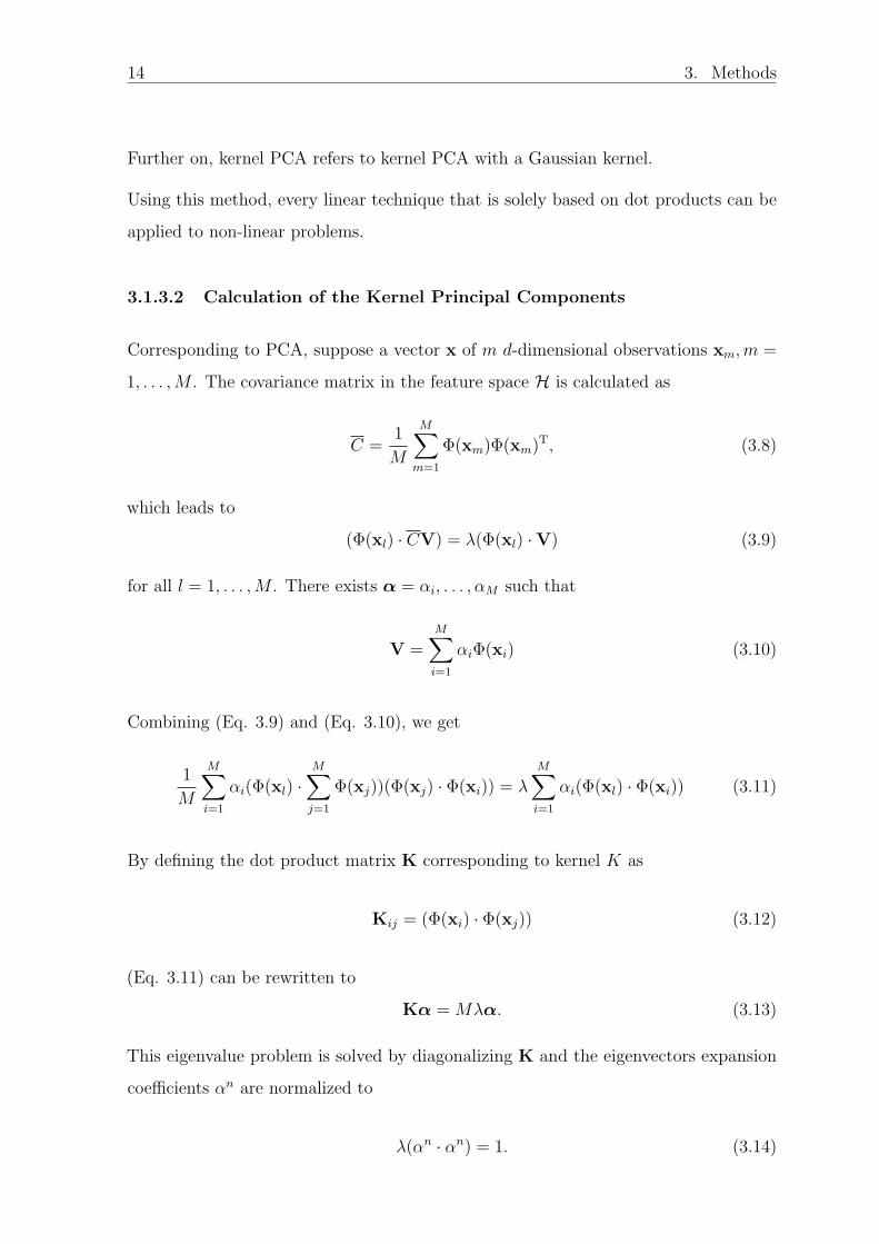
3.1.3.2 Calculation of the Kernel Principal Components

Corresponding to PCA, suppose a vector x of m d-dimensional observations xm, m =

1, . . . ,M . The covariance matrix in the feature space H is calculated as

C =1

M

M∑m=1

Φ(xm)Φ(xm)T, (3.8)

which leads to

(Φ(xl) · CV) = λ(Φ(xl) ·V) (3.9)

for all l = 1, . . . ,M . There exists α = αi, . . . , αM such that

V =M∑i=1

αiΦ(xi) (3.10)

Combining (Eq. 3.9) and (Eq. 3.10), we get

1

M

M∑i=1

αi(Φ(xl) ·M∑

j=1

Φ(xj))(Φ(xj) · Φ(xi)) = λM∑i=1

αi(Φ(xl) · Φ(xi)) (3.11)

By defining the dot product matrix K corresponding to kernel K as

Kij = (Φ(xi) · Φ(xj)) (3.12)

(Eq. 3.11) can be rewritten to

Kα = Mλα. (3.13)

This eigenvalue problem is solved by diagonalizing K and the eigenvectors expansion

coefficients αn are normalized to

λ(αn · αn) = 1. (3.14)

3.2. System comparison 15

Finally, to extract principal components corresponding to kernel K of point x the

projections onto the eigenvectors are computed by

(KPC)n(x) = (Vn · Φ(x)) =M∑i=1

αni (Φ(xi) · Φ(x)). (3.15)

3.1.4 Other nonlinear PCA methods

Hebbian Networks

By utilizing Oja’s Rule which was introduced by Oja (1982), artificial neural networks

(ANN) are able to compute principal components. When nonlinear activation functions

are used, nonlinear principal components are found.

These methods have advantages when the input data are not stationary, but lack a

geometric interpretation.

Deep Autoencoder

The deep autoencoder is a nonlinear generalization of PCA which uses an ANN with a

bottleneck. It is trained by using the input x as desired output y. As these networks

are big (typically with several hundred to thousand nodes and 5 to 11 fully connected

layers) it takes a long time to train.

Hinton and Salakhutdinov (2006) show that the deep autoencoder significantly outper-

formed PCA on the reconstruction error on a number of data sets.

In contrast to PCA and kernel PCA, these methods do not compute new bases, but

instead train ANNs. Comparing ANNs cannot be done with the methods to compare

bases and was beyond the scope of this work.

3.2 System comparison

The features extracted in the system representation step have to be compared to be

usable for deviation detection and clustering. In the case of PCA and Kernel PCA

16 3. Methods

these features are principal components, which span an orthogonal space. As not all of

the principal components are used, this space is further on referred to as subspace.

We thought about three methods to compare two subspaces: the angle between them,

the overlapping volume and the reconstruction error of the data with interchanged

subspaces.

The angle between two subspaces can be calculated as proposed by Krzanowski (1979).

The measure of similarity is the sum of the squared cosines of the angles between all

the eigenvectors. This measure is in the range of 0 (for non-overlapping spaces) to 1

(for coincident spaces) and symmetric, i.e. the similarity between the two subspaces A

and B is equal to the similarity between B and A.

The overlapping volume between two subspaces can be based on hyper-cuboid where

the side length are equal to the eigenvalues. This measure has the advantage of also

taking the eigenvalues into account. It is symmetric, but is not limited to a range of 0

to 1.

A similarity measure based on the reconstruction error with interchanged subspaces can

be calculated as follows: The principal components PCA and PCB are computed for

the two systems A and B respectively. The data of system A are transformed to the

new space span by PCA and the reconstruction error ENAA when using only the first N

principal components is calculated. Then the reconstruction error ENAB of transforming

the data of system A to the space span by first N principal components of PCB is

calculated. This similarity measure is neither symmetric, nor in the range of 0 to 1.

As the properties of the angle-based similarity measure are very convenient when

comparing different similarities, this measure is used further on. The successive methods

rely on these properties and thus, to use any of the other methods, each similarity

measure has to be rescaled to be in the range of 0 to 1. This, however, has to be done

in a way that the relationships between similarity measures of different systems are

represented correctly, i.e. pairs of systems with a similarity close to 1 are in fact more

similar than pairs with a lower similarity measure.

3.2. System comparison 17

3.2.1 Calculation of the Angle between two Subspaces

Suppose two subspaces L and M with N principal components. The matrices L =

(l1, . . . , ln) and M = (m1, . . . ,mn) contain these principal components as column

vectors.

The angle θ11 between their first principal components is calculated as

θ11 = arccos√〈l1, m1〉. (3.16)

of the two vectors l1 and m1. A measure of similarity can be defined as

s11 = cos2θ11 = 〈l1, m1〉. (3.17)

As shown by Krzanowski (1979), this can be generalized to more than one principal

component as

S(L, M) =1

N

N∑i=1

N∑j=1

cos2θij =1

Ntr LTMMTL. (3.18)

This similarity measure lies between 0 for non-overlapping spaces and 1 for coincident

spaces.

Wang et al. (2006) propose a subspace distance (SSD)

dwwf (L, M) =

√√√√N −N∑

i=1

N∑j=1

(lTi mj)2. (3.19)

Sun and Cheng (2006) show that dwwf(L, M) is a proper distance measure, i.e. it

satisfies the following properties:

• Non-negativity: 0 ≤ dwwf (L, M) for any L and M

• Symmetry: dwwf (L, M) = dwwf (M, L)

• Triangular inequality: dwwf (L, M) ≤ dwwf (L, Γ) + dwwf (Γ, M)

d2wwf (L, M) is proportional to S(L, M).

18 3. Methods

3.2.2 The Affinity Matrix

For more than two systems, the similarity measures (Eq. 3.18) between all subspaces

were combined into an affinity matrix A. For k systems with their d-dimensional

subspaces X1, ..., Xk, this affinity matrix is

A =

a11 a21 · · · ak1

a12 a22 · · · ak2...

.... . .

...a1k a2k . . . akk

(3.20)

whereai,j = S(Xi, Xj). (3.21)

This matrix is symmetric and the diagonal elements are 1.

Although we only use the angle based measure of similarity it is worth mentioning that

the affinity matrix can as well be based on any other similarity measure, as long as the

above mentioned properties apply.

The subsequent deviation detection and clustering methods are solely based on the affin-

ity matrix and, consequently, it effectively decouples them from the feature extraction

methods.

3.3 Deviation detection

The deviation detection is based on building a statistical model D of the affinities and

from this compute the probability of each observation given D.

We assume that the affinities from a given observation of a data set to all the other

observations follow a normal distribution. Although the affinity is limited (between

0 and 1) while the normal distribution extends to infinity, a small variance of the

affinities results in a narrow probability distribution function, where the significant

part lies between 0 and 1. For a reasonable data set this should hold. Otherwise

either the system representation step failed to produce a suitable representation, i.e.

a representation that preserves the relations between systems, or the systems are not

similar at all.

3.3. Deviation detection 19

The calculation of the probability to observe sample x given the data set S is done on

both, the mean affinities and on the separate affinities.

Calculation of P (x|S) based on the mean affinities:

1. Compute the affinity matrix A for {S, x} (i.e. the set of all samples from S andthe test sample x)

2. Compute the mean affinity a for every system in S, i.e. remove the diagonal andthen take the mean of every column

3. Let D ∼ N(µa, σ2a), where µa is the meanand σ2

a is the variance of all a

4. Calculate P (x|S) as the cumulative distribution function of D at ax

Calculation of P (x|S) based on the separate affinities:

1. Compute the affinity matrix A for {S, x}

2. For each system n of the N systems:

2.1. Take the affinities of all other systems to system n and store them in an

2.2. Let Dn ∼ N(µan, σ2an)

2.3. Calculate Pn = P (x|S) as the cumulative distribution function of Dn at axn

3. Calculate P (x|S) as the geometric mean N

√∏Nn=1 Pn

Both ways of calculating the probability P (x|S) use the means and variances of the

affinities. The mean and variance are sensitive to outliers. This shortcoming can

be overcome by using a technique to derive a robust estimate of P (x|S). One such

technique is bootstrapping.

(a) Mean affinities (b) Seperate affinities

Figure 3.3: The calculation of P (x|S) on the mean affinities and on the separate affinities

20 3. Methods

3.3.1 Bootstrapping

Bootstrapping is a statistical resampling method introduced by Efron (1979). By

random sampling with replacement it derives robust estimates of properties like mean

or median of the underlying distribution.

The bootstrapping algorithm to compute the probability of observing a system x given

data set S is as follows:

1. Take the set of measurements S of the size N and the system to test x.

2. Repeat M times

2.1. Pick a random bootstrap sample BS from S. The size n of this sample is0 < n < N

2.2. Compute the probability model for BS

2.3. Compute Pn(x|BS)

3. Estimate P (x|S) as the median of the set {P1(x|BS), . . . , PN(x|BS)}

0 2 4 6 8 100.4

0.5

0.6

0.7

0.8

0.9Mean affinities

System

(a) Mean affinities

0.4

0.5

0.6

0.7

0.8

0.9

0123

Probability Distribution

Density

(b) PD

0.4

0.5

0.6

0.7

0.8

0.9

051015

PD with Bootstrapping

Density

(c) PD with BS

Figure 3.4: The effect of bootstrapping on a synthetic data set with 20% outliers. (a)The mean affinities of a synthetic data set; (b) the probability distribution for the whole

dataset; (c) the probability distribution with bootstrapping (M = 20, n = 0.5)

3.4 Clustering

The goal of clustering is to group a data set into a number of groups, such that the

observations within one group are more similar to each other than to observations in

3.4. Clustering 21

other groups. The similarity between objects is calculated with a defined distance

measure. Common distance measures are Euclidean distance or Mahalanobis distance,

but also other measures can be used.

Clustering methods can be divided into two types: hierarchical and partitional clustering.

Hierarchical clustering methods produce the clusters of each level based on the clusters

of the previous level, while partitional clustering finds all clusters at once.

3.4.1 Spectral Clustering

Spectral clustering is a partitional clustering method. The idea of spectral clustering is

based on concepts from spectral graph theory, which studies the properties of graphs

with respect to the spectrum (i.e. the eigenvectors and eigenvalues) of its adjacency

and Laplacian matrix.

In graph theory the grouping of a graph into two disjoint sets is done by simply removing

the edges that connect the two sets and is called cut. The size of the cut is the sum

of the weights of all removed edges. Minimizing this cut value leads to the optimal

partition into two groups.

Shi and Malik (2000) introduce the normalized cut criterion to segment images and

show how this can be done by solving a eigenvalue system. This method uses an affinity

matrix that describes the similarity between any pair of nodes in the graph. In our

case, this affinity matrix is calculated as described in Sec. 3.2.2.

To segment the graph, the eigenvalue system has to be solved. Clustering into k groups

is then done by using k-means clustering on the eigenvectors.

Figure 3.5: Example of Spectral Clustering, the red lines show the cuts

22 3. Methods

3.4.2 Hierarchical Clustering

Hierarchical clustering builds up or breaks down a hierarchy of clusters. Building up a

hierarchy is called agglomerative hierarchical clustering, while breaking down is called

divisive hierarchical clustering.

Agglomerative clustering starts at the lowest level, where each cluster contains only

a single observation, and recursively reduces the number of clusters by merging the

two closest ones (bottom-up). Divisive clustering starts with one cluster that covers

the whole data set and recursively splits one cluster into two new clusters (top-down),

where the split is chosen in a way that the two new clusters have the largest possible

dissimilarity.

Hastie et al. (2001) state that divisive methods have potential advantages when aiming

to partition the data set into a small number of clusters.

Often the splitting is done by applying k-means or k-medoids clustering with K = 2,

but then of course such an approach depends on the starting configuration. An approach

that avoids this was invented by Macnaughton-Smith et al. (1964). It starts with a

single cluster G. The observation whose average dissimilarity to all other observations is

largest is removed from G and forms a new cluster H. At the next step the observation

with the largest average dissimilarity from H minus the average dissimilarity from G is

transferred to H. This is done until the largest value becomes negative, which means

that there are no more observations in G that are (on average) closer to H. This process

is visualized in Fig. 3.6.

Clustering into more than two clusters is done by recursively applying hierarchical

clustering on the resulting clusters.

This method is solely based on the measure of similarity and does not depend on any

(random) starting configuration.

3.4. Clustering 23

Figure 3.6: Hierarchical clustering with the Macnaughton-Smith approach of cluster Ginto clusters G and H. The red systems belong to cluster G and the blue ones to H.

4

Data sets

We wanted to test our approach on two different types of mechatronical systems. Hence

we used

• data of a simulated vehicle cooling system

• human gait data.

The cooling system data is also analyzed in Byttner et al. (2008).

We use the human gait pattern to illustrate a possible humanoid robot.

4.1 Vehicle Cooling System

The cooling system data is provided by a vehicle manufacturer and is generated with a

simulation model of a cooling system.

Every simulation has at least 1600 consecutive observations with 51 signals such as fan

speed, cooling water and oil temperature, engine speed and other parameters that are

considered relevant for the cooling system.

Two data sets that simulate different failures are available. Both sets contain a number

of reference systems without any failure and systems with failures at different severity

levels. The systems are from one of three different weight classes (15 tons, 18 tons and

23 tons) and three different ambient temperatures (10◦C, 20◦C and 30◦C).

25

26 4. Data sets

4.1.1 Healthy Systems

The leakage data set contains 9 healthy systems, one from each weight class and ambient

temperature. These systems are denoted by their weight and temperature, e.g. 15t10.

The data set of the soiled model contains another three healthy systems for each weight

class at a constant ambient temperature of 20◦C. Further on, these systems are denoted

by the suffix s0 e.g. 15t20 s0.

Together, these 12 systems form the “normal” data set.

4.1.2 Systems with a Leakage

This data set was generated with a model that simulates a leakage in the cooling system.

The model has a certain amount of air added to the coolant mixture, which lowers its

heat capacity.

There are three different severity levels, 20%, 40% and 60% air for each of the weight

class and ambient temperature, making a total of 27 leakage systems.

Systems with a leakage are labeled with a suffix like l20.

4.1.3 Soiled Systems

The model used for this data set simulates a cooling system with a soiled radiator. A

given fraction of the radiators surface is covered with dirt, lowering its ability to emit

heat and therewith the cooling efficiency.

Again, there are three different levels of severity, 15%, 30% and 50% of the surface for

each of the three weight classes at an ambient temperature of 20◦C.

Soiled systems are denoted with a suffix like s15.

4.2 Human Gait Data

Two different motion capturing data sets were used. Unfortunately their formats are

incompatible and therefore they had to be examined separately.

4.2. Human Gait Data 27

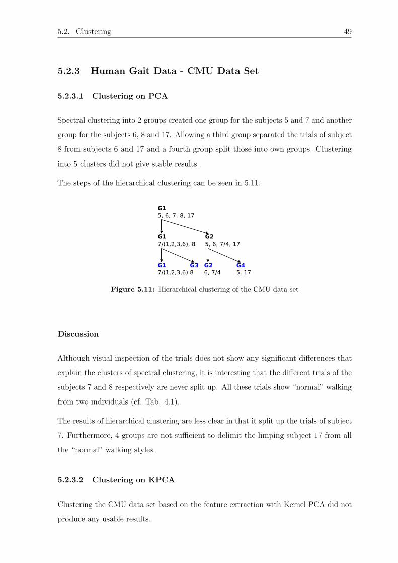
4.2.1 CMU Data Set

This data set was obtained from the CMU Graphics Lab Motion Capture Database

in Acclaim Motion Capture (AMC) format. These files contain 62 features that are

captured at a frame rate of 120 frames per second.

12 samples for “normal” walking and one “faulty”, limping samples from five different

subjects were picked. After visual inspection they were trimmed to 300 frames and

the toe and hand features1 and the absolute position in the world frame were removed.

Tab. 4.1 shows the used subjects and trials.

Style Subject Trial

“normal” walking 5 16 17 1, 2, 3, 4, 68 2, 3, 4, 7, 11

limping 17 5

Table 4.1: CMU Data Set subjects and trials

−1200−1000

−800−600

8001000

12001400

16001800

20002200

24002600

200

400

600

800

1000

1200

1400

x

Skeleton of the CMU data set

z

y

Figure 4.1: Example skeleton of the CMU data set

1CMU Graphics Lab states that these features tend to be noisy and visual inspection confirmedthis.

28 4. Data sets

4.2.2 MIT Data Set

The MIT data set was used by Hsu et al. (2005). It contains various different walking

styles: normal walking, jogging, waddling, swaying, walking sideways and limping.

Three different speeds are available for each style, slow, medium and fast that vary in

step size.

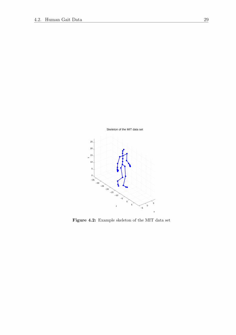
The format used for these data does not divide the information into a skeleton that

defines the connections and distances between joins and the motion data that states

the angles for each joint at a time. Instead it gives angles and distance in x, y and

z direction with respect to its parent joint. As the offsets are only dependent on the

person, but not on the walking style, they were removed.

Visual inspection revealed that the sections featuring the specific walking style were

interrupted by sections of normal walking. Hence, it was necessary to extract continuous

sections of the specific walking style, which all show walking on a straight line and are

300 frames long.

Sample Style Speed

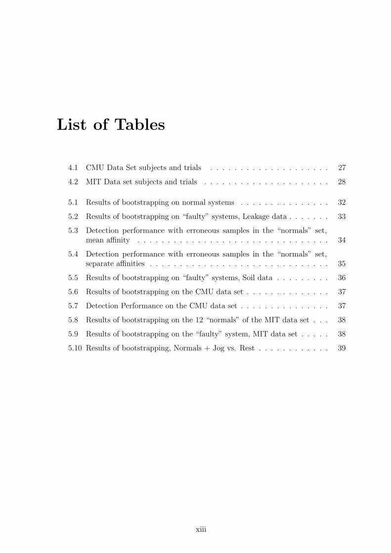
1 - 4 Normal Slow5 - 8 Normal Medium9 - 12 Normal Fast

13 Jog Slow14 Jog Medium15 Waddle Fast16 Sway Medium17 SideRight Slow18 SideRight Medium19 SideRight Fast20 Limp Slow21 Limp Medium22 Limp Fast

Table 4.2: MIT Data set subjects and trials

4.2. Human Gait Data 29

−50

5

−35

−30

−25

−20

−15

−10

−5

0

5

0

5

10

15

20

25

x

Skeleton of the MIT data set

z

y

Figure 4.2: Example skeleton of the MIT data set

5

Results and Discussions

5.1 Deviation detection

This section presents the results of the deviation detection method on the four data

sets. Observations that have a likelihood below 5% are considered as deviating.

Throughout this section the data sets are split into their naturally distinct parts of

“normal” and “faulty” systems.

5.1.1 Cooling System with a Leakage

5.1.1.1 Deviation Detection based on PCA

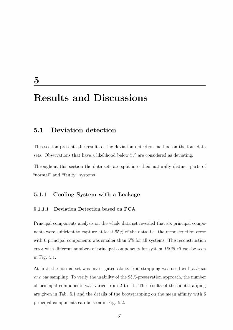
Principal components analysis on the whole data set revealed that six principal compo-

nents were sufficient to capture at least 95% of the data, i.e. the reconstruction error

with 6 principal components was smaller than 5% for all systems. The reconstruction

error with different numbers of principal components for system 15t20 s0 can be seen

in Fig. 5.1.

At first, the normal set was investigated alone. Bootstrapping was used with a leave

one out sampling. To verify the usability of the 95%-preservation approach, the number

of principal components was varied from 2 to 11. The results of the bootstrapping

are given in Tab. 5.1 and the details of the bootstrapping on the mean affinity with 6

principal components can be seen in Fig. 5.2.

31

32 5. Results and Discussions

0 2 4 6 8 100

5

10

15

20

25

30

35

40

45

50Reconstruction Error against Principal Components

Principal Components

Rec

onst

ruct

ion

Err

or [%

]

Figure 5.1: Reconstruction Error against Principal Components for System 15t20 s0

Number of PC Deviating Systems Deviating System(mean affinity) (affinity)

2 No deviation No deviation3 15t30 No deviation4 15t10 15t105 23t30 No deviation6 18t30 18t30

7 - 11 18t30 18t30

Table 5.1: Results of bootstrapping on normal systems

The deviation detection was then carried out with bootstrapping on the mean affinity

and on the separate affinities in a one versus all fashion, i.e. one “faulty” system was

compared to all “normal” systems. Again the number of principal components was

varied from 2 to 11 to evaluate their influence on the detection performance. Tab. 5.2

shows the number of detected deviations out of the 27 “faulty” systems.

Discussion

As Tab. 5.1 shows, with six and more principal components system 18t30 was con-

sistently detected as deviating. It was, however, impossible to check if there were

any errors in the simulation and system 18t30 was therefore not removed from the


0 2 4 6 8 10 120.8

0.81

0.82

0.83

0.84

0.85

0.86

0.87

0.88

0.89

0.9Mean affinities for the Normal Systems

System

Mea

n af

finity

(a) Mean affinities

0 2 4 6 8 10 120

0.1

0.2

0.3

0.4

0.5

0.6

0.7

0.8Probability for being Normal

System

Pro

babi

lity

(b) Probabilities

Figure 5.2: (a) The mean affinities within the group of normal systems (b) the proba-bilities calculated with bootstrapping and leave-one-out sampling on the mean affinities

Number of PC Deviating Systems Deviating Systems(mean affinity) (affinity)

2 5 53 13 144 8 85 19 36 27 27

7 - 11 27 27

Table 5.2: Number of systems detected as deviations out of 27 “faulty” leakage datasamples

“normals”.

Tab. 5.2 shows that with six and more principal components it was also possible to

detect all 27 “faulty” systems as deviations from the “normal” set when the “normal”

set includes system 18t30.

These results clearly indicate that the approach works on this data set.

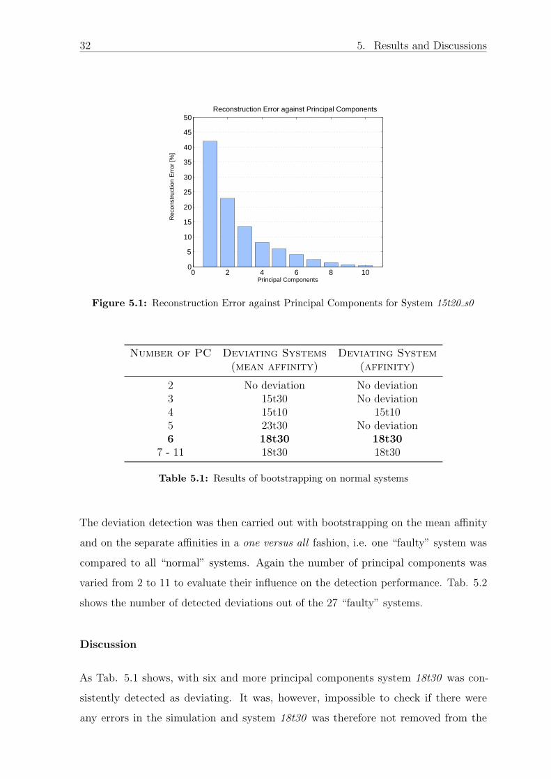
5.1.1.2 Detection Performance with Erroneous Normals

To evaluate the stability of the detection performance against “faulty” systems within

the group of “normals”, 0 - 4 random faulty systems were added to the set of normals.

Deviation detection was then done 100 times and the detection performance was


Erroneous Test Detected DeviationsSamples Samples Mean Std.Dev Min Max

0 27 27 0 27 271 26 20.4 6.7 3 262 25 10.4 4.6 2 183 24 5.0 2.3 2 124 23 3.6 1.6 2 9

Table 5.3: Detection performance with erroneous samples in the “normals” set, boot-strapping on mean affinities with 6 principal components

0 1 2 3 40

20

40

60

80

100

Detection Performance with Erroneous Samples

Number of Erroneous Samples

Det

ectio

n P

erfo

rman

ce [%

]

Figure 5.3: Detection rate with erroneous samples in the “normals” set, bootstrappingon mean affinities with 6 principal components

measured. The results for deviation detection using the mean affinity are given in Tab.

5.3 and Fig. 5.3 and those for deviation detection using the separate affinities are given

in Tab. 5.4.

It is worth noting for this set of experiments the group of “normals” already contained

a possibly “faulty” system, namely 18t30.

Discussion

Assuming that system 18t30 is erroneous, the “normals” already contain 8% erroneous

samples. By adding 4 more erroneous samples to this set, more than 30% of the


Erroneous Test Detected DeviationsSamples Samples Mean Std.Dev Min Max

0 27 27 0 27 271 26 18.1 4.1 2 242 25 4.4 1.7 1 83 24 2.1 0.4 1 54 23 1.8 0.6 0 5

Table 5.4: Detection performance with erroneous samples in the “normals” set, boot-strapping on separate affinities with 6 principal components

“normals” are faulty. It is comprehensible that a deviation detection does not perform

well under this conditions.

5.1.1.3 Deviation Detection based on Kernel PCA

Using bootstrapping on the outcome of Kernel PCA feature extraction did not give

usable results. Even though bootstrapping with mean affinities flagged some systems

as outliers the detected systems varied and, thus, we assume that these detections are

highly dependent on the random composition of the bootstrap sample.

This is caused by the fact that the affinities between systems of different weight classes

are very low (i.e. they are very dissimilar, see Fig. 5.8 a in Sec. 5.2.1.3) and so for each

system, more than 23

of all the other systems are very dissimilar.

5.1.2 Soiled Cooling System

As described in Sec. 4, the “normal” systems for the soil data set were the same as for

the leakage data set, while the “faulty” set was made up by 9 soiled systems instead of

27 systems with a leakage.

PCA revealed that six principal components were again sufficient for the “faulty”

systems of this data set and thus the trials from the previous section were repeated.

Applying bootstrapping did not result in any stable detections when using fewer than six

principal components. Three deviating systems were detected when using six or more



2 0 03 2 2

4 , 5 0 06 3 3

7 - 11 3 3

Table 5.5: Number of systems detected as deviations out of 9 “faulty” soil data samples

principal components. These three systems were 18t20 s50, 23t20 s30 and 23t20 s50.

Tab. 5.5 shows the number of detected deviations out of the 9 “faulty” systems.

Discussion

A soiled radiator does not effect the cooling system as severely as a leakage does.

Consequently, it is understandable that a soiled system is harder to detect than a

system with leakage. This is also reflected by the detection performance of this data

set.

The three detected systems 18t20 s50, 23t20 s30 and 23t20 s50 are those that one

would most likely expect to be affected by soil in the cooling system, as these are the

heavy ones with a high soil level.

5.1.3 Human Gait Data - CMU Data Set

This data set contained 12 trials of “normal” walking from four different subjects and

one trial of limping from yet another subject. It required 13 principal components to

describe 95% of the variance of the original data. As for the vehicle cooling system

data sets, different numbers of principal components were tried out. In this case the

number was varied from 8 to 18 (13± 5).

First of all, the whole data set was inspected with bootstrapping on the mean affinity

as well as on the separate affinities. The results are in Tab. 5.6.



8 5/1, 17/5 8/49, 10 5/1, 17/5 No deviation11 5/1, 17/5 17/5

12-18 17/5 17/5

Table 5.6: Results of bootstrapping on the CMU data set


8-10 1 010-18 1 1

Table 5.7: Detection Performance on the CMU data set

Subsequently a one versus all test was done too with both deviation detection methods.

Tab. 5.7 shows that 8 principal components were sufficient to detect the limping

individual with bootstrapping on the mean affinity. Bootstrapping on the separate

affinities worked with 10 and more principal components.

Discussion

The inspection of the whole data set showed that bootstrapping on the mean affinity

as well as on the separate affinities was able to detect the limping individual with 12

and more principal components. Obviously, the 8 features were already sufficient to

describe the difference of trial 17/5 from the others but 12 features were necessary to

cover the similarity of trial 5/1 to the others.

5.1.4 Human Gait Data - MIT Data Set

From the 54 features that were captured for the MIT data set PCA produced 10 which

were sufficient for the 95% approach. However, 5 - 15 principal components were used

for the experiments.


Number of PC Deviating System Deviating System(mean affinity) (affinity)

5 - 7 No deviation No deviation8, 9 Normal Slow 4 Normals Slow 4

10 - 12 No deviation No deviation13 - 15 Normal Slow 1 No deviation

Table 5.8: Results of bootstrapping on the 12 “normals” of the MIT data set


5-15 10 10

Table 5.9: Detection Performance

The inspection of the “normal” walking styles did not reveal any outstandingly deviating

sample, although the samples Slow 4 and Slow 1 were detected as outliers with some

numbers of principal components. Tab. 5.8 gives all results.

During the subsequent deviation detection, where one of the “other” samples was

compared to the 12 “normals”, all 10 “others” were detected as deviating with any

number of principal components, see Tab. 5.9. The affinity matrix shown in Fig. 5.4

illustrates the reason for this.

To have more variations in the systems that are considered “healthy”, the two jog

samples were added to the normals. The deviation detection was then redone using

this enlarged set of healthy systems as reference. The samples featuring waddling and

swaying styles were not detected as deviations in this experiment, while most of the

samples showing walking sideways and limping were detected. The detailed results are

given by Tab. 5.10.

Discussion

The fact that none of the “normals” is detected as outlier is not very surprising as all

the samples show the same individual and essentially only differ in walking speed.


5

10

15

20

5 10 15 20

Affinity Matrix of the MIT Data set − 1 PC

0.4

0.5

0.6

0.7

0.8

0.9

1

(a) Affinity matrix with 1 principalcomponent

5

10

15

20

5 10 15 20

Affinity Matrix of the MIT Data set − 10 PC

0.4

0.5

0.6

0.7

0.8

0.9

1

(b) Affinity matrix with 10 principalcomponents

Figure 5.4: Affinity matrices of the MIT data set, 1 and 10 principal components


5 - 8 SideRight, Limp SideRight, Limp9 SideRight, Limp SideRight, Limp

Medium and Fast10 SideRight, Limp SideRight Medium and

Fast, Limp Fast11 SideRight, Limp SideRight, Limp Medium12 SideRight, Limp SideRight, Limp Slow13 SideRight, Limp SideRight Medium and

Fast, Limp Medium14 SideRight, Limp SideRight

Medium and Fast15 SideRight SideRight

Table 5.10: Results of bootstrapping, Normals + Jog vs. Rest

The affinity matrices in Fig. 5.4 perfectly show the reason for the good results of the

deviation detection. The affinities within the “normal” samples are very high compared

to the other affinities.

The results of the enlarged set of healthy systems make perfect sense, as walking

sideways is odder than limping. However, both are odder than jogging and therefore

detected as deviations, while waddling and swaying are closer to normal.


5.2 Clustering

5.2.1 Cooling System with a Leakage

5.2.1.1 Spectral Clustering on PCA

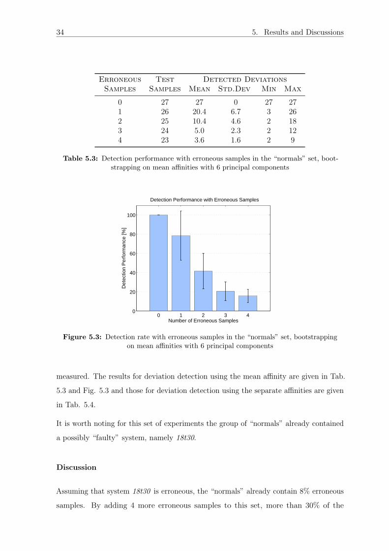
Like the deviation detection, the clustering was based on the affinity matrix. The number

of principal components used to calculate the affinity matrix was again determined

with the 95% preservation approach. Fig. 5.5 a shows a graphical representation of the

affinity matrix for the leakage data set.

Spectral clustering was done with the normalized cut partitioning algorithm, which uses

the k-means algorithm. The cluster centers were initialized randomly, which influenced

the outcome. The clustering was therefore repeated 100 times. The result was a matrix

with the probabilities that systems were grouped together. Such matrices are shown in

Fig. 5.6 a-c.

To find usable numbers of clusters the clustering was done for 2 - 10 clusters and the

number of groupings > 90% was observed. Groupings > 90% indicated that the related

systems were consistently grouped together and are not dependent on the random

initialization. As the number of groupings varied, this experiment was repeated 15

times. Additionally the clustering was performed on random affinity matrices. These

random affinity matrices were constructed such that they had the same properties as

real affinity matrices, i.e. they were symmetric with ones on the diagonal. The result

can be seen in Fig. 5.5 b.

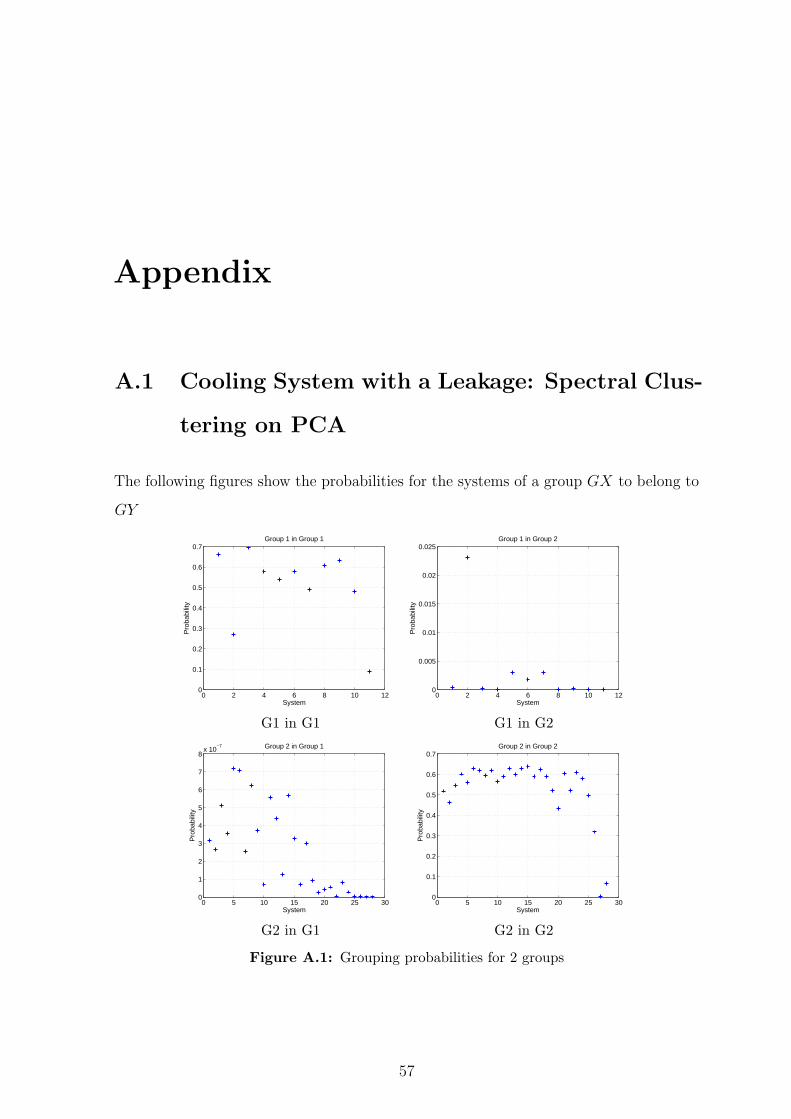
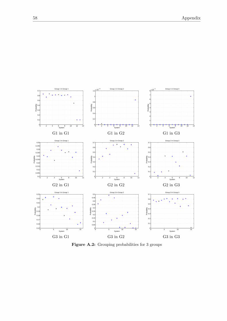
Additionally, for every clustering the probability for each system to belong to the cluster

where its assigned to and to belong to the other cluster(s) is calculated. This probability

is calculated as the normal cumulative distribution function for the mean affinity of a

certain system in the cluster given the cluster.

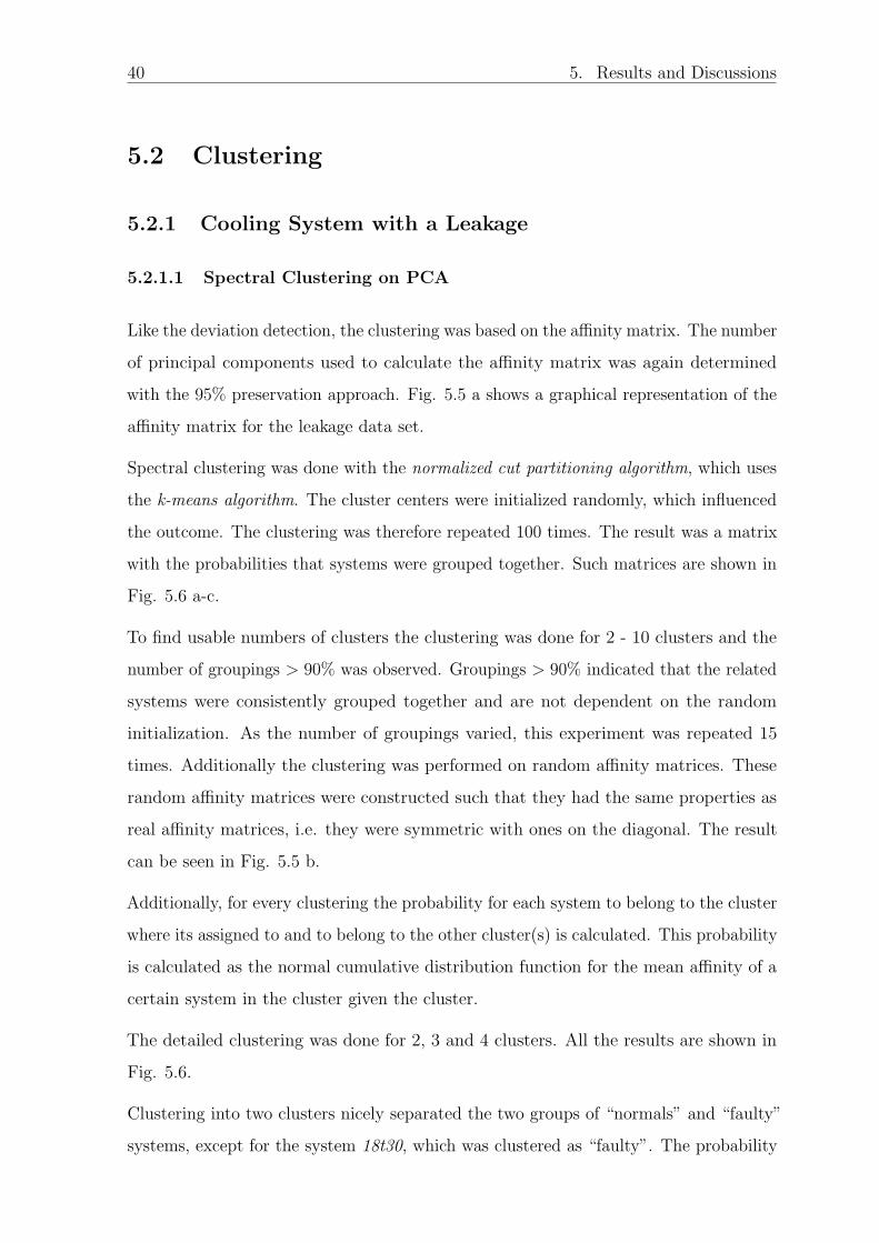
The detailed clustering was done for 2, 3 and 4 clusters. All the results are shown in

Fig. 5.6.

Clustering into two clusters nicely separated the two groups of “normals” and “faulty”

systems, except for the system 18t30, which was clustered as “faulty”. The probability

5.2. Clustering 41

5

10

15

20

25

30

35

5 10 15 20 25 30 35

Affinity Matrix of Leakage data

0.8

0.85

0.9

0.95

1

(a) Affinity Matrix

2 4 6 8 100

50

100

150

200

250

300

350

400

450

500

Clusters

Gro

upin

gs >

90%

Groupings against Number of Clusters

(b) Groupings against the number of clusters

Figure 5.5: (a) The affinity matrix of the Leakage data set (b) Number of systemsgrouped together in at least 90 out of 100 cases. Blue is for 15 spectral clusterings on the

affinity matrix in (a), red is for 15 random affinity matrices

for any system of the “normals” cluster to actually belong to the “faulty” cluster was

below 3% and the probability for any “faulty” system to belong to the “normals” cluster

was even lower.

The result for 3 clusters gave the following groupings:

Group 1 The “normals” and the two worst systems

15t10, 15t20, 15t20 s0, 15t30, 18t10, 18t20, 18t20 s0, 23t10, 23t20, 23t20 s0,

23t30, 23t20 l60 and 23t30 l60

Group 2 The “faulty” systems 1: lighter, cooler, smaller degree of leakage + 18t30

18t30, 15t10 l20, 15t20 l20, 15t30 l20, 18t10 l20, 18t20 l20, 23t10 l20, 15t10 l40,

15t20 l40, 18t10 l40 and 15t10 l60

Group 3 The “faulty” systems 2: heavier, warmer, bigger degree of leakage

18t30 l20, 23t20 l20, 23t30 l20, 15t30 l40, 18t20 l40, 18t30 l40, 23t10 l40, 23t20-

l40, 23t30 l40, 15t20 l60, 15t30 l60, 18t10 l60, 18t20 l60, 18t30 l60 and 23t10 l60

Clustering into 4 clusters gave essentially the same result, but formed an extra cluster

for the two worst systems so that group 1 contained only “normal” systems.

The figures that show all the probabilities can be found in the appendix.


5

10

15

20

25

30

35

5 10 15 20 25 30 35

Spectral Clustering − 2 Clusters

(a) 2 clusters

5

10

15

20

25

30

35

5 10 15 20 25 30 35


(b) 3 clusters

5

10

15

20

25

30

35

5 10 15 20 25 30 35


(c) 4 clusters

5

10

15

20

25

30

35

5 10 15 20 25 30 35


(d)

5

10

15

20

25

30

35

5 10 15 20 25 30 35


(e)

5

10

15

20

25

30

35

5 10 15 20 25 30 35


(f)

5

10

15

20

25

30

35

5 10 15 20 25 30 35


(g)

5

10

15

20

25

30

35

5 10 15 20 25 30 35


(h)

5

10

15

20

25

30

35

5 10 15 20 25 30 35


(i)

Figure 5.6: Results of spectral clustering on the PCA of the leakage data set. (a-c)show the outcome of 100 spectral clusterings into 2, 3 and 4 clusters. (d-f) show these

results for the actual allocations and (g-i) show them after sorting

5.2. Clustering 43

Discussion

The fact that system 18t30 is grouped together with the “faulty” systems is perfectly

consistent with the findings of the deviation detection.

The reason that the two worst systems are grouped together with the “normals”, while

the the other “faulty” systems are grouped into two clusters is most likely that they are

so few and thus the optimal normalized cut separates the big group of faulty systems

into two smaller ones.

5.2.1.2 Hierarchical Clustering on PCA

The hierarchical clustering algorithm described in Sec. 3.4.2 separates a given group

into two clusters and is solely based on a measure of similarity like the affinity matrix.

The first group G1 to cluster is the whole data set.

The following systems are moved to the second cluster G2 in the given order: 23t30,

23t20 l60, 23t20, 15t30, 23t20 s0, 23t10, 15t20, 15t20 s0, 18t10, 18t20, 18t20 s0,

15t10 and 23t30 s60.

Further splitting of G2 separated the two worst from the “normal” systems, while

further splitting of G1 separated 15t10 l20, 15t10 l60 and 23t10 l60 from the other

“faulty” systems. The splitting into 3 groups is visualised in Fig. 5.7.

Figure 5.7: Hierarchical clustering into 3 groups


Discussion

It is interesting that the systems in group G2 after the first clustering are the same

systems as group 1 from the spectral clustering into 3 clusters.

The clustering into the 3 groups as illustrated in Fig. 5.7 is the clearest grouping.

5.2.1.3 Clustering on KPCA

For the KPCA the approach of preserving 95% of the variance of the data was not

usable, because it is not possible to reconstruct the extracted features in the input

space and calculate the error.

However, as shown in Scholkopf et al. (1998), the KPCA is calculated as a kernel

eigenvalue problem. These eigenvalues are sorted and divided by the sum of all

eigenvalues up to the dimension of the original data. This value was then used as an

estimate of the contribution of this eigenvalue. As many of the features were used so

that the estimated contribution exceeded 95%.

For the systems in the leakage data set this required between 2 and 5 features, so 5

features were used. Using fewer features decreased the performance by steadily assigning

the “under-described” systems to wrong groups.

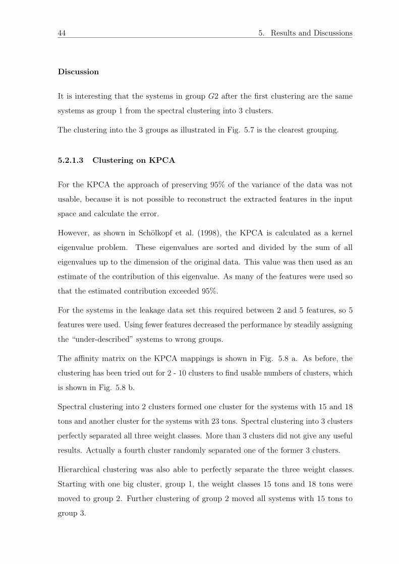
The affinity matrix on the KPCA mappings is shown in Fig. 5.8 a. As before, the

clustering has been tried out for 2 - 10 clusters to find usable numbers of clusters, which

is shown in Fig. 5.8 b.

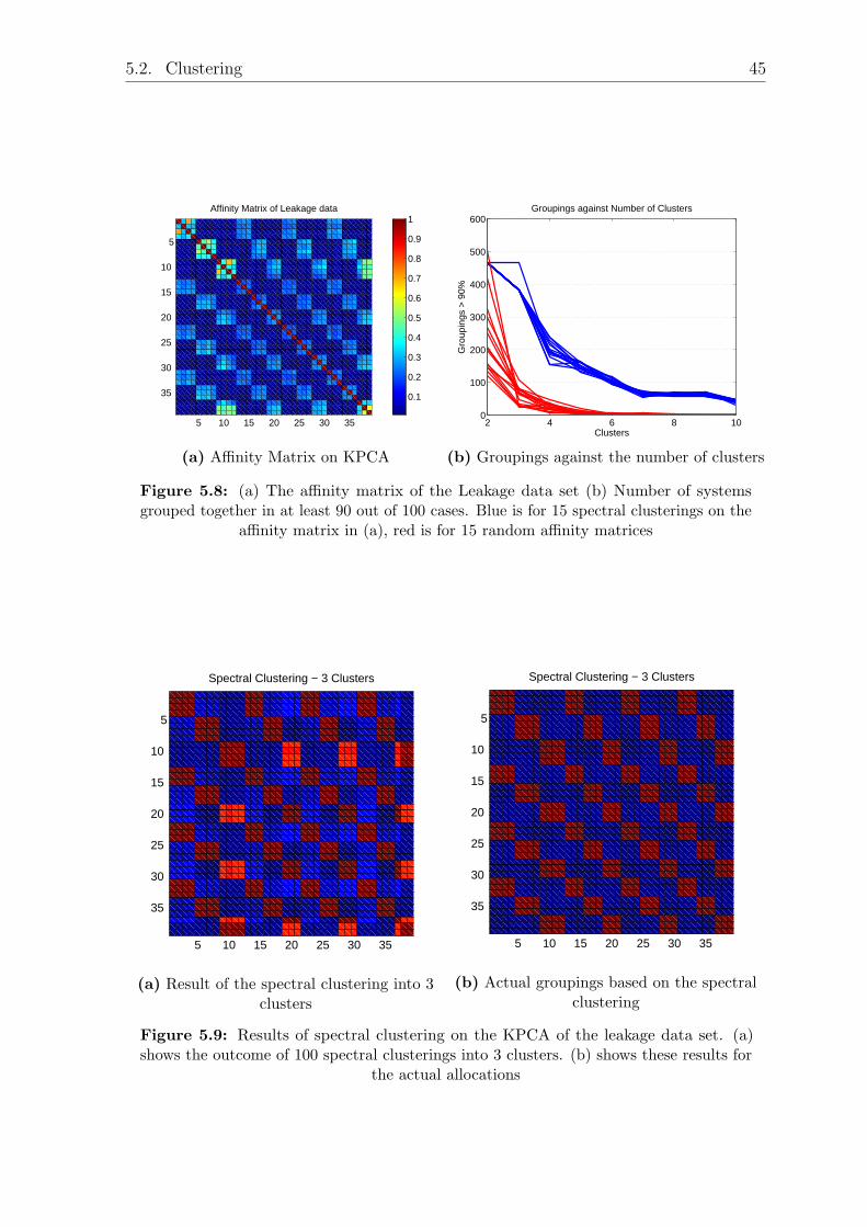
Spectral clustering into 2 clusters formed one cluster for the systems with 15 and 18

tons and another cluster for the systems with 23 tons. Spectral clustering into 3 clusters

perfectly separated all three weight classes. More than 3 clusters did not give any useful

results. Actually a fourth cluster randomly separated one of the former 3 clusters.

Hierarchical clustering was also able to perfectly separate the three weight classes.

Starting with one big cluster, group 1, the weight classes 15 tons and 18 tons were

moved to group 2. Further clustering of group 2 moved all systems with 15 tons to

group 3.

5.2. Clustering 45

5

10

15

20

25

30

35

5 10 15 20 25 30 35

Affinity Matrix of Leakage data

0.1

0.2

0.3

0.4

0.5

0.6

0.7

0.8

0.9

1

(a) Affinity Matrix on KPCA

2 4 6 8 100

100

200

300

400

500

600

Clusters

Gro

upin

gs >

90%

Groupings against Number of Clusters

(b) Groupings against the number of clusters

Figure 5.8: (a) The affinity matrix of the Leakage data set (b) Number of systemsgrouped together in at least 90 out of 100 cases. Blue is for 15 spectral clusterings on the

affinity matrix in (a), red is for 15 random affinity matrices

5

10

15

20

25

30

35

5 10 15 20 25 30 35


(a) Result of the spectral clustering into 3clusters

5

10

15

20

25

30

35

5 10 15 20 25 30 35


(b) Actual groupings based on the spectralclustering

Figure 5.9: Results of spectral clustering on the KPCA of the leakage data set. (a)shows the outcome of 100 spectral clusterings into 3 clusters. (b) shows these results for

the actual allocations


Clustering within one of these three groups separated the systems with small and medium

leakage size from those without leakage and with big leakage size. Any additional step

failed to separate these groups according to the leakage size.

Discussion

Considering the affinity matrix from Fig. 5.8 a the results are not surprising. The

affinity matrix already shows the three clusters very clearly.

Also it can be expected from the previous sections that the results of hierarchical

clustering are comparable to those from spectral clustering.

5.2.2 Soiled Cooling System

5.2.2.1 Clustering on PCA

Spectral clustering into 2 clusters gave the following groupings:

Group 1 The “cooler” systems - lower weight, ambient temperature and soil level

15t10, 15t20, 15t20 s0, 15t30, 18t10, 18t20, 18t20 s0, 23t10, 23t20 s0, 15t20 s15,

15t20 s30 and 18t20 s15

Group 2 The “warmer” systems - higher weights, ambient temperatures and soil level

18t30, 23t20, 23t30, 15t20 s50, 18t20 s30, 18t20 s50, 23t20 s15, 23t20- s30

and 23t20 s50

Spectral clustering into 3 clusters formed one group for the “cooler” systems that only

contained healthy systems.

Group 1 The “cool” systems

15t10, 15t20, 15t20 s0, 15t30, 18t10, 23t10 and 23t30

Group 2 The “medium” systems

18t20, 18t20 s0, 23t20, 23t20 s0, 15t20 s15, 15t20 s30, 15t20 s50, 18t20-

s15, 18t20 s30 and 23t20 s15

5.2. Clustering 47

Group 3 The “warm” systems

18t30, 18t20 s50, 23t20 s30 and 23t20 s50

Spectral clustering into 4 clusters gave the following groupings:

Group 1 Healthy and cool

15t10, 15t20, 15t20 s0, 15t30, 18t10 and 23t10

Group 2 Mixed 1

18t20, 18t20 s0, 23t20 s0, 15t20 s30 and 18t20 s15

Group 3 Mixed 2

23t20, 23t30, 15t20 s15, 15t20 s50, 18t20 s30 and 23t20 s15

Group 4 Faulty and warm

18t30, 18t20 s50, 23t20 s30 and 23t20 s50

Discussion

Clustering into two clusters separates the systems with lower weight, ambient temper-

ature and soil degree from those with higher weight, ambient temperature and soil

degree. The soiled systems in the first cluster are the ones that one would expect to be

least effected by the soiled radiator, 15 tons with low and medium soil degree and 18

tons with low soil degree.

Clustering into three clusters formed one group for the “cooler” systems that only

contains healthy systems and a “warm” group with only faulty systems and system

18t30. The “medium” group contains the warmer healthy systems and the cooler faulty

systems.

The clustering into four clusters gave almost the same result. The warmest system of

the previous “cooler” group, 23t30, was no longer situated in the “healthy and cool”

group. The previous “medium” group was split into two mixed groups, which contain

both “healthy” and “faulty” systems. The last group “faulty and warm“ was identical

to the previous “warm” group.



As the two cooling system data sets are very similar, the results of clustering each data

set are similar, too. Thus, it is not surprising that KPCA gave features that separated

the soiled cooling system data into weight classes.

Alike for the cooling system with a leakage, spectral clustering into 2 clusters separated

the systems with 23 tons from those with 15 and 18 tons. Clustering into 3 clusters

perfectly separated all 3 weight classes. The fourth cluster separated the system 18t30

from the 18 tons cluster.

Hierarchical clustering on the other hand moved the 15 and 23 tons systems from

the initial group G1 to the new group G2. Clustering this group G2 separated the

two weight classes, but system 23t10 was grouped together with the 15 tons systems.

Splitting the remaining group G1 separated 18t30 from the other 18 tons systems.

Figure 5.10: Hierarchical Clustering of the Soiled Cooling System. The * is used as awild-card for all possible systems matching the given expression.

Discussion

The findings of this section are similar to those of clustering on KPCA of the cooling

system with leakage.

5.2. Clustering 49

5.2.3 Human Gait Data - CMU Data Set


Spectral clustering into 2 groups created one group for the subjects 5 and 7 and another

group for the subjects 6, 8 and 17. Allowing a third group separated the trials of subject

8 from subjects 6 and 17 and a fourth group split those into own groups. Clustering

into 5 clusters did not give stable results.

The steps of the hierarchical clustering can be seen in 5.11.

Figure 5.11: Hierarchical clustering of the CMU data set

Discussion

Although visual inspection of the trials does not show any significant differences that

explain the clusters of spectral clustering, it is interesting that the different trials of the

subjects 7 and 8 respectively are never split up. All these trials show “normal” walking

from two individuals (cf. Tab. 4.1).

The results of hierarchical clustering are less clear in that it split up the trials of subject

7. Furthermore, 4 groups are not sufficient to delimit the limping subject 17 from all

the “normal” walking styles.


Clustering the CMU data set based on the feature extraction with Kernel PCA did not

produce any usable results.


A detailed investigation revealed that the affinities between all systems were very low.

Another way of calculating the affinity between two representations might overcome

this problem.

5.2.4 Human Gait Data - MIT Data Set


Spectral clustering into 2 clusters divided the samples of walking sideways and limping

from the other styles. Clustering into 3 clusters formed one cluster for normal walking,

one for walking sideways and another one of waddling, swaying, jogging and limping.

Clustering into 4 or more clusters did not result in reasonable separations.

Hierarchical clustering found the clusters shown in Fig. 5.12

Figure 5.12: Hierarchical clustering of the MIT data set

Discussion

The groupings found on this data set can be easily explained by the assumption that

from all the walking styles, walking sideways is the most odd one, followed by jogging

and limping. Although not perfectly normal, but still following the same motion

pattern, swaying and waddling are closest to the samples of normal walking. This is

also consistent with the findings of the deviation detection on this data set.

6

Summary and Conclusion

The proposed approach provides the ability to efficiently describe large amounts of data

with a compressed representation, compare such compressed representations and finally

detect deviations among groups of systems based on these compressed representations.

The compressed representation is needed to

• reduce the amount of data to transfer.

This allows transmission of data over low bandwidth media such as radio commu-

nication, which is important in environments with many mechatronical systems.

• reduce requirements of storage space and processing time and facilitates handling

of large amounts of systems.

Hence the scalability of the proposed approach is significantly improved.

The second step, comparing compressed representations, computes measures of similarity

between systems and combines them in a so-called affinity matrix. The successive

computations are exclusively based on this measure. Consequently, this step decouples

the representation from the deviation detection. As a result, additional representation

methods can be added without the need to adapt the deviation detection methods as

well as vice versa.

In the proposed approach, the final deviation detection is done in two different ways:

• the probability for each system to be observed given all the other systems is

calculated. Systems with a probability below a certain threshold, e.g. 5%, are

flagged as deviating.

51

52 6. Summary and Conclusion

• all systems are clustered. Systems with similar features are hereby clustered

together. In a population where most of the systems are “healthy” (such that

they appear to be similar using a certain representation) the deviating systems

form one or more smaller clusters.

These two methods can also be combined. For example, the clustering can be done

using one compressed representation and subsequently the probabilities for each system

to be “normal” within a cluster can be calculated using another representation. It

might have been a very successful approach for the soiled cooling system data set to

first cluster it using KPCA and then calculate the probabilities based on PCA, but was

omitted due to the size of the data set.

Using the proposed approach to analyze four data sets from two different domains,

a simulated cooling system and human gait data, demonstrates it applicability to

simulated data with systems from well separated classes as well as real world data.

In contrast to the method from Byttner et al. (2008), the proposed approach is not

only able to detect vehicles with a leakage level of 60%, but any vehicle with a leakage.

Furthermore, our approach is not limited to finding deviations within a set of systems,

but is also able to group this set into subsets with similar properties.

However, there is much room for further improvements.

The method to determine the number of kernel principal components that should be

used to calculate the affinity matrix lacks a mathematical justification.

Also, the other methods to compare subspaces, overlapping volume and reconstruction

error with interchanged subspaces, should be tried out.

Besides, the feature extraction methods need to be extended to online versions and the

applicability of the method on a bigger real word data needs to be analyzed.

Bibliography

[Aickelin et al. 2004] U. Aickelin, J. Greensmith, and J. Twycross: Immune System

Approaches to Intrusion Detection – A Review. In: Proceedings of Artificial Immune

Systems: Third International Conference, ICARIS 2004, Springer, 2004

[Byttner et al. 2008] S. Byttner, M. Svensson, and T. Rognvaldsson: Self-organized

modeling for vehicle fleet based fault detection. Submitted to SAE International. 2008

[Efron 1979] B. Efron: Bootstrap Methods: Another Look at the Jackknife. In: The

Annals of Statistics 7(1):1–26, 1979

[Hastie et al. 2001] T. Hastie, R. Tibshirani, and J. Friedman: The Elements of

Statistical Learning: Data Mining, Inference, and Prediction. Springer, New York,

2001

[Hinton and Salakhutdinov 2006] G. Hinton and R. Salakhutdinov: Reducing the

Dimensionality of Data with Neural Networks. In: SCIENCE 313:504–507, 2006

[Hodge and Austin 2004] V. J. Hodge and J. Austin: A Survey of Outlier Detection

Methodologies. In: Artificial Intelligence Review 22:85–126, 2004

[Hsu et al. 2005] E. Hsu, K. Pulli, and J. Popovic: Style translation for human

motion. In: Proceedings of ACM SIGGRAPH 2005 24(3):1082–1089, 2005

[Huang et al. 2006a] L. Huang, X. Nguyen, M. Garofalakis, M. Jordan, A. Joseph,

and N. Taft: In-network PCA and anomaly detection / UC Berkeley Tech. Rep. Aug.

2006

53

54 BIBLIOGRAPHY

[Huang et al. 2006b] L. Huang, X. Nguyen, M. Garofalakis, M. Jordan, A. Joseph,

and N. Taft: Distributed PCA and network anomaly detection. Submitted to NIPS.

2006

[Krzanowski 1979] W. J. Krzanowski: Between-Groups Comparison of Principal

Components. In: Journal of the American Statistical Association 74(367):703–707,

1979

[Lakhina et al. 2004] A. Lakhina, M. Crovella, and C. Diot: Diagnosing network-wide

traffic anomalies. In: SIGCOMM Computer Communication Review 34(4):219–230,

2004

[Macnaughton-Smith et al. 1964] P. Macnaughton-Smith, W. Williams, M. Dale, and

L. Mockett: Dissimilarity analysis: A new technique of hierarchical sub-division. In:

Nature 202:1034–1035, 1964

[Markou and Singh 2003a] M. Markou and S. Singh: Novelty detection: a review—part

1: statistical approaches. In: Signal Processing 83(12):2481–2497, 2003

[Markou and Singh 2003b] M. Markou and S. Singh: Novelty detection: a review—part

2: neural network based approaches. In: Signal Processing 83(12):2499–2521, 2003

[Oja 1982] E. Oja: Simplified neuron model as a principal component analyzer. In:

Journal of Mathematical Biology 15(3):267–273, 1982

[Scholkopf et al. 1998] B. Scholkopf, A. Smola, and K.-R. Muller: Nonlinear Compo-

nent Analysis as a Kernel Eigenvalue Problem. In: Neural Computation 10(5):1299–

1319, 1998

[Shi and Malik 2000] J. Shi and J. Malik: Normalized cuts and image segmentation.

In: IEEE Transactions on Pattern Analysis and Machine Intelligence 22(8):888–905,

2000

[Sun and Cheng 2006] X. Sun and Q. Cheng: On Subspace Distance. In: Lecture

Notes in Computer Science 4142:81–89, 2006

BIBLIOGRAPHY 55

[Vachkov 2006] G. Vachkov: Intelligent Data Analysis for Performance Evaluation

and Fault Diagnosis in Complex Systems. In: 2006 IEEE International Conference

on Fuzzy Systems, 2006

[Wang et al. 2006] L. Wang, X. Wang, and J. Feng: Subspace distance analysis

with application to adaptive Bayesian algorithm for face recognition. In: Pattern

Recognition 39(3):456–464, 2006

Appendix

A.1 Cooling System with a Leakage: Spectral Clus-

tering on PCA

The following figures show the probabilities for the systems of a group GX to belong to

GY

0 2 4 6 8 10 120

0.1

0.2

0.3

0.4

0.5

0.6

0.7Group 1 in Group 1

System

Pro

babi

lity

G1 in G1

0 2 4 6 8 10 120

0.005

0.01

0.015

0.02


System

Pro

babi

lity

G1 in G2

0 5 10 15 20 25 300

1

2

3

4

5

6

7

8x 10

−7 Group 2 in Group 1

System

Pro

babi

lity

G2 in G1

0 5 10 15 20 25 300

0.1

0.2

0.3

0.4

0.5

0.6


System

Pro

babi

lity

G2 in G2

Figure A.1: Grouping probabilities for 2 groups

57

58 Appendix

0 2 4 6 8 10 12 140

0.1

0.2

0.3

0.4

0.5

0.6


System

Pro

babi

lity

G1 in G1

0 2 4 6 8 10 12 140

0.2

0.4

0.6

0.8

1

1.2x 10


System

Pro

babi

lity

G1 in G2

0 2 4 6 8 10 12 140

1

2

3

4

5

6

7

8x 10


System

Pro

babi

lity

G1 in G3

0 2 4 6 8 10 120.2

0.205

0.21

0.215

0.22

0.225

0.23

0.235

0.24

0.245


System

Pro

babi

lity

G2 in G1

0 2 4 6 8 10 120

0.1

0.2

0.3

0.4

0.5

0.6


System

Pro

babi

lity

G2 in G2

0 2 4 6 8 10 120

0.1

0.2

0.3

0.4

0.5

0.6


System

Pro

babi

lity

G2 in G3

0 5 10 150.15

0.16

0.17

0.18

0.19

0.2

0.21

0.22


System

Pro

babi

lity

G3 in G1

0 5 10 150

0.05

0.1

0.15

0.2

0.25

0.3

0.35

0.4

0.45


System

Pro

babi

lity

G3 in G2

0 5 10 150

0.1

0.2

0.3

0.4

0.5

0.6


System

Pro

babi

lity

G3 in G3

Figure A.2: Grouping probabilities for 3 groups

A.1. Cooling System with a Leakage: Spectral Clustering on PCA 59

0 2 4 6 8 10 120

0.1

0.2

0.3

0.4

0.5

0.6


System

Pro

babi

lity

G1 in G1

0 2 4 6 8 10 120

0.5

1

1.5

2

2.5

3

3.5x 10


System

Pro

babi

lity

G1 in G2

0 2 4 6 8 10 120

0.5

1

1.5

2

2.5

3

3.5

x 10−14 Group 1 in Group 3

System

Pro

babi

lity

G1 in G3

0 2 4 6 8 10 120

1

2

x 10−4 Group 1 in Group 4

System

Pro

babi

lity

G1 in G4

Figure A.3: Grouping probabilities for 4 groups: Group 1

0 2 4 6 8 10 120

1

2

3

4

5

6

7

8x 10


System

Pro

babi

lity

G2 in G1

0 2 4 6 8 10 120

0.1

0.2

0.3

0.4

0.5

0.6


System

Pro

babi

lity

G2 in G2

0 2 4 6 8 10 120

0.1

0.2

0.3

0.4

0.5

0.6


System

Pro

babi

lity

G2 in G3

0 2 4 6 8 10 120.01

0.02

0.03

0.04

0.05

0.06


System

Pro

babi

lity

G2 in G4


60 Appendix

0 5 10 150

0.5

1

1.5

2

2.5

3

3.5

4x 10


System

Pro

babi

lity

G3 in G1

0 5 10 150

0.05

0.1

0.15

0.2

0.25

0.3

0.35

0.4

0.45


System

Pro

babi

lity

G3 in G2

0 5 10 150

0.1

0.2

0.3

0.4

0.5

0.6


System

Pro

babi

lity

G3 in G3

0 5 10 150

0.005

0.01

0.015

0.02

0.025


System

Pro

babi

lity

G3 in G4


0 0.5 1 1.5 2 2.5 32.6

2.65

2.7

2.75

2.8

2.85

2.9

2.95

3

3.05

3.1x 10


System

Pro

babi

lity

G4 in G1

0 0.5 1 1.5 2 2.5 30

0.2

0.4

0.6

0.8

1

1.2x 10


System

Pro

babi

lity

G4 in G2

0 0.5 1 1.5 2 2.5 30

1

2

3

4

5

6

7

8x 10


System

Pro

babi

lity

G4 in G3

0 0.5 1 1.5 2 2.5 30.5

0.5

0.5

0.5

0.5

0.5


System

Pro

babi

lity

G4 in G4


Date post:	21-Jun-2018
Category:	Documents
Upload:	doanminh
View:	223 times
Download:	0 times

Identifying Deviating Systems with Unsupervised …238364/FULLTEXT01.pdfIdentifying Deviating...

Documents