IEEE JOURNAL ON EMERGING AND SELECTED TOPICS IN POWER ELECTRONICS 1 An Accurate Small-Signal Model of Inverter-Dominated Islanded Microgrids Using dq Reference Frame Md. Rasheduzzaman, Student Member, IEEE, Jacob A. Mueller, Student Member, IEEE, and Jonathan W. Kimball, Senior Member, IEEE Abstract—In islanded mode operation of a microgrid, a part of the distributed network becomes electrically separated from the main grid, while loads are supported by local sources. Such distributed energy sources (DERs) are typically power electronic based, making the full system complex to study. A method for analyzing such a complicated system is discussed in this paper. A microgrid system with two inverters working as DERs is proposed. The controllers for the inverters are designed in the dq reference frame. Nonlinear equations are derived to reflect the system dynamics. These equations are linearized around steady state operating points to develop a state-space model of the microgrid. An averaged model is used in the derivation of the mathematical model, which results in a simplified system of equations. An eigenvalue analysis is completed using the linearized model to determine the small-signal stability of the system. A simulation of the proposed microgrid system consisting of two inverter based DERs, passive loads, and a distribution line is performed. An experimental test bed is designed to investigate the system’s dynamics during load perturbation. Results obtained from the simulation and hardware experiment are compared to those predicted by the mathematical model in order to verify its accuracy. Index Terms—Microgrid, small-signal model, reference frame, switched system I. I NTRODUCTION Significant efforts are underway to modernize the nation’s electric delivery network. To accelerate progress, the Office of Electricity Delivery and Energy Reliability (OE) of the U.S. Department of Energy (DOE), has established the Smart Grid R&D program to provide research and financial assistance to certain projects related to distributed energy sources (DERs). The OE is currently supporting nine projects with a total value exceeding US$100 million. The goal of this program is to reduce the peak demand at the distribution feeder level by 15% using DERs and microgrids [1]. Most DERs use power electronics to process and interface energy to the grid. Fur- thermore, there is a constant growth in the demand of power Md. Rasheduzzaman is with the Department of Electrical & Computer Engineering, Missouri University of Science and Technology, Rolla, USA, e-mail: [email protected]. J. A. Mueller is with the Department of Electrical & Computer Engineer- ing, Missouri University of Science and Technology, Rolla, USA, e-mail: [email protected]. J. W. Kimball is with the Department of Electrical & Computer Engi- neering, Missouri University of Science and Technology, Rolla, USA, e-mail: [email protected]. This work was supported in part by the National Science Foundation under award EEC-0812121, the Future Renewable Electric Energy Delivery and Management Systems Center. electronic components in the current power system [2]. Uses of these components are important considering the evolution of smart grid and ac-dc microgrids and their interconnections. Advantages of DER based distribution systems were men- tioned in [3]. R.H. Lasseter proposed the concept of microgrid in [4], where he defined a microgrid as a cluster of loads and microsources operated as a single controllable system. He presented a method of sharing power during microgrid islanding operation as well. Some of the technical challenges associated with the microgrid were discussed in [5]. Microgrid control strategies with single-master and multi-master opera- tion were explained in [6]. A more detailed control algorithm was presented for grid-connected and islanded operation in [7]. The algorithms were implemented in a test bed and results were verified for different control architectures. Apart from these control strategies, different types of droop controllers have been used for power sharing during islanded operation of parallel inverters [8], [9], [10], [11]. A control strategy for different distribution line impedances was discussed in [12], and small-signal models were developed. Experimental results for different controller modes of operation were presented as well. An improved control method for an isolated single- phase inverter was shown in [13]. Active and reactive power sharing methods were explained with simulation results by T.L. Vandoorn et al. [14], [15]. Small-signal modeling and steady-state analysis of an au- tonomous microgrid was investigated in [9]. A mathematical model for the microgrid was developed. Small-signal results were verified with a time domain simulation. Howerver, the dynamics of the phase locked loop (PLL) were not discussed. A more detailed small-signal modeling was done by F. Kati- raei et al. [16], in which the autonomous system was built with both conventional and electronically interfaced DERs to study the system’s stability and dynamic behavior. Filter dynamics were ignored, though, which are an essential part of electronically interfaced DER systems. Although the filter components were included in [17] for modeling an inverter, line parameters, an important aspect of the network, were ignored for parallel inverter operation. A model including distribution line and filter dynamics was prepared in [18], but only for a single inductor based filter, which does not always guarantee stability. A method for modeling a microgrid with all network components was presented in [19], but the procedure for obtaining the small-signal model was rather complex. Also, the damping resistors of the LCL filters, which This is the author’s version of an article that has been published in this journal. Changes were made to this version by the publisher prior to publication. The final version of record is available at http://dx.doi.org/10.1109/JESTPE.2014.2338131 Copyright (c) 2014 IEEE. Personal use is permitted. For any other purposes, permission must be obtained from the IEEE by emailing [email protected].
Transcript
IEEE JOURNAL ON EMERGING AND SELECTED TOPICS IN POWER ELECTRONICS 1
An Accurate Small-Signal Model ofInverter-Dominated Islanded Microgrids Using dq
Reference FrameMd Rasheduzzaman Student Member IEEE Jacob A Mueller Student Member IEEE
and Jonathan W Kimball Senior Member IEEE
AbstractmdashIn islanded mode operation of a microgrid a partof the distributed network becomes electrically separated fromthe main grid while loads are supported by local sources Suchdistributed energy sources (DERs) are typically power electronicbased making the full system complex to study A method foranalyzing such a complicated system is discussed in this paperA microgrid system with two inverters working as DERs isproposed The controllers for the inverters are designed in thedq reference frame Nonlinear equations are derived to reflectthe system dynamics These equations are linearized aroundsteady state operating points to develop a state-space model ofthe microgrid An averaged model is used in the derivation ofthe mathematical model which results in a simplified systemof equations An eigenvalue analysis is completed using thelinearized model to determine the small-signal stability of thesystem A simulation of the proposed microgrid system consistingof two inverter based DERs passive loads and a distribution lineis performed An experimental test bed is designed to investigatethe systemrsquos dynamics during load perturbation Results obtainedfrom the simulation and hardware experiment are compared tothose predicted by the mathematical model in order to verify itsaccuracy
Index TermsmdashMicrogrid small-signal model reference frameswitched system
I INTRODUCTION
Significant efforts are underway to modernize the nationrsquoselectric delivery network To accelerate progress the Office ofElectricity Delivery and Energy Reliability (OE) of the USDepartment of Energy (DOE) has established the Smart GridRampD program to provide research and financial assistance tocertain projects related to distributed energy sources (DERs)The OE is currently supporting nine projects with a total valueexceeding US$100 million The goal of this program is toreduce the peak demand at the distribution feeder level by15 using DERs and microgrids [1] Most DERs use powerelectronics to process and interface energy to the grid Fur-thermore there is a constant growth in the demand of power
Md Rasheduzzaman is with the Department of Electrical amp ComputerEngineering Missouri University of Science and Technology Rolla USAe-mail mr6x7mstedu
J A Mueller is with the Department of Electrical amp Computer Engineer-ing Missouri University of Science and Technology Rolla USA e-mailjam8z4mstedu
J W Kimball is with the Department of Electrical amp Computer Engi-neering Missouri University of Science and Technology Rolla USA e-mailkimballjwmstedu
This work was supported in part by the National Science Foundation underaward EEC-0812121 the Future Renewable Electric Energy Delivery andManagement Systems Center
electronic components in the current power system [2] Usesof these components are important considering the evolutionof smart grid and ac-dc microgrids and their interconnectionsAdvantages of DER based distribution systems were men-tioned in [3] RH Lasseter proposed the concept of microgridin [4] where he defined a microgrid as a cluster of loadsand microsources operated as a single controllable systemHe presented a method of sharing power during microgridislanding operation as well Some of the technical challengesassociated with the microgrid were discussed in [5] Microgridcontrol strategies with single-master and multi-master opera-tion were explained in [6] A more detailed control algorithmwas presented for grid-connected and islanded operation in [7]The algorithms were implemented in a test bed and resultswere verified for different control architectures Apart fromthese control strategies different types of droop controllershave been used for power sharing during islanded operationof parallel inverters [8] [9] [10] [11] A control strategy fordifferent distribution line impedances was discussed in [12]and small-signal models were developed Experimental resultsfor different controller modes of operation were presentedas well An improved control method for an isolated single-phase inverter was shown in [13] Active and reactive powersharing methods were explained with simulation results byTL Vandoorn et al [14] [15]
Small-signal modeling and steady-state analysis of an au-tonomous microgrid was investigated in [9] A mathematicalmodel for the microgrid was developed Small-signal resultswere verified with a time domain simulation Howerver thedynamics of the phase locked loop (PLL) were not discussedA more detailed small-signal modeling was done by F Kati-raei et al [16] in which the autonomous system was builtwith both conventional and electronically interfaced DERsto study the systemrsquos stability and dynamic behavior Filterdynamics were ignored though which are an essential partof electronically interfaced DER systems Although the filtercomponents were included in [17] for modeling an inverterline parameters an important aspect of the network wereignored for parallel inverter operation A model includingdistribution line and filter dynamics was prepared in [18]but only for a single inductor based filter which does notalways guarantee stability A method for modeling a microgridwith all network components was presented in [19] but theprocedure for obtaining the small-signal model was rathercomplex Also the damping resistors of the LCL filters which
This is the authorrsquos version of an article that has been published in this journal Changes were made to this version by the publisher prior to publicationThe final version of record is available athttpdxdoiorg101109JESTPE20142338131
Copyright (c) 2014 IEEE Personal use is permitted For any other purposes permission must be obtained from the IEEE by emailing pubs-permissionsieeeorg
IEEE JOURNAL ON EMERGING AND SELECTED TOPICS IN POWER ELECTRONICS 2
play an important role in ensuring stability of the systemwere ignored Additionally the model was designed such thata load current transient was used as a perturbation inputwhile in practice a change in impedance was observed duringthe transient analysis This improper perturbation techniqueresulted in a significant reactive power mismatch betweenthe experimental results and the results obtained from themodel Another small-signal model was derived in [20] Againthe model did not include the passive damping properties ofthe filter Results from this model were not validated againstthose from a hardware experiment The models from thelast two papers did not include the dynamics of the PLL toverify system frequency during load perturbation A small-signal model was developed in [21] which included the PLLdynamics and a damping resistor in the filter Once againthe model was not validated against the experimental resultsAlso the input matrix was defined in such a way that it didnot reflect the load perturbation in the system
As a solution to the issues associated with these priormodels a more accurate small-signal model is presented inthis paper The development and verification of this model is asfollows First the proposed control structure is described usinga block diagram A set of nonlinear equations is then derivedfrom the controller blocks and the plant These equationsare linearized around stable operating points To simulate theeffect of the load perturbation a switched system arrangementis implemented Finally the transient response predicted by themathematical model is verified against both the simulation andexperimental results The proposed model is intended to serveas a building block for control of more complex systems ofmodern distributed generation sources
II OVERVIEW OF THE SYSTEM
The islanded microgrid under consideration is presented inFig 1 Each inverter is connected to a respective bus througha filter Variable passive loads connected to these buses areconsidered as local loads Depending on the status of thesystem either grid-connected or islanded the switch at thepoint of common coupling (PCC) may connect the system tothe main grid A distribution line with impedance ZL is usedto couple the inverter buses While the proposed system canoperate in either grid-connected mode or as an autonomoussystem only the autonomous operation will be considered inthis paper
ZL
Main
grid
DER1 DER2
Bus1 Bus2
PCC
Line
Load1 Load2
Microgrid
1 2
Figure 1 Proposed microgrid architecture
In autonomous operation the inverter is controlled using thedroop control method An individual inverter control strategyis depicted in Fig 2 The output of the inverter is passedthrough an LCL filter to reject the high frequency switchingnoise The filtered voltage and current measurements are thenconverted to dq axis components using a reference frame trans-formation The inverterrsquos output power is calculated based onthese measurements The calculated power is passed througha low pass filter and sent to the droop controllers Droopcontrollers set voltage and frequency references based on thecurrent level of active and reactive power being generatedThese voltage and frequency references are then comparedwith the measured voltage and frequency The lsquoerror signalrsquoobtained by comparing the reference values and measuredvalues are passed through PI controllers to generate referencesfor the current flowing through the output filter inductorThese reference current signals are then compared with thecorresponding measured filter inductor currents and are passedthrough another set of PI controllers to produce voltagecommands These voltage values appear across the input ofthe LCL filter The coupling inductor of the filter is used toconnect the inverter to the bus A resistor in series with thefilter capacitor ensures the proper damping of the resonantfrequency associated with the output filter
As mentioned before a frequency measurement is neededfor voltage controllers to operate The frequency of the systemis measured by forcing the d axis component of the voltageto zero in a dq based PLL This PLL not only measures thefrequency of the system but also calculates the phase angle ofthe voltage This angle is used to make all the conversionsbetween stationary and synchronous reference frames Allcontrollers and filters are modeled in the individual referenceframe local to each inverter as determined by the phase anglefrom the PLL The invertersrsquo dynamics are influenced by theoutput filter coupling inductor average power calculationPLL droop controllers and current controllers The overallsystem dynamics include those of each individual inverterload and the distribution line between them
III SYSTEM MODELING IN STATE-SPACE FORM
A Nonlinear Equations of the Inverter ModelIn this section the controllers shown as blocks in Fig 2 are
analyzed and expressed in terms of mathematical equationsThese equations are nonlinear and need to be linearized aroundan operating point to study the system dynamics
1) Average Power Calculation The dq axis output voltageand current measurements are used to calculate the instanta-neous active power (p) and reactive power (q) generated bythe inverter
p =3
2(vodiod + voqioq) (1)
q =3
2(voqiod minus vodioq) (2)
Instantaneous powers are then passed through low pass filterswith the corner frequency ωc to obtain the filtered outputpower
This is the authorrsquos version of an article that has been published in this journal Changes were made to this version by the publisher prior to publicationThe final version of record is available athttpdxdoiorg101109JESTPE20142338131
Copyright (c) 2014 IEEE Personal use is permitted For any other purposes permission must be obtained from the IEEE by emailing pubs-permissionsieeeorg
IEEE JOURNAL ON EMERGING AND SELECTED TOPICS IN POWER ELECTRONICS 3
2) Droop Equations In grid-connected mode the inverterrsquosoutput voltage is set by the grid voltage magnitude ThePLL ensures proper tracking of grid phase so that inverteroutput remains synchronized to the grid During islandedoperation the inverter does not have these externally generatedreference signals As a result the inverter must generate itsown frequency and voltage magnitude references using thedroop equations The references are generated using conven-tional P minus ω and Q minus V droop equations Fig 3 shows thecharacteristics of these droop curves
ω1
P1
ω2
ω
P
V1
Q1
V2
V
QP2 Q2
1 2
2 1
mP P
1 2
2 1
V Vn
Q Q
Figure 3 Droop characteristic curves
ωlowast = ωn minusmP (5)
voqlowast = Voqn minus nQ (6)
3) Phase Locked Loop (PLL) A PLL is required to mea-sure the actual frequency of the system A dq based PLL waschosen [22] [23] [24] [23] The PLL input is the d axiscomponent of the voltage measured across the filter capacitorTherefore the phase is locked such that vod = 0 (Fig 4) Someresearchers instead set the PLL to lock such that voq = 0which would essentially swap d-axis and q-axis quantitiesthroughout the remainder of this work There are three statesassociated with this PLL architecture
377
odv0
kpPLL
kiPLL1s 1s
c PLL
c PLLs
od fv
Figure 4 PLL used for the DER
vodf = ωcPLLvod minus ωcPLLvodf (7)
ϕPLL = minusvodf (8)
δ = ωPLL (9)
ωPLL = 377minus kpPLLvodf + kiPLLϕPLL (10)
4) Voltage Controllers The reference frequency and volt-age magnitude generated by the droop equations are usedas set point values for the voltage controllers Standard PIcontrollers are used for this purpose shown in Fig 5 Theprocess variables are the angular frequency ω from the PLLand the measured q axis voltage (voq)
This is the authorrsquos version of an article that has been published in this journal Changes were made to this version by the publisher prior to publicationThe final version of record is available athttpdxdoiorg101109JESTPE20142338131
Copyright (c) 2014 IEEE Personal use is permitted For any other purposes permission must be obtained from the IEEE by emailing pubs-permissionsieeeorg
IEEE JOURNAL ON EMERGING AND SELECTED TOPICS IN POWER ELECTRONICS 4
5) Current Controllers Another set of PI controllers areused for the current controllers as shown in Fig 6 Thesecontrollers take the difference between the commanded filterinductor currents (ildqlowast) the measured filter inductor currents(ildq) and produce commanded voltage values (vidqlowast) Thevalues of correspond to the inverter output voltages before theLCL filter Cross coupling component terms are eliminated inthese controllers as well
vid
ilq
viq
ild
ilq
ilq
ild
ild 1s1s
kpcd
kicd
-ωnLf
kpcq
kicq
ωnLf
Figure 6 Current controllers
γd = ildlowastminusild vid
lowast = minusωnLf ilq +kicdγd+kpcdγd (13)
γq = ilqlowast minus ilq viq
lowast = ωnLf ild + kicqγq + kpcqγq (14)
B LCL Filter
The filter used for a DER is shown in Fig 7 Withoutany major inaccuracies we can assume that the commandedvoltage (vlowastidq) appears at the input of the filter inductorie vlowastidq = vidq This approach neglects only the lossesin the IGBT and diodes The resistors rc and rf are theparasitic resistances of the inductors A damping resistor Rd
is connected in series with the filter capacitor The capacitorrsquosESR is not considered as it can be lumped into Rd The stateequations governing the filter dynamics are presented below
vidq
iℓdq
Lf
Cf
Rd
rf vodq
iodq
vbdqLc rc
Figure 7 LCL filter for the DER
ild =1
Lf(minusrf ild + vid minus vod) + ωPLLilq (15)
ilq =1
Lf(minusrf ilq + viq minus voq)minus ωPLLild (16)
iod =1
Lc(minusrciod + vod minus vbd) + ωPLLioq (17)
ioq =1
Lc(minusrcioq + voq minus vbq)minus ωPLLiod (18)
vod =1
Cf(ild minus iod) + ωPLLvoq +Rd(ild minus iod) (19)
voq =1
Cf(ilq minus ioq)minus ωPLLvod +Rd(ilq minus ioq) (20)
C Equations for the Load
The loads for this system are chosen as combination of resis-tors and inductors (RL loads) A typical RL load connected toan inverter bus is shown in Fig 8 Line lsquoarsquo connected to the busrepresents the base load and line lsquobrsquo works as a variable loadfor that bus In order to check the systemrsquos dynamic behaviora load perturbation is done on lsquobrsquo Line lsquobrsquo appears in parallelto lsquoarsquo when the breaker closes the contact State equationsdescribing the load dynamics are given below
Similar to loads the distribution line parameters consist ofresistance and inductance Resistor rline represents the copperloss component of the line Inductor Lline is considered as thelumped inductance resulting from long line cables Assumingthat the line is connected between i-th and j-th bus of thesystem the line dynamics are represented as follows
vbDQi vbDQjrlineLline
ilineDQij
Figure 9 Line configuration
ilineDij =1
Lline(minusrlineilineD + vbDi minus vbDj)+ωPLLilineQ
(23)
ilineQij =1
Lline(minusrlineilineQ + vbQi minus vbQj)minusωPLLilineD
(24)The frequency is constant throughout the system so theequations for the load and line dynamics can use the termderived from the ωPLL of the first inverter The variablesubscript with upper case DQ denotes measurements fromthe global reference frame Since the system does not have afixed grid connected to it the first inverterrsquos phase angle canbe arbitrarily set as the reference for the entire system Thisresults in a change in the reference angle calculation whensmall-signal modelrsquos matrices are derived The new phaseangle derivations for DER1 and DER2 are given in (25) and
This is the authorrsquos version of an article that has been published in this journal Changes were made to this version by the publisher prior to publicationThe final version of record is available athttpdxdoiorg101109JESTPE20142338131
Copyright (c) 2014 IEEE Personal use is permitted For any other purposes permission must be obtained from the IEEE by emailing pubs-permissionsieeeorg
IEEE JOURNAL ON EMERGING AND SELECTED TOPICS IN POWER ELECTRONICS 5
(26) where ωPLL1 and ωPLL2 come from DER1 and DER2respectively
δ1 = ωPLL1 minus ωPLL1 = 0 (25)
δ2 = ωPLL1 minus ωPLL2 (26)
E Linearized Model of the System
Each inverter system contains 15 states and each load andline model contain 2 states A total of 36 states are containedin the full two inverter islanded microgrid system The statesare
xinv1 =[δ1 P1 Q1 ϕd1 ϕq1 γd1 γq1 ild1 ilq1
vod1 voq1 iod1 ioq1 ϕPLL1 vod1f ](27)
xinv2 =[δ2 P2 Q2 ϕd2 ϕq2 γd2 γq2 ild2 ilq2
vod2 voq2 iod2 ioq2 ϕPLL2 vod2f ](28)
xload = [iloadD1 iloadQ1 iloadD2 iloadQ2] (29)
xline = [ilineD21 ilineQ21] (30)
The states of the system under consideration are then
x = [xinv1 xinv2 xload xline]T (31)
These nonlinear equations are linearized around stable oper-ating points and a state-space equation of the form (32) isgenerated using Matlabrsquos symbolic math toolbox
˙x = Ax+Bu (32)
Where the inputs are defined as
u = [vbD1 vbQ1 vbD2 vbQ2]T (33)
F Virtual Resistor Method
When bus voltages were used as an input to the system as inprevious microgrid models effects of load perturbation couldnot be accurately predicted In practice the only perturbationthat occurs in the system comes from the step change inload A method is needed to include the terms relating tothe bus voltages in the system lsquoArsquo matrix This effectivelytranslates the inputs defined in (33) to states To do this avirtual resistor with high resistance can be assumed connectedat the inverter bus This resistor (rn) has a negligible impacton system dynamics Using KVL the equations describingthe bus voltage in terms of the inverter load currents and linecurrents can be expressed This is shown in (34) and (35)
vbDi = rn (ioDi + ilineDi minus iloadDi) (34)
vbQi = rn (ioQi + ilindQi minus iloadQi) (35)
ioDQi
ilineDQi
iloadDQi
vbDQi
rn
Figure 10 Virtual resistor at a DER bus
G Reference Frame Transformation
As previously discussed inverter bus 1 serves as the sys-temrsquos reference and consequently is labeled as the globalreference frame Each inverter operates in its own localreference frame The individual inverter state equations arederived in terms of their individual local reference frame Atransformation is necessary to translate between values definedin the local reference frame to the global reference frameAn application of this transformation is shown graphicallyin Fig 11 Again the difference in subscript capitalizationdenotes whether the quantity is defined in the local or globalreference frame
vbdq
iodq
Inverter Bus
3ɸ Inverter
and
LCL filter
vbDQ
Local to global
reference frame
ioDQ
Global to local
reference frame
To the rest
of the system
Figure 11 Reference frame transformation
[fDfQ
]global
=
[cos θ sin θminus sin θ cos θ
] [fdfq
]local
(36)
[fdfq
]local
=
[cos θ minus sin θsin θ cos θ
] [fDfQ
]global
(37)
Where θ is the difference between the global reference phaseand the local reference phase as depicted in Fig 12
d1 = D
q2
q1 = Q
d2
1 0global
2
Figure 12 Transformation angle
This is the authorrsquos version of an article that has been published in this journal Changes were made to this version by the publisher prior to publicationThe final version of record is available athttpdxdoiorg101109JESTPE20142338131
Copyright (c) 2014 IEEE Personal use is permitted For any other purposes permission must be obtained from the IEEE by emailing pubs-permissionsieeeorg
IEEE JOURNAL ON EMERGING AND SELECTED TOPICS IN POWER ELECTRONICS 6
This transformation [25] is used to refer the virtual resistorequations that are defined in the global reference frame tothe local reference frame The equations (36) (37) and thereference frame transformations can then be linearized andincluded in the symbolic lsquoArsquo matrix A new state matrix lsquoAsysrsquothen describes the system in state space form The states ofthis new system are the same as those given in (31)
˙x = Asysx (38)
IV EVALUATION OF THE MATHEMATICAL MODEL
The autonomous system described by the matrix lsquoAsysrsquoneeds to be linearized around stable operating points Thereare two ways of finding these operating points One methodis to set the nonlinear state equations to zero as (x = 0)Another approach is to simulate the averaged model in PLECSto determine numerical solutions to the nonlinear systemequations Because both methods yielded same results thesimulation based method was used for convenience
As mentioned previously loads are connected to inverterbuses as in Fig 8 Initially load lsquoarsquo at bus 1 and bus 2 isswitched on A set of operating points is determined for thisloading condition These operating points are given in (39)A new set of operating points is determined after applyinglsquobrsquo parallel to the initial load at bus 1 to simulate a loadperturbation Rload1 Lload1 and Rload2 Lload2 are the initialloads at bus 1 and bus 2 respectively Rpert1 and Lpert1 arethe new loads added to bus 1 New operating points for theequivalent load impedance seen at bus 1 are obtained Theseoperating points are given in (40) The dynamic responsewhen changing between these two operating points yieldsthe mathematical modelrsquos prediction for a load step changetransient [26] The controller gains and system parameters arelisted in Table I and Table II
Fig 13 shows the small-signal model evaluation arrange-ment in Simulink Matrices lsquoA1rsquo and lsquoA2rsquo are obtained throughlinearization around stable operating points given in (39) and(40) Operating points are arranged in the order given in (31)
ioq
gt= 051
s
A2 u
A1 u
X2
X1
d
P
Q
Figure 13 Small-signal simulation arrangement in Simulink
Table ICONTROLLER GAINS
PI gains for Parameter Value
Voltage kpvd kpvq 050
controllers kivd kivq 250
Current kpcd kpcq 100
controllers kicd kicq 100
PLL kpPLL 025
controller kiPLL 200
Table IISYSTEM PARAMETERS AND INITIAL CONDITIONS
Parameter Value Parameter Value
Lf 420 mH rf 050 Ω
Lc 050 mH rc 009 Ω
Cf 15 microf Rd 2025 Ω
ωc 5026 rads ωn 377 rads
ωcPLL 785398 rads ωPLL 377 rads
m 11000 radWs n 11000 VV ar
rn 1000 Ω Voqn 850 V
Rload1 25 Ω Lload1 15 mH
Rload2 25Ω Lload2 750 mH
Rpert1 25 Ω Lpert1 750 mH
rline 015 Ω Lline 040 mH
VbD1 060585 V VbQ1 84516 V
VbD2 063937 V VbQ2 84529 V
X1 =[0 41818 76104 00034259 013152 00014666
086569 01198 32871 0041403 84923 059961
32813minus020887 0042771 000038 41595 7012
0001539 013084 0001221 086564 00719 32716
0042439 84929 055145 32659minus020868 0042
074987 32113 040117 33359 015028minus00699]T
(39)
X2 =[0 62715 14807 0027375 019731 00035517
087317 06842 49328minus00037896 84835 11644
4927minus03135 000253minus00036217 62713 53113
minus 0002506 019709minus00001836 087411minus006246
49273 00032628 84959 041577 49216minus031357
minus 000298 116 6518 04117 333 00042 15911]T
(40)
These expressions (39)-(40) represent the steady-state val-ues of the state vector x (from (31)) at two load operatingpoints with and without Rpert1 and Lpert1 evaluated for theparameters given in Tables I and II
V EXPERIMENT SETUP
In order to validate the results of the mathematical modelthe dynamic response is compared against those of a simula-tion and experiment in hardware An averaged model of theproposed system is simulated in PLECS This average modelis perturbed through a load change in bus 1 as discussed inthe previous sections In hardware implementation a Texas
This is the authorrsquos version of an article that has been published in this journal Changes were made to this version by the publisher prior to publicationThe final version of record is available athttpdxdoiorg101109JESTPE20142338131
Copyright (c) 2014 IEEE Personal use is permitted For any other purposes permission must be obtained from the IEEE by emailing pubs-permissionsieeeorg
IEEE JOURNAL ON EMERGING AND SELECTED TOPICS IN POWER ELECTRONICS 7
(a) Inverter with sensors (b) LCL filter
(c) Load setup
Figure 14 Partial photograph of the test bed a DER2 b LCL filter c Loadsat bus 1
Instruments TMS320F28335 digital signal processor was usedto apply the control system to a 10 kW inverter designedaround an Infineon BSM30GP60 IGBT module A dc sourcewas connected directly to the dc link and the three phaseoutputs were connected to the loads Space vector modulation(SVPWM) was used as the switching scheme at a frequencyof 10 kHz The experimental results collected correspond tothe actual values in the DSP which were logged in real timeThis was accomplished through transmission of the requiredvalues over serial connections to a host computer as theinternal storage capacity of the DSP was not sufficient tosave the large volumes of data generated by the logs In thesame way as in the simulation the system was perturbed bymanually switching between load configurations and loggingthe dynamic response A diagram of the experimental setupwas provided in Fig 1 Because we are considering theislanded case the switch shown as the PCC to the main gridin Fig 1 was open for the entire experiment Fig 14 showsa partial photograph of the experimental setup includingsensors and circuit board output filter and load configurationAlthough the derivation above only considered one DER bothof the DERs connected to the islanded microgrid had similarconfiguration Each inverter had an individual DSP used forthe controller implementation
LCL filters with damping resistors are used at the IGBToutput terminals The impact of using an LCL filter in this kindof system is discussed in [27] The filter was designed suchthat the resonant frequency was greater than 10 times the linefrequency and less than half the switching frequency [28] Theresonant frequency of this wye-connected LCL filter ignoringparasitic resistances was found to be 194 kHz using (41)The ratio of Lf to Lc was adequate for improving the totalharmonic distortion (THD) and providing better bus voltageregulation
fres sim=1
2π
radicLf + Lc
LfLcCf
sim= 1944 kHz (41)
Passive damping using a damping resistor (Rd) in serieswith the filter capacitor was used to suppress the resonancefrequency of the LCL filter The value of Rd was foundusing [29]
Rd =1
3ωresCf= 18193 Ω (42)
A resistor of this value was unavailable during the time thetest bed was built As a result Rd with slightly higher valuewas used as listed in the Table II Although the results wereobtained with a grid voltage of 60 VLN the small-signalmodels are equally applicable to 120 VLN voltage levelscommonly used at the distribution side of a power system
VI RESULTS AND DISCUSSIONS
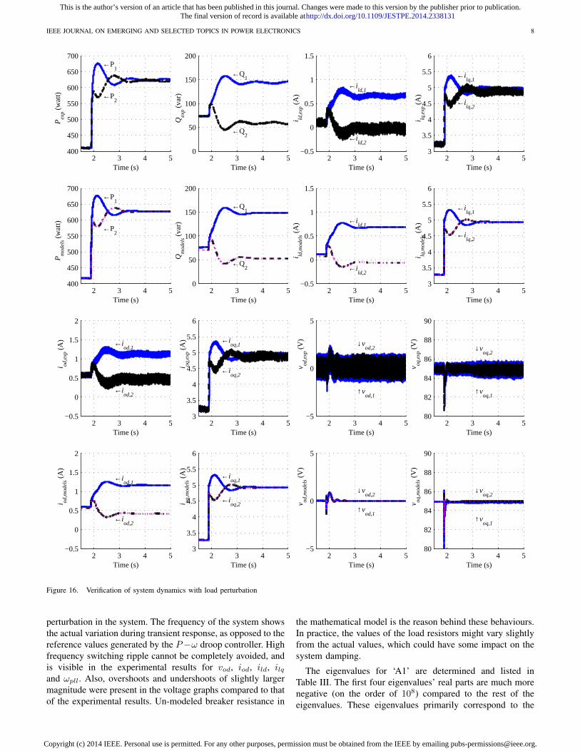
A comparison of the small-signal model prediction simu-lation results and experimental results are shown below Sub-scripts rsquoexprsquo and lsquomodelsrsquo on y-axis labels denote whether thevalues were obtained from the experimental data or from themodel data The load perturbation takes place at t = 1885 sWhen plotted on the same graph results from the averagedmodel simulation and from the mathematical model overlapshown in Fig 15 and Fig 16 This indicates that the resultsfrom the models are consistent The controller was designedsuch that vod is maintained at zero This is shown in thed axis voltage plot From (1) and (2) it is clear that thedynamics of active and reactive power P and Q are dependenton the dynamics of ioq and iod respectively provided thatvoq remains constant This is shown graphically in Fig 16as well In all of the graphs the transient response decaysin 1 s which is acceptable for a power system applicationFor all signals considered the prediction of the mathematicalmodel very closely resembles that found in the simulationand the hardware experiment both in terms of transient andsteady state response In contrast to [19] the proposed small-signal model reaches a proper steady state value after a load
15 2 25 3 35 4 45 5375
376
377
378
Time (s)
ωpl
lexp
(ra
ds)
darrωpll12
15 2 25 3 35 4 45 5375
376
377
378
Time (s)
ωpl
lmod
els (
rad
s)
darrωpll12
Figure 15 Frequency of the system
This is the authorrsquos version of an article that has been published in this journal Changes were made to this version by the publisher prior to publicationThe final version of record is available athttpdxdoiorg101109JESTPE20142338131
Copyright (c) 2014 IEEE Personal use is permitted For any other purposes permission must be obtained from the IEEE by emailing pubs-permissionsieeeorg
IEEE JOURNAL ON EMERGING AND SELECTED TOPICS IN POWER ELECTRONICS 8
2 3 4 5400
450
500
550
600
650
700larrP
1
larrP2
Time (s)
Pex
p (w
att)
2 3 4 5400
450
500
550
600
650
700larrP
1
larrP2
Time (s)
Pm
odel
s (w
att)
2 3 4 50
50
100
150
200
Time (s)Q
exp (
var)
larrQ1
larrQ2
2 3 4 50
50
100
150
200
Time (s)
Qm
odel
s (va
r)
larrQ1
larrQ2
2 3 4 5minus05
0
05
1
15
Time (s)
i lde
xp (
A)
larrild1
larrild2
2 3 4 5minus05
0
05
1
15
Time (s)i ld
mod
els (
A) larri
ld1
larrild2
2 3 4 53
35
4
45
5
55
6
Time (s)
i lqe
xp (
A)
larrilq1
larrilq2
2 3 4 53
35
4
45
5
55
6
Time (s)
i lqm
odel
s (A
)
larrilq1
larrilq2
2 3 4 5minus05
0
05
1
15
2
Time (s)
i ode
xp (
A) larri
od1
larriod2
2 3 4 5minus05
0
05
1
15
2
Time (s)
i odm
odel
s (A
)
larriod1
larriod2
2 3 4 53
35
4
45
5
55
6
Time (s)
i oqe
xp (
A) larri
oq1
larrioq2
2 3 4 53
35
4
45
5
55
6
Time (s)
i oqm
odel
s (A
)
larrioq1
larrioq2
2 3 4 5minus5
0
5
Time (s)
v ode
xp (
V) darrv
od2
uarrvod1
2 3 4 5minus5
0
5
Time (s)
v odm
odel
s (V
)
darrvod2
uarrvod1
2 3 4 580
82
84
86
88
90
Time (s)
v oqe
xp (
V)
darrvoq2
uarrvoq1
2 3 4 580
82
84
86
88
90
Time (s)
v oqm
odel
s (V
)
darrvoq2
uarrvoq1
Figure 16 Verification of system dynamics with load perturbation
perturbation in the system The frequency of the system showsthe actual variation during transient response as opposed to thereference values generated by the Pminusω droop controller Highfrequency switching ripple cannot be completely avoided andis visible in the experimental results for vod iod ild ilqand ωpll Also overshoots and undershoots of slightly largermagnitude were present in the voltage graphs compared to thatof the experimental results Un-modeled breaker resistance in
the mathematical model is the reason behind these behavioursIn practice the values of the load resistors might vary slightlyfrom the actual values which could have some impact on thesystem damping
The eigenvalues for lsquoA1rsquo are determined and listed inTable III The first four eigenvaluesrsquo real parts are much morenegative (on the order of 108) compared to the rest of theeigenvalues These eigenvalues primarily correspond to the
This is the authorrsquos version of an article that has been published in this journal Changes were made to this version by the publisher prior to publicationThe final version of record is available athttpdxdoiorg101109JESTPE20142338131
Copyright (c) 2014 IEEE Personal use is permitted For any other purposes permission must be obtained from the IEEE by emailing pubs-permissionsieeeorg
IEEE JOURNAL ON EMERGING AND SELECTED TOPICS IN POWER ELECTRONICS 9
virtual resistor rn They are not considered when eigenvaluesare plotted in Fig 17 The negative real part of the eigenvaluesobtained from lsquoA1rsquo and lsquoA2rsquo signifies the linearized systemrsquoslocal stability According to Lyapunovrsquos second method forstability analysis the system is asymptotically stable in thesmall-signal sense Although the sub-systems are exponen-tially stable the stability of the overall system cannot beguaranteed [30] [31] This is because the switched systemsmay have divergent trajectories for certain switch signalsHowever these models may be used for a future study ofthe switched system
minus8000 minus6000 minus4000 minus2000 0minus15
minus1
minus05
0
05
1
15x 10
4
Real
Imag
inar
y
Eigenvalues of A1
Figure 17 Partial eigenvalue plot of A1
An eigenvalue analysis investigates the dynamic behaviorof a power system under different characteristic frequenciesor ldquomodesrdquo In a power system it is required that all modesare properly damped to nullify the effect of oscillation due toperturbation in states A well damped system provides goodstability Eigenvalues presented in Table III show that there are15 distinct oscillatory modes in the system A participationfactor analysis was done to identify the states which aremajor participants in those modes Participation factors can bepositive zero or negative A positive participation factor as-sociated with a particular state means that state is contributingto the oscillation of the system A negative participation factorindicates a state that is dampening the system oscillation
The participation factor analysis shows that mode 1 andmode 2 are properly damped in the system However modes3 4 5 and 6 are lightly damped The states in these modes aremore likely to make the system unstable during disturbancesModes 10 11 12 and 13 are low frequency oscillatory andare largely influenced by the states related to the voltage andcurrent controllers Among them mode 12 is not well dampedThis mode can be designated as the lsquoproblem modersquo for thissystem Mode 14 is heavily participated in by the phase angle
of the second inverter This is another low frequency oscilla-tory mode This mode is also influenced by the dynamics ofthe PLL which help dampen the oscillation generated by thephase angle The states relating to the inverter output powersparticipate in mode 15 The natural frequency of oscillation ofthis mode is 8 Hz or 5026 rads This also happens to be thecut-off frequency of the low pass filter used during controllerdesign
From this analysis modes 3 4 5 and 6 are at higheroscillatory frequencies and they have lower damping ratiosThe dq axis output voltages participate heavily in those modesEquations (19) and (20) show that the vodq dynamics aregoverned by the damping resistor Rd along with some otherstate variables As a result any change in Rd will result achange in the output voltage dynamics as well The initialvalue of the damping resistor was chosen based on its ability tosuppress the resonant frequency of the filter A higher dampingresistor may be selected but will contribute additional lossto the system The advantage of using a higher dampingresistance is explained using Table IV which shows the systemeigenvalues when a damping resistor of Rd = 10 Ω isused Another method to increase damping in the system isto include active damping techniques in controller designThis method does not contribute loss to the system Suchcontrollers are beyond the scope of this paper but discussedmore elaborately in [32]
Table IV shows that the higher damping resistance Rd
increases the damping ratio of modes 3 4 5 and 6 Thisimproves the stability margin for the system The low fre-quency oscillatory modes are now the dominant dynamics ofthe system A good controller design for this system wouldachieve higher damping ratios for these modes such that theydecay as quickly as possible after a disturbance This analysisis important to identify the states related to the low frequencyoscillatory modes with lower damping ratios During modelreduction procedures these modes must be retained
A sparsity pattern of lsquoA1rsquo is depicted in Fig 18 The patternshows that there are six regions in the matrix where the non-zero elements are distributed Regions 1 and 3 are formedby DER1 and regions and 2 4 and 5 are formed by DER2Regions 3 and 4 are generated by the inclusion of the virtualresistor rn in the respective inverter buses These regions alsoinclude rnrsquos interaction with the damping resistors and thecoupling inductors Region 5 is formed based on (26) wherethe first inverterrsquos phase angle was set as the reference anglefor the second inverter Region 6 is formed by the loads and thedistribution line If another inverter is added to this system thenthe new sparsity matrix will have additional patterns identicalto those in regions 2 4 and 5 These regions will be locatedon the diagonal of the matrix following the second inverterrsquossparsity pattern
VII CONCLUSION
This work presents an accurate small-signal model of amultiple inverter microgrid system operating in islanded modeThe model is based on the nonlinear equations that describesystem dynamics These nonlinear equations is then linearized
This is the authorrsquos version of an article that has been published in this journal Changes were made to this version by the publisher prior to publicationThe final version of record is available athttpdxdoiorg101109JESTPE20142338131
Copyright (c) 2014 IEEE Personal use is permitted For any other purposes permission must be obtained from the IEEE by emailing pubs-permissionsieeeorg
IEEE JOURNAL ON EMERGING AND SELECTED TOPICS IN POWER ELECTRONICS 10
Table IIIEIGENVALUES OF A1
Index Real (1s) Im (rads) Damping ratio ξ () Natural freq ωo (Hz) Mode Major participants
around stable operating points to develop the small-signalmodel Load perturbation is done to study the system dynam-ics The accuracy of the model is assessed through comparisonto simulation and experimental results An eigenvalue analysisis done using the small-signal model to determine the stabilityof the system Low and high frequency oscillatory modes areidentified from the eigenvalue analysis A participation factoranalysis is included to identify the states contributing to thedifferent oscillatory modes It is found that some of theseoscillatory modes can be controlled using proper dampingresistors A sparsity pattern of the system is investigated
The most important contribution of this paper is the proposedmodel of an islanded microgrid and its ability to accuratelypredict the dynamic response of the system It is possible thatsimilar power system networks could be accurately developedas switched autonomous systems Future work for this project
This is the authorrsquos version of an article that has been published in this journal Changes were made to this version by the publisher prior to publicationThe final version of record is available athttpdxdoiorg101109JESTPE20142338131
Copyright (c) 2014 IEEE Personal use is permitted For any other purposes permission must be obtained from the IEEE by emailing pubs-permissionsieeeorg
IEEE JOURNAL ON EMERGING AND SELECTED TOPICS IN POWER ELECTRONICS 11
will include determination and application of a proper modelreduction technique to reduce the fast decaying states Alsosystem modeling with capacitive and nonlinar load are con-sidered as separate research objectives
REFERENCES
[1] M Smith and D Ton ldquoKey connections The US Department ofEnergyrsquos microgrid initiativerdquo IEEE Power Energy Mag vol 11 no 4pp 22ndash27 Jul 2013
[2] D Boroyevich I Cvetkovic R Burgos and D Dong ldquoIntergrid Afuture electronic energy networkrdquo IEEE J Emerg Sel Top PowerElectron vol 1 no 3 pp 127ndash138 Sep 2013
[3] R H Lasseter ldquoSmart distribution Coupled microgridsrdquo Proc IEEEvol 99 no 6 pp 1074ndash1082 Jun 2011
[4] mdashmdash ldquoMicrogridsrdquo in Power Engineering Society Winter Meeting 2002IEEE vol 1 2002 p 305ndash308
[5] I Grau L M Cipcigan N Jenkins and P Papadopoulos ldquoMicrogridintentional islanding for network emergenciesrdquo in Universities PowerEngineering Conference (UPEC) 2009 Proceedings of the 44th Inter-national 2009 p 1ndash5
[6] J Peas Lopes C Moreira and A Madureira ldquoDefining control strate-gies for MicroGrids islanded operationrdquo IEEE Trans Power Systvol 21 no 2 pp 916ndash924 2006
[7] T Green and M Prodanovic ldquoControl of inverter-based micro-gridsrdquoElectric Power Systems Research vol 77 no 9 pp 1204ndash1213 Jul2007
[8] H-K Kang S-J Ahn and S-I Moon ldquoA new method to determinethe droop of inverter-based DGsrdquo in Power amp Energy Society GeneralMeeting 2009 PESrsquo09 IEEE 2009 p 1ndash6
[9] S Tabatabaee H R Karshenas A Bakhshai and P Jain ldquoInvestigationof droop characteristics and XR ratio on small-signal stability ofautonomous microgridrdquo in Power Electronics Drive Systems and TechConf (PEDSTC) 2011 2nd 2011 pp 223ndash228
[10] W Yao M Chen J Matas J M Guerrero and Z-M Qian ldquoDesign andanalysis of the droop control method for parallel inverters consideringthe impact of the complex impedance on the power sharingrdquo IEEETrans Ind Electron vol 58 no 2 pp 576ndash588 Feb 2011
[11] C-T Lee C-C Chu and P-T Cheng ldquoA new droop control methodfor the autonomous operation of distributed energy resource interfaceconvertersrdquo IEEE Trans Power Electron vol 28 no 4 pp 1980ndash1993Apr 2013
[12] Y Guan Y Wang Z Yang R Cao and H Xu ldquoControl strategyfor autonomous operation of three-phase inverters dominated microgridunder different line impedancerdquo in Int Conf on Electrical Machinesand Systems (ICEMS) 2011 pp 1ndash5
[13] T L Vandoorn B Meersman L Degroote B Renders and L Vande-velde ldquoA control strategy for islanded microgrids with DC-Link voltagecontrolrdquo IEEE Trans Power Deliv vol 26 no 2 pp 703ndash713 Apr2011
[14] T L Vandoorn B Renders B Meersman L Degroote and L Van-develde ldquoReactive power sharing in an islanded microgridrdquo in IntUniversities Power Engineering Conf (UPEC) 2010 pp 1ndash6
[15] T L Vandoorn B Renders L Degroote B Meersman and L Van-develde ldquoActive load control in islanded microgrids based on the gridvoltagerdquo IEEE Trans Smart Grid vol 2 no 1 pp 139ndash151 Mar 2011
[16] F Katiraei M Iravani and P Lehn ldquoSmall-signal dynamic modelof a micro-grid including conventional and electronically interfaceddistributed resourcesrdquo IET Generation Transmission amp Distributionvol 1 no 3 pp 369ndash378 2007
[17] Y Zhang Z Jiang and X Yu ldquoSmall-signal modeling and analysisof parallel-connected voltage source invertersrdquo in IEEE Int PowerElectronics and Motion Control Conf 2009 pp 377ndash383
[18] E A A Coelho P C Cortizo and P F D Garcia ldquoSmall-signal stabil-ity for parallel-connected inverters in stand-alone AC supply systemsrdquoIEEE Trans Ind App vol 38 no 2 pp 533ndash542 2002
[19] N Pogaku M Prodanovic and T C Green ldquoModeling analysis andtesting of autonomous operation of an inverter-based microgridrdquo IEEETrans Power Electron vol 22 no 2 pp 613ndash625 Mar 2007
[20] Y Mohamed and E El-Saadany ldquoAdaptive decentralized droop con-troller to preserve power sharing stability of paralleled inverters indistributed generation microgridsrdquo IEEE Trans Power Electron vol 23no 6 pp 2806ndash2816 Nov 2008
[21] M A Hassan and M A Abido ldquoOptimal design of microgrids in au-tonomous and grid-connected modes using particle swarm optimizationrdquoIEEE Trans Power Electron vol 26 no 3 pp 755ndash769 Mar 2011
[22] R M dos Santos Filho P F Seixas and P C Cortizo ldquoA comparativestudy of three-phase and single-phase PLL algorithms for grid-connected systemsrdquo in Proc INDUSCON Conf Rec 2006 [Online]Available httpwwwcpdeeufmgbrdocumentosPublicacoesDefesas853EPA-VII_5pdf
[23] V Kaura and V Blasko ldquoOperation of a phase locked loopsystem under distorted utility conditionsrdquo Industry Applications IEEETransactions on vol 33 no 1 p 58ndash63 1997 [Online] Availablehttpieeexploreieeeorgxplsabs_alljsparnumber=567077
[24] J Oumlgren ldquoPLL design for inverter grid connection Simulations for idealand non-ideal grid conditionsrdquo Masterrsquos thesis Uppsala University2010 [Online] Available httpwwwdiva-portalorgsmashrecordjsfpid=diva2430787
[25] P Krause ldquoThe method of symmetrical components derived by referenceframe theoryrdquo IEEE Trans Power Appar Syst vol PAS-104 no 6 pp1492ndash1499 1985
[26] M Rasheduzzaman J Mueller and J W Kimball ldquoSmall-signal mod-eling of a three-phase isolated inverter with both voltage and frequencydroop controlrdquo in Proceedings of the IEEE Applied Power ElectronicsConference 2014 2014 pp 1008ndash1015
[27] J Dannehl M Liserre and F W Fuchs ldquoFilter-based active damping ofvoltage source converters with LCL filterrdquo IEEE Trans Ind Electronvol 58 no 8 pp 3623ndash3633 Aug 2011
[28] M Liserre F Blaabjerg and S Hansen ldquoDesign and control of an LCL-Filter-Based three-phase active rectifierrdquo IEEE Trans Ind App vol 41no 5 pp 1281ndash1291 Sep 2005
[29] H Cha and T-K Vu ldquoComparative analysis of low-pass output filterfor single-phase grid-connected photovoltaic inverterrdquo in Applied PowerElectronics Conference and Exposition (APEC) 2010 Twenty-FifthAnnual IEEE IEEE 2010 p 1659ndash1665 [Online] Availablehttpieeexploreieeeorgxplsabs_alljsparnumber=5433454
[30] D Liberzon Switching in Systems and Control Boston MABirkhauser Boston Imprint Birkhauser 2003
[31] M Rasheduzzaman T Paul and J W Kimball ldquoMarkov jump linearsystem analysis of microgridrdquo in Proc of American Control Conf (ACC)2014
[32] C Bao X Ruan X Wang W Li D Pan and K Weng ldquoStep-by-stepcontroller design for LCL-Type grid-connected inverter with capacitor-current-feedback active-dampingrdquo IEEE Trans Power Electron vol 29no 3 pp 1239ndash1253 Mar 2014
This is the authorrsquos version of an article that has been published in this journal Changes were made to this version by the publisher prior to publicationThe final version of record is available athttpdxdoiorg101109JESTPE20142338131
Copyright (c) 2014 IEEE Personal use is permitted For any other purposes permission must be obtained from the IEEE by emailing pubs-permissionsieeeorg
IEEE JOURNAL ON EMERGING AND SELECTED TOPICS IN POWER ELECTRONICS 2
play an important role in ensuring stability of the systemwere ignored Additionally the model was designed such thata load current transient was used as a perturbation inputwhile in practice a change in impedance was observed duringthe transient analysis This improper perturbation techniqueresulted in a significant reactive power mismatch betweenthe experimental results and the results obtained from themodel Another small-signal model was derived in [20] Againthe model did not include the passive damping properties ofthe filter Results from this model were not validated againstthose from a hardware experiment The models from thelast two papers did not include the dynamics of the PLL toverify system frequency during load perturbation A small-signal model was developed in [21] which included the PLLdynamics and a damping resistor in the filter Once againthe model was not validated against the experimental resultsAlso the input matrix was defined in such a way that it didnot reflect the load perturbation in the system
As a solution to the issues associated with these priormodels a more accurate small-signal model is presented inthis paper The development and verification of this model is asfollows First the proposed control structure is described usinga block diagram A set of nonlinear equations is then derivedfrom the controller blocks and the plant These equationsare linearized around stable operating points To simulate theeffect of the load perturbation a switched system arrangementis implemented Finally the transient response predicted by themathematical model is verified against both the simulation andexperimental results The proposed model is intended to serveas a building block for control of more complex systems ofmodern distributed generation sources
II OVERVIEW OF THE SYSTEM
The islanded microgrid under consideration is presented inFig 1 Each inverter is connected to a respective bus througha filter Variable passive loads connected to these buses areconsidered as local loads Depending on the status of thesystem either grid-connected or islanded the switch at thepoint of common coupling (PCC) may connect the system tothe main grid A distribution line with impedance ZL is usedto couple the inverter buses While the proposed system canoperate in either grid-connected mode or as an autonomoussystem only the autonomous operation will be considered inthis paper
ZL
Main
grid
DER1 DER2
Bus1 Bus2
PCC
Line
Load1 Load2
Microgrid
1 2
Figure 1 Proposed microgrid architecture
In autonomous operation the inverter is controlled using thedroop control method An individual inverter control strategyis depicted in Fig 2 The output of the inverter is passedthrough an LCL filter to reject the high frequency switchingnoise The filtered voltage and current measurements are thenconverted to dq axis components using a reference frame trans-formation The inverterrsquos output power is calculated based onthese measurements The calculated power is passed througha low pass filter and sent to the droop controllers Droopcontrollers set voltage and frequency references based on thecurrent level of active and reactive power being generatedThese voltage and frequency references are then comparedwith the measured voltage and frequency The lsquoerror signalrsquoobtained by comparing the reference values and measuredvalues are passed through PI controllers to generate referencesfor the current flowing through the output filter inductorThese reference current signals are then compared with thecorresponding measured filter inductor currents and are passedthrough another set of PI controllers to produce voltagecommands These voltage values appear across the input ofthe LCL filter The coupling inductor of the filter is used toconnect the inverter to the bus A resistor in series with thefilter capacitor ensures the proper damping of the resonantfrequency associated with the output filter
As mentioned before a frequency measurement is neededfor voltage controllers to operate The frequency of the systemis measured by forcing the d axis component of the voltageto zero in a dq based PLL This PLL not only measures thefrequency of the system but also calculates the phase angle ofthe voltage This angle is used to make all the conversionsbetween stationary and synchronous reference frames Allcontrollers and filters are modeled in the individual referenceframe local to each inverter as determined by the phase anglefrom the PLL The invertersrsquo dynamics are influenced by theoutput filter coupling inductor average power calculationPLL droop controllers and current controllers The overallsystem dynamics include those of each individual inverterload and the distribution line between them
III SYSTEM MODELING IN STATE-SPACE FORM
A Nonlinear Equations of the Inverter ModelIn this section the controllers shown as blocks in Fig 2 are
analyzed and expressed in terms of mathematical equationsThese equations are nonlinear and need to be linearized aroundan operating point to study the system dynamics
1) Average Power Calculation The dq axis output voltageand current measurements are used to calculate the instanta-neous active power (p) and reactive power (q) generated bythe inverter
p =3
2(vodiod + voqioq) (1)
q =3
2(voqiod minus vodioq) (2)
Instantaneous powers are then passed through low pass filterswith the corner frequency ωc to obtain the filtered outputpower
This is the authorrsquos version of an article that has been published in this journal Changes were made to this version by the publisher prior to publicationThe final version of record is available athttpdxdoiorg101109JESTPE20142338131
Copyright (c) 2014 IEEE Personal use is permitted For any other purposes permission must be obtained from the IEEE by emailing pubs-permissionsieeeorg
IEEE JOURNAL ON EMERGING AND SELECTED TOPICS IN POWER ELECTRONICS 3
2) Droop Equations In grid-connected mode the inverterrsquosoutput voltage is set by the grid voltage magnitude ThePLL ensures proper tracking of grid phase so that inverteroutput remains synchronized to the grid During islandedoperation the inverter does not have these externally generatedreference signals As a result the inverter must generate itsown frequency and voltage magnitude references using thedroop equations The references are generated using conven-tional P minus ω and Q minus V droop equations Fig 3 shows thecharacteristics of these droop curves
ω1
P1
ω2
ω
P
V1
Q1
V2
V
QP2 Q2
1 2
2 1
mP P
1 2
2 1
V Vn
Q Q
Figure 3 Droop characteristic curves
ωlowast = ωn minusmP (5)
voqlowast = Voqn minus nQ (6)
3) Phase Locked Loop (PLL) A PLL is required to mea-sure the actual frequency of the system A dq based PLL waschosen [22] [23] [24] [23] The PLL input is the d axiscomponent of the voltage measured across the filter capacitorTherefore the phase is locked such that vod = 0 (Fig 4) Someresearchers instead set the PLL to lock such that voq = 0which would essentially swap d-axis and q-axis quantitiesthroughout the remainder of this work There are three statesassociated with this PLL architecture
377
odv0
kpPLL
kiPLL1s 1s
c PLL
c PLLs
od fv
Figure 4 PLL used for the DER
vodf = ωcPLLvod minus ωcPLLvodf (7)
ϕPLL = minusvodf (8)
δ = ωPLL (9)
ωPLL = 377minus kpPLLvodf + kiPLLϕPLL (10)
4) Voltage Controllers The reference frequency and volt-age magnitude generated by the droop equations are usedas set point values for the voltage controllers Standard PIcontrollers are used for this purpose shown in Fig 5 Theprocess variables are the angular frequency ω from the PLLand the measured q axis voltage (voq)
This is the authorrsquos version of an article that has been published in this journal Changes were made to this version by the publisher prior to publicationThe final version of record is available athttpdxdoiorg101109JESTPE20142338131
Copyright (c) 2014 IEEE Personal use is permitted For any other purposes permission must be obtained from the IEEE by emailing pubs-permissionsieeeorg
IEEE JOURNAL ON EMERGING AND SELECTED TOPICS IN POWER ELECTRONICS 4
5) Current Controllers Another set of PI controllers areused for the current controllers as shown in Fig 6 Thesecontrollers take the difference between the commanded filterinductor currents (ildqlowast) the measured filter inductor currents(ildq) and produce commanded voltage values (vidqlowast) Thevalues of correspond to the inverter output voltages before theLCL filter Cross coupling component terms are eliminated inthese controllers as well
vid
ilq
viq
ild
ilq
ilq
ild
ild 1s1s
kpcd
kicd
-ωnLf
kpcq
kicq
ωnLf
Figure 6 Current controllers
γd = ildlowastminusild vid
lowast = minusωnLf ilq +kicdγd+kpcdγd (13)
γq = ilqlowast minus ilq viq
lowast = ωnLf ild + kicqγq + kpcqγq (14)
B LCL Filter
The filter used for a DER is shown in Fig 7 Withoutany major inaccuracies we can assume that the commandedvoltage (vlowastidq) appears at the input of the filter inductorie vlowastidq = vidq This approach neglects only the lossesin the IGBT and diodes The resistors rc and rf are theparasitic resistances of the inductors A damping resistor Rd
is connected in series with the filter capacitor The capacitorrsquosESR is not considered as it can be lumped into Rd The stateequations governing the filter dynamics are presented below
vidq
iℓdq
Lf
Cf
Rd
rf vodq
iodq
vbdqLc rc
Figure 7 LCL filter for the DER
ild =1
Lf(minusrf ild + vid minus vod) + ωPLLilq (15)
ilq =1
Lf(minusrf ilq + viq minus voq)minus ωPLLild (16)
iod =1
Lc(minusrciod + vod minus vbd) + ωPLLioq (17)
ioq =1
Lc(minusrcioq + voq minus vbq)minus ωPLLiod (18)
vod =1
Cf(ild minus iod) + ωPLLvoq +Rd(ild minus iod) (19)
voq =1
Cf(ilq minus ioq)minus ωPLLvod +Rd(ilq minus ioq) (20)
C Equations for the Load
The loads for this system are chosen as combination of resis-tors and inductors (RL loads) A typical RL load connected toan inverter bus is shown in Fig 8 Line lsquoarsquo connected to the busrepresents the base load and line lsquobrsquo works as a variable loadfor that bus In order to check the systemrsquos dynamic behaviora load perturbation is done on lsquobrsquo Line lsquobrsquo appears in parallelto lsquoarsquo when the breaker closes the contact State equationsdescribing the load dynamics are given below
Similar to loads the distribution line parameters consist ofresistance and inductance Resistor rline represents the copperloss component of the line Inductor Lline is considered as thelumped inductance resulting from long line cables Assumingthat the line is connected between i-th and j-th bus of thesystem the line dynamics are represented as follows
vbDQi vbDQjrlineLline
ilineDQij
Figure 9 Line configuration
ilineDij =1
Lline(minusrlineilineD + vbDi minus vbDj)+ωPLLilineQ
(23)
ilineQij =1
Lline(minusrlineilineQ + vbQi minus vbQj)minusωPLLilineD
(24)The frequency is constant throughout the system so theequations for the load and line dynamics can use the termderived from the ωPLL of the first inverter The variablesubscript with upper case DQ denotes measurements fromthe global reference frame Since the system does not have afixed grid connected to it the first inverterrsquos phase angle canbe arbitrarily set as the reference for the entire system Thisresults in a change in the reference angle calculation whensmall-signal modelrsquos matrices are derived The new phaseangle derivations for DER1 and DER2 are given in (25) and
This is the authorrsquos version of an article that has been published in this journal Changes were made to this version by the publisher prior to publicationThe final version of record is available athttpdxdoiorg101109JESTPE20142338131
Copyright (c) 2014 IEEE Personal use is permitted For any other purposes permission must be obtained from the IEEE by emailing pubs-permissionsieeeorg
IEEE JOURNAL ON EMERGING AND SELECTED TOPICS IN POWER ELECTRONICS 5
(26) where ωPLL1 and ωPLL2 come from DER1 and DER2respectively
δ1 = ωPLL1 minus ωPLL1 = 0 (25)
δ2 = ωPLL1 minus ωPLL2 (26)
E Linearized Model of the System
Each inverter system contains 15 states and each load andline model contain 2 states A total of 36 states are containedin the full two inverter islanded microgrid system The statesare
xinv1 =[δ1 P1 Q1 ϕd1 ϕq1 γd1 γq1 ild1 ilq1
vod1 voq1 iod1 ioq1 ϕPLL1 vod1f ](27)
xinv2 =[δ2 P2 Q2 ϕd2 ϕq2 γd2 γq2 ild2 ilq2
vod2 voq2 iod2 ioq2 ϕPLL2 vod2f ](28)
xload = [iloadD1 iloadQ1 iloadD2 iloadQ2] (29)
xline = [ilineD21 ilineQ21] (30)
The states of the system under consideration are then
x = [xinv1 xinv2 xload xline]T (31)
These nonlinear equations are linearized around stable oper-ating points and a state-space equation of the form (32) isgenerated using Matlabrsquos symbolic math toolbox
˙x = Ax+Bu (32)
Where the inputs are defined as
u = [vbD1 vbQ1 vbD2 vbQ2]T (33)
F Virtual Resistor Method
When bus voltages were used as an input to the system as inprevious microgrid models effects of load perturbation couldnot be accurately predicted In practice the only perturbationthat occurs in the system comes from the step change inload A method is needed to include the terms relating tothe bus voltages in the system lsquoArsquo matrix This effectivelytranslates the inputs defined in (33) to states To do this avirtual resistor with high resistance can be assumed connectedat the inverter bus This resistor (rn) has a negligible impacton system dynamics Using KVL the equations describingthe bus voltage in terms of the inverter load currents and linecurrents can be expressed This is shown in (34) and (35)
vbDi = rn (ioDi + ilineDi minus iloadDi) (34)
vbQi = rn (ioQi + ilindQi minus iloadQi) (35)
ioDQi
ilineDQi
iloadDQi
vbDQi
rn
Figure 10 Virtual resistor at a DER bus
G Reference Frame Transformation
As previously discussed inverter bus 1 serves as the sys-temrsquos reference and consequently is labeled as the globalreference frame Each inverter operates in its own localreference frame The individual inverter state equations arederived in terms of their individual local reference frame Atransformation is necessary to translate between values definedin the local reference frame to the global reference frameAn application of this transformation is shown graphicallyin Fig 11 Again the difference in subscript capitalizationdenotes whether the quantity is defined in the local or globalreference frame
vbdq
iodq
Inverter Bus
3ɸ Inverter
and
LCL filter
vbDQ
Local to global
reference frame
ioDQ
Global to local
reference frame
To the rest
of the system
Figure 11 Reference frame transformation
[fDfQ
]global
=
[cos θ sin θminus sin θ cos θ
] [fdfq
]local
(36)
[fdfq
]local
=
[cos θ minus sin θsin θ cos θ
] [fDfQ
]global
(37)
Where θ is the difference between the global reference phaseand the local reference phase as depicted in Fig 12
d1 = D
q2
q1 = Q
d2
1 0global
2
Figure 12 Transformation angle
This is the authorrsquos version of an article that has been published in this journal Changes were made to this version by the publisher prior to publicationThe final version of record is available athttpdxdoiorg101109JESTPE20142338131
Copyright (c) 2014 IEEE Personal use is permitted For any other purposes permission must be obtained from the IEEE by emailing pubs-permissionsieeeorg
IEEE JOURNAL ON EMERGING AND SELECTED TOPICS IN POWER ELECTRONICS 6
This transformation [25] is used to refer the virtual resistorequations that are defined in the global reference frame tothe local reference frame The equations (36) (37) and thereference frame transformations can then be linearized andincluded in the symbolic lsquoArsquo matrix A new state matrix lsquoAsysrsquothen describes the system in state space form The states ofthis new system are the same as those given in (31)
˙x = Asysx (38)
IV EVALUATION OF THE MATHEMATICAL MODEL
The autonomous system described by the matrix lsquoAsysrsquoneeds to be linearized around stable operating points Thereare two ways of finding these operating points One methodis to set the nonlinear state equations to zero as (x = 0)Another approach is to simulate the averaged model in PLECSto determine numerical solutions to the nonlinear systemequations Because both methods yielded same results thesimulation based method was used for convenience
As mentioned previously loads are connected to inverterbuses as in Fig 8 Initially load lsquoarsquo at bus 1 and bus 2 isswitched on A set of operating points is determined for thisloading condition These operating points are given in (39)A new set of operating points is determined after applyinglsquobrsquo parallel to the initial load at bus 1 to simulate a loadperturbation Rload1 Lload1 and Rload2 Lload2 are the initialloads at bus 1 and bus 2 respectively Rpert1 and Lpert1 arethe new loads added to bus 1 New operating points for theequivalent load impedance seen at bus 1 are obtained Theseoperating points are given in (40) The dynamic responsewhen changing between these two operating points yieldsthe mathematical modelrsquos prediction for a load step changetransient [26] The controller gains and system parameters arelisted in Table I and Table II
Fig 13 shows the small-signal model evaluation arrange-ment in Simulink Matrices lsquoA1rsquo and lsquoA2rsquo are obtained throughlinearization around stable operating points given in (39) and(40) Operating points are arranged in the order given in (31)
ioq
gt= 051
s
A2 u
A1 u
X2
X1
d
P
Q
Figure 13 Small-signal simulation arrangement in Simulink
Table ICONTROLLER GAINS
PI gains for Parameter Value
Voltage kpvd kpvq 050
controllers kivd kivq 250
Current kpcd kpcq 100
controllers kicd kicq 100
PLL kpPLL 025
controller kiPLL 200
Table IISYSTEM PARAMETERS AND INITIAL CONDITIONS
Parameter Value Parameter Value
Lf 420 mH rf 050 Ω
Lc 050 mH rc 009 Ω
Cf 15 microf Rd 2025 Ω
ωc 5026 rads ωn 377 rads
ωcPLL 785398 rads ωPLL 377 rads
m 11000 radWs n 11000 VV ar
rn 1000 Ω Voqn 850 V
Rload1 25 Ω Lload1 15 mH
Rload2 25Ω Lload2 750 mH
Rpert1 25 Ω Lpert1 750 mH
rline 015 Ω Lline 040 mH
VbD1 060585 V VbQ1 84516 V
VbD2 063937 V VbQ2 84529 V
X1 =[0 41818 76104 00034259 013152 00014666
086569 01198 32871 0041403 84923 059961
32813minus020887 0042771 000038 41595 7012
0001539 013084 0001221 086564 00719 32716
0042439 84929 055145 32659minus020868 0042
074987 32113 040117 33359 015028minus00699]T
(39)
X2 =[0 62715 14807 0027375 019731 00035517
087317 06842 49328minus00037896 84835 11644
4927minus03135 000253minus00036217 62713 53113
minus 0002506 019709minus00001836 087411minus006246
49273 00032628 84959 041577 49216minus031357
minus 000298 116 6518 04117 333 00042 15911]T
(40)
These expressions (39)-(40) represent the steady-state val-ues of the state vector x (from (31)) at two load operatingpoints with and without Rpert1 and Lpert1 evaluated for theparameters given in Tables I and II
V EXPERIMENT SETUP
In order to validate the results of the mathematical modelthe dynamic response is compared against those of a simula-tion and experiment in hardware An averaged model of theproposed system is simulated in PLECS This average modelis perturbed through a load change in bus 1 as discussed inthe previous sections In hardware implementation a Texas
This is the authorrsquos version of an article that has been published in this journal Changes were made to this version by the publisher prior to publicationThe final version of record is available athttpdxdoiorg101109JESTPE20142338131
Copyright (c) 2014 IEEE Personal use is permitted For any other purposes permission must be obtained from the IEEE by emailing pubs-permissionsieeeorg
IEEE JOURNAL ON EMERGING AND SELECTED TOPICS IN POWER ELECTRONICS 7
(a) Inverter with sensors (b) LCL filter
(c) Load setup
Figure 14 Partial photograph of the test bed a DER2 b LCL filter c Loadsat bus 1
Instruments TMS320F28335 digital signal processor was usedto apply the control system to a 10 kW inverter designedaround an Infineon BSM30GP60 IGBT module A dc sourcewas connected directly to the dc link and the three phaseoutputs were connected to the loads Space vector modulation(SVPWM) was used as the switching scheme at a frequencyof 10 kHz The experimental results collected correspond tothe actual values in the DSP which were logged in real timeThis was accomplished through transmission of the requiredvalues over serial connections to a host computer as theinternal storage capacity of the DSP was not sufficient tosave the large volumes of data generated by the logs In thesame way as in the simulation the system was perturbed bymanually switching between load configurations and loggingthe dynamic response A diagram of the experimental setupwas provided in Fig 1 Because we are considering theislanded case the switch shown as the PCC to the main gridin Fig 1 was open for the entire experiment Fig 14 showsa partial photograph of the experimental setup includingsensors and circuit board output filter and load configurationAlthough the derivation above only considered one DER bothof the DERs connected to the islanded microgrid had similarconfiguration Each inverter had an individual DSP used forthe controller implementation
LCL filters with damping resistors are used at the IGBToutput terminals The impact of using an LCL filter in this kindof system is discussed in [27] The filter was designed suchthat the resonant frequency was greater than 10 times the linefrequency and less than half the switching frequency [28] Theresonant frequency of this wye-connected LCL filter ignoringparasitic resistances was found to be 194 kHz using (41)The ratio of Lf to Lc was adequate for improving the totalharmonic distortion (THD) and providing better bus voltageregulation
fres sim=1
2π
radicLf + Lc
LfLcCf
sim= 1944 kHz (41)
Passive damping using a damping resistor (Rd) in serieswith the filter capacitor was used to suppress the resonancefrequency of the LCL filter The value of Rd was foundusing [29]
Rd =1
3ωresCf= 18193 Ω (42)
A resistor of this value was unavailable during the time thetest bed was built As a result Rd with slightly higher valuewas used as listed in the Table II Although the results wereobtained with a grid voltage of 60 VLN the small-signalmodels are equally applicable to 120 VLN voltage levelscommonly used at the distribution side of a power system
VI RESULTS AND DISCUSSIONS
A comparison of the small-signal model prediction simu-lation results and experimental results are shown below Sub-scripts rsquoexprsquo and lsquomodelsrsquo on y-axis labels denote whether thevalues were obtained from the experimental data or from themodel data The load perturbation takes place at t = 1885 sWhen plotted on the same graph results from the averagedmodel simulation and from the mathematical model overlapshown in Fig 15 and Fig 16 This indicates that the resultsfrom the models are consistent The controller was designedsuch that vod is maintained at zero This is shown in thed axis voltage plot From (1) and (2) it is clear that thedynamics of active and reactive power P and Q are dependenton the dynamics of ioq and iod respectively provided thatvoq remains constant This is shown graphically in Fig 16as well In all of the graphs the transient response decaysin 1 s which is acceptable for a power system applicationFor all signals considered the prediction of the mathematicalmodel very closely resembles that found in the simulationand the hardware experiment both in terms of transient andsteady state response In contrast to [19] the proposed small-signal model reaches a proper steady state value after a load
15 2 25 3 35 4 45 5375
376
377
378
Time (s)
ωpl
lexp
(ra
ds)
darrωpll12
15 2 25 3 35 4 45 5375
376
377
378
Time (s)
ωpl
lmod
els (
rad
s)
darrωpll12
Figure 15 Frequency of the system
This is the authorrsquos version of an article that has been published in this journal Changes were made to this version by the publisher prior to publicationThe final version of record is available athttpdxdoiorg101109JESTPE20142338131
Copyright (c) 2014 IEEE Personal use is permitted For any other purposes permission must be obtained from the IEEE by emailing pubs-permissionsieeeorg
IEEE JOURNAL ON EMERGING AND SELECTED TOPICS IN POWER ELECTRONICS 8
2 3 4 5400
450
500
550
600
650
700larrP
1
larrP2
Time (s)
Pex
p (w
att)
2 3 4 5400
450
500
550
600
650
700larrP
1
larrP2
Time (s)
Pm
odel
s (w
att)
2 3 4 50
50
100
150
200
Time (s)Q
exp (
var)
larrQ1
larrQ2
2 3 4 50
50
100
150
200
Time (s)
Qm
odel
s (va
r)
larrQ1
larrQ2
2 3 4 5minus05
0
05
1
15
Time (s)
i lde
xp (
A)
larrild1
larrild2
2 3 4 5minus05
0
05
1
15
Time (s)i ld
mod
els (
A) larri
ld1
larrild2
2 3 4 53
35
4
45
5
55
6
Time (s)
i lqe
xp (
A)
larrilq1
larrilq2
2 3 4 53
35
4
45
5
55
6
Time (s)
i lqm
odel
s (A
)
larrilq1
larrilq2
2 3 4 5minus05
0
05
1
15
2
Time (s)
i ode
xp (
A) larri
od1
larriod2
2 3 4 5minus05
0
05
1
15
2
Time (s)
i odm
odel
s (A
)
larriod1
larriod2
2 3 4 53
35
4
45
5
55
6
Time (s)
i oqe
xp (
A) larri
oq1
larrioq2
2 3 4 53
35
4
45
5
55
6
Time (s)
i oqm
odel
s (A
)
larrioq1
larrioq2
2 3 4 5minus5
0
5
Time (s)
v ode
xp (
V) darrv
od2
uarrvod1
2 3 4 5minus5
0
5
Time (s)
v odm
odel
s (V
)
darrvod2
uarrvod1
2 3 4 580
82
84
86
88
90
Time (s)
v oqe
xp (
V)
darrvoq2
uarrvoq1
2 3 4 580
82
84
86
88
90
Time (s)
v oqm
odel
s (V
)
darrvoq2
uarrvoq1
Figure 16 Verification of system dynamics with load perturbation
perturbation in the system The frequency of the system showsthe actual variation during transient response as opposed to thereference values generated by the Pminusω droop controller Highfrequency switching ripple cannot be completely avoided andis visible in the experimental results for vod iod ild ilqand ωpll Also overshoots and undershoots of slightly largermagnitude were present in the voltage graphs compared to thatof the experimental results Un-modeled breaker resistance in
the mathematical model is the reason behind these behavioursIn practice the values of the load resistors might vary slightlyfrom the actual values which could have some impact on thesystem damping
The eigenvalues for lsquoA1rsquo are determined and listed inTable III The first four eigenvaluesrsquo real parts are much morenegative (on the order of 108) compared to the rest of theeigenvalues These eigenvalues primarily correspond to the
This is the authorrsquos version of an article that has been published in this journal Changes were made to this version by the publisher prior to publicationThe final version of record is available athttpdxdoiorg101109JESTPE20142338131
Copyright (c) 2014 IEEE Personal use is permitted For any other purposes permission must be obtained from the IEEE by emailing pubs-permissionsieeeorg
IEEE JOURNAL ON EMERGING AND SELECTED TOPICS IN POWER ELECTRONICS 9
virtual resistor rn They are not considered when eigenvaluesare plotted in Fig 17 The negative real part of the eigenvaluesobtained from lsquoA1rsquo and lsquoA2rsquo signifies the linearized systemrsquoslocal stability According to Lyapunovrsquos second method forstability analysis the system is asymptotically stable in thesmall-signal sense Although the sub-systems are exponen-tially stable the stability of the overall system cannot beguaranteed [30] [31] This is because the switched systemsmay have divergent trajectories for certain switch signalsHowever these models may be used for a future study ofthe switched system
minus8000 minus6000 minus4000 minus2000 0minus15
minus1
minus05
0
05
1
15x 10
4
Real
Imag
inar
y
Eigenvalues of A1
Figure 17 Partial eigenvalue plot of A1
An eigenvalue analysis investigates the dynamic behaviorof a power system under different characteristic frequenciesor ldquomodesrdquo In a power system it is required that all modesare properly damped to nullify the effect of oscillation due toperturbation in states A well damped system provides goodstability Eigenvalues presented in Table III show that there are15 distinct oscillatory modes in the system A participationfactor analysis was done to identify the states which aremajor participants in those modes Participation factors can bepositive zero or negative A positive participation factor as-sociated with a particular state means that state is contributingto the oscillation of the system A negative participation factorindicates a state that is dampening the system oscillation
The participation factor analysis shows that mode 1 andmode 2 are properly damped in the system However modes3 4 5 and 6 are lightly damped The states in these modes aremore likely to make the system unstable during disturbancesModes 10 11 12 and 13 are low frequency oscillatory andare largely influenced by the states related to the voltage andcurrent controllers Among them mode 12 is not well dampedThis mode can be designated as the lsquoproblem modersquo for thissystem Mode 14 is heavily participated in by the phase angle
of the second inverter This is another low frequency oscilla-tory mode This mode is also influenced by the dynamics ofthe PLL which help dampen the oscillation generated by thephase angle The states relating to the inverter output powersparticipate in mode 15 The natural frequency of oscillation ofthis mode is 8 Hz or 5026 rads This also happens to be thecut-off frequency of the low pass filter used during controllerdesign
From this analysis modes 3 4 5 and 6 are at higheroscillatory frequencies and they have lower damping ratiosThe dq axis output voltages participate heavily in those modesEquations (19) and (20) show that the vodq dynamics aregoverned by the damping resistor Rd along with some otherstate variables As a result any change in Rd will result achange in the output voltage dynamics as well The initialvalue of the damping resistor was chosen based on its ability tosuppress the resonant frequency of the filter A higher dampingresistor may be selected but will contribute additional lossto the system The advantage of using a higher dampingresistance is explained using Table IV which shows the systemeigenvalues when a damping resistor of Rd = 10 Ω isused Another method to increase damping in the system isto include active damping techniques in controller designThis method does not contribute loss to the system Suchcontrollers are beyond the scope of this paper but discussedmore elaborately in [32]
Table IV shows that the higher damping resistance Rd
increases the damping ratio of modes 3 4 5 and 6 Thisimproves the stability margin for the system The low fre-quency oscillatory modes are now the dominant dynamics ofthe system A good controller design for this system wouldachieve higher damping ratios for these modes such that theydecay as quickly as possible after a disturbance This analysisis important to identify the states related to the low frequencyoscillatory modes with lower damping ratios During modelreduction procedures these modes must be retained
A sparsity pattern of lsquoA1rsquo is depicted in Fig 18 The patternshows that there are six regions in the matrix where the non-zero elements are distributed Regions 1 and 3 are formedby DER1 and regions and 2 4 and 5 are formed by DER2Regions 3 and 4 are generated by the inclusion of the virtualresistor rn in the respective inverter buses These regions alsoinclude rnrsquos interaction with the damping resistors and thecoupling inductors Region 5 is formed based on (26) wherethe first inverterrsquos phase angle was set as the reference anglefor the second inverter Region 6 is formed by the loads and thedistribution line If another inverter is added to this system thenthe new sparsity matrix will have additional patterns identicalto those in regions 2 4 and 5 These regions will be locatedon the diagonal of the matrix following the second inverterrsquossparsity pattern
VII CONCLUSION
This work presents an accurate small-signal model of amultiple inverter microgrid system operating in islanded modeThe model is based on the nonlinear equations that describesystem dynamics These nonlinear equations is then linearized
This is the authorrsquos version of an article that has been published in this journal Changes were made to this version by the publisher prior to publicationThe final version of record is available athttpdxdoiorg101109JESTPE20142338131
Copyright (c) 2014 IEEE Personal use is permitted For any other purposes permission must be obtained from the IEEE by emailing pubs-permissionsieeeorg
IEEE JOURNAL ON EMERGING AND SELECTED TOPICS IN POWER ELECTRONICS 10
Table IIIEIGENVALUES OF A1
Index Real (1s) Im (rads) Damping ratio ξ () Natural freq ωo (Hz) Mode Major participants
around stable operating points to develop the small-signalmodel Load perturbation is done to study the system dynam-ics The accuracy of the model is assessed through comparisonto simulation and experimental results An eigenvalue analysisis done using the small-signal model to determine the stabilityof the system Low and high frequency oscillatory modes areidentified from the eigenvalue analysis A participation factoranalysis is included to identify the states contributing to thedifferent oscillatory modes It is found that some of theseoscillatory modes can be controlled using proper dampingresistors A sparsity pattern of the system is investigated
The most important contribution of this paper is the proposedmodel of an islanded microgrid and its ability to accuratelypredict the dynamic response of the system It is possible thatsimilar power system networks could be accurately developedas switched autonomous systems Future work for this project
This is the authorrsquos version of an article that has been published in this journal Changes were made to this version by the publisher prior to publicationThe final version of record is available athttpdxdoiorg101109JESTPE20142338131
Copyright (c) 2014 IEEE Personal use is permitted For any other purposes permission must be obtained from the IEEE by emailing pubs-permissionsieeeorg
IEEE JOURNAL ON EMERGING AND SELECTED TOPICS IN POWER ELECTRONICS 11
will include determination and application of a proper modelreduction technique to reduce the fast decaying states Alsosystem modeling with capacitive and nonlinar load are con-sidered as separate research objectives
REFERENCES
[1] M Smith and D Ton ldquoKey connections The US Department ofEnergyrsquos microgrid initiativerdquo IEEE Power Energy Mag vol 11 no 4pp 22ndash27 Jul 2013
[2] D Boroyevich I Cvetkovic R Burgos and D Dong ldquoIntergrid Afuture electronic energy networkrdquo IEEE J Emerg Sel Top PowerElectron vol 1 no 3 pp 127ndash138 Sep 2013
[3] R H Lasseter ldquoSmart distribution Coupled microgridsrdquo Proc IEEEvol 99 no 6 pp 1074ndash1082 Jun 2011
[4] mdashmdash ldquoMicrogridsrdquo in Power Engineering Society Winter Meeting 2002IEEE vol 1 2002 p 305ndash308
[5] I Grau L M Cipcigan N Jenkins and P Papadopoulos ldquoMicrogridintentional islanding for network emergenciesrdquo in Universities PowerEngineering Conference (UPEC) 2009 Proceedings of the 44th Inter-national 2009 p 1ndash5
[6] J Peas Lopes C Moreira and A Madureira ldquoDefining control strate-gies for MicroGrids islanded operationrdquo IEEE Trans Power Systvol 21 no 2 pp 916ndash924 2006
[7] T Green and M Prodanovic ldquoControl of inverter-based micro-gridsrdquoElectric Power Systems Research vol 77 no 9 pp 1204ndash1213 Jul2007
[8] H-K Kang S-J Ahn and S-I Moon ldquoA new method to determinethe droop of inverter-based DGsrdquo in Power amp Energy Society GeneralMeeting 2009 PESrsquo09 IEEE 2009 p 1ndash6
[9] S Tabatabaee H R Karshenas A Bakhshai and P Jain ldquoInvestigationof droop characteristics and XR ratio on small-signal stability ofautonomous microgridrdquo in Power Electronics Drive Systems and TechConf (PEDSTC) 2011 2nd 2011 pp 223ndash228
[10] W Yao M Chen J Matas J M Guerrero and Z-M Qian ldquoDesign andanalysis of the droop control method for parallel inverters consideringthe impact of the complex impedance on the power sharingrdquo IEEETrans Ind Electron vol 58 no 2 pp 576ndash588 Feb 2011
[11] C-T Lee C-C Chu and P-T Cheng ldquoA new droop control methodfor the autonomous operation of distributed energy resource interfaceconvertersrdquo IEEE Trans Power Electron vol 28 no 4 pp 1980ndash1993Apr 2013
[12] Y Guan Y Wang Z Yang R Cao and H Xu ldquoControl strategyfor autonomous operation of three-phase inverters dominated microgridunder different line impedancerdquo in Int Conf on Electrical Machinesand Systems (ICEMS) 2011 pp 1ndash5
[13] T L Vandoorn B Meersman L Degroote B Renders and L Vande-velde ldquoA control strategy for islanded microgrids with DC-Link voltagecontrolrdquo IEEE Trans Power Deliv vol 26 no 2 pp 703ndash713 Apr2011
[14] T L Vandoorn B Renders B Meersman L Degroote and L Van-develde ldquoReactive power sharing in an islanded microgridrdquo in IntUniversities Power Engineering Conf (UPEC) 2010 pp 1ndash6
[15] T L Vandoorn B Renders L Degroote B Meersman and L Van-develde ldquoActive load control in islanded microgrids based on the gridvoltagerdquo IEEE Trans Smart Grid vol 2 no 1 pp 139ndash151 Mar 2011
[16] F Katiraei M Iravani and P Lehn ldquoSmall-signal dynamic modelof a micro-grid including conventional and electronically interfaceddistributed resourcesrdquo IET Generation Transmission amp Distributionvol 1 no 3 pp 369ndash378 2007
[17] Y Zhang Z Jiang and X Yu ldquoSmall-signal modeling and analysisof parallel-connected voltage source invertersrdquo in IEEE Int PowerElectronics and Motion Control Conf 2009 pp 377ndash383
[18] E A A Coelho P C Cortizo and P F D Garcia ldquoSmall-signal stabil-ity for parallel-connected inverters in stand-alone AC supply systemsrdquoIEEE Trans Ind App vol 38 no 2 pp 533ndash542 2002
[19] N Pogaku M Prodanovic and T C Green ldquoModeling analysis andtesting of autonomous operation of an inverter-based microgridrdquo IEEETrans Power Electron vol 22 no 2 pp 613ndash625 Mar 2007
[20] Y Mohamed and E El-Saadany ldquoAdaptive decentralized droop con-troller to preserve power sharing stability of paralleled inverters indistributed generation microgridsrdquo IEEE Trans Power Electron vol 23no 6 pp 2806ndash2816 Nov 2008
[21] M A Hassan and M A Abido ldquoOptimal design of microgrids in au-tonomous and grid-connected modes using particle swarm optimizationrdquoIEEE Trans Power Electron vol 26 no 3 pp 755ndash769 Mar 2011
[22] R M dos Santos Filho P F Seixas and P C Cortizo ldquoA comparativestudy of three-phase and single-phase PLL algorithms for grid-connected systemsrdquo in Proc INDUSCON Conf Rec 2006 [Online]Available httpwwwcpdeeufmgbrdocumentosPublicacoesDefesas853EPA-VII_5pdf
[23] V Kaura and V Blasko ldquoOperation of a phase locked loopsystem under distorted utility conditionsrdquo Industry Applications IEEETransactions on vol 33 no 1 p 58ndash63 1997 [Online] Availablehttpieeexploreieeeorgxplsabs_alljsparnumber=567077
[24] J Oumlgren ldquoPLL design for inverter grid connection Simulations for idealand non-ideal grid conditionsrdquo Masterrsquos thesis Uppsala University2010 [Online] Available httpwwwdiva-portalorgsmashrecordjsfpid=diva2430787
[25] P Krause ldquoThe method of symmetrical components derived by referenceframe theoryrdquo IEEE Trans Power Appar Syst vol PAS-104 no 6 pp1492ndash1499 1985
[26] M Rasheduzzaman J Mueller and J W Kimball ldquoSmall-signal mod-eling of a three-phase isolated inverter with both voltage and frequencydroop controlrdquo in Proceedings of the IEEE Applied Power ElectronicsConference 2014 2014 pp 1008ndash1015
[27] J Dannehl M Liserre and F W Fuchs ldquoFilter-based active damping ofvoltage source converters with LCL filterrdquo IEEE Trans Ind Electronvol 58 no 8 pp 3623ndash3633 Aug 2011
[28] M Liserre F Blaabjerg and S Hansen ldquoDesign and control of an LCL-Filter-Based three-phase active rectifierrdquo IEEE Trans Ind App vol 41no 5 pp 1281ndash1291 Sep 2005
[29] H Cha and T-K Vu ldquoComparative analysis of low-pass output filterfor single-phase grid-connected photovoltaic inverterrdquo in Applied PowerElectronics Conference and Exposition (APEC) 2010 Twenty-FifthAnnual IEEE IEEE 2010 p 1659ndash1665 [Online] Availablehttpieeexploreieeeorgxplsabs_alljsparnumber=5433454
[30] D Liberzon Switching in Systems and Control Boston MABirkhauser Boston Imprint Birkhauser 2003
[31] M Rasheduzzaman T Paul and J W Kimball ldquoMarkov jump linearsystem analysis of microgridrdquo in Proc of American Control Conf (ACC)2014
[32] C Bao X Ruan X Wang W Li D Pan and K Weng ldquoStep-by-stepcontroller design for LCL-Type grid-connected inverter with capacitor-current-feedback active-dampingrdquo IEEE Trans Power Electron vol 29no 3 pp 1239ndash1253 Mar 2014
This is the authorrsquos version of an article that has been published in this journal Changes were made to this version by the publisher prior to publicationThe final version of record is available athttpdxdoiorg101109JESTPE20142338131
Copyright (c) 2014 IEEE Personal use is permitted For any other purposes permission must be obtained from the IEEE by emailing pubs-permissionsieeeorg