IEEE TRANSACTIONS ON IMAGE PROCESSING, VOL. 21, NO. 4, APRIL 2012 2089
Implicit Polynomial Representation Through aFast Fitting Error Estimation
Mohammad Rouhani, Student Member, IEEE, and Angel Domingo Sappa, Member, IEEE
Abstract—This paper presents a simple distance estimation forimplicit polynomial fitting. It is computed as the height of a sim-plex built between the point and the surface (i.e., a triangle in 2-Dor a tetrahedron in 3-D), which is used as a coarse but reliableestimation of the orthogonal distance. The proposed distance canbe described as a function of the coefficients of the implicit poly-nomial. Moreover, it is differentiable and has a smooth behavior.Hence, it can be used in any gradient-based optimization. In thispaper, its use in a Levenberg–Marquardt framework is shown,which is particularly devoted for nonlinear least squares problems.The proposed estimation is a generalization of the gradient-baseddistance estimation, which is widely used in the literature. Experi-mental results, both in 2-D and 3-D data sets, are provided. Com-parisons with state-of-the-art techniques are presented, showingthe advantages of the proposed approach.
I MPLICIT polynomials (IPs) have been used in the com-puter vision field because they are advantageous compared
with other representations. First, they are a compact way to rep-resent a given data set, i.e., in a 2-D/3-D space; second, sincethey do not require any parametrization, they can be obtainedwithout a prior knowledge about the data point spatial distribu-tion or local neighborhood relationship. They are very attractiveparticularly when compared with other kinds of data represen-tations that need to know the spatial data distribution (e.g., tri-angular meshes [1], [2], B-spline, or parametric active contours[3], [4]). IP compactness has been also an attractive point to beexploited when a high-level reasoning is needed (e.g., objectrecognition [5], object modeling [6], [7], reverse engineering,etc.).In general, IP representations are obtained through a fitting
process. Two different approaches have been proposed in theliterature to find the “best” IP fitting the given data set, i.e.,1) algebraic and 2) geometric; their difference depends on thecriterion used to define “best” (i.e., accuracy versus speed). Thenext section briefly details these two approaches.
Manuscript received July 23, 2010; revised December 06, 2010, March 21,2011, and May 11, 2011; accepted September 12, 2011. Date of publicationSeptember 29, 2011; date of current version March 21, 2012. This work wassupported in part by the Government of Spain under Research Program Con-solider Ingenio 2010: Multimodal Interaction in Pattern Recognition and Com-puter Vision (CSD2007-00018) and in part by the Ministerio de Ciencia e In-novación under Project TIN2011-25606 and Project TIN2011-29494-C03-02.The associate editor coordinating the review of this manuscript and approvingit for publication was Prof. Sharath Pankanti.The authors are with the Computer Vision Center, Universitat Autònoma de
Barcelona Campus, 08193 Bellaterra, Barcelona, Spain.Color versions of one or more of the figures in this paper are available online
at http://ieeexplore.ieee.org.Digital Object Identifier 10.1109/TIP.2011.2170080
This paper has two main contributions. The first contributionis the estimation of the orthogonal distance (Euclidean) througha simple approach, which has been initially proposed for thequadratic IP case [8], [9]. The advantage of the proposed estima-tion is twofold. First, it provides a more accurate value than cur-rent approaches. Second, it can be efficiently computed and runin real time. The second contribution is based on the use of suchan estimation in a nonlinear minimization framework, i.e., theLevenberg–Marquardt algorithm (LMA). The rest of this paperis organized as follows. Section II describes the problem and in-troduces related work. The proposed technique is presented inSection III. Section IV gives the experimental results and com-parisons. Finally, conclusions are presented in Section V.
II. PROBLEM FORMULATION AND RELATED WORK
The two major approaches in implicit polynomial fitting,namely, algebraic and geometric, are briefly presented hereto show the motivations of the proposed approach. IP fittingaims at finding the best polynomial that describes a given setof points by means of its zero set. In other words, the value ofthe polynomial should reach zero at the location of the givendata points. Let be an implicit polynomial of degreerepresented as
(1)
or in a vector form
(2)
where is the column vector ofpolynomial coefficients having as many components as thecombination of taken three at a time without repetitions,i.e., ; and is the column vector ofmonomials, i.e., ;the fitting problem consists of first defining a criterion, ora residual error, for measuring the closeness of zero set
to the given data set, and then mini-mizing this criterion to find the best coefficient vector .Let be the set of given data points with
coordinates (picked up from object boundaries in 2-D or sur-faces in 3-D); then, the fitting problem is defined as
(3)
where stands for polynomial coefficient vector ,where the expression attains its minimum value; there aretwo different approaches to find that best coefficient vectoras detailed next.
2090 IEEE TRANSACTIONS ON IMAGE PROCESSING, VOL. 21, NO. 4, APRIL 2012
A. Algebraic Approaches
Since the implicit representation is used, a point is on thesurface if and only if the output of in (2) is zero at the givenpoint. It leads us to define the following optimization criterion,which is known as algebraic distance:
(4)
This optimization problem has the trivial answer ,giving zero as a minimal value. In order to avoid the trivial an-swer, a normalization constraint must be imposed. For example,the two classical normalization constraints used in the litera-ture are 1) forcing the optimum vector to have a unit length(i.e., ) or 2) having a unit constant coefficient (i.e.,
). More elaborated constraints have been also proposed;for instance, [10] imposes the mean value of gradient length tobe unit (i.e., ). Due to simplicity,the second normalization constraint is used in this paper, and theconstant element in monomial, together with its correspondingcoefficient, is removed in this case. This minimization problemis also equivalent to the overdetermined system of equations
(5)
where is the monomial matrix (every row contains monomialvector computed at the given point), and isa column vector containing 1 in every entry. Regardless tothese interpretations, the optimal solution could be algebraicallycomputed through least squares solutions
(6)
The noniterative framework of algebraic approaches is anappealing feature for many applications. In spite of that, twocommon problems inherent to algebraic approaches are: 1) com-putational instability of the zero set and 2) lack of geometric in-formation of the data in this procedure. For instance, focusingon the instability problem, Helzer et al. [11] analyzed the sensi-tivity of the zero set to small coefficient changes and minimizedan upper bound of the error in order to have amore stable output.Keren and Gotsman [12] tried to constrain the surface param-eter space in order to obtain a geometrically reasonable output.Tasdizen et al. [13] proposed adding some geometric conceptinside the optimization problem. They try to maintain the esti-mated gradient value at each data points while they fit the data.The 3L algorithm proposed by Blane et al. [14] is a linear
least squares polynomial fitting that consists of generating twoadditional level sets, namely, and , from given dataset . These two additional data sets are generated so thatone is internal and the other is external, and they are placedat a distance from the original data along a direction thatis locally perpendicular to the given data set. Hence, the 3L al-gorithm incorporates local geometric information resulting ina more stable solution. Considering the three level sets, i.e.,
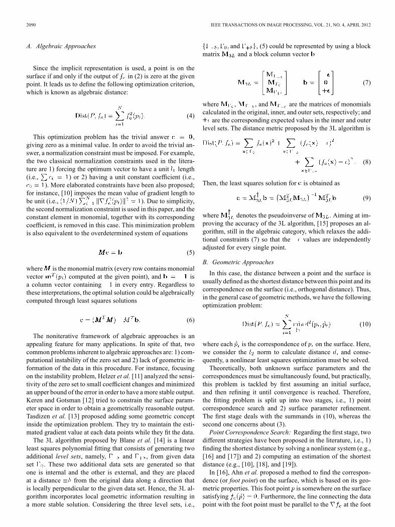
and , (5) could be represented by using a blockmatrix and a block column vector
(7)
where , , and are the matrices of monomialscalculated in the original, inner, and outer sets, respectively; andare the corresponding expected values in the inner and outer
level sets. The distance metric proposed by the 3L algorithm is
(8)
Then, the least squares solution for is obtained as
(9)
where denotes the pseudoinverse of . Aiming at im-proving the accuracy of the 3L algorithm, [15] proposes an al-gorithm, still in the algebraic category, which relaxes the addi-tional constraints (7) so that the values are independentlyadjusted for every single point.
B. Geometric Approaches
In this case, the distance between a point and the surface isusually defined as the shortest distance between this point and itscorrespondence on the surface (i.e., orthogonal distance). Thus,in the general case of geometric methods, we have the followingoptimization problem:
(10)
where each is the correspondence of on the surface. Here,we consider the norm to calculate distance , and conse-quently, a nonlinear least squares optimization must be solved.Theoretically, both unknown surface parameters and the
correspondences must be simultaneously found, but practically,this problem is tackled by first assuming an initial surface,and then refining it until convergence is reached. Therefore,the fitting problem is split up into two stages, i.e., 1) pointcorrespondence search and 2) surface parameter refinement.The first stage deals with the summands in (10), whereas thesecond one concerns about (3).Point Correspondence Search: Regarding the first stage, two
different strategies have been proposed in the literature, i.e., 1)finding the shortest distance by solving a nonlinear system (e.g.,[16] and [17]) and 2) computing an estimation of the shortestdistance (e.g., [10], [18], and [19]).In [16], Ahn et al. proposed a method to find the correspon-
dence (or foot point) on the surface, which is based on its geo-metric properties. This foot point is somewhere on the surfacesatisfying . Furthermore, the line connecting the datapoint with the foot point must be parallel to the at the foot
ROUHANI AND SAPPA: IMPLICIT POLYNOMIAL REPRESENTATION THROUGH A FAST FITTING ERROR ESTIMATION 2091
point, where is the gradient operator. In other words, we musthave . Merging these two conditions, the fol-lowing system of equations must be solved:
(11)
This equation could be solved by the Newton–Rophson algo-rithm for nonlinear system of equations. Although the fittingmethod in [16] is precise enough, and even covers some well-known methods in the literature such as [10] and [20], it is quitetime consuming due to the iterations.In [17], the orthogonal fitting is extended for general error
functions such as the and norms of the residual error in-stead of the common norm. This highlights the importance ofthe error function selection for the fitting process. The authorspresent the fitting algorithm as an evolutionary process of a sur-face along its normal direction. They discuss and compare theirapproach with other common error functions, including the al-gebraic types.Instead of computing the shortest distance through (11), [19]
proposes approximating it, avoiding iterative approaches as aresult. In that work, which is an extension of [18] for moregeneral surfaces, first, a normal vector for each point iscomputed by using the principal component analysis in a small
neighborhood centered at each point [21]. In other words,is defined as the eigenvector of local co-
variance matrix associated with the smallest eigenvalue
(12)
where is the vector showing the mean po-sition of the neighboring points in the region. Finally,is computed as the intersection of the surface with aline passing through and parallel to , i.e.,
(13)
The intersection is used as an approximation for the foot pointin the geometric distance (10).In [10], Taubin proposes an approximation for (10), which is
based on the first-order Taylor expansion of the distance func-tion. The distance could be computed through normalizing thealgebraic distance by the gradient norm
(14)
This approximated distance is used in an iterative weighted leastsquares method and in a nonlinear optimization framework. Inaddition, a new constraint is imposed on the coefficient vector,which is based on the data points and on the coefficients. Theapproximated distance proposed by Taubin [10] may not reachthe correspondence point lying on the zero set, which could af-fect the final fitting result. In fact, instead of considering the zeroset, the level set where the point is lying on is affected by thisoptimization process. Finally, every point forces its level set tomove in order to reach a lower accumulated distance.
Fig. 1. Simplex used for estimating the geometric distance: (a) 2-D case and(b) 3-D case.
Surface Parameter Refinement: As a result from the previousstage, the set of points corresponding to every inthe given data set has been found. Afterward, it must be fol-lowed by an optimization framework to refine the surface pa-rameter. Although different optimization algorithms could beused (e.g., genetic algorithm (GA) [19], trust region [22], quasi-Newton method [23], and particle swarm [24]), in this paper,the LMA [25] has been chosen since it exploits gradient infor-mation provided by the proposed distance estimation. LMA, insome sense, interpolates between the Gauss–Newton algorithmand the gradient descent (more details about the LMA are givenin Section III-B).
III. PROPOSED APPROACH
This paper proposes a geometric approach to tackle IPs fit-ting through an estimation of the orthogonal distance. In spiteof being focused on the geometric framework, the polynomialcoefficients are first initialized by using an algebraic-based al-gorithm like the 3L algorithm [14]. This initialization processis intended for speeding up the convergence of the algorithm;other strategies, for instance, starting with the smallest boundingcircle/sphere, can be used as well. The proposed geometric ap-proach consists of two stages. First, the residual error from thegiven set of points to the initial IP coefficients is estimated bymeans of the proposed approach. Then, the IP coefficients areaccordingly updated through LMA. The two stages are repeateduntil convergence is reached; they are detailed next.
A. Approximated Residual Error
The first contribution of this paper lies in a direct approach toestimate the orthogonal distance, which works as follows. First,a simplex is constructed through each point and its intersectionsalong the coordinate axis. A simplex is a triangle in 2-D anda tetrahedron in 3-D, as depicted in Fig. 1(a) and (b), respec-tively. Without loss of generality, the 3-D case is consideredhere. In this case, having constructed the tetrahedron, its heightsegment is considered as an approximation of the geometric dis-tance. This tetrahedron is defined by the given point and threeintersections satisfying , ,and , where is the givenpoint. In the particular case tackled in this paper, since the fittedcurve/surface is defined by the implicit polynomial (1), the inter-secting points are found by computing the closest root of three1-D functions to the data point.Once the intersecting points have been obtained, a direct for-
mula is used to estimate the geometric distance. Let , , and
2092 IEEE TRANSACTIONS ON IMAGE PROCESSING, VOL. 21, NO. 4, APRIL 2012
Fig. 2. Contour of constant distance for (a) orthogonal distance; (b) algebraic distance; (c) [10]; and (d) proposed distance estimation.
be the three intersections with the current surface that create atriangular planar patch [see Fig. 1(b)]. Since the volume of thetetrahedron is defined as the product of the area of each base byits corresponding height, three sets of expressions lead us to thesame value. Hence, the height of the tetrahedron could beeasily computed from the following relationship:
(15)
where refers to the cross-product operator between two vec-tors. Similar relationship can be obtained in the 2-D case byusing the triangle area instead of the tetrahedron volume. Moredetails can be found in [9].As presented above, in order to estimate the distance, the in-
tersections of the curve/surface along the coordinate axis mustbe found first. In the quadric case, these intersections can be di-rectly found [9]. However, for higher degree cases, an iterativemethod should be used to find the roots. In the current imple-mentation, Newton’s method has been used [26]. In the casethat the first iteration is considered, an approximation of theroot can be obtained through the first-order Taylor expansion.For instance, the expansion along the axis can be expressedas follows:
(16)
where corresponds to the partial derivative in the -direction,and is the intersection of the surface with the line passingthrough in the -direction. Hence, segment can be easilyestimated as
(17)
Considering similar approximations for the other two intersec-tions, the proposed distance for point could be approximatedas follows:
(18)
thus, the proposed distance is a generalization of Taubin’smethod when the intersections are approximated.The preciseness of the proposed distance is presented for two
examples in Fig. 2 and compared with other approximated dis-tances, as well as with the orthogonal one. The first row of thefigure shows the isocontours1 of the set ,which consists of two intersecting lines, and the second rowshows the isocontours of a regular curve
. As illustrated in the last two columns, ourmethodand Taubin’s similarly behave in the linear case (when the Jaco-bian matrix is linear with respect to the point coordinates). In thesecond example, our method outperforms compared with otherapproximations and has a quite similar result to the isocontoursobtained by the orthogonal method.
B. Implicit Polynomial Fitting
As a result from the previous stage, the distance from eachsingle data point to the current curve/surface has been found.Accumulation of all these distances provides a good criterionfor curve surface fitting
(19)
1Contours with the same distance from the zero set.
ROUHANI AND SAPPA: IMPLICIT POLYNOMIAL REPRESENTATION THROUGH A FAST FITTING ERROR ESTIMATION 2093
This distance is in the least squares formwhere each term is non-linear with respect to coefficient vector . It provides a straight-forward method to approximate the orthogonal distance. Hence,it can be used in an appropriate optimization algorithm to findthe best parameters describing the given set of points. We al-ready used this distance in a RANdom SAmple Consensus-based framework to find the quadratic surface parameters [9].Other optimization techniques such as GA [19] or quasi-Newtonmethod [23] have been already used in surface fitting.This paper not only proposes a simple and fast distance es-
timation but also, as a second contribution, it shows how thisestimation can be used in a nonlinear framework. In our im-plementation, the LMA has been used [25] to optimize the dis-tance (19) with respect to the curve/surface parameters. LMA isspecifically designed for nonlinear functions in the least squaresform, which is the case in (19). It starts from an initial coefficientvector , obtained by some algebraic fitting technique (asaforementioned, the result from the 3L algorithm has been usedas initialization). LMA updates these parameters iteratively asfollows:
diag (20)
where is the refinement step; represents the refine-ment vector for the surface parameters; is the dampingparameter in LMA; is the Jacobian matrix of ; andvector corresponds to distances
, whose norm must be minimized. Pa-rameter refinement (20) must be repeated until convergencehappens.Each iteration of LMA contains two stages, namely, 1) dis-
tance estimation and 2) Jacobian matrix computation. In the firststage, all the intersections along the coordinate axis must befound. For this purpose, Newton’s method is applied to find theroot of the parametric function , which is a 1-D func-tionwith respect to . Direction vector is set to ,
, and for each axis. Having com-puted all the intersections along the coordinate axis, the terms
, , and , and consequently the distance (15), can beestimated. As aforementioned, it should be noticed here that ifwe stop the Newton’s method after one iteration, the proposeddistance will be easily computed through (18), which is the sameas [10].In order to handle LMA, the value of the functional (19) and
its partial derivatives, which are used to build the Jacobian ma-trix, should be provided. These values show the sensitivity ofeach in (15) with respect to parameter vector . The Jacobianmatrix could be directly derived through the differentiation rulesas follows:
(21)
where is the differentiation operator with respect toparameters. Since the intersection , , and lies on the surface,
, , , and can be implicitly expressed as afunction of the surface parameters. In order to calculate each
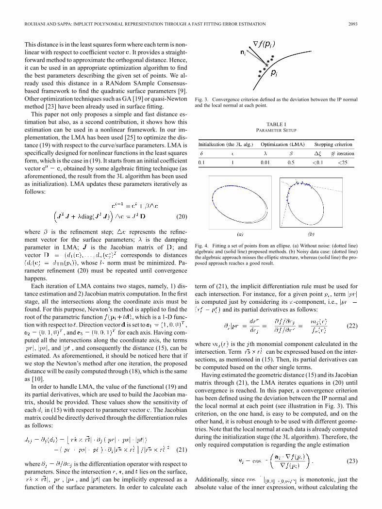
Fig. 3. Convergence criterion defined as the deviation between the IP normaland the local normal at each point.
TABLE IPARAMETER SETUP
Fig. 4. Fitting a set of points from an ellipse. (a) Without noise: (dotted line)algebraic and (solid line) proposed methods. (b) Noisy data case: (dotted line)the algebraic approach misses the elliptic structure, whereas (solid line) the pro-posed approach reaches a good result.
term of (21), the implicit differentiation rule must be used foreach intersection. For instance, for a given point , termis computed just by considering its -component, i.e.,
and its partial derivatives as follows:
(22)
where is the th monomial component calculated in theintersection. Term can be expressed based on the inter-sections, as mentioned in (15). Then, its partial derivatives canbe computed based on the other single terms.Having estimated the geometric distance (15) and its Jacobian
matrix through (21), the LMA iterates equations in (20) untilconvergence is reached. In this paper, a convergence criterionhas been defined using the deviation between the IP normal andthe local normal at each point (see illustration in Fig. 3). Thiscriterion, on the one hand, is easy to be computed, and on theother hand, it is robust enough to be used with different geome-tries. Note that the local normal at each data is already computedduring the initialization stage (the 3L algorithm). Therefore, theonly required computation is regarding the angle estimation
(23)
Additionally, since is monotonic, just theabsolute value of the inner expression, without calculating the
2094 IEEE TRANSACTIONS ON IMAGE PROCESSING, VOL. 21, NO. 4, APRIL 2012
Fig. 5. Two-dimensional contours fitted by (first and second rows) fifth- and (third, fourth, and fifth rows) sixth-degree IPs’ results from (a) 3L algorithm, (b)[10], (c) proposed approach, and (d) [16], which is used as a ground truth. AFE shows the accumulated fitting errors. The fourth row shows a case where [16] stopsdue to the maximum iteration criterion.
cosine inverse, is considered. Therefore, the criterion used formeasuring the goodness of the current fitting result is
(24)
where is the number of points in the original data set. LMAiterates while (24) decreases more than a user-defined threshold
or a maximum number of iterations is reached.
IV. EXPERIMENTAL RESULTS
The proposed method, which belongs to the geometric fittingcategory, is implemented and compared with the most importantmethods in the literature, both algebraic and geometric. The re-sults presented here are evaluated using the fitting error (FE)computed for every single points with [16]. It is used to ob-tain a quantitative criterion for comparison, which is referred to
Fig. 6. Fitting two concentric ellipses. (a) Result from the 3L algorithm.(b) Result from the proposed approach.
as accumulated FE (AFE) where AFE FE . In all thecases, the given data points are centralized and scaled between
. The parameters of initialization (3L algorithm), opti-mization (LMA), and stopping criterion are empirically set up,
ROUHANI AND SAPPA: IMPLICIT POLYNOMIAL REPRESENTATION THROUGH A FAST FITTING ERROR ESTIMATION 2095
Fig. 7. Synthetic data sets fitted with the proposed approach.
as presented in Table I. The same initialization and stopping cri-terion have been used once the proposed approach is comparedwith other approaches.In the 2-D case, different sets of points picked from quadric
contours sampled with nonuniform distributions have beenfitted with the proposed approach and compared with otherapproaches. Fig. 4(a) depicts the result of the proposed methodwhen a nonuniformly distributed 2-D data set is fitted. Boththe algebraic and proposed methods converge to a similarresult, but problems arise when noise is added to the points.Fig. 4(b) highlights the robustness of the proposed method tonoise, whereas the algebraic one misses the elliptic structureof the data and fits the patch as a split hyperbola. Fitzgibbonet al. [27] propose a fitting method just for 2-D elliptic casesbased on algebraic approaches. From this simple example, onecan understand the hardship for algebraic methods when thefunction space is bigger than the quadratic one.The proposed approach is also implemented for fitting higher
degree IPs. Fig. 5 shows 2-D contours fitted by fifth- and sixth-degree IPs (depending on the shape complexity) using the 3Lalgorithm [see Fig. 5(a)], the approach proposed in [10] [seeFig. 5(b)], the proposed approach [see Fig. 5(c)], and a nonlinearorthogonal-distance-based approach [16] used as a ground truth[see Fig. 5(d)]. The fitting error, computed over the whole setof points with [16], is used as a quantitative criterion for com-parison. In all the cases, the accuracy obtained with the pro-posed approach considerably improves the one obtained withthe 3L algorithm and, in most of the cases, gives better resultsthan [10]; it is comparable (in one case better since the stoppingcriterion has been reached, see fourth row) to the results ob-tained when the nonlinear approach is used. Although out of thescope of this paper, it should be mentioned that in the 2-D case,the proposed approach is about 10 times faster than [16]. Fi-nally, another challenging 2-D shape defined by two concentricellipses has been fitted by a fifth-degree IP using the proposed
TABLE IISYNTHETIC DATA SET: AFE CORRESPONDING TO THE ILLUSTRATIONS
PRESENTED IN Fig. 7
Fig. 8. Solid surface representing a fourth-degree IP; wire frame is used tovisualize given data points. (a) IP obtained from the 3L algorithm. (b) Resultfrom the proposed approach (note the similarity between the wire frame and thesurface from the computed IP).
approach; Fig. 6(a) shows the result from the 3L algorithm usedas initialization of the proposed approach. The final result is de-picted in Fig. 6(b).The proposed approach has been also evaluated with 3-D data
sets, i.e., both synthetic and real data sets were fitted with low-and high-degree IPs. On average, in the 3-D case, the proposedapproach is not as good as in the 2-D case, but it is about twicefaster than [16]. Fig. 7 shows eight different results obtainedwith the proposed approach; in all the cases, the results are quite
2096 IEEE TRANSACTIONS ON IMAGE PROCESSING, VOL. 21, NO. 4, APRIL 2012
Fig. 9. Data set from AIM@SHAPE fitted with the proposed approach.
Fig. 10. (a) Fitting with a rough initialization. (b)–(d) First, second, and thirditerations, respectively.
TABLE IIIDATA SET FROM AIM@SHAPE: AFE CORRESPONDING TO THE
ILLUSTRATIONS PRESENTED IN FIG. 9
similar to the ones obtained with [16] and considerably betterthan those obtained with [14]. Table II presents the AFE ob-tained with the different approaches for a quantitative compar-
ison. Note that these results were obtained once the stoppingcriterion has been reached; if a larger number of iterations areallowed, [16] achieves better results. The proposed algorithmhas been tested with a more challenging 3-D data set with a dif-ferent topology; Fig. 8 presents the results from both the 3L al-gorithm AFE , which is used as an initialization of theproposed approach, and the final result obtained after ten itera-tions AFE . In this case, a fourth-degree IP hasbeen used (solid surface), given that data points are representedby means of a wire frame just for a visual comparison.In addition to the synthetic objects, a data set from
AIM@SHAPE2 has been used for evaluating the proposedapproach. Fig. 9 shows eight illustrations of fourth-, sixth-,and seventh-degree IPs obtained with the proposed approach.Table III presents the AFE obtained with the different ap-proaches for a quantitative comparison. Fig. 10 illustrates theindependence to initial guess by using a sphere covering thegiven data set as an initialization [see Fig. 10(a)]. The first,second, and third iterations of the proposed approach are shownin Fig. 10(b)–(d), respectively; the result obtained after 25iterations is already depicted in Fig. 9(a). Surface parameterrefinements through these iterations are depicted in Fig. 11.Fig. 11(a) corresponds to the evolution of the 35 IP coefficients,whereas Fig. 11(b) shows how the AFE decreases with theiterations. Finally, Fig. 11(c) depicts the accumulated angle(23) used as a convergence criterion. It should be mentionedthat this criterion has a similar behavior than Fig. 11(b), but itscomplexity is considerably lower.
V. CONCLUSION
This paper has presented a novel geometric approach for2-D/3-D implicit polynomial fitting, which is based on a fastgeometric distance estimation. Despite other geometric esti-mations, which are based on a single direction to find the foot
2http://shapes.aimatshape.net/
ROUHANI AND SAPPA: IMPLICIT POLYNOMIAL REPRESENTATION THROUGH A FAST FITTING ERROR ESTIMATION 2097
Fig. 11. Parameter evolution of Fig. 10 along 25 iterations: (a) IP coefficient values, (b) AFE, and (c) accumulated angle used as a convergence criterion.
point associated to each data point, the proposed one is basedon two or three directions (depending on the data dimension).The smoothness and accuracy of the proposed distance havebeen shown. Additionally, the implicit connection betweenthis distance and the IP coefficients has been presented andshown to be differentiable. This property allows the use ofany gradient-based optimization techniques. In this paper, theLMA is applied to find the best set of surface parameters in aniterative way. Comparisons with state-of-the-art techniques arepresented. Moreover, the proposed distance is proved to be ageneralization of the distance presented in [10].
ACKNOWLEDGMENT
The authors would like to thank the Associate Editor andthe anonymous referees for their valuable and constructivecomments.
REFERENCES
[1] M. Sarkis and K. Diepold, “Content adaptive mesh representation ofimages using binary space partitions,” IEEE Trans. Image Process.,vol. 18, no. 5, pp. 1069–1079, May 2009.
[2] A. Jalba and J. Roerdink, “Efficient surface reconstruction from noisydata using regularized membrane potentials,” IEEE Trans. ImageProcess., vol. 18, no. 5, pp. 1119–1134, May 2009.
[3] C. Darolti, A. Mertins, C. Bodensteiner, and U. Hofmann, “Local re-gion descriptors for active contours evolution,” IEEE Trans. ImageProcess., vol. 17, no. 12, pp. 2275–2288, Dec. 2008.
[4] V. Srikrishnan and S. Chaudhuri, “Stabilization of parametric activecontours using a tangential redistribution term,” IEEE Trans. ImageProcess., vol. 18, no. 8, pp. 1859–1872, Aug. 2009.
[5] H. Ben-Yaacov, D. Malah, and M. Barzohar, “Recognition of 3-D ob-jects based on implicit polynomials,” IEEE Trans. Pattern Anal. Mach.Intell., vol. 32, no. 5, pp. 954–960, May 2010.
[6] B. Zheng, J. Takamatsu, and K. Ikeuchi, “An adaptive and stablemethod for fitting implicit polynomial curves and surface,” IEEETrans. Pattern Anal. Mach. Intell., vol. 32, no. 3, pp. 561–568, Mar.2010.
[7] R. Xu and M. Kemp, “Fitting multiple connected ellipses to an imagesilhouette hierarchically,” IEEE Trans. Image Process., vol. 19, no. 7,pp. 1673–1682, Jul. 2010.
[8] M. Rouhani and A. D. Sappa, “A novel approach to geometric fittingof implicit quadrics,” in Proc. 11th Int. Conf. Adv. Concepts Intell. Vis.Syst., Bordeaux, France, Sep. 28–Oct., 2 2009, pp. 121–132.
[9] A. Sappa and M. Rouhani, “Efficient distance estimation for fitting im-plicit quadric surfaces,” inProc. IEEE Int. Conf. Image Process., Cairo,Egypt, Nov. 2009, pp. 3521–3524.
[10] G. Taubin, “Estimation of planar curves, surfaces, and nonplanar spacecurves defined by implicit equations with applications to edge andrange image segmentation,” IEEE Trans. Pattern Anal. Mach. Intell.,vol. 13, no. 11, pp. 1115–1138, Nov. 1991.
[11] A. Helzer, M. Barzohar, and D. Malah, “Stable fitting of 2-D curvesand 3-D surfaces by implicit polynomials,” IEEE Trans. Pattern Anal.Mach. Intell., vol. 26, no. 10, pp. 1283–1294, Oct. 2004.
[12] D. Keren and C. Gotsman, “Fitting curves and surfaces with con-strained implicit polynomials,” IEEE Trans. Pattern Anal. Mach.Intell., vol. 21, no. 1, pp. 476–480, Jan. 1999.
[13] T. Tasdizen, J. Tarel, and D. Cooper, “Improving the stability of alge-braic curves for applications,” IEEE Trans. Image Process., vol. 9, no.3, pp. 405–416, Mar. 2000.
[14] M. Blane, Z. Lei, H. Civil, and D. Cooper, “The 3L algorithm for fittingimplicit polynomials curves and surface to data,” IEEE Trans. PatternAnal. Mach. Intell., vol. 22, no. 3, pp. 298–313, Mar. 2000.
[15] M. Rouhani and A. D. Sappa, “Relaxing the 3L algorithm for an accu-rate implicit polynomial fitting,” in Proc. IEEE Int. Conf. Comput. Vis.Pattern Recog., San Francisco, CA, Jun. 2010, pp. 3066–3072.
[16] S. Ahn, W. Rauh, H. Cho, and H. Warnecke, “Orthogonal distance fit-ting of implicit curves and surfaces,” IEEE Trans. Pattern Anal. Mach.Intell., vol. 24, no. 5, pp. 620–638, May 2002.
[17] M. Aigner and B. Jütler, “Gauss–Newton-type technique for robustlyfitting implicit defined curves and surfaces to unorganized data points,”in Proc. IEEE Int. Conf. Shape Model. Appl., New York, Jun. 2009, pp.121–130.
[18] Y. Chen and C. Liu, “Quadric surface extraction using genetic algo-rithms,” Comput.-Aided Des., vol. 31, no. 2, pp. 101–110, Feb. 1999.
[19] P. Gotardo, O. Bellon, K. Boyer, and L. Silva, “Range image segmen-tation into planar and quadric surfaces using an improved robust es-timator and genetic algorithm,” IEEE Trans. Syst., Man, Cybern. B,Cybern., vol. 34, no. 6, pp. 2303–2316, Dec. 2004.
[20] P. D. Sampson, “Fitting conic sections to very scattered data: An iter-ative refinement of the Bookstein algorithm,” Comput. Graph. ImageProcess., vol. 18, no. 1, pp. 97–108, Jan. 1982.
[21] H. Hoppe, T. DeRose, T. Duchamp, J. A. McDonald, and W. Stuetzle,“Surface reconstruction from unorganized points,” in Proc. 19th Annu.Conf. Comput. Graph. Interactive Techn., SIGGRAPH, Chicago, IL,Jul. 1992, pp. 71–78.
[22] H. Helfrich and D. Zwick, “A trust region algorithm for parametriccurve and surface fitting,” J. Comput. Appl. Math., vol. 73, no. 1/2, pp.119–134, Oct. 1996.
[23] W. Wang, H. Pottmann, and Y. Liu, “Fitting B-spline curves to pointclouds by curvature-based squared distance minimization,” ACMTrans. Graph., vol. 25, no. 2, pp. 214–238, Apr. 2006.
[24] D. Adi, S. Shamsuddin, and A. Ali, “Particle swarm optimization fornurbs curve fitting,” in Proc. IEEE Int. Conf. Comput. Graph., Imag.Vis., Tianjin, China, Aug. 2009, pp. 259–263.
[25] R. Fletcher, Practical Methods of Optimization, 2nd ed. New York:Wiley, 1990.
[26] J. Stoer and R. Bulirsch, Introduction to Numerical Analysis, 3rd ed.New York: Springer-Verlag, 2002.
[27] A. Fitzgibbon, M. Pilu, and R. Fisher, “Direct least square fitting ofellipses,” IEEE Trans. Pattern Anal. Mach. Intell., vol. 21, no. 5, pp.476–480, May 1999.
2098 IEEE TRANSACTIONS ON IMAGE PROCESSING, VOL. 21, NO. 4, APRIL 2012
Mohammad Rouhani (S’09) received the Bach-elor’s degree in applied mathematics from theNational University of Iran (currently Shahid Be-heshti University), Tehran, Iran, in 2003 and theMaster’s degree from Sharif University of Tech-nology, Tehran, in 2006. He is currently workingtoward the Ph.D. in computer vision at the ComputerVision Center, Barcelona, Spain.Before studying for the Ph.D. degree, he spent two
years in lecturing at Shomal University, Amol, Iran.His research is jointly on 3-D computer vision and
computer graphics, including 2-D/3-D shape modeling, reconstruction, and reg-istration.Mr. Rouhani is a member of the Advanced Driver Assistance Systems Group,
Computer Vision Center.
Angel Domingo Sappa (S’94–M’00) received theelectromechanical engineering degree from theNational University of La Pampa, General Pico,Argentina, in 1995 and the Ph.D. degree in industrialengineering from the Polytechnic University ofCatalonia, Barcelona, Spain, in 1999.In 2003, after holding research positions in
France, U.K., and Greece, he joined the ComputerVision Center, Barcelona, where he is currently aSenior Researcher. His current research focuses onstereo image processing and analysis, 3-D modeling,
and dense optical flow estimation. His research interests span a broad spectrumwithin the 2-D and 3-D image processing.Dr. Sappa is a member of the Advanced Driver Assistance Systems Group,