Catching Objects in FlightSeungsu Kim, Ashwini Shukla, and Aude Billard
Abstract—We address the difficult problem of catching in-flightobjects with uneven shapes. This requires the solution of threecomplex problems: accurate prediction of the trajectory of fast-moving objects, predicting the feasible catching configuration, andplanning the arm motion, and all within milliseconds. We follow aprogramming-by-demonstration approach in order to learn, fromthrowing examples, models of the object dynamics and arm move-ment. We propose a new methodology to find a feasible catchingconfiguration in a probabilistic manner. We use the dynamicalsystems approach to encode motion from several demonstrations.This enables a rapid and reactive adaptation of the arm motionin the presence of sensor uncertainty. We validate the approach insimulation with the iCub humanoid robot and in real-world exper-iments with the KUKA LWR 4+ (7-degree-of-freedom arm robot)to catch a hammer, a tennis racket, an empty bottle, a partiallyfilled bottle, and a cardboard box.
Index Terms—Catching, Gaussian mixture model, machinelearning, robot control, support vector machines.
I. INTRODUCTION
W E consider the problem of catching fast-flying objectson nonballistic flight trajectories: in flights that last less
than a second, with objects that have arbitrary shapes and mass,and when the catching point is not located at the center ofmass (COM). The latter condition requires the robot to adopt aparticular orientation of the arm to catch the object at a specificpoint (e.g., catching the lower part of the handle of a hammer).
Catching such an object in-flight is extremely challenging andrequires the solution to three complex problems.
1) accurate prediction of the trajectory of the objects: the factthat an arbitrary shaped or nonrigid object yields a highlynonlinear translational and rotational motion of the object;
2) predicting the optimal catching configuration (interceptpoint): As the robot must catch the object with a particu-lar hand orientation, this limits tremendously the possiblecatching configurations;
3) fast planning of precise trajectories for the robot’s arm tointercept and catch the object on time, given that the objectis in-flight for less than a second.
Manuscript received January 31, 2014; revised March 17, 2014; acceptedMarch 22, 2014. This paper was recommended for publication by AssociateEditor E. Marchand and Editor D. Fox upon evaluation of the reviewers’ com-ments. This work was supported by the EU Projects AMARSI (FP7-ICT-248311)and FirstMM (FP7-248258).
This paper has supplementary downloadable material available athttp://ieeexplore.ieee.org, provided by the authors.
Color versions of one or more of the figures in this paper are available onlineat http://ieeexplore.ieee.org.
Digital Object Identifier 10.1109/TRO.2014.2316022
Fig. 1. Schematic overview of the system.
Accurate prediction of the flight trajectory of the object relieson accurate sensing, which cannot always be ensured in robotics.This requires a frequent reestimation of the target’s location asboth robot and object move. To compensate for such inaccu-rate sensing, we need to predict robustly the whole trajectoryof fast-moving objects against sensor noise and external pertur-bations. At the same time, we need to constantly and rapidlyrepredict a feasible catching configuration and regenerate thedesired trajectory of the robot’s arm. A schematic overview ofour framework is shown in Fig. 1.
A. Robotic Catching
A body of work has been devoted to the autonomous control offast movements such as catching [13], [18], [25], [28], [30]–[32],[44], hitting flying objects [24], [37], and juggling [6], [33], [35].We here briefly review these works with a focus on how they 1)predict trajectories of moving objects, 2) determine the catchingposture, and 3) generate desired trajectories for the robot’s armand hand.
1) Object Trajectory Prediction: To catch effectively a mov-ing object, we must predict its trajectory ahead of time. This thenserves to determine the catching point along this trajectory. Mostapproaches assume a known model of the dynamics of motion.For instance, Hong and Slotine [18] and Riley and Atkeson [32]model the trajectory of a flying ball as a parabola and estimatethe parameters of the model recursively through least squaresoptimization. Frese et al. [13] use a ballistic model incorporatedwith air drag for the ball trajectories; they use it in conjunctionwith an extended Kalman filter (EKF) [3] for online reestimationof the trajectory.
Such approaches are accurate at estimating the trajectories,but they rely on an analytical motion model for the object. Inaddition, most of the study is tuned for spherical objects byestimating only the position of the object’s COM. However, to
catch a complex object such as a hammer or a tennis racket, weneed to estimate the complete pose of the object to determine theprecise location of the grasping posture. This grasping postureis usually not located on the COM of the object.1 Rigid bodydynamics [5] can be applied to estimate the complete pose ofthe object but still requires the properties of the object to bemeasured (such as its mass, position of the COM, and momentof inertia).
In our previous work [22], we learned from demonstrationsthe dynamics of more complex objects whose shapes are arbi-trary, nonrigid, or their points of interest are not at the COM. Weencode the demonstrations using a dynamical system (DS) thatprovides an efficient way to model the dynamics of a movingobject, solely by observing examples of the object’s motion inspace. Note that this does not require any prior information onthe physical properties of the object, such as its mass, positionof COM, and moment of inertia. In order to deal with noise andunseen perturbations, we combine the output of the regressionmodel of the machine-learning techniques with EKF. Once thesystem is learned from the demonstrations, it is used to predictthe object acceleration and angular acceleration at each step intime given an observed current position, velocity, orientation,and angular velocity of the object. We estimate the whole tra-jectory of the object by integrating these values further in time.It is noted that the estimates are in the 6-D space (position of thepoint of interest and an orientation of a frame rigidly attachedto the object). In this paper, we further develop the previouswork by combining it with an algorithm to accurately predictthe grasping posture of the hand. Next, we review the state ofthe art to determine the catching configuration.
2) Catching Pose Prediction: One way to determine the de-sired catching posture is to determine the intersection betweenthe robot’s reachable space (usually its boundary is representedas a series of spheres or planes) and the object’s trajectory. Ifthere is more than one solution, one chooses the intersectionpoint that is closest to either the robot’s base [18] or to theinitial position of the end-effector [13]. Although this methodworks well to determine the location of the catching point, itdoes not determine the orientation of the object because theseworks only consider ball-shaped objects. Furthermore, these ap-proaches give a coarse approximation of the robot’s reachablespace in Cartesian space by limiting the radius and height of arobot [18] or using an infinite polyhedron [13].
3) Planning Catching Motion: The final catching configu-ration is constantly updated at a very fast rate to counter unseendynamic effects. From a control viewpoint, this requires therobot motion planner to be very rapid (of the order of 10 ms) inreplanning the desired trajectory as the position of the catchingpoint keeps changing (as an effect of reestimating the trajectoryof the object). Moreover, for efficient catching, in addition tothe end-effector motion, the dynamics of the fingers need tobe properly tuned to avoid the object bouncing off the palm orfingers.
To represent the desired trajectory for the end-effector incatching tasks, many researchers [18], [30], [37], [44] use poly-
1In our experiments, the grasping points are represented by a constant trans-formation from the user-defined measurement frame of the object.
nomials that satisfy boundary values. For instance, Namiki andIshikawa [30] minimize the sum of the torques and angular ve-locities to satisfy constraints on the initial and final position,velocity, and acceleration of the end-effector. Note here that,although all of these approaches were successfully applied toobject catching, hitting, or juggling, they were explicitly timedependent; hence, any temporal perturbation after the onset ofthe motion was not properly handled.
Spline-based trajectory generation [1], [19] and minimum-jerk [27] methods have also been popular means to encode time-indexed trajectories with a finite set of terminal constraints, e.g.,positions, velocities, and accelerations at start and end points.However, the number of control points and degrees of the splineneed to be tuned depending on the nonlinearity of the motions.Moreover, as the constraints are only terminal, it is difficult toestablish the feasibility of the state space (position-orientationtuples) visited because of interpolation. One way to alleviatethis problem is to directly model trajectories in joint space. Thiswould require a fast and global inverse kinematics (IK) solver. Itis difficult to obtain an IK solver without heuristics for generalkinematic chains. Furthermore, it is hard to learn a global IKsolver from human demonstrations because of the redundancyand singularities of the human and robot work spaces.
Another approach for generating end-effector trajectoriesuses human demonstrations to learn generalized descriptionsof a skill. To catch vertically falling objects, Riley et al. [32]use point-to-point motion primitives that are learned using pro-grammable pattern generators [34] based on human movements.Their approach is capable of modifying the trajectory online fora new target. Our work follows this line of research and fur-ther develops controllers to guide hand–arm motion, which islearned from human demonstration.
In our recent work [14], [20], we take the approaches ofusing time-invariant DSs as a method for encoding robotmotion. We showed that this could be applied to various tasksthat require rapid and precise recomputation of the end-effectormotion, such as obstacle avoidance [21]. The drawback of usingtime-invariant controllers is that one does not control explicitlyfor time. When catching an object in flight, controlling for timeis crucial. In [23], we offered a solution to control for the taskduration in time-invariant DS controller, through fast-forwardintegration and scaling. Even though many approaches mightbe valid for the robotic catching task, we follow our previousapproach here to enable the robot to intercept the flying object ata particular time and particular posture by boosting the learneddynamics. One of the advantages of this approach is that weexpect that the trajectory generated by the learned model is fea-sible, as the approach uses feasible demonstrations to train themodel. Furthermore, for the frequent changes of predicted catch-ing posture, our method provides a way of adapting the robotmotion to these changes by expecting the feasibility [14], [20].
Another aspect of object catching that is inadequately or notat all addressed by the aforementioned works is the motion ofthe fingers. To complete the catch, the dynamics of the fingermotion need to be appropriately tuned and coupled to the armmotion.
Most works on catching depend on the very rapid closing ofthe fingers. Usually, finger closure is triggered once the distance
KIM et al.: CATCHING OBJECTS IN FLIGHT 3
between the object and the end-effector has decreased below acertain threshold [18], [28], [30], [32]. This approach requiresthe precise tuning of several parameters including the threshold,the finger trajectory, and velocity. Bauml et al. [4] present anoptimization-based approach that minimizes the accelerationof robot’s joints during the catching. Although this method isvery effective, it requires significant computing power in theform of 32-core parallel programming to compute the optimizedsolution at run time. In our previous work on ball catching[23], we simply perform a linear interpolation between the restposition and grasping configuration of the fingers, depending onthe distance of the ball from the palm.
In [38], we show that modeling arm and hand motion throughcoupled dynamical systems (CDS) is advantageous over theclassic approaches reviewed previously. The explicit couplingbetween arm and hand dynamics ensures that the finger closurewill be naturally triggered at the right time, even when the handmotion is delayed or accelerated to adapt to changes in theprediction of the catching point. This offers a robust and fastcontrol of the complete hand–arm system without resorting toextensive parameter tuning.
B. Reachable Space Modeling
Representing the space of the robot’s feasible hand posturesis essential for both catching the object and for planning the armmotion. Before initiating the arm movement for catching, weneed to calculate if any graspable part of the object lies insidethe reachable space.
Early investigations of this issue focus on determining andgenerating a geometrical model of the reachable space of therobot. Polynomial discriminants [43] and classic geometric ap-proaches [29], [26] are used to characterize the boundaries ofthe robot’s reachable space. However, these methods cover onlya few special kinematic chains and are not applicable to allmanipulators.
Another body of approaches approximates the reachablespace of a robot as density functions [9], [40]. These proveto be useful for dealing with large datasets of reachable end-effector positions. However, these methods are evaluated onlyfor discretely actuated manipulators. Detry et al. [11] introducea method to model a graspable space by using a density func-tion approach. They model the 6-D graspable space by usingkernel density function. The model is learned by letting a robotto explore successful grasping postures. Our study is similar tothat of Detry et al. [11] in that we also model the graspablespace. Additionally, we model the reachable space and proposea means by which we can combine the two probabilistic repre-sentations. To ensure finding the best grasping posture in realtime, combining the two (reachable space and graspable space)models is essential in our application.
More recent approaches target the creation of full databasesof the reachable positions obtained by sampling the Cartesianspace Guilamo et al. [17] use a database of mapping betweenthe joint angles of a robot and the discrete voxel representationof the reachable space. Guan and Yokoi [16] also propose adatabase approach to represent the reachable space for a full-
body humanoid robot. Three-dimensional reachable space isdiscretely divided into cells, and while the robot ensures properbalancing, it tests each cell to check the reachability. All thesuccessful configurations are then stored in the database. Inanother work, the same authors [15] propose a mathematicalmethod to model the boundary of the reachable space, whilethe robot ensures kinematic constraints and proper balancing.However, these methods yield a discrete approximation of thereachable space without a precise description of the boundary.Moreover, these are expressed as only 3-D positions in Cartesianspace.
A few works consider the orientation to model the reachablespace of a robot. Zacharias et al. [41], [42] propose a compactrepresentation of the Cartesian reachable space. They uniformlydivide the complete reachable space into 3-D cells. Then, theybuild a capability map that represents how many orientations arereachable at each position cell. However, this map is discreteand only gives a score that reflects the ease of reaching to thatposition. Similarly, DianKov et al. [12] store all the valid 6-Dend-effector positions by randomly sampling the 6-D poses andsolving IK for each of these.
The reachable space depends on the number of degreesof freedom (DOF) of a robot, joint limits, link lengths, self-collision, etc. Hence, the 6-D reachable space, which is spannedby the feasible positions and orientations of a robot, is highlynonlinear and varies drastically from robot to robot. Here, wepropose a probabilistic model of the 6-D reachable space of therobot hand (all feasible positions and orientations).
C. Our Approaches and Contributions
In this paper, we propose a framework that enables a robot tocatch flying objects. We combine three strands of our previousworks on 1) learning how to predict accurately the trajectory offast-moving objects [22], 2) learning hand–finger coordinatedmotion [38], and 3) controlling the timing of motion when con-trolled with DSs [23].
Additionally, we propose a new approach for modeling thereachable space of the robot arm and for modeling the graspablespace of an object, in order to determine the optimal catchingconfiguration. We also exploit the probabilistic nature of thismodel to query conditional information (e.g., given a position,we can query the best orientation). Finally, this paper proposesa novel approach for learning how to determine the mid-flightcatching configuration (intercept point).
The experimental validation of this study in which a robotcatches in-flight objects with uneven mass distribution (seeSection III) is, in our view, the core contribution of this study.We believe that it significantly advances the field, in offeringan example of ultrafast control in the face of uncertainty. Al-though in the past, the field has seen impressive examples ofobject catching in-flight, they were either restricted to catch-ing simple spherical objects [13], [28], [30]–[32], [44] or tocatching objects with a slow changing orientation (e.g., a paperairplane [18]). The speed of computation in the experiments wepresent here is not the mere effect of having more rapid comput-ing facilities than available in the past; it also benefits from the
4 IEEE TRANSACTIONS ON ROBOTICS
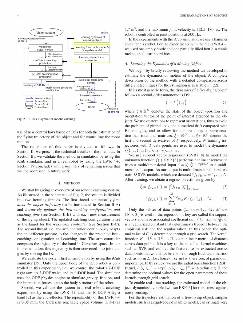
Fig. 2. Block diagram for robotic catching.
use of new control laws based on DSs for both the estimation ofthe flying trajectory of the object and for controlling the robotmotion.
The remainder of this paper is divided as follows. InSection II, we present the technical details of the methods. InSection III, we validate the method in simulation by using theiCub simulator, and in a real robot by using the LWR 4+.Section IV concludes with a summary of remaining issues thatwill be addressed in future work.
II. METHODS
We start by giving an overview of our robotic catching system.As illustrated in the schematic of Fig. 2, the system is dividedinto two iterating threads. The first thread continuously pre-dicts the object trajectory (to be introduced in Section II-A)and iteratively updates the best-catching configuration andcatching time (see Section II-B) with each new measurementof the flying object. The updated catching configuration is setas the target for the robot-arm controller (see Section II-C).The second thread, i.e., the arm controller, continuously adaptsthe end-effector posture to the changes in the predicted best-catching configuration and catching time. The arm controllercomputes the trajectory of the hand in Cartesian space. In ourimplementation, this trajectory is then converted into joint an-gles by solving the IK.
We evaluate the system first in simulation by using the iCubsimulator [39]. Only the upper body of the iCub robot is con-trolled in this experiment, i.e., we control the robot’s 7-DOFright arm, its 3-DOF waist, and its 9-DOF hand. The simulatoruses the ODE physics engine to simulate gravity, friction, andthe interaction forces across the body structure of the robot.
Second, we validate the system in a real robotic catchingexperiment by using the LWR 4+ and the 16-DOF Allegrohand [2] as the end-effector. The repeatability of this LWR 4+is 0.05 mm, the Cartesian reachable space volume in 3-D is
1.7 m3 , and the maximum joint velocity is 112.5–180 ◦/s. Therobot is controlled in joint positions at 500 Hz.
In the experiments with the iCub simulator, we use a hammerand a tennis racket. For the experiments with the real LWR 4+,we used one empty bottle and one partially filled bottle, a tennisracket, and a cardboard box.
A. Learning the Dynamics of a Moving Object
We begin by briefly reviewing the method we developed toestimate the dynamics of motion of the object. A completedescription of the method with a detailed comparison acrossdifferent techniques for the estimation is available in [22].
In its most generic form, the dynamics of a free-flying objectfollows a second-order autonomous DS:
ξ̈ = f(ξ, ξ̇
)(1)
where ξ ∈ RD denotes the state of the object (position andorientation vector of the point of interest attached to the ob-ject). We use quaternions to represent orientations, thus to avoidthe problem of gimbal lock and numerical drift compared withEuler angles, and to allow for a more compact representa-tion than rotational matrices. ξ̇ ∈ RD and ξ̈ ∈ RD denote thefirst and second derivatives of ξ, respectively. N training tra-jectories with T data points are used to model the dynamics{{ξt,n , ξ̇t,n , ξ̈t,n}t=1...T }n=1...N .
We use support vector regression (SVR) [8] to model theunknown function f(.). SVR [8] performs nonlinear regressionfrom a multidimensional input ζ = [ξ; ξ̇] ∈ R2×D to a unidi-mensional output. As our output is multidimensional, here, wetrain D SVR models, which are denoted dfSVR , d = 1, . . . , D.After training, we obtain a regression estimate given by
ξ̈ = fSVR (ζ) =[dfSVR (ζ)
]d=1...D
(2)
dfSVR (ζ) =M∑
m=1
dαm K(ζ, dζm
)+ db. (3)
Only the subset of data points ζm , m = 1 . . . M , M <=(N × T ) is used in the regression. They are called the supportvectors and have associated coefficient αm �= 0, |αm | < C
M . Cis a regularized constant that determines a tradeoff between theempirical risk and the regularization. In this paper, the opti-mal value of C is determined through a grid search. The kernelfunction K : RD ×RD → R is a nonlinear metric of distanceacross data points. It is a key to the so-called kernel machinessuch as SVR and enables the features to be extracted acrossdata points that would not be visible through Euclidian metrics,such as norm 2. The choice of kernel is, therefore, of paramountimportance. In this study, we use the radial basis function (RBF)kernel, K(ζ, ζm ) = exp(−γ‖ζ − ζm‖2) with radius γ ∈ R anddetermine the optimal values for the open parameters of thesekernels through grid search.
To enable real-time tracking, the estimated model of the ob-jects dynamics is coupled with an EKF [3] for robustness againstnoisy sensing.
For the trajectory estimation of a free-flying object, simplermodels, such as a rigid-body dynamics model, can estimate very
KIM et al.: CATCHING OBJECTS IN FLIGHT 5
accurately the trajectory. However, these techniques usually re-quire modeling all the forces acting on the object and measuringproperties of the object, such as its mass, position of COM, mo-ment of inertia, shape, and size. Measuring these values forarbitrary objects (such as a bottle, racket, or a cardboard box) isnot a trivial problem. Furthermore, these properties might noteven be constant and may change during flight (as it is the casewith a partially filled bottle). The machine-learning approachwe follow in this paper avoids gathering such a priori informa-tion on the object and estimates directly the nonlinear dynamicsof the object’s flight from observing several examples of suchtrajectories [22].
B. Predicting the Catching Configuration
We now turn to the problem of determining where to catch theobject. As mentioned in Section I, the problem is particularlydifficult when we aim at catching the object with a particulargrasping configuration. In this case, we must proceed in threesteps. 1) First, we must determine how to grasp the object. Forthis, we show several demonstrations of various grasps on theconsidered object, and we learn a distribution of possible handpositions and orientations. 2) Second, we must determine thereachable space of the robot that is the possible positions andorientations the robot’s hand can achieve. 3) Finally, we mustdetermine a point along the object trajectory for which we canfind a feasible posture of the robot’s hand [using the solutionto problem (2)], which will yield a possible grasp [using thesolution to problem (1)]. Next, we describe how we achieveeach of these three steps.
We define η = [ηpos ; ηori ] as the catching configuration,where ηpos ∈ R3 denotes the end-effector position, and ηori ∈R6 denotes the orientation that is composed of the firsttwo column vectors of the corresponding rotation matrixrepresentation.
The way we represent orientation (ηori) requires more di-mensions than the Euler angle or quaternion representation. Ex-pressing orientation by using the rotation matrix, however, hasseveral benefits. First, we can easily rotate the trained Gaussianmodel in real time by simply multiplying the original modelwith the rotation matrix, as will be described in Section II-B1.This is highly advantageous for catching tasks that require rapidcomputation. Furthermore, the rotation matrix representation isunambiguous and singularity free. It can also represent the sim-ilarity between orientations more accurately than Euler angle orquaternion representation. For instance, the Euclidean distancebetween the quaternions q and −q is large; however, the actualorientation is the same. This is important as the closeness be-tween postures is exploited in our probabilistic model to queryfor regions encapsulating close and feasible postures.
1) Graspable-Space Model: To acquire a series of possi-ble grasping positions and orientations for a given robot hand,we perform grasping demonstrations by passively driving therobot’s hand joint close on the object. We put markers on boththe object and the robot hand. Using our motion capture sys-tem, we record a series of grasping postures by changing the
positions and orientations of the object and the robot hand. Thegrasping postures are stored in the object coordinate system.
We model the density distribution of these positions andorientations using the Gaussian mixture model (GMM) [7].The trained graspable-space model, objMgrasp composed ofK Gaussians, is represented as obj{πk , μk ,Σk}k=1:K . obj de-notes the coordinate frame in which the data and the Gaussiansare represented. πk , μk , and Σk are the parameters of kth Gaus-sian and correspond to the prior, mean, and covariance matrix,respectively. These parameters are calculated using expectationmaximization [10]. The probability density of a given graspingconfiguration η ∈ R9 for the graspable-space model is given by
P (η|Mgrasp) =K∑
k=1
πkN (η|μk ,Σk ) . (4)
A given configuration η is said to be feasible (i.e., it willyield a successful grasp) when P (η|Mgrasp) exceeds a gras-pable likelihood threshold ρgrasp . The threshold is determinedsuch that the likelihoods of 99% of grasping demonstrations arehigher than the threshold. The number of Gaussians K is deter-mined using the Bayesian information criterion (BIC) [36]. Twosets of grasping demonstrations and their graspable probabilitycontour are shown in Figs. 3, 4, 18, and 19.
The likelihood is a measure of the density of feasible graspsin the immediate vicinity. It represents a measure of fitness of aregion for grasping. High density (likelihood) in a region resultsfrom the fact that this region was more frequently explored byhumans; hence, it has a high probability of being a successfulgrasping location, whereas less- dense regions (likelihood lessthan a threshold) are bad regions to grasp, as they are rarelyseen in the demonstrations. The graspability in these regions isknown with much less certainty.
As the graspable-space model of the object is expressed inthe object reference frame and the object moves, we provide asimple way of changing the reference frame of the model to therobot’s reference frame by using the following transformation:
Here, p (t) ∈ R3 and R (t) ∈ R3×3 are the position vectorand orientation matrix of the object reference frame (measure-ment frame) with respect to the robot’s base reference frame;Ω(t) = diag (R(t), R(t), R(t)) is a 9 × 9 matrix whose diag-onal entries are R(t); zeros(6, 1) represents 6 × 1 zero vector.For convenience, we will skip the superscript robot. Note that inall our experiments, the robot is fixed at the hip, i.e., the robot’sbase reference frame does not move.
2) Reachable-Space Model: In order to choose a catchingconfiguration, the robot needs to know that the graspable partof the object is in a reachable space, before initiating thearm movement. To model the reachable space, we simulate all
6 IEEE TRANSACTIONS ON ROBOTICS
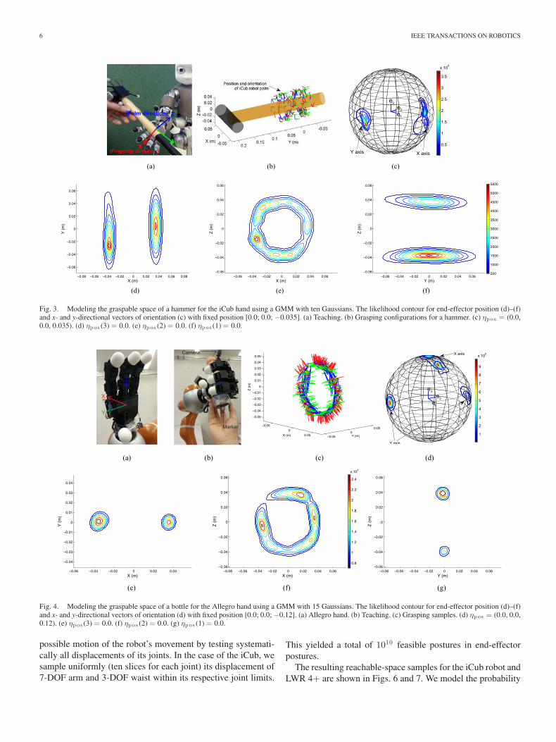
Fig. 3. Modeling the graspable space of a hammer for the iCub hand using a GMM with ten Gaussians. The likelihood contour for end-effector position (d)–(f)and x- and y-directional vectors of orientation (c) with fixed position [0.0; 0.0; −0.035]. (a) Teaching. (b) Grasping configurations for a hammer. (c) ηpos = (0.0,0.0, 0.035). (d) ηpos (3) = 0.0. (e) ηpos (2) = 0.0. (f) ηpos (1) = 0.0.
Fig. 4. Modeling the graspable space of a bottle for the Allegro hand using a GMM with 15 Gaussians. The likelihood contour for end-effector position (d)–(f)and x- and y-directional vectors of orientation (d) with fixed position [0.0; 0.0; −0.12]. (a) Allegro hand. (b) Teaching. (c) Grasping samples. (d) ηpos = (0.0, 0.0,0.12). (e) ηpos (3) = 0.0. (f) ηpos (2) = 0.0. (g) ηpos (1) = 0.0.
possible motion of the robot’s movement by testing systemati-cally all displacements of its joints. In the case of the iCub, wesample uniformly (ten slices for each joint) its displacement of7-DOF arm and 3-DOF waist within its respective joint limits.
This yielded a total of 1010 feasible postures in end-effectorpostures.
The resulting reachable-space samples for the iCub robot andLWR 4+ are shown in Figs. 6 and 7. We model the probability
KIM et al.: CATCHING OBJECTS IN FLIGHT 7
Fig. 5. BIC curves to model the graspable-space models. We determine thenumber of Gaussians as 10 for the graspable-space model of a hummer (a) and15, 13, 14, for the graspable-space model of a bottel, a tennis racket, and acardboard box, respectively (b). (a) A hammer for iCub hand. (b) For Allegrohand.
distribution of these positions and orientations using GMMsMreach , {πl, μl ,Σl}l=1:L . Similarly to what was performed forthe graspable-space model, we compute the likelihood of anygiven pose being reachable.
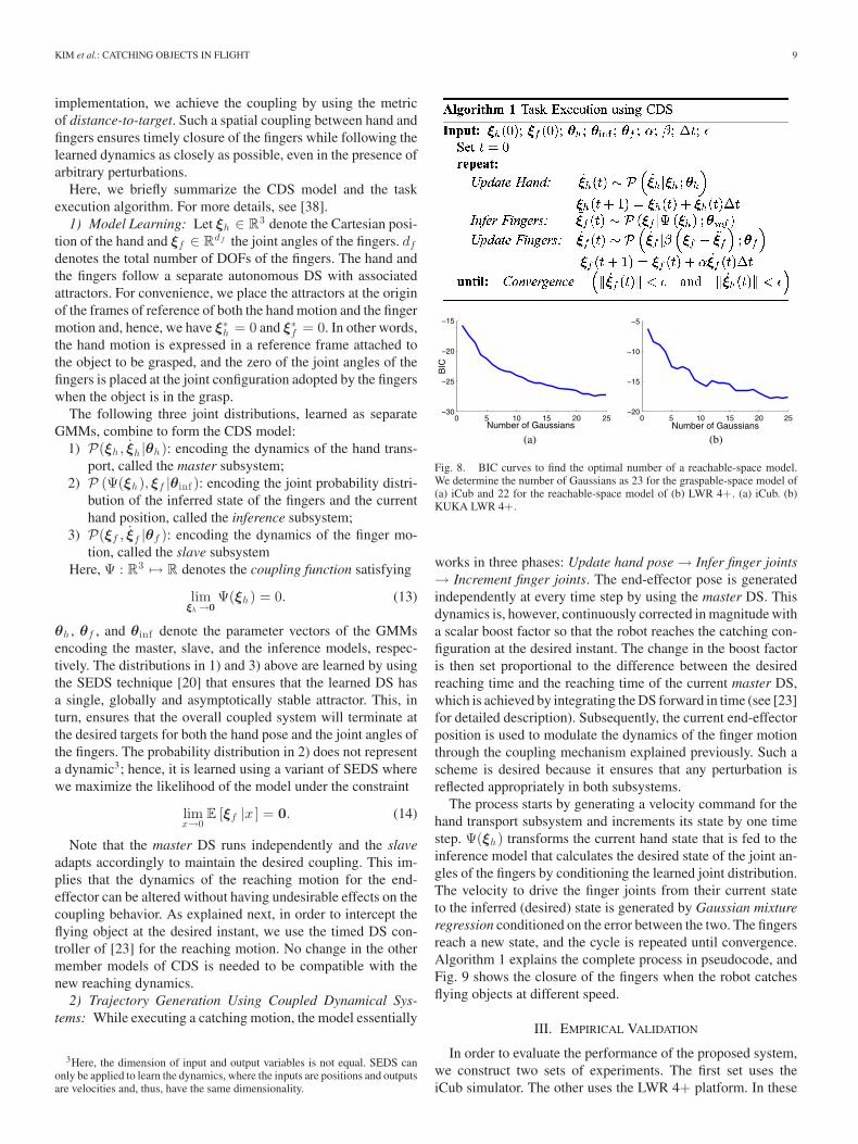
The optimal numbers of Gaussians for the reachable-spacemodel of the iCub and LWR 4+ are determined using BIC [36].Their BIC curves are shown in Fig. 8. Based on this analysis,the number of Gaussians we determined is 23 for the reachable-space model of the iCub, and 22 for the LWR 4+. To verify theaccuracy of the reachable-space models, we randomly sample1 million joint configurations within the joint limits for eachrobot and evaluate them. Only 0.12% (for iCub) and 0.13% (forLWR 4+) of samples fell outside the estimated reachable space.
In this specific catching experiment with LWR, we discard thereachable samples that are in a condition of z < 0.1 m. This en-sures that the robot avoids collision with the table whose surfaceis the plane z = 0. To build a self-collision-free reachable-spacemodel, we conservatively limit the joint ranges. Furthermore, wealso discard the reachable samples in which the palm directionis facing toward the ground. Using this way, we discard theundesirable postures without using any heuristics at runtime.
By embedding the set of reachable postures in a probabil-ity density function, we directly check if a target end-effectorposture is reachable, which saves computational time duringexecution.
3) Predicting Catching Configuration: The graspable-spaceand reachable-space models explained previously are statisti-cally independent. Hence, we can calculate their joint probabil-ity distribution by simply multiplying the distributions. The jointmodel M(t)joint , {π(t)j , μ(t)j ,Σ(t)j}j=1:J , has J = K × Lnumber of Gaussians. Each of the J Gaussians are expressed as
Σ(t)j =(Σ(t)k
−1 + Σl−1
)−1(8)
μ(t)j = Σ(t)jΣ(t)k−1μ(t)k + Σ(t)jΣl
−1μl (9)
π(t)j =π(t)k
ηgrasp· πl
ηreach· N (μ(t)k |μl,Σ(t)k + Σl) (10)
where j = (l − 1) × L + k.In order to find the optimal catching configuration η(t)
at a predicted object pose (at a time slice of the pre-dicted trajectory), we use the joint model M(t)joint of
graspable-space and reachable-space models. We computearg maxη (t) P(η(t)|M(t)joint), through gradient ascent on thejoint model. The Jacobian of this objective function is given by
∂P(η(t)|M(t)joint
)
∂η(t)=
−J∑
j=1
π(t)jΣ(t)j−1
(η(t) − μ(t)j
)N
(η(t)|μ(t)j ,Σ(t)j
).
(11)
We initialize the gradient ascent with the center μ(t)j of theGaussian that is closest to the current hand pose (Euclideandistance in 6-D), and we solve this optimization problem. Theoutput of the optimization is a hand pose that has the highestlikelihood at the time slice. We compute this for each timeslice until the predicted end of flight. The optimal catchingconfiguration and catching time is the configuration and timeslice with the highest likelihood. Each time we receive a newmeasurement of the object’s current pose, we again predict thetrajectory and repeat the procedure described previously.
The lengths of the resultant two directional vectors in η(t)oriare not exactly 1. At each step of the gradient ascent method,we normalize the vectors and orthogonalize them so that theresulting rotation matrix is orthonormal. Theoretically, this isa modeling inaccuracy, but because of the reprojection steponto the set of valid rotation matrices, we get a suboptimal butfeasible solution.
To reduce the risk that the hand enters in collision with theobject, we make sure that the direction of the palm in the catch-ing configuration is opposite from the direction of the objectvelocity.2 This is achieved by requiring the dot product betweenthe direction of the robot’s palm and the negative velocity of theobject to be greater than a threshold as the below constraint:
dot(η̇(t)pos , η(t)palm
)< d (12)
where η(t)palm is a palm direction vector [for LWR with AllegroHand, the palm direction is −η(t)ori,x , see Fig. 4(a)]. d is adirection difference threshold constant. In our experiment, dwas set as 0.5, which allows for 60.0◦ direction difference. Thisheuristic constraint greatly decreases the chance of a collisionbetween the robot hand (on the back or side) and the object.
The predicted end-effector pose is mapped into the attractorof the DS-based controller that drives the hand toward the target,and the predicted catching time is set as the desired reachingtime in the timing controller [23], as we will explain in the nextsection.
2Because of the rapid nature of this task, it is not possible to detect andhandle the collisions in real time as this would require an additional optimizationsubroutine in the control loop. Performing fast and reactive obstacle avoidancein full configuration space, while adhering to the timing constraints of the task,is an open and difficult problem. In place of doing explicit collision avoidance,we use a heuristic to avoid collisions between the robot fingers and the flyingobjects. When we determine the best catching posture, we make sure that thepalm direction in the catching configuration is opposite from the direction ofthe object velocity.
8 IEEE TRANSACTIONS ON ROBOTICS
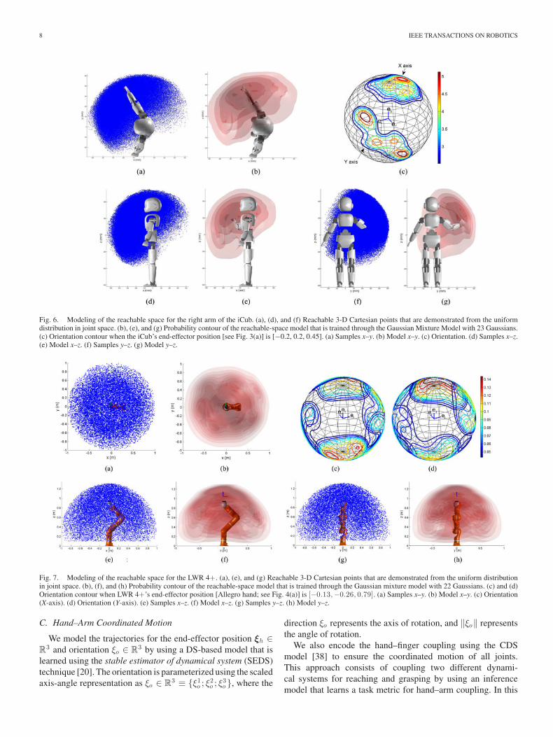
Fig. 6. Modeling of the reachable space for the right arm of the iCub. (a), (d), and (f) Reachable 3-D Cartesian points that are demonstrated from the uniformdistribution in joint space. (b), (e), and (g) Probability contour of the reachable-space model that is trained through the Gaussian Mixture Model with 23 Gaussians.(c) Orientation contour when the iCub’s end-effector position [see Fig. 3(a)] is [−0.2, 0.2, 0.45]. (a) Samples x–y. (b) Model x–y. (c) Orientation. (d) Samples x–z.(e) Model x–z. (f) Samples y–z. (g) Model y–z.
Fig. 7. Modeling of the reachable space for the LWR 4+. (a), (e), and (g) Reachable 3-D Cartesian points that are demonstrated from the uniform distributionin joint space. (b), (f), and (h) Probability contour of the reachable-space model that is trained through the Gaussian mixture model with 22 Gaussians. (c) and (d)Orientation contour when LWR 4+’s end-effector position [Allegro hand; see Fig. 4(a)] is [−0.13,−0.26, 0.79]. (a) Samples x–y. (b) Model x–y. (c) Orientation(X-axis). (d) Orientation (Y-axis). (e) Samples x–z. (f) Model x–z. (g) Samples y–z. (h) Model y–z.
C. Hand–Arm Coordinated Motion
We model the trajectories for the end-effector position ξh ∈R3 and orientation ξo ∈ R3 by using a DS-based model that islearned using the stable estimator of dynamical system (SEDS)technique [20]. The orientation is parameterized using the scaledaxis-angle representation as ξo ∈ R3 ≡ {ξ1
o ; ξ2o ; ξ3
o }, where the
direction ξo represents the axis of rotation, and ‖ξo‖ representsthe angle of rotation.
We also encode the hand–finger coupling using the CDSmodel [38] to ensure the coordinated motion of all joints.This approach consists of coupling two different dynami-cal systems for reaching and grasping by using an inferencemodel that learns a task metric for hand–arm coupling. In this
KIM et al.: CATCHING OBJECTS IN FLIGHT 9
implementation, we achieve the coupling by using the metricof distance-to-target. Such a spatial coupling between hand andfingers ensures timely closure of the fingers while following thelearned dynamics as closely as possible, even in the presence ofarbitrary perturbations.
Here, we briefly summarize the CDS model and the taskexecution algorithm. For more details, see [38].
1) Model Learning: Let ξh ∈ R3 denote the Cartesian posi-tion of the hand and ξf ∈ Rdf the joint angles of the fingers. df
denotes the total number of DOFs of the fingers. The hand andthe fingers follow a separate autonomous DS with associatedattractors. For convenience, we place the attractors at the originof the frames of reference of both the hand motion and the fingermotion and, hence, we have ξ∗
h = 0 and ξ∗f = 0. In other words,
the hand motion is expressed in a reference frame attached tothe object to be grasped, and the zero of the joint angles of thefingers is placed at the joint configuration adopted by the fingerswhen the object is in the grasp.
The following three joint distributions, learned as separateGMMs, combine to form the CDS model:
1) P(ξh , ξ̇h |θh): encoding the dynamics of the hand trans-port, called the master subsystem;
2) P (Ψ(ξh), ξf |θinf ): encoding the joint probability distri-bution of the inferred state of the fingers and the currenthand position, called the inference subsystem;
3) P(ξf , ξ̇f |θf ): encoding the dynamics of the finger mo-tion, called the slave subsystem
Here, Ψ : R3 → R denotes the coupling function satisfying
limξh →0
Ψ(ξh) = 0. (13)
θh , θf , and θinf denote the parameter vectors of the GMMsencoding the master, slave, and the inference models, respec-tively. The distributions in 1) and 3) above are learned by usingthe SEDS technique [20] that ensures that the learned DS hasa single, globally and asymptotically stable attractor. This, inturn, ensures that the overall coupled system will terminate atthe desired targets for both the hand pose and the joint angles ofthe fingers. The probability distribution in 2) does not representa dynamic3; hence, it is learned using a variant of SEDS wherewe maximize the likelihood of the model under the constraint
limx→0
E [ξf |x ] = 0. (14)
Note that the master DS runs independently and the slaveadapts accordingly to maintain the desired coupling. This im-plies that the dynamics of the reaching motion for the end-effector can be altered without having undesirable effects on thecoupling behavior. As explained next, in order to intercept theflying object at the desired instant, we use the timed DS con-troller of [23] for the reaching motion. No change in the othermember models of CDS is needed to be compatible with thenew reaching dynamics.
2) Trajectory Generation Using Coupled Dynamical Sys-tems: While executing a catching motion, the model essentially
3Here, the dimension of input and output variables is not equal. SEDS canonly be applied to learn the dynamics, where the inputs are positions and outputsare velocities and, thus, have the same dimensionality.
Fig. 8. BIC curves to find the optimal number of a reachable-space model.We determine the number of Gaussians as 23 for the graspable-space model of(a) iCub and 22 for the reachable-space model of (b) LWR 4+. (a) iCub. (b)KUKA LWR 4+.
works in three phases: Update hand pose → Infer finger joints→ Increment finger joints. The end-effector pose is generatedindependently at every time step by using the master DS. Thisdynamics is, however, continuously corrected in magnitude witha scalar boost factor so that the robot reaches the catching con-figuration at the desired instant. The change in the boost factoris then set proportional to the difference between the desiredreaching time and the reaching time of the current master DS,which is achieved by integrating the DS forward in time (see [23]for detailed description). Subsequently, the current end-effectorposition is used to modulate the dynamics of the finger motionthrough the coupling mechanism explained previously. Such ascheme is desired because it ensures that any perturbation isreflected appropriately in both subsystems.
The process starts by generating a velocity command for thehand transport subsystem and increments its state by one timestep. Ψ(ξh) transforms the current hand state that is fed to theinference model that calculates the desired state of the joint an-gles of the fingers by conditioning the learned joint distribution.The velocity to drive the finger joints from their current stateto the inferred (desired) state is generated by Gaussian mixtureregression conditioned on the error between the two. The fingersreach a new state, and the cycle is repeated until convergence.Algorithm 1 explains the complete process in pseudocode, andFig. 9 shows the closure of the fingers when the robot catchesflying objects at different speed.
III. EMPIRICAL VALIDATION
In order to evaluate the performance of the proposed system,we construct two sets of experiments. The first set uses theiCub simulator. The other uses the LWR 4+ platform. In these
10 IEEE TRANSACTIONS ON ROBOTICS
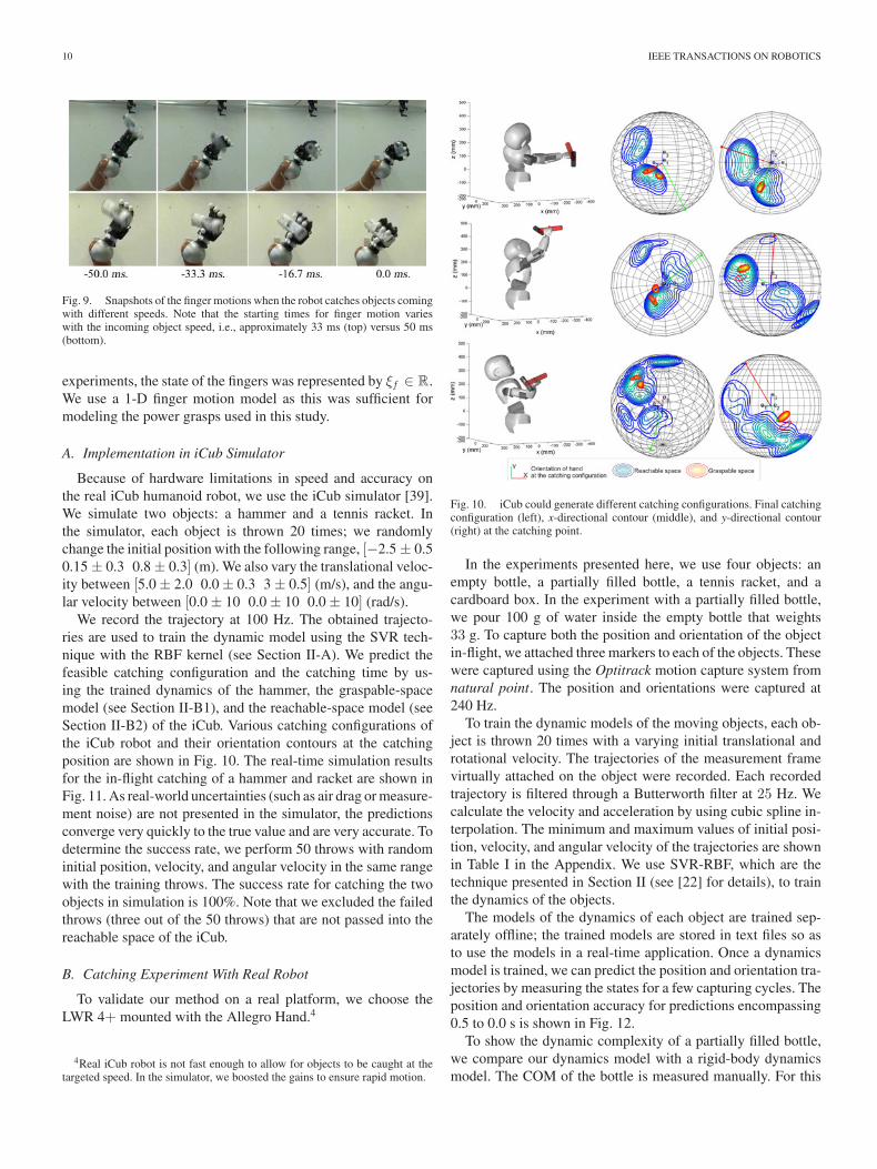
Fig. 9. Snapshots of the finger motions when the robot catches objects comingwith different speeds. Note that the starting times for finger motion varieswith the incoming object speed, i.e., approximately 33 ms (top) versus 50 ms(bottom).
experiments, the state of the fingers was represented by ξf ∈ R.We use a 1-D finger motion model as this was sufficient formodeling the power grasps used in this study.
A. Implementation in iCub Simulator
Because of hardware limitations in speed and accuracy onthe real iCub humanoid robot, we use the iCub simulator [39].We simulate two objects: a hammer and a tennis racket. Inthe simulator, each object is thrown 20 times; we randomlychange the initial position with the following range, [−2.5 ± 0.50.15 ± 0.3 0.8 ± 0.3] (m). We also vary the translational veloc-ity between [5.0 ± 2.0 0.0 ± 0.3 3 ± 0.5] (m/s), and the angu-lar velocity between [0.0 ± 10 0.0 ± 10 0.0 ± 10] (rad/s).
We record the trajectory at 100 Hz. The obtained trajecto-ries are used to train the dynamic model using the SVR tech-nique with the RBF kernel (see Section II-A). We predict thefeasible catching configuration and the catching time by us-ing the trained dynamics of the hammer, the graspable-spacemodel (see Section II-B1), and the reachable-space model (seeSection II-B2) of the iCub. Various catching configurations ofthe iCub robot and their orientation contours at the catchingposition are shown in Fig. 10. The real-time simulation resultsfor the in-flight catching of a hammer and racket are shown inFig. 11. As real-world uncertainties (such as air drag or measure-ment noise) are not presented in the simulator, the predictionsconverge very quickly to the true value and are very accurate. Todetermine the success rate, we perform 50 throws with randominitial position, velocity, and angular velocity in the same rangewith the training throws. The success rate for catching the twoobjects in simulation is 100%. Note that we excluded the failedthrows (three out of the 50 throws) that are not passed into thereachable space of the iCub.
B. Catching Experiment With Real Robot
To validate our method on a real platform, we choose theLWR 4+ mounted with the Allegro Hand.4
4Real iCub robot is not fast enough to allow for objects to be caught at thetargeted speed. In the simulator, we boosted the gains to ensure rapid motion.
Fig. 10. iCub could generate different catching configurations. Final catchingconfiguration (left), x-directional contour (middle), and y-directional contour(right) at the catching point.
In the experiments presented here, we use four objects: anempty bottle, a partially filled bottle, a tennis racket, and acardboard box. In the experiment with a partially filled bottle,we pour 100 g of water inside the empty bottle that weights33 g. To capture both the position and orientation of the objectin-flight, we attached three markers to each of the objects. Thesewere captured using the Optitrack motion capture system fromnatural point. The position and orientations were captured at240 Hz.
To train the dynamic models of the moving objects, each ob-ject is thrown 20 times with a varying initial translational androtational velocity. The trajectories of the measurement framevirtually attached on the object were recorded. Each recordedtrajectory is filtered through a Butterworth filter at 25 Hz. Wecalculate the velocity and acceleration by using cubic spline in-terpolation. The minimum and maximum values of initial posi-tion, velocity, and angular velocity of the trajectories are shownin Table I in the Appendix. We use SVR-RBF, which are thetechnique presented in Section II (see [22] for details), to trainthe dynamics of the objects.
The models of the dynamics of each object are trained sep-arately offline; the trained models are stored in text files so asto use the models in a real-time application. Once a dynamicsmodel is trained, we can predict the position and orientation tra-jectories by measuring the states for a few capturing cycles. Theposition and orientation accuracy for predictions encompassing0.5 to 0.0 s is shown in Fig. 12.
To show the dynamic complexity of a partially filled bottle,we compare our dynamics model with a rigid-body dynamicsmodel. The COM of the bottle is measured manually. For this
KIM et al.: CATCHING OBJECTS IN FLIGHT 11
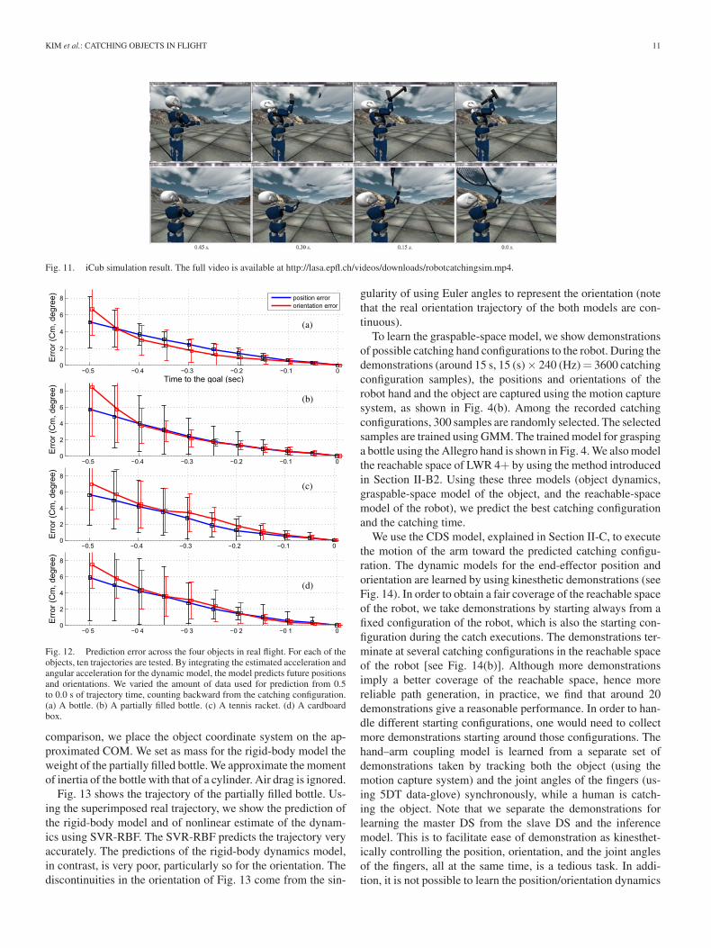
Fig. 11. iCub simulation result. The full video is available at http://lasa.epfl.ch/videos/downloads/robotcatchingsim.mp4.
Fig. 12. Prediction error across the four objects in real flight. For each of theobjects, ten trajectories are tested. By integrating the estimated acceleration andangular acceleration for the dynamic model, the model predicts future positionsand orientations. We varied the amount of data used for prediction from 0.5to 0.0 s of trajectory time, counting backward from the catching configuration.(a) A bottle. (b) A partially filled bottle. (c) A tennis racket. (d) A cardboardbox.
comparison, we place the object coordinate system on the ap-proximated COM. We set as mass for the rigid-body model theweight of the partially filled bottle. We approximate the momentof inertia of the bottle with that of a cylinder. Air drag is ignored.
Fig. 13 shows the trajectory of the partially filled bottle. Us-ing the superimposed real trajectory, we show the prediction ofthe rigid-body model and of nonlinear estimate of the dynam-ics using SVR-RBF. The SVR-RBF predicts the trajectory veryaccurately. The predictions of the rigid-body dynamics model,in contrast, is very poor, particularly so for the orientation. Thediscontinuities in the orientation of Fig. 13 come from the sin-
gularity of using Euler angles to represent the orientation (notethat the real orientation trajectory of the both models are con-tinuous).
To learn the graspable-space model, we show demonstrationsof possible catching hand configurations to the robot. During thedemonstrations (around 15 s, 15 (s)× 240 (Hz) = 3600 catchingconfiguration samples), the positions and orientations of therobot hand and the object are captured using the motion capturesystem, as shown in Fig. 4(b). Among the recorded catchingconfigurations, 300 samples are randomly selected. The selectedsamples are trained using GMM. The trained model for graspinga bottle using the Allegro hand is shown in Fig. 4. We also modelthe reachable space of LWR 4+ by using the method introducedin Section II-B2. Using these three models (object dynamics,graspable-space model of the object, and the reachable-spacemodel of the robot), we predict the best catching configurationand the catching time.
We use the CDS model, explained in Section II-C, to executethe motion of the arm toward the predicted catching configu-ration. The dynamic models for the end-effector position andorientation are learned by using kinesthetic demonstrations (seeFig. 14). In order to obtain a fair coverage of the reachable spaceof the robot, we take demonstrations by starting always from afixed configuration of the robot, which is also the starting con-figuration during the catch executions. The demonstrations ter-minate at several catching configurations in the reachable spaceof the robot [see Fig. 14(b)]. Although more demonstrationsimply a better coverage of the reachable space, hence morereliable path generation, in practice, we find that around 20demonstrations give a reasonable performance. In order to han-dle different starting configurations, one would need to collectmore demonstrations starting around those configurations. Thehand–arm coupling model is learned from a separate set ofdemonstrations taken by tracking both the object (using themotion capture system) and the joint angles of the fingers (us-ing 5DT data-glove) synchronously, while a human is catch-ing the object. Note that we separate the demonstrations forlearning the master DS from the slave DS and the inferencemodel. This is to facilitate ease of demonstration as kinesthet-ically controlling the position, orientation, and the joint anglesof the fingers, all at the same time, is a tedious task. In addi-tion, it is not possible to learn the position/orientation dynamics
12 IEEE TRANSACTIONS ON ROBOTICS
Fig. 13. Trajectory of a partially filled bottle and its prediction by using trained SVR-RBF dynamics model and rigid-body dynamics model. (a) Position.(b) Orientation.
Fig. 14. (a) Kinesthetic demonstrations of catching an object. (c) We track the hand and object using the marker-based OptiTrack system. The finger joint anglesare recorded synchronously for learning the hand–finger coupling. (d) Human catching the object while the hand position, object position, and finger joint anglesare recorded simultaneously.
Fig. 15. (a)–(d) Member models of the CDS used to control the Barrett Hand and KUKA LWR arm in coordination to execute the catching motions.(e)–(g) Orientation dynamics estimated using the SEDS technique.
solely using the latter procedure [see Fig. 14(d)], as this wouldrequire a remapping of the human data to the nonanthropomor-phic LWR arm. Fig. 15 shows the learned member models ofthe CDS formulation, i.e., the end-effector position representedby ξh ∈ R3 ≡ {ξ1
h ; ξ2h ; ξ3
h}, the state of the fingers representedby ξf ∈ R, and the DS encoding the orientation trajectories inthe scaled axis-angle representation ξo ∈ R3 ≡ {ξ1
o ; ξ2o ; ξ3
o }.
The predicted catching configuration, calculated by the abovebest catching configuration prediction module, is fed as thetarget for the position and orientation DSs. The fingers arecontrolled as the slave subsystem coordinated with the end-effector position with respect to the predicted catching config-uration. The end-effector and finger joint trajectories generatedby our model adapt to the predicted catching configuration that is
KIM et al.: CATCHING OBJECTS IN FLIGHT 13
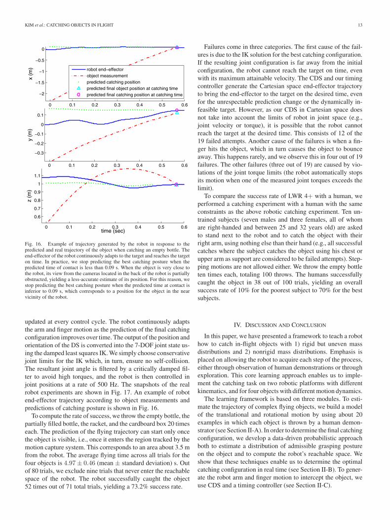
Fig. 16. Example of trajectory generated by the robot in response to thepredicted and real trajectory of the object when catching an empty bottle. Theend-effector of the robot continuously adapts to the target and reaches the targeton time. In practice, we stop predicting the best catching posture when thepredicted time of contact is less than 0.09 s. When the object is very close tothe robot, its view from the cameras located in the back of the robot is partiallyobstructed, yielding a less-accurate estimate of its position. For this reason, westop predicting the best catching posture when the predicted time at contact isinferior to 0.09 s, which corresponds to a position for the object in the nearvicinity of the robot.
updated at every control cycle. The robot continuously adaptsthe arm and finger motion as the prediction of the final catchingconfiguration improves over time. The output of the position andorientation of the DS is converted into the 7-DOF joint state us-ing the damped least squares IK. We simply choose conservativejoint limits for the IK which, in turn, ensure no self-collision.The resultant joint angle is filtered by a critically damped fil-ter to avoid high torques, and the robot is then controlled injoint positions at a rate of 500 Hz. The snapshots of the realrobot experiments are shown in Fig. 17. An example of robotend-effector trajectory according to object measurements andpredictions of catching posture is shown in Fig. 16.
To compute the rate of success, we throw the empty bottle, thepartially filled bottle, the racket, and the cardboard box 20 timeseach. The prediction of the flying trajectory can start only oncethe object is visible, i.e., once it enters the region tracked by themotion capture system. This corresponds to an area about 3.5 mfrom the robot. The average flying time across all trials for thefour objects is 4.97 ± 0.46 (mean ± standard deviation) s. Outof 80 trials, we exclude nine trials that never enter the reachablespace of the robot. The robot successfully caught the object52 times out of 71 total trials, yielding a 73.2% success rate.
Failures come in three categories. The first cause of the fail-ures is due to the IK solution for the best catching configuration.If the resulting joint configuration is far away from the initialconfiguration, the robot cannot reach the target on time, evenwith its maximum attainable velocity. The CDS and our timingcontroller generate the Cartesian space end-effector trajectoryto bring the end-effector to the target on the desired time, evenfor the unrespectable prediction change or the dynamically in-feasible target. However, as our CDS in Cartesian space doesnot take into account the limits of robot in joint space (e.g.,joint velocity or torque), it is possible that the robot cannotreach the target at the desired time. This consists of 12 of the19 failed attempts. Another cause of the failures is when a fin-ger hits the object, which in turn causes the object to bounceaway. This happens rarely, and we observe this in four out of 19failures. The other failures (three out of 19) are caused by vio-lations of the joint torque limits (the robot automatically stopsits motion when one of the measured joint torques exceeds thelimit).
To compare the success rate of LWR 4+ with a human, weperformed a catching experiment with a human with the sameconstraints as the above robotic catching experiment. Ten un-trained subjects (seven males and three females, all of whomare right-handed and between 25 and 32 years old) are askedto stand next to the robot and to catch the object with theirright arm, using nothing else than their hand (e.g., all successfulcatches where the subject catches the object using his chest orupper arm as support are considered to be failed attempts). Step-ping motions are not allowed either. We throw the empty bottleten times each, totaling 100 throws. The humans successfullycaught the object in 38 out of 100 trials, yielding an overallsuccess rate of 10% for the poorest subject to 70% for the bestsubjects.
IV. DISCUSSION AND CONCLUSION
In this paper, we have presented a framework to teach a robothow to catch in-flight objects with 1) rigid but uneven massdistributions and 2) nonrigid mass distributions. Emphasis isplaced on allowing the robot to acquire each step of the process,either through observation of human demonstrations or throughexploration. This core learning approach enables us to imple-ment the catching task on two robotic platforms with differentkinematics, and for four objects with different motion dynamics.
The learning framework is based on three modules. To esti-mate the trajectory of complex flying objects, we build a modelof the translational and rotational motion by using about 20examples in which each object is thrown by a human demon-strator (see Section II-A). In order to determine the final catchingconfiguration, we develop a data-driven probabilistic approachboth to estimate a distribution of admissible grasping postureon the object and to compute the robot’s reachable space. Weshow that these techniques enable us to determine the optimalcatching configuration in real time (see Section II-B). To gener-ate the robot arm and finger motion to intercept the object, weuse CDS and a timing controller (see Section II-C).
14 IEEE TRANSACTIONS ON ROBOTICS
Fig. 17. Thrower throws four objects, i.e., a bottle (top), a partially filled bottle (second row), a racket (third row), and a cardboard box (bottom), at around 3.5-mfrom the robot. The robot catches the bottles in flight. The full video is available at http://lasa.epfl.ch/videos/downloads/kukacatching.mp4.
Fig. 18. Modeling the graspable space of a racket for the Allegro hand using a GMM with 13 Gaussians. The likelihood contour for the end-effector position(e)–(g) and x- and y-directional vectors of orientation (d) with fixed position [0.0; 0.0; 0.035]. (a) A racket, (b) a teaching demonstration, (c) demonstration samples,(d) ηpos = (0.0, 0.0, 0.035), (e) ηpos (3) = 0.0, (f) ηpos (2) = 0.0, and (g) ηpos (1) = 0.0.
To validate and show the general nature of our method, weperform two different experiments on both the iCub robot (insimulation) and the LWR 4+ mounted with an Allegro hand (inreal world), very different in terms of the configuration space.We use four objects with very complex dynamics (e.g., a par-tially filled bottle), which leads to a variety of catching config-urations that are difficult to predict and calculate. The averagesuccess rate for catching an object in iCub simulation is around
100%, and for the real experiment of LWR 4+, it is approxi-mately 73%. The real robot experiment results are considerablyhigher than the catching success rate for humans (38%).
To predict the trajectory of the free-flying object, the SVR-RBF method [22] models the dynamics of the object accuratelyenough for this catching task but only locally (generalizationcould be inaccurate far away from the demonstrated states). Forexample, if an object is thrown in a fashion that is considerably
KIM et al.: CATCHING OBJECTS IN FLIGHT 15
Fig. 19. Modeling the graspable space of a bottle for the Allegro hand using a GMM with 14 Gaussians. The likelihood contour for end-effector position (e)–(g);and x- and y-directional vector of orientation (d) with fixed position [−0.125; 0.0; 0.0]. (a) A box, (b) a teaching demonstration, (c) demonstration samples,(d) ηpos = (0.0, 0.0, 0.12), (e) ηpos (3) = 0.0, (f) ηpos (2) = 0.0, and (g) ηpos (1) = 0.0.
differently compared with the demonstrations, the predicted tra-jectory might be inaccurate. This effect is more pronounced forobjects with high nonlinearity in the motion, e.g., a partiallyfilled bottle.
Prediction errors such as the above can possibly lead to anincorrect prediction of the catching configuration. This, in turn,can lead to a catching failure because the robot will start movingin the wrong direction until a better prediction is available. How-ever, as new measurements of the object posture are collectedand the future trajectory is reestimated, the catching configura-tion prediction error is reduced gradually.
We use human demonstrations to model the graspable spacearound an object. Teaching a robot where to grasp via hu-man demonstrations is simple and intuitive. It does not requireany prior knowledge about the exact shape, material, andweight of the objects to be grasped. However, only the demon-strated parts of an object can be modeled as possible catchingpoints.
We use probabilistic techniques to model the reachable andgraspable spaces. As introduced in Section I, several ways ex-ist to model the reachable space, e.g., numerical modeling,databases, or density-based modeling. To our knowledge, how-ever, there are no generalized methods for building a continuousmodel of the 6-D reachable and graspable space and that can bequeried in real time. Using a probabilistic encoding to model thegraspable and reachable spaces has several benefits. It providesus with a notion of the likelihood from which we can determinethe most likely catching point. It can easily be rotated and trans-lated so as to perform the computation online in the movingobject’s frame of reference.
To ensure timely and rapid computation time, whenever pos-sible, we find closed-form expressions for each computationalstep. We show that the overall computation is extremely rapid,thus enabling us to compute the best catching configuration inaround 0.2 ms (on 2.7-GHz quad-core PC) and to catch objectswhen the overall flying time does not exceed 0.7 s.
The choice of modeling reachable and graspable space withpositive examples is inspired by the one-class classificationscheme where there are only data from the positive class, andthere is an attempt to fit a boundary around it as tightly as possi-ble. Although this procedure can generate some false negatives(feasible regions decided as infeasible by the model), it is highlyunlikely to generate false positives (infeasible regions decidedas feasible). The frequency of such errors can be further de-creased by making the threshold (currently 99%) even lower.We find that, in practice, setting the threshold to 99% does notyield to sample infeasible regions.
As we model the reachable space through a joint-probabilitydistribution, we can compute conditional probability on all vari-ables. For example, when a robot needs to grasp a static objectat a specific position, the feasible orientations can be computedsimply by conditioning the orientation on the position. We canalso compute the likelihood of each of the marginal distribu-tions to determine separately the likelihood of the position andorientation. We can, for instance, determine the reachability ofa given 3-D position while ignoring orientation. This can beuseful when only the position is relevant, such as when catchinga ball.
This is, as far as we are concerned, a very challenging catchingtask; there are many aspects in the methods presented here
16 IEEE TRANSACTIONS ON ROBOTICS
TABLE IINITIALS VALUES OF THE THROWING DEMONSTRATIONS
that need improvement. For starters, we consider only catchingmotions that stop at the target. This results in the object bouncingoff after hitting the robot’s hand. This is undesirable, especiallyas the object can produce a strong impact force on the hand,which can lead to damage. Addressing the shortcomings withcompliant catching will be our next challenge.
As mentioned in the main text of the paper, we do not explic-itly compute collisions, before catching, between the object andthe hand and arm. Although we prevent this from happeningthrough simple heuristics (opposite orientation of the palm tothe object velocity vector), this is not sufficient and leads to afew cases of failures in the experiments. We conservatively limitthe joint ranges to avoid self-collision when modeling the reach-able space and in solving IK. This reduces the usable reachablespace of a robot. Recently, a real-time optimization method wasapplied to a robotic catching task to avoid self-collisions andenvironment-collisions, to avoid joint limits (position and ve-locity), and to find smooth joint angle trajectories. However, itrequires a large amount of computational power (Bauml et al. [4]use external 32-core high-performance computer in a ball catch-ing experiment). Indeed, computing obstacle avoidance in realtime for catching complex objects is a very challenging task,and we do not yet have a solution to this problem. These is-sues are open issues in robotics, and we consider them as futurework.
The graspable model is used solely to learn power grasps.Precision grasps might be interesting for catching very smallobjects. It would be possible to extend the GMM approach toembed a representation of the grasping points on each finger, asa triplet, by expanding the space of control.
Finally, and perhaps most importantly, we model solely thedynamics of the task and do not model the robot’s dynamics. As aresult, some of the trajectories generated by our CDS model leadto generate velocities that the robot could not follow. This is thethird cause of failure to catch the objects in the real experiment.A potential direction to address this issue would be to generatedynamically feasible trajectories from optimal control (in placeof using human demonstrations) to populate the CDS modelwith examples of motion that satisfy the dynamics of the robot.These problems remain for potential resolution in future work.
APPENDIX
See Table I, which shows the initial values of the throwingdemonstrations.
REFERENCES
[1] J. Aleotti and S. Caselli, “Robust trajectory learning and approximationfor robot programming by demonstration,” Robot. Auton. Syst., vol. 54,no. 5, pp. 409–413, 2006.
[2] J. Bae, S. Park, J. Park, M. Baeg, D. Kim, and S. Oh, “Development ofa low cost anthropomorphic robot hand with high capability,” in Proc.IEEE/RSJ Int. Conf. Intell. Robot. Syst., 2012, pp. 4776–4782.
[3] A. L. Barker, D. E. Brown, and W. N. Martin, “Bayesian estimation andthe Kalman filter,” Comput. Math. Appl., vol. 30, no. 10, pp. 55–77, 1995.
[4] B. Bauml, T. Wimbock, and G. Hirzinger, “Kinematically optimal catchinga flying ball with a hand-arm-system,” in Proc. IEEE/RSJ Int. Conf. Intell.Robot. Syst., 2010, pp. 2592–2599.
[5] K. S. Bhat, S. M. Seitz, J. Popovic, and P. K. Khosla, “Computing thephysical parameters of rigid-body motion from video,” in Proc. 7th Eur.Conf. Comput. Vision, 2002, pp. 551–565.
[6] M. Buehler, D. E. Koditschek, and P. J. Kindlmann, “Planning and controlof robotic juggling and catching tasks,” Int. J. Robot. Res., vol. 13, no. 12,pp. 101–118, Apr. 1994.
[7] S. Calinon, F. Guenter, and A. Billard, “On learning, representing andgeneralizing a task in a humanoid robot,” IEEE Trans. Syst., Man, Cybern.B, Cybern., vol. 37, no. 2, pp. 286–298, Apr. 2007.
[8] C.-C. Chang and C.-J. Lin, “LIBSVM: A library for support vector ma-chines,” ACM Trans. Intell. Syst. Technol., vol. 2, pp. 27:1–27:27, 2011.
[9] G. Chirikjian and I. Ebert-Uphoff, “Numerical convolution on the Eu-clidean group with applications to workspace generation,” IEEE Trans.Robot. Autom., vol. 14, no. 1, pp. 123–136, Feb. 1998.
[10] A. P. Dempster, N. M. Laird, and D. B. Rubin, “Maximum likelihoodfrom incomplete data via the EM algorithm,” J. Roy. Statist. Soc. Series B(Methodol.), vol. 39, no. 1, pp. 1–38, 1977.
[11] R. Detry, D. Kraft, O. Kroemer, L. Bodenhagen, J. Peters, N. Kruger, andJ. Piater, “Learning grasp affordance densities,” J. Behav. Robot., vol. 2,no. 1, pp. 1–17, 2011.
[12] R. Diankov, N. Ratliff, D. Ferguson, S. Srinivasa, and J. Kuffner, “Bispaceplanning: Concurrent multi-space exploration,” Robot.: Sci. Syst., pp. 159-166, 2008.
[13] U. Frese, B. Bauml, S. Haidacher, G. Schreiber, I. Schaefer, M. Hahnle,and G. Hirzinger, “Off-the-shelf vision for a robotic ball catcher,” in Proc.IEEE/RSJ Int. Conf. Intell. Robot. Syst., 2001, vol. 3, pp. 1623–1629.
[14] E. Gribovskaya, S.-M. Khansari-Zadeh, and A. Billard, “Learning non-linear multivariate dynamics of motion in robotic manipulators,” Int. J.Robot. Res., 2010.
[15] Y. Guan and K. Yokoi, “Reachable boundary of a humanoid robot withtwo feet fixed on the ground,” in Proc. IEEE Int. Conf. Robot. Autom.,2006, pp. 1518–1523.
[16] Y. Guan and K. Yokoi, “Reachable space generation of a humanoid robotusing the Monte Carlo method,” in Proc. IEEE/RSJ Int. Conf. Intell. Robot.Syst., 2006, pp. 1984–1989.
[17] L. Guilamo, J. Kuffner, K. Nishiwaki, and S. Kagami, “Efficient prior-itized inverse kinematic solutions for redundant manipulators,” in Proc.IEEE/RSJ Int. Conf. Intell. Robot. Syst., 2005, pp. 3921–3926.
[18] W. Hong and J.-J. E. Slotine, “Experiments in hand-eye coordination usingactive vision,” in Proc. 4th Int. Symp. Exp. Robot. IV., London, UK:Springer-Verlag, 1997, pp. 130–139.
[19] J. Hwang, R. C. Arkin, and D. Kwon, “Mobile robots at your fingertip:Bezier curve on-line trajectory generation for supervisory control,” inProc. IEEE/RSJ Int. Conf. Intell. Robot. Syst., 2003, vol. 2, pp. 1444–1449.
[20] S.-M. Khansari-Zadeh and A. Billard, “Learning stable non-linear dynam-ical systems with gaussian mixture models,” IEEE Trans. Robot., vol. 27,no. 5, pp. 943–957, Oct. 2011.
KIM et al.: CATCHING OBJECTS IN FLIGHT 17
[21] S.-M. Khansari-Zadeh and A. Billard, “A dynamical system approach torealtime obstacle avoidance,” Auton. Robots, vol. 32, pp. 433–454, 2012.
[22] S. Kim and A. Billard, “Estimating the non-linear dynamics of free-flyingobjects,” Robot. Auton. Syst., vol. 60, no. 9, pp. 1108–1122, 2012.
[23] S. Kim, E. Gribovskaya, and A. Billard, “Learning motion dynamics tocatch a moving object,” in Proc. 10th IEEE-RAS Int. Conf. HumanoidRobots, 2010.
[24] J. Kober, K. Mulling, O. Kromer, C. H. Lampert, B. Scholkopf, andJ. Peters, “Movement templates for learning of hitting and batting,” inProc. IEEE Int. Conf. Robot. Autom., 2010, pp. 853–858.
[25] J. Kober, M. Glisson, and M. Mistry, “Playing catch and juggling with ahumanoid robot,” in Proc. IEEE-RAS Int. Conf. Humanoid Robots, Osaka,Japan, 2012, pp. 875–881.
[26] S.-J. Kwon and Y. Youm, “General algorithm for automatic generation ofthe workspace for n-link redundant manipulators,” in Proc. Int. Conf. Adv.Robot., 1991, vol. 1, pp. 1722–1725.
[27] K. J. Kyriakopoulos and G. N. Saridis, “Minimum jerk path generation,”in Proc. IEEE Int. Conf. Robot. Autom., 1988, pp. 364–369.
[28] R. Lampariello, D. Nguyen-Tuong, C. Castellini, G. Hirzinger, andJ. Peters, “Trajectory planning for optimal robot catching in real-time,” inProc. Int. Conf. Robot. Autom., 2011, pp. 3719–3726.
[29] J.-P. Merlet, C. M. Gosselin, and N. Mouly, “Workspaces of planar parallelmanipulators,” Mech. Mach. Theory, vol. 33, no. 1–2, pp. 7–20, 1998.
[30] A. Namiki and M. Ishikawa, “Robotic catching using a direct mappingfrom visual information to motor command,” in Proc. IEEE Int. Conf.Robot. Autom., 2003, vol. 2, pp. 2400–2405.
[31] G. Park, K. Kim, C. Kim, M. Jeong, B. You, and S. Ra, “Human-like catch-ing motion of humanoid using evolutionary algorithm(ea)-based imitationlearning,” in Proc. IEEE Int. Sympo. Robot Human Interact. Commun.,2009, pp. 809–815.
[32] M. Riley and C. G. Atkeson, “Robot catching: Towards engaging human-humanoid interaction,” Auton. Robots, vol. 12, no. 1, pp. 119–128, 2002.
[33] A. Rizzi and D. Koditschek, “Further progress in robot juggling: Solv-able mirror laws,” in Proc. IEEE Int. Conf. Robot. Autom., 1994, vol. 4,pp. 2935–2940.
[34] S. Schaal and D. Sternad, “Programmable pattern generators,” in Proc.Int. Conf. Comput. Intell. Neurosci., 1998, pp. 48–51.
[35] S. Schaal, D. Sternad, and C. G. Atkeson, “One-handed juggling: A dy-namical approach to a rhythmic movement task,” J. Motor Behav., vol. 28,pp. 165–183, 1996.
[36] G. Schwarz, “Estimating the dimension of a model,” Ann. Statist., vol. 6,no. 2, pp. 461–464, 1978.
[37] T. Senoo, A. Namiki, and M. Ishikawa, “Ball control in high-speed battingmotion using hybrid trajectory generator,” in Proc. IEEE Int. Conf. Robot.Autom., 2006, pp. 1762–1767.
[38] A. Shukla and A. Billard, “Coupled dynamical system based armhandgrasping model for learning fast adaptation strategies,” Robot. Auton.Syst., vol. 60, no. 3, pp. 424–440, 2012.
[39] V. Tikhanoff, A. Cangelosi, P. Fitzpatrick, G. Metta, L. Natale, and F. Nori,“An open-source simulator for cognitive robotics research: The prototypeof the iCub humanoid robot simulator,” in Proc. 8th Workshop Perfor-mance Metrics Intell. Syst., 2008, pp. 57–61.
[40] Y. Wang and G. Chirikjian, “A diffusion-based algorithm for workspacegeneration of highly articulated manipulators,” in Proc. IEEE Int. Conf.Robot. Autom., 2002, pp. 1525–1530.
[41] F. Zacharias, C. Borst, and G. Hirzinger, “Capturing robot workspacestructure: Representing robot capabilities,,” in Proc. IEEE/RSJ Int. Conf.Intell. Robot. Syst., 2007, pp. 3229–3236.
[42] F. Zacharias, C. Borst, and G. Hirzinger, “Object-specific grasp maps foruse in planning manipulation actions,” in Advances in Robotics Research.Berlin, Germany: Springer, 2009, pp. 203–213.
[43] H. Zhang, “Efficient evaluation of the feasibility of robot displacementtrajectories,” IEEE Trans. Syst., Man, Cybern., vol. 23, no. 1, pp. 324–330, Jan./Feb. 1993.
[44] M. Zhang and M. Buehler, “Sensor-based online trajectory generationfor smoothly grasping moving objects,” in Proc. IEEE Int. Symp. Intell.Control, 1994, pp. 16–18.
Seungsu Kim received the B.Sc. and M.Sc. degreesin mechanical engineering from Hanyang University,Seoul, Korea, in 2005 and 2007, respectively, and thePh.D. degree in robotics from the Swiss Federal Insti-tute of Technology in Lausanne (EPFL), Lausanne,Switzerland, in 2014.
He is currently a Postdoctoral Fellow with theLearning Algorithms and Systems Laboratory, EPFL.He was a Researcher with the Center for CognitiveRobotics Research, Korea Institute of Science andTechnology, Daejeon, Korea, from 2005 to 2009. His
research interests include machine-learning techniques for robot manipulation.
Ashwini Shukla received the Bachelor’s and Mas-ter’s degrees in mechanical engineering from the In-dian Institute of Technology, Kanpur, India, in 2009.He is currently working toward the Ph.D. degree withthe Learning Algorithms and Systems Laboratory,Swiss Federal Institute of Technology in Lausanne,Lausanne, Switzerland.
His research interests include programming bydemonstration and machine-learning techniques forrobot control and planning.
Aude Billard received the M.Sc. degree in physicsfrom the Swiss Federal Institute of Technology inLausanne (EPFL), Lausanne, Switzerland, in 1995,and the M.Sc. degree in knowledge-based systemsand the Ph.D. degree in artificial intelligence from theUniversity of Edinburgh, Edinburgh, U.K., in 1996and 1998, respectively.
She is currently a Professor of micro and mechan-ical Engineering and the Head of the Learning Algo-rithms and Systems Laboratory, School of Engineer-ing, EPFL. Her research interests include machine-
learning tools to support robot learning through human guidance. This alsoextends to research on complementary topics, including machine vision andits use in human–robot interaction and computational neuroscience to developmodels of motor learning in humans.
Dr. Billard received the Intel Corporation Teaching Award, the Swiss Na-tional Science Foundation Career Award in 2002, the Outstanding Young Personin Science and Innovation from the Swiss Chamber of Commerce, and the IEEE-RAS Best Reviewer Award in 2012. She served as an Elected Member of theAdministrative Committee of the IEEE Robotics and Automation Society (RAS)for two terms (2006–2008 and 2009–2011) and is the Chair of the IEEE-RASTechnical Committee on Humanoid Robotics.