IEEE TRANSACTIONS ON AUTOMATIC como~, VOL. AC-23, NO. 4, AUGUST 1978 557 Adaptive Control of Single-Input, Single-Output Linear Systems Absrruc-A procedure is presented for designing parameter-adaptive control for a single-input, single-output process admitting an essentiauy unknown but fiied linear model, so ttmt the resulting closed-loop s y s h n is globally stable with zero steady-state tracking error been the output of the process and the output of a prespecified hear reference model. The adaptive controller is a differentiator-free dynamical system forced only by the process input and output, as well as by a reference input. INTRODKCTIOW HERE ARE many examples of physical processes Twhich require feedback control syestems capable of functioning at a number of different process operating points. In some instances, the parameters of the linearized process model upon which closed-loop control is based assume such a wide range of values during process opera- tion that a single, fixed-parameter control system proves inadequate to regulate the process. In such cases paramet- ric changes are often dealt with by using severalfixed- parameter controls and an appropriate switching logic; alternatively, in somecasesmodel parameter values are precomputed and stored as functions of operating point, and a single control system with gains functionally depen- dent on stored model parameters is used. If the number of process model parameters is large, if the parameters cannot be computed with sufficient accuracy or if “tight” control is required to meet rigid specifications, neither type of control system may be capable of providing ade- quate regulation. A promising alternative, potentially applicable in situa- tions such as these, is a parameter-adaptive control sys- tem. Roughly speaking, a parameter-adaptive system is an adaptive control system with the capability of adjusting its own parameters to compensate for the slow but significant changes in process characteristics resulting from process transfer from one operating point to another. The idea of a parameter-adaptive system is, of course, not new [ 11-[3]. Nevertheless, it is fair to say that the basic principles governing the design and operation of such systems are only now just beginning to be understood. March 8, 1978. Paper recommended by R. V. Monopoli, Past Chairman Manuscript received April 25, 1977; revised September 19, 1977 and of the Adaptive, Learning Systems, Pattern Recognition Committee. This work was supported by the United States Air Force Office of Scientific Research under Grant 77-3176. The authors are with the Department of Engineering and Applied Science, Yale University, New Haven, CT 06520. Fig. 1. Parameter-adaptive sytstem. In this paper we consider the problem of designing a parameter-adaptive control system for a single-input, sin- gle-output process admitting an essentially unknown but fixed linear model, so that for anyreference input r(t), the tracking error e(t) between the output y(t) of the resulting controlled system (Fig. 1) and the output y,(t) of a pre- specified linear reference model is regulated to zero asymptotically. We assume that only the process input u(t) and output y(t) can be measured (but not the process model state) and we require the controller to be a dif- ferentiator-free dynamical system realizable with conven- tional analog components. Although a great many parameter-adaptive controllers have been proposed in the literature, only under very restrictive assumptions have any actually been shown to result in stable closed-loop systems. For example, in [3] Parks puts forth the idea of Lyapunov redesign to achieve stable adaptive operation, but the stability analysis given there is incomplete and the overall approach is limited to process transfer functions of relative degree one. In [4], Astrom and Wittenmark propose a parameter-adaptive system consisting of an on-line recursive parameter identifier and a minimum-variance control law generator; the asymptotic properties of such “self-tuning regulators” have recently been examined in [5], [6], but global stability of these systems has not yet been established. In [7], Monopoli suggests an alternative configuration (a simpli- fication of which is used in this paper) based on the important observation that under certain conditions it is not necessary to separately identify process model param- eters and control feedback gains; but the arguments in [7] concerning stability contain errors and do not justify the paper’s main claims [8]. In additionto these references there are numerous others dealing with parameter-adap- tive control, but for one reason or another none apparen- 0018-9286/78/0800-0557$00.75 01978 IEEE
Transcript
IEEE TRANSACTIONS ON AUTOMATIC c o m o ~ , VOL. AC-23, NO. 4, AUGUST 1978 557
Adaptive Control of Single-Input, Single-Output Linear Systems
Absrruc-A procedure is presented for designing parameter-adaptive control for a single-input, single-output process admitting an essentiauy unknown but fiied linear model, so ttmt the resulting closed-loop syshn is globally stable with zero steady-state tracking error b e e n the output of the process and the output of a prespecified hear reference model. The adaptive controller is a differentiator-free dynamical system forced only by the process input and output, as well as by a reference input.
INTRODKCTIOW
HERE ARE many examples of physical processes Twhich require feedback control syestems capable of functioning at a number of different process operating points. In some instances, the parameters of the linearized process model upon which closed-loop control is based assume such a wide range of values during process opera- tion that a single, fixed-parameter control system proves inadequate to regulate the process. In such cases paramet- ric changes are often dealt with by using several fixed- parameter controls and an appropriate switching logic; alternatively, in some cases model parameter values are precomputed and stored as functions of operating point, and a single control system with gains functionally depen- dent on stored model parameters is used. If the number of process model parameters is large, if the parameters cannot be computed with sufficient accuracy or if “tight” control is required to meet rigid specifications, neither type of control system may be capable of providing ade- quate regulation.
A promising alternative, potentially applicable in situa- tions such as these, is a parameter-adaptive control sys- tem. Roughly speaking, a parameter-adaptive system is an adaptive control system with the capability of adjusting its own parameters to compensate for the slow but significant changes in process characteristics resulting from process transfer from one operating point to another. The idea of a parameter-adaptive system is, of course, not new [ 11-[3]. Nevertheless, it is fair to say that the basic principles governing the design and operation of such systems are only now just beginning to be understood.
March 8, 1978. Paper recommended by R. V. Monopoli, Past Chairman Manuscript received April 25, 1977; revised September 19, 1977 and
of the Adaptive, Learning Systems, Pattern Recognition Committee. This work was supported by the United States Air Force Office of Scientific Research under Grant 77-3176.
The authors are with the Department of Engineering and Applied Science, Yale University, New Haven, CT 06520.
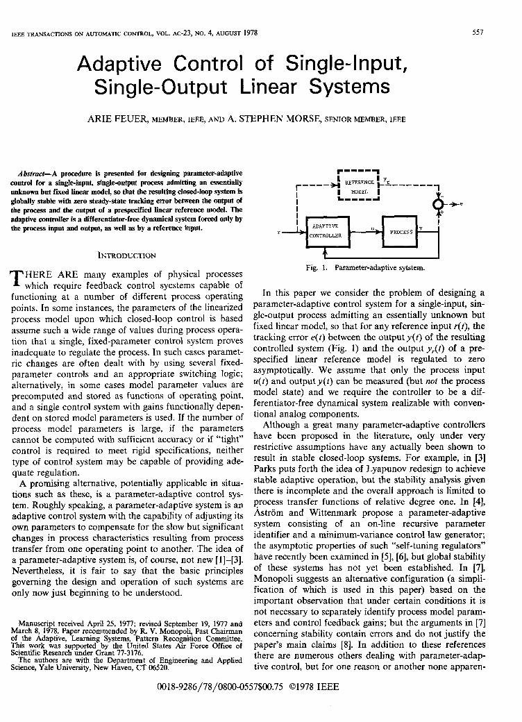
Fig. 1. Parameter-adaptive sytstem.
In this paper we consider the problem of designing a parameter-adaptive control system for a single-input, sin- gle-output process admitting an essentially unknown but fixed linear model, so that for any reference input r(t) , the tracking error e ( t ) between the output y ( t ) of the resulting controlled system (Fig. 1) and the output y,(t) of a pre- specified linear reference model is regulated to zero asymptotically. We assume that only the process input u(t ) and output y ( t ) can be measured (but not the process model state) and we require the controller to be a dif- ferentiator-free dynamical system realizable with conven- tional analog components.
Although a great many parameter-adaptive controllers have been proposed in the literature, only under very restrictive assumptions have any actually been shown to result in stable closed-loop systems. For example, in [3] Parks puts forth the idea of Lyapunov redesign to achieve stable adaptive operation, but the stability analysis given there is incomplete and the overall approach is limited to process transfer functions of relative degree one. In [4], Astrom and Wittenmark propose a parameter-adaptive system consisting of an on-line recursive parameter identifier and a minimum-variance control law generator; the asymptotic properties of such “self-tuning regulators” have recently been examined in [5], [6] , but global stability of these systems has not yet been established. In [7], Monopoli suggests an alternative configuration (a simpli- fication of which is used in this paper) based on the important observation that under certain conditions it is not necessary to separately identify process model param- eters and control feedback gains; but the arguments in [7] concerning stability contain errors and do not justify the paper’s main claims [8]. In addition to these references there are numerous others dealing with parameter-adap- tive control, but for one reason or another none apparen-
0018-9286/78/0800-0557$00.75 01978 IEEE
558 IEEE T R A N S A ~ O N S ON AUTOMATIC CONTROL, VOL. AC-23, NO. 4, AUGUST 1978
tly give an adequate answer to the following fundamental I. SYSTEM STRUCTURE question: Do parameter-adaptive controllers which yield globally stable closed-loop systems actually exist for sin- gle-input, single-output linear processes?
The purpose of this paper is to provide an affirmative answer to this question by presenting what we believe is the first parameter-adaptive control configuration, appli- cable to a reasonably large class of linear process models, which is known to result in a globally stable closed-loop system in which all signals and gains are guaranteed to remain bounded. The proposed controller requires no differentiators and can be realized with integrators, summers, gains, and multipliers. The only assumptions made about the process are that it admits a transfer function model with left-half plane zeros, and that: 1) an . upper bound for the transfer function’s “dimension,” 2) the “relative degree” of the transfer function, and 3) the sign of the transfer function’s “gain” are known.
In Section I the general structure of the controller is discussed as are the crucial process model assumptions upon which it is based; an interpretation of this structure in state-space terms reveals that the function of the con- troller is, in essence, to adaptively shift one subset of process model poles to prescribed locations, while adap- tively cancelling process transfer function zeros with the others. Detailed descriptions of the control parameter adjustment law and the auxiliary control signal needed to guarantee system stability are given in Section 11. Finally in Section I11 it is shown that application of the controller to any process satisfying the assumptions of Section I results in a globally stable closed-loop system which follows a prespecified linear reference model with zero steady-state output tracking error.
Notation
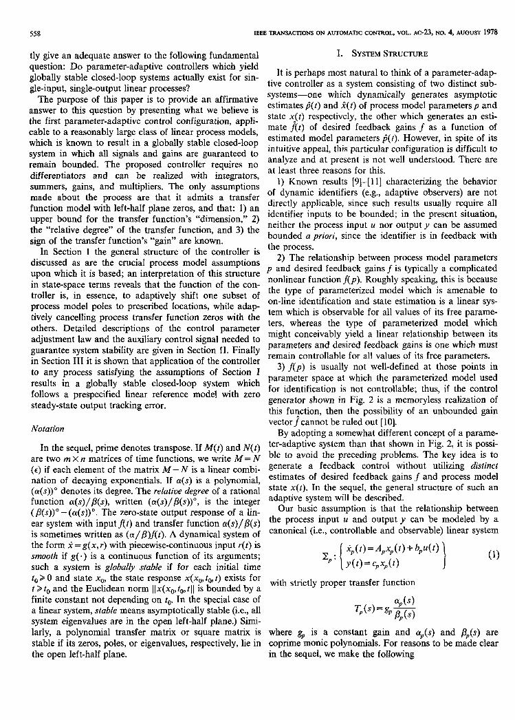
It is perhaps most natural to think of a parameter-adap- tive controller as a system consisting of two distinct sub- systems-one which dynamically generates asymptotic estimates act) and 2 ( t ) of process model parameters p and state x ( t ) respectively, the other which generates an esti- mate A t ) of desired feedback gains f as a function of estimated model parameters d(t) . However, in spite of its intuitive appeal, this particular configuration is dfficult to analyze and at present is not well understood. There are at least three reasons for this.
1) Known results [9]-[ll] characterizing the behavior of dynamic identifiers (e.g., adaptive observers) are not directly applicable, since such results usually require all identifier inputs to be bounded; in the present situation, neither the process input u nor output y can be assumed bounded a priori, since the identifier is in feedback with the process.
2) The relationship between process model parameters p and desired feedback gains f is typically a complicated nonlinear functionf(p). Roughly speaking, this is because the type of parameterized model which is amenable to on-line identification and state estimation is a linear sys- tem which is observable for all values of its free parame- ters, whereas the type of parameterized model which might conceivably yield a linear relationship between its parameters and desired feedback gains is one which must remain controllable for all values of its free parameters.
3) f(p) is usually not well-defined at those points in parameter space at which the parameterized model used for identification is not controllable; thus, if the control generator shown in Fig. 2 is a memoryless realization of this function, then the possibility of an unbounded gain vectorjcannot be ruled out [lo].
By adopting a somewhat different concept of a parame-
are two x matrices of time functions, we write M = ble to avoid the preceding problems. The key idea is to (E) if each element of the matrix M - is a linear combi- generate a feedback control without utilizing distinct nation of decaying exponentials. If a(s) is a po lyno~al , estimates of desired feedback gains f and process model
function a ( s ) / p ( s ) , written ( a ( s ) / P ( s ) ) O , is the integer adaptive system be described-
ear system with inputf(t) and transfer function a(s) /p(s ) the process input and Output y can be by a is sometimes written as (a/Plf(t). A dynamical system of canonical (i.e., controllable and observable) linear system the form f = g(x, r ) with piecewise-continuous input r(t) is smooth if g( .) is a continuous function of its arguments; such a system is global& stuble if for each initial time A t > = c,x,(t>
In the sequel, prime denotes transpose. If M ( t ) and N ( t ) ter-adaptive system than that in Fig. 2, it is POssi-
(a(s))O denotes its &gee. The relative degree of a rational state x(t)* In the the general structure Of such an
( p ( s ) ) o - (a (s) )o . m e zero-state output response of a fin- Our basic assumption is that the relationship between
ip ( t )=ApXp( t )+ b ,u( t )
to> 0 and state x,,, the state response x(x,, t , t) exists for t > t o and the Euclidean norm IIx(xo, to, tll is bounded by a with strictly proper transfer function
finite constant not depending on to. In the special case of a linear system, stable means asymptotically stable (i.e., all T , ( s ) = g , p P o system eigenvalues are in the open left-half plane.) Simi- larly, a polynomial transfer matrix or square matrix is where gp is a constant gain and $(s) and p,(s) are stable if its zeros, poles, or eigenvalues, respectively, lie in coprime monic polynomials. For reasons to be made clear the open left-half plane. in the sequel, we make the following
4 (s)
r------------------ 1 6,.(s) such that
J- I I I y(t)=gp*( b(s> u ( t ) - - u ( f ) - s y o y ( ~ ) ) 8 Y ( 3 ) (s) Y (4 ( E ) ( 4 ) d T
DY?;>MC 1 IDEX'IIII'IEII where C?u(s)/y(s) and .li,(s)/y(s) are strictly proper and
I
I ' I
I
I I L-------------------l
I I proper transfer functions, respectively. To understand the
I I role of this representation, which has its origin in [7], first
e ( t ) = y ( t ) -Y,(f) ( 5 )
GEXETUTCI + CONTROLLER observe that (4) implies that the output tracking error
Fig. 2. A parameter-adaptive system with separate identification and control. can be written as
Process Model Assumptions
1) o$(s) is a stable polynomial. 2) The following data are known:
a) The sign of g,; b) An integer n > (P,(s))O; c) The relative degree n*=(o$(s)/pp(s))O.
The principal function of the adaptive controller shown in Fig. 1 is to force the process output y to approach and track the output y, of a prespecified linear reference model. The reference model is a stable, canonical linear system
with strictly proper transfer function T,(s) and bounded, piecewise-continuous, reference input r( t). To determine what else is required of Z, for zero tracking error to be possible, let us note that if the adaptive controller shown in Fig. 1 were replaced by any linear dynamical (i.e., differentiator-free) compensator Z with reference input r, measured input y and output u, and if Tz were the resulting closed-loop transfer function from r to y , then the relative degree of T2 would not be less than n*. Indeed, this fundamental constraint on Tz can be relaxed only by incorporating differentiators in 2. Clearly, any reference model not respecting this constraint must in- volve some form of differentiation. Since we have stipu- lated that our adaptive controller be differentiator-free, we must require that (T,(s))O >n*.
The process model assumptions imply that the process can be represented in an especially useful way. To de- scribe this representation, let a(s), b ( ~ ) and y(s) be any three polynomials which have been selected with knowl- edge of n and n* so that
a) a(s ) ,p (s ) and y(s) are monic and stable. b) a ( s ) and p(s) are coprime and ( a ( s ) / / ? ( ~ ) ) ~ = n*. c) a ( s ) divides y(s) and (y(s))" > n - 1. i
(3)
where T(s)r (b(s)/a(s))T,(s); the assumptions on T,(s) (i.e., stability and (T,(s))O >n*), together with the con- straints on a(s) and p(s) dictated by (3a) and (3b) guarantee that T(s) is a stable, proper transfer function.
Next, observe that since S,(s)/y(s) and G,(s)/y(s) are strictly proper and proper transfer functions, respectively, it is possible to write
and
where the ki are constants, ny = (~(s) ) " , and {y,(s); ,y,(s)} is any preselected basis for the vector space of polynomials of degree less than nr (e.g., yi(s)= si-').' The implication of these expressions is that it is now possible to rewrite (6) as
where k [ k,, k,, . - - , k,,, + ,, 1 /g,]' is a vector of unknown constants; t9(t)r[Ol(t),02(t),. . ,02%+,(t)]' is a vector of known sensitivity functions obtained by passing u, y , and r through the stable, canonical, linear system
x,: { } (8) ~ e ( t ) = A B x e ( t ) + b , u ( t ) + b , y ( t ) + b , r ( t )
B ( t ) = Cexe ( t ) + dYy( t ) + drr(t)
with transfer matrix To=block diag { T,,T,,,T}, where
The expression for e( t ) in (7) shows that If k were known, then zero-output tracking error could be achieved
Tu=[Yl/Y,- - . ,Y,/Yl' and Ty =[YI/Y,'. - ,Y,,/YI 1Y.
It be shown in the that if p('> and Y(') IIf (?(s))">n- 1, hen Gy(s ) /y (s ) turns out to be strictly proper [cf. are SO defined, then there must exist polynomials 6Js) and Proposition 11; thus, in this case k%+, =o.
560 EEE TRANSACTIONS ON AUTOMATIC C O ~ O L , VOL. AC-23, NO. 4, AUGUST 1978
(asymptotically) by setting u(t ) = O'(t)k. Since k is not to select polynomials a, P, and y for which (4) is guaran- known, what we shall do instead is to set teed to hold, it is not only sufficient to know n* and n , but
necessary as well. Thus, even though process model u ( t ) = B ' ( t ) L ( t ) + a ( t ) (9) assumptions 2b) and 2c) may appear somewhat severe,
where i ( t ) is a suitable defined estimate of k and g( t ) is they are unavoidable consequences of any approach an auxiliary whose sole function is to guarantee based on system representation (4). Whether or not one system stability. In Section 11 we explain how to select can design an adaptive system under weaker hWotheses i ( t ) and a( 5 ) SO that for any reference input r(t) , all (e*& bY only assuming bounds for n* are known, rather system signals are bounded and e(t)+O as t - w . than n* itself) is very much an open matter.
The structure of the control law (9) is motivated prim- Remark 1: It is of Some interest to know whether Or k l y by the expression for e in (7) which, in turn, is a not a particular selection of a, P , and Y proides a consequence of (4). T~ establish the validity of (4), first ''minimal parameterization," i.e., a parameterization in note that since y(s) is a stable polynomial, y( t ) and u(t) which ap and consequently k are uniquely determined will satisfy (4) just in case y ( t ) is a solution to the by g p . $9 and P p . It can be shown that if & and Y are differential equation chosen to satisfy (14), (15), and the hypotheses of Proposi-
tion 1, then for any pair of coprime, monic polynomials o$ f i ( s ) y ( s ) ~ ( t ) = g p a ( s ) ( ( y ( s ) - G U ( s ) ) u ( t ) - 8 , ( s ) y ( t ) ) (E). and Pp satisfying (12) there exist unique polynomials 6,
and 4 satisfying (13) provided: 1) a and 5 are coprime, (lo) and 2) either y"=(P,)"- 1 or yo =(/?')" and (13b) is
Since process model assumption 1) asserts that %(s) is required to hold with inequality. While coprimeness of a stable, (1) will imply (10) if and only if and L$ can be guaranteed by simply choosing a = 1, it is
clearly not possible to choose y to satisfy 2) above, unless, -- 4 s ) 4S)(Y(S) - aU(s)) (11) of course, if (j3')" is known exactly. PPW - Y(S)P(S)+8p(s)ay(s) .
Justification of (4) thus amounts to showing that if a(s), P(s) and y(s) are polynomials satisfying (3), then there Before concluding this section we briefly outline an must exist polynomials 8Js) and 6Js) such that (1 1) holds alternative approach leading to (9), based on state-space where du(s)/y(s) and G,(s)/y(s) are strictly proper and considerations. This approach, which was what originally proper transfer functions respectively. The following pro- led us to (9), provides further insight by characterizing (9) position implies this and more. as an estimate of a desired state-feedback control law. For
simplicity, we outline the approach under the assumption that the polynomials a(s), P(s), and y(s) satisfying (3)
(y(s))" = n ; we further assume that T,(s)=g,/P(s), where g, is a constant.
The approach is based on two easily proved facts: First,
acteristic polynomial of A , then there exist n-vectors hp and bp such that
State-Space Interpretation
Proposition I : Let a,& y be fixed monic polynomials
fixed positive integers with n > n*. For each nonzero con- stant gp and each pair of monic and coprime polynomials 05 and Pp satisfving
with a and P ''Prime and ./P Proper; and let and n* be have been selected so that a(s)= 1, (P(s))O = n* and
( $ l P p ) " = n* (12a) if ( c l x n , A n x n ) is any observable pair, with y(s) the char- and
(P,)" Qn (12b) o$ (4
there exist polynomials 8, and 8, satisfving c(s l -A-h,c)- 'b ,= - B p ( 4 * (16)
(44/Y)O>O (13a) Second, for at least one pair (hp,bp) satisfying (16), there @,/Y)" 2 0 (13b) exists a row vector f, such that A + hpc + bpgJp is stable
and (1 l), i f and oniy if a divides y, and
(14) ( a / P ) " = n * , c (sI -A-h,c-bpgJp)- 'bp=- . P(s ) (17) 1
and Equation (1 6) implies that (y)" > n - 1 (15)
i p ( t ) = ( A +h&,(t)+b,g,u(t) If a, f i and y have the required properties and if the y ( t )=cxp( t )
inequality in (15) is strict, then there exist 8, and 6, satisfv- ing (11) and (13) for which the inequality in (136) is strict. is a process model. sine ip cafl also be written as
A proof of this proposition appears in the Appendix. The proposition clearly implies that in order to be able i p ( t ) = ( A + hpC+ bpg&)Xp ( t ) bpgp ( u ( t ) - f , X p ( t > )
FEUER AND MORSE: ADAF’TNE CONTROL OF LINEAR 561
and since A + h,c + bpgJp is stable, we can use (17) to obtain
By assumption, y,(t) =(g,/P(s))r(t), so the output track- ing error can now be written as
e(t> = B P - ( U ( t ) -f,x,(t) - (g,/gp)r(t)) ( 4 (19) P(s )
This suggests that desired system behavior might be achieved by setting u(t)=f(t)f(t)+g(t)r(t) wheref(t),I(t) and g ( t ) are suitably defined estimates of f,, x,(t) and g,/g,, respectively-but as mentioned at the beginning of this section, this approach leads to difficult problems which so far have not been overcome.
The alternative approach pursued here is to use an estimate of the product f , x , ( t ) rather than the product of estimates off, and x,(t), respectively. The structure of the proposed estimate is motivated by the fact that the state xp( t ) of system (1 8) can be written as
.,(t)= Eu(t)bpgp + Ey(t)h, + eA‘q (20)
where E,([) and E,(t) are any pair of solutions to the matrix differential equations
& ( t ) = A E , ( t ) + l u ( t ) ky ( t )=AEy( t )+Zy( t ) (21)
root set of %(s)P(s). The more general situation, when a, /I, y, and T,(s) are not constrained by these special assumptions, admits a similar state-space interpretation, provided system (18) is replaced with a more general linear model, representing the process together with a dynamic compensator.
11. CONTROL EQUATIONS
To complete our description of the proposed adaptive system, we first select a($) and P(s) so that (3) holds, and in addition so that P(s)= P*(s)S(s), where P*(s) is monic and a(s)/P*(s) is a strictly proper, strictly positive real transfer function. It is easy to check that these constraints imply that S(s) must be a monic, stable polynomial of degree n* - 1.
It turns out in what follows that nothing essential is lost if a(s) /P* (s ) is assumed to be the transfer function of a one-dimensional system, i.e., a ( s ) / P * ( s ) = l/(s +xo> for some b>O. For the sake of simplicity we henceforth make this assumption; the more general situation in which a(s)/P*(s) is the positive real transfer function of a higher dimensional system can be treated along similar lines using the Kalman-Yakubovich lemma.
These assumptions together with (5) and the control law defined by (9) imply that the output tracking error e(t) can be written as
I is the n X n identity and q is a constant vector depending where is the parameter error on the initial values of x,, E,, and E, [lo]. Since A is a stable matrix by hypotheiis, it followifrom (20) that Z ( t ) = J c ( t ) - k .
f,xp(t)=f,E,(t)b,gp+f,E,(t)h, (€1- (22) We wish to develop a parameter adjustment law for k(t) and an expression for a(t). Since these equations are
for the case n* = 1, these cases will be treated separately. Using just (21), (22), and the Of A , it is not considerably more compficated for the n* > 1 than difficult to verify that f ,x,(t) can also be written as
will yield an estimate off,x,(t)+(g,/g,)r(t) provided &(t) is an estimate of ki for iE{1,2,...,2n} and k(2n+I)( t ) is an estimate of l/g,.
The preceding development shows, at least under the special assumptions on a, P, y, and T,(s), that the term eyt)L(t) appearing in (9) is really an estimate off,x,(r)+ (g,/g,)r(t) where f ,x,(t) is a state feedback law, whch if applied to process model (18), would have the effect of shifting the model’s poles from the root set of P,(s) to the
Z,-: i ( t )= -(sign(g,))@(t)e(t), (26)
where Q is any prespecified, positive definite, constant gain matrix, then for any reference input r(t), bounded for t > 0, and for any initial time to > 0 and state xz(to), the state response xx( t ) = (x,( t) , x,( t) , xs(t), k( t ) ) of the result- ing closed-loop adaptive system Z described by (I), (2), (5), (8), (9), and (26) exists for t >to and is bounded uniformly in to. To understand why this is so, first observe that we can now use (24)-(26) to write
562 IEEE TRANSACTIONS ON AUTOMATIC CONTROL, VOL. AC-23, NO. 4, AUGUST 1978
E( t )= -(sign(gP))Q8(t)e(t) (2%)
where e ( t ) is a linear combination of strictly decaying exponentials. Next observe that since Z is smooth dy- namical system, for any initial time to > 0 and any initial state x;, there must be a nonempty interval [to, T ) of maximal length on which xz( t ) exists. If the derivative of the nonnegative time function
is evaluated on [to, T ) there results from (27)
(29) Since pQ 0 and V > 0, it must be that 0 Q V(t) < V(to); this and (28) clearly show that e( t ) and E(?) are bounded on [to, T ) by a constant not depending on to or T. Bounded- ness of E(t) and (25) imply boundedness of &t), whereas boundedness of r( t ) for t > 0 and stability of Z, imply boundedness of x,(t); the latter together with bounded- ness of e( t ) and ( 5 ) imply boundedness of y(t). To prove that x,(t) is bounded, it is therefore enough to establish boundedness of u(t ) ; in view of (9) and the hypothesis E ( t ) = 0, u(t) will be bounded provided O(t) is. Since both r ( t ) and y ( t ) are bounded and since (8) is a stable system, it follows that 8( t ) [and xe(t)] will be bounded provided (sZ - A,)-’b,u(t) is; but (sZ - A,)-’b,u(t) = ((sZ - A,)-’b,(s+ l))(l/(s+ l ) )u ( t ) ( E ) and sl-A,)-’b,(s+ 1) is a proper transfer matrix. To establish boundedness of (sZ- A,)-’b,u(t) it is therefore enough to show that (l/(s + l ) )u ( t ) is bounded. To do this we make explicit use of process model assumption 1) and the hypothesis n* = 1 to conclude that (1 /(s + I))( G(S))-’ is a stable, proper trans- fer function. Since (1 /(s + l))u(t) = (1 /(s + I))( T,(s))- 5(t) (E), and since y ( t ) is bounded, it follows that (I/(s + I))u(t) is bounded as well.
The preceding argument shows that xz( t ) exists and is bounded on [to, T ) by a constant not depending on to or T. The latter property together with the smoothness of Z ensure that xz(t) can be extended to [ T, cc) so that for all t E [ to, m), xz( t ) satisfies Z’s state equation and is bounded uniformly in t,.
To show that e(t)+O as t+m we first use (28) and (29) to conclude that V(t) is a monotone nonincreasing func- tion of t ; since, in addition, V(t) > 0, it must be that V,,=lim,,,V(t) < co. This shows that the integral lCV(7)dr converges. Since, in addition, (29) and (27) imply that both v(t) and p(r) are bounded on [to, co), it follows that lim,+, f ( t ) = O , and hence with (29) that e(t)-+O as t+m. The following theorem summarizes what has been established thus far.
Theorem I : If n* = 1, if r ( t ) is any reference input,
bounded and piecewise-continuous on [0, co), and if Z is the closed-loop adaptiue system described by (l), (2), (5), (S), (9), (26), and E ( r ) = 0, then for arbitraly initial time to > 0 and initial state x; and for all t >to, the state response x,(t , to,.;) of Z exists and is uniform& bounded in t,. In addition, along any such state response, the system’s output tracking error satisfies
lim e( t ) = 0. r + c o
General Case n* > 1
For the remainder of this paper we focus attention on the more general and considerably more difficult case when n* > 1. Since 6(s) is now necessarily of positive degree, implying that the transfer function 1 /((s + h)6(s)) in (24) is no longer positive real, to proceed it becomes necessary to introduce auxiliary filters of much the same structure as those first proposed by Monopoli [7]. These filters are described by the equations
E i ( t ) = A H ( t ) + bO’(t) (304 +‘( t ) = cH( t ) (30b)
and
where (c , A , b) is an (n* - 1)-dimensional realization of l/S(s), H ( t ) is an (n* - 1) X (2n, + 2) matrix, and x(t) is an (n* - 1)-vector; specific equations for k^(r) will be given in a moment.
Using (24), (30), (31), and the assumed stability of A , it is straightforward to verify that
Thus, if F ( t ) is an auxilialy error defined by the equations
2%: [ i o ( t ) = -X,+o(t)+g(t)cx(t) (324 a( t )=x , ( t )+e( t ) (32b)
where g( t ) is a signal intended to estimate g,, then it is possible to write
i ( t ) = - & ~ ( t ) + g , + ’ ( t ) E ( t ) + c x ( t ) g ( t ) + E ( t ) (33)
where
a t ) = 2 (1) - g,. (34)
and c ( t ) is a linear combination of strictly decaying ex- ponential time functions. The significance of (33) is that it has much the same structure as (27a). This suggests that system stability might be achieved by setting ir( t ) = 0,
%: i ( t ) = -(sign(g,))Q+(t)P(t) (35)
and
FEUER AND MORSE: ADAPTIVE COhlROL OF LINEAR SYSTEMS 563
where Q is any preselected positive definite, constant, gain M , = ( C , P - ' C ; ) - ' matrix, and q is an arbitrary positive constant. Indeed, for any choice of ii(t), (35) and (36) imply that
i - 1 M ; = ( c j P - ' c ; ) - l I i x i - x C i P - q l y E J , ,
j = 1
L ( t ) = - ( s i g n ( g p ) ) Q 9 ( t ) c ( t ) (37) 1 &t)= - qcx( t ) e ( t ) (38)
and thus with (33) that the time derivative of the nonnega- tive function
( e ( t ) - t l g p l k " ( t ) Q - ' E ( t ) + - g 2 ( l ) 1
2 4 V(t )= L -2
For the same reasons as before, it can be concluded from (39) and (40) that F(t), &to, and g( t ) are bounded time functions on some interval [ to ,T) of finite length; how- ever, from these two equations and (32) it is not possible to conclude that e(t) is bounded since there is no guarantee that cx(t) is. Indeed one can construct an example with ti(t)= 0, for which cx( t ) is not bounded assuming x ( t ) is a solution to (31) [SI. However, since this example uses a contrived H ( t ) rather than one known to satisfy (30a), the example does not really demonstrate system instability. On the other hand, the example does show that much more elaborate arguments involving the equations which generate both H(t ) and O(t) are required to prove boundedness, at least for the case E(t)=O. Although we have recently obtained results suggesting that the adaptive system obtained by setting G(t)=O [with &(t) and g( t ) as defined in (35) and (36)] actually has a bounded state response for any bounded reference input [ 121, this issue is not yet settled.
To achieve a bounded state response, we shall continue to use the parameter adjustment laws for &t) and g ( t ) as given by (35) and (36), but we shall no longer take ~ ( t ) to be zero. Instead we shall set
where f ( H ) elements of
U = f ( H ) x (41)
is a row-vector of polynomial functions of the H ; f(-) and is defined as follows. With
#En* - 1 and Po any preselected A X ff positive definite matrix, write P for the unique positive definite solution to the equation
i ~ { 2 , - * . , A } (48)
- ( C A i - ~ + g ; - , c ; - , ) N , , i E { 2 , . . * ,a} (49)
where I
N i = P - ' 2 q M . J w.w!M.'E. J J J J , l . (50) j - 1
and
Ri+ 1 = [O"ix i ] ;x( i+ 1); (5 1)
hij is the j th column of CiH and agi-, /ahi- ,,; is the ( i - 1) X j matrix of partial derivatives of g i - ' ( C i - I H ) with respect to the elements of hi- ld . It is important to note that these definitions imply that g,, w,, and hence Nj are matrices of polynomial functions of the elements of CiH.
Next observe that because of the structure of matrices Ejj defined by (45), the A X A matrix
0 g,J%n
g2E2, iz G= I +
- gii- 1%- 1,n
PA + A'P= - Po. is lower triangular, with ones on its diagonal. From this (42) and the aforementioned function dependence of gi on
For k { 1,. , E } , let Mi denote the i x i matrix CiH, it follows that G - ' exists and that the elements of
564 TRANSACTIONS ON AUTOMATIC CONTROL, VOL. AC-23, NO. 4, AUGUST 1978
both G and G are polynomial functions of the elements of H . Hence, iff is now defined as
then f is a row-vector of polynomials in the elements of H.2 Our specific reason for defining f in this way will become apparent in the next section.
To summarize, the proposed adaptive controller for the case n* > 1 consists of the reference system Z, defined by (2), the output tracking error (5), the sensitivity function system Z, defined by (8), the control law (9), the filtered sensitivity function system E,, defined by (30), the aux- iliary error system Zx0 defined by (32), the parameter adjustment laws (35) and (36), and the system
Z , : i = ( A -b f (H) )x -HQH'c 'F(s ign(g , ) ) (54)
which results when the expressions for i, 9, and ii given by (35), (30b), and (41) respectively, are substituted into (31). Careful examination of the equations involved re- veals that the resulting adaptive control system consisting of Zr, Zp, Z,, Z,, Z,, Z,, EL, and Z, is a well-posed dynamical system in that within each feedback loop, there is a strictly proper transfer function.
111. SYSTEM STABILITY
Our main result is as follows.
Theorem 2: If n* > 1, i f r( t ) is any reference input, bounded, and piecewise continuous on [0, X I ) , and if Z is the closed-loop adaptive system described by (I), (2), (51, (8), (9), (30/, (32), (35), (36), and (54), then for arbitrary initial time to > 0 and initial state x: and for all t > to, the state response xz(t, to,xg) of Z exists and is bounded uniform& in t,. In addition, along any such state response,
lim e(t)+O
lim x(t)+O
I - t o C
r-tm
lim xo( t)+O. I+W
The adaptive system Z can be viewed as a dynamical system of the form 2z=p(xz , r ) , where x x is a composite state vector consisting of subvectors k, e, xp, x,, X,, H , x , and xo, and p is a continuous function of xz and r . Theorem 2 clearly implies for any fixed, bounded r(t) , that the zero solution to the differential equation $= p(i?,r(t))- p(Xo(t),r(t)) is globally, uniformly stable, jSo(t) being the (bounded) state response of Z to r ( t ) assuming a zero initial state at time to = 0. It is in this sense that Z can be characterized as a Lyapunov stable adaptive system.
In view of the preceding theorem and the structure of R as defined by (41), it is clear that is(t)+O as t+co. On the other hand, it cannot be concluded from Theorem 2 (or Theorem 1) that the parameter errors F(t) and g(t) tend to
'Note that C; is nonsingular because (c,A) is observable.
zero as t+m. In fact, these errors can be expected to go to zero only if the process model on which controller design is based is minimally parameterized (see Remark 1). If this is the case and if r ( t ) is in some sense "per- sistently exciting," then it is at least plausible that both &t) and g( t ) will asymptotically approach zero. It appears likely that this can be shown to be so without too much difficulty using (for example) the results of [ 1 1 1 .
The proof of Theorem 2 depends on six lemmas. The first describes certain algebraic relationships which exist between a positive-definite matrix P and matrices Mi defined by (43).
Lemma 1:
R
P = 2 c,IMjcj J= 1
(55)
and
Prooj The definition of Mi in (43) implies that
If both sides of this equation are postmultiplied by Ci and if C, is then substituted for Ek,;Ci, there results
Equation (55) is obtained by premultiplying each side of (57), at i = R , by P(CB)-' .
To establish (56), replace i with j in (57) so that
If, for j > i , both sides of this equation are premultiplied by Eij and if Ci is then substituted for E&, there results
Subtraction from (57) thus yields
from which (56) follows. 0 The next lemma is a simple consequence of (30) and of
the definition of (c ,A,b) .
Lemma 2:
+'= C , H (584
CiH=Rj+ lCj+ lH i E { 1 , 2 , . . - , ~ - 1 } (58b) c ~ f i - l H = c ~ f i ~ + ~ ' (584
Pro08 Equation (58a) is a direct consequence of
(30b) and (44). Since (c ,A,b) canonically realizes 1/6(s), of '2:i. Thus CA'-'Sw equals g;-1'Vi-1 PIUS the ith row of it must be true that CA A- lb = 1 and that c~ i-1b =o, i E wj . From this and the definition of w, in (48) it follows that { 1; . . ,A- I > . The former and (30a) imply (58c), whereas (69) is true for this value of i. the latter clearly show that C;.b=O, i E { l , - . * , E - l } . The preceding argument proves that (69) holds for Hence using (30~1, c,a = CJH, i E { 1,. . . , E - 1 ) ; from i E { 1, . . , A } . Since ( c , A ) is an observable pair, we have these expressions and the identity R,+ , Cj+ , = C,A, it h w n that (64) is true. follows that (58b) is true. 0 Next consider the expression
The following lemma describes the key algebraic rela- I
tionships upon which our stability proof is based. N , c ; = P - I x qMjc,wiv'c,",'c,, iE{1,2;-,E} ;= 1
Lemma 3: I f S E (CJ- 'GC, and
z = s - ' x
then
which is what results if both sides of (50) are postmulti- plied by Cj and if cj and CJw are then substituted for
(59) E,.,C,, and y, respectively. In view of (56) and the defini- tion of X in (66), it follows that
...=(C,)-'\l?,-. (62) To develop similar expressions for cA 'S, i > 1, we first
Proof: In view of (54) it is enough to show that use the identity [ g , _ , , l ] C j = c A ' - ' + g , _ , C i - , , i E { 2 ; . * , E}, together with (68) and (70) to obtain
cs= c
Sw = - HQH'c'(sign (g , ) ) (64) (63) ( c A ' - ' + g , _ , ~ , - , ) ~ 7 ~ ~ , = c ~ i - ~ ~ ~ , i E { 2 ; * - , A ) .
(72) and Next we exploit the fact that for i E ( 2 , - . . ,E>, g,- , de-
S + S ( A - X ) = ( A - b f ) S (65) pends only on Cj -, H . This enables us to write
where
x= P - I x c;M~c,ww'C,";c~. (66) i = I where hi- ,., is the j th column of C , - , H . Using (58b)
which impkes that h ' i - l , j = RjhjJ, i E ( 2 , . ,E}, we can From (45) and (48), wj = Ej,nwn, i E {I , 2, * - ,E}; hence write
by (62), w, = Ej,nCnw. Since (44) and (45) provide the identities C;. = Ei,nCA, i E { 1,2,. . . ,E>, we can write * ( f l y + 1) 2 h,!,R,'- i E (2; , E } . ag; - 1
w ; = c ; w , iE{1,2;-,E}. (67) ;= 1 ah,- '
The definition of G in (52) implies that c is the first row of GC, and, for i> 1, that cA'-'+g,E,,,C, is the ith row. Since GC,= CAS, the ith row of CAS, namely cA'-'S, must satisfy (63) for i = 1 and cA '-IS = cA ' - I + gi- lEi- l ,RCn for i > 1; using the identity C j P l = Ei-l,ACn, i E (2, . ,E>, the latter can be written as
c~i - l s=c~i - l +g,-,c,-,, i E { 2 , - * * , ~ } . (68)
Since c = C,, (63) and (67) imply that cSw= wI; from this and (46) it follows that the equation
cA '-'SW = - CA '-'HQH'c'(sign (g , ) ) (69)
holds for i = 1. Now fix i E (2 , . . ,A> and use (67) and (68) to obtain c A ' - ' S ~ = c A ' - ' w + g , ~ ~ w , ~ ~ . Note that cA '-Iw is the ith row of C,w which by (67) is the ith row
Since E;- , , /Cj = C,- it follows that
If for i E (2; . ,E} the expression defining g, in (49) is postmultiplied by Cj and if (72) and (73) are then sub- stituted into the result, one obtains the expression
g j C j = g j _ l C j ~ , + g , _ , R , C j - c A ' - l S X , i E { 2 ; - . , A ) .
Addition of CA ' to both sides, followed by substitutions of C j - , A for R,C,, cA'-'S for cA'- '+g; . - ,C , - , , and cA'-'S for g, - ,Cj- , yields
566 IEEE TRANSACTIONS ON AUTOMATIC CONTROL, VOL. AC-23, NO. 4, AUGUST 1978
For iE{2,... , R - l}, (68) implies that the left side of (74) can be replaced by CA 'S. This together with (71) allows us to write
CA'S=CA' - ' (S+S(A-X) ) , i € { l ; * - , E - ~ ) .
As noted in the proof of Lemma 2, CA '- 'b = 0, i E { I , - . - , R - 1 } ; thus the preceding expression can be writ- ten as cA i - I ( A - b f ) S = c A ' - ' ( $ + S ( A -X)),
i E { 1;. . ,E- 1). (75)
The definition off in (53) implies that fS+ CA "+g,C, = CA "S. Since CA "b = 1, we can write CA "- ' (A - bf)S = cA"+ g,C,. From this and (74), it is now clear that (75) also holds for i= E. Since ( c , A ) is observable, it follows from (75) that (65) is true.
C,i= C,Az+ C,WE- CiNic . z , i E { 1,- - . ,R- I}.
To obtain the desired result, substitute &.+ Ci+ for C,A, Ei , i+lCi+, for C,, and use (67) to replace C,w by wi.
Lemma 5: It is possible to write
e(')=E4.(P,~g,x,C,H,Ciz,Ei), i € { l ; . - , A > (76)
where e('? is the ith derivative of e, E, is a linear combination of decqving exponential time functions, and p j is a continu- ous function of its arguments.
Proof: Observe from (32b) that e = P - x,. If this ex- pression is differentiated, if (32a) and (33) are used to eliminate derivatives, and if (34), (58a), and (60) are then used to eliminate 2, +, and cx, the resulting expression is ~ = p l ( P , ~ , g , ~ o , C I H , C 1 ~ , ~ l ) where p1 is an infinitely dif- ferentiable function. If this expression is, in turn, differen- tiated, and if (32)-(34), (37), (38), Lemma 2, and Lemma 4 are used to express e in terms of E,,,g,x,, C2H, C2z,c2, w , ( C , H ) , and N , ( C , H ) , then there results e = ~ ( E , ~ , , g , x , , C,H, C2z,e2) where 1fl2 is an infinitely differen- tiable function of its arguments. Repeating this process and making use of the fact that wj and Nj depend only on C,H, one obtains a sequence of infinitely differentiable (and hence continuous) functions for which (76) is true.
0 Lemma 6: There exist proper, stable transfer matrices
T(s), T,(s) , . * , T,(s) such that
cA'H=(T(s)e( ' )+T, (s )r ) ' (E), ~ E { O ; . . , A - I }
(774 and
P=( T(s)e(')+ ~ , ( s ) r ) -CA 'IH (e ) . (7%)
Proof: Definitions (8) and (30) of 8 and H , respec- tively, imply that
1 TUU x] (78)
where 1/6, Tu, Ty, and T are stable, proper transfer matrices. Since Tu is actually strictly proper and since (l /S)"=(T,)"-I, it follows that (l/8)(T,)-'Tu is a proper transfer matrix; by process model assumption l), (1 /a)( T,)- 'Tu is also stable. In addition, since y = Tpu we can write (l /S)T,u=(l/S)(T,)- 'T~ ( E ) . Substitution in (78) then yields
where Tr(l/&)[( T,)-lT;, T,',O]' is a stable, proper trans- fer matrix. From (2) and (5), y = e + T,r; substitution in (79) thus provides
where To TT, + [0, 0, (1 / 6) TI'. Since, by assumption, T, is a stable transfer matrix satisfying (T,)" 2 (T,)", and since A = (T,)" - 1, it follows that To is a matrix of proper, stable transfer functions, each of relative degree no smaller than A. Thus if q ( s ) is now defined to be s'T,(s), i E { 1,. - - , iT}, then T, must be stable and proper and by (80), the ith derivative of cH, written cH", must satisfy
But Lemma 2 implies that cH(')= cA'H, i E (0;. ,E- 1 ) and that C H ( ~ = 8 ' + CA 'H. From these relations (80) and (81) it now follows that the lemma is true. 0
Proof of Theorem 2: Let r(t) , to> 0 and x; be fixed. The smoothness of Z implies that for some T >to, the state response xz( t ) exists on [to, T). With E(t) as in (33), let V(t ) denote the nonnegative time function
+ kJffie2(?)d7 + Y z ' P z . (82) 1 : Differentiation of V, elimination of resulting derivatives using (33), (37), (38), (61), completion of the square in e and E, and substitution of Po for - (PA + A ' P ) yields
Using (55) to eliminate P from the preceding expression,
followed by completion of squares, provides
Equations (82) and (83) clearly imply that V, E, E, 8, and z are bounded on [to, T ) by a constant not depending on to or T. It will now be shown in six steps that the eight constituents k, $, x,, H, x , x,, xp, X, of the state response of I: are each bounded on [to, T) .
1) Boundedness of k̂ and 2 are direct consequences of (251and (34), respectively , together with the boundedness of k and g, respectively.
2) Boundedness of x,-Boundedness of z and (60) im- ply that cx is bounded; from this (32a) and the bounded- ness of it follows that x, is bounded.
3) Boundedness of H-Boundedness of .? and x,,
of F, z, and H clearly imply the former, it is enough to establish the latter. Differentiation of the expression in (83) shows that is a continuous function of the quanti- ties P, E, w, z , ;, <, w , and i. Boundedness of ; follows from (33) together with the boundedness of e, E, x, E, E, and +’(= cH). Boundedness of i is obvious, since E is a linear combination of decaying exponentials. Recall that wE is a polynomial function of the components of H ; since w = C,w,, this and boundedness of H and H (which is a consequence of (30a) and boundedness of 6) imply boundedness of G. Boundedness of i follows from (61) and the boundedness of t, w, and Z. Thus v(t) is bounded for I > 1,.
The preceding argument proves that V(f)+O as t+m. Examination of (83) reveals that this can occur only if and z approach zero as t+m. Since from (59) x = Sz and since S depends continuously on H , it follows that S is bounded and thus that x( t)+O as t+m. This together with (32a) and the boundedness of $ imply that x,(t)+O as t-00. It now follows from (32b) that e(t)+O as t+m.
n together with (32b) imply boundedness of e; since r is also bounded, it follows from (77a) that cH (i.e., C , H ) is bounded. If for fixed i <A, e(’-’) and CiH are bounded, then by Lemma 5 e(i) is bounded, and thus by Lemma 6 CA ‘H and hence Ci+ ,H are also bounded. By induction, C,H and thus H are bounded.
4) Boundedness of x-By Lemma 3, x= Sz. Since S depends continuously on H and since both H and z are bounded, it follows that x is bounded.
5 ) Boundedness of x, and x,-Boundedness of Y and stability of X, clearly imply boundedness of x,. This together with (5 ) and boundedness of e imply bounded- ness of y . Since X, is a canonical system with a bounded output, to establish boundedness of xp it is enough to show that u is bounded. For this, first observe that boundedness of H together with Lemma 5 imply boundedness of e(@; thus by (77b), 0 is bounded. Next observe that (9) and (41) imply that u depends continu- ously on k, e , ~ , x, and f; since 6, e, and x are bounded and since f depends continuously on H, which is also bounded, it follows that u and therefore xp are bounded as well.
6) Boundedness of is a consequence of the stability of Z, and the boundedness of u, y , and r.
The preceding arguments prove that x,(t) is bounded on [to, T ) by a constant not depending on to or T. From this and the smoothness of 2 it follows that x=([) can be extended to [T, 00) so that for all t > to , xz(t) satisfies 1’s state equations and is bounded uniformly in I,.
To prove that e, x , and x, approach zero as f+m, it will first be shown that Fi(t)+O as t+m. For this, observe from (83) that p< 0; thus V(t ) is a monotone nonincreas- ing function of t, bounded below by zero. This implies that l i n~ , -~ v(t)< 00 and thus that the integral Jc p(t)dt converges. Therefore v(t) will approach zero provided p(t) and v(t) are both bounded for t >to; since (83) together with the continuous dependence of w on H [i.e., w = C,w,(C,H)] and the already established boundedness
U
CONCLUDING REMARKS
In this paper we have outlined a procedure for design- ing a parameter-adaptive controller capable of causing the output of a process to approach and track the output of a prespecified reference model with zero steady-state error. While the controller is admittedly complex, to our knowl- edge it is the only differentiator-free dynamical adaptive controller proposed thus far which, without making un- necessarily restrictive process model assumptions, has been shown to provide globally stable closed-loop opera- tion when applied to a single-input, single-output linear system. Whether or not global stability can also be achieved with other, possibly less complex adaptive con- trollers (e.g., the one considered in this paper with U=O) is an interesting question for further study.
The principal result of this paper-that it is actually possible to adaptively control a linear system with zero steady-state tracking error-is contrary to our earlier ex- pectations [lo]. The reservations expressed in [ 101 are prompted by the observation that with certain adaptive configurations, unbounded controller gains might result as current estimates of process transfer function coefficients approach values for which the estimating transfer function has a pole and zero in common. What this paper shows is that this problem can be avoided by applying to the process a control signal which, in effect, is an estimate of the product of desired feedback gains and process state rather than the product of distinct estimates of desired feedback gains and process state. At present, the genera- tion of such a control signal seems possible only for those desired feedback laws which, if applied to the process, would cause all process transfer function zeros to be cancelled. For this reason, it is not clear if the possibility of unbounded gains can be avoided in those situations where “adaptive-zero cancelling” cannot be employed
568 IEEE TRANSACTIONS ON AUTOMATIC CONTROL, VOL. AC-23, NO. 4, AUGUST 1978
(i.e., when the process transfer function has right-half plane zeros.)
Since Theorems 1 and 2 are true, independent of the stability of the open-loop process model, the results pre- sented here are potentially applicable to the problem of identifying process models not assumed to be open-loop stable. Recent simulation experiments have shown, that for such models, the overall set of differential equations describing the adaptive system can be quite sensitive to computer roundoff errors unless the initial parameter errors are small. Such problems, which we believe to be characteristic of all parameter-adaptive algorithms, can apparently be minimized by appropriately choosing the various gains associated with the adaptive algorithm. Sys- tematic techniques for selecting these gains to reduce sensitivity or to increase convergence rates are obviously needed, but so far have not been developed.
APPENDIX
Proof of Proposition 1
Sufficiency: Suppose that a, p, and y satisfy (14) and (15) with a dividing y. Write o and p for the unique quotient and remainder of by divided by a@,; thus
PY=aPpo+P (All
where po <(a&,)". Since by hypothesis, a divides y, it follows from (Al) that a divides p; thus p= ap where j j 0 <( p,)". If 8, is now defined so that 6, = -(l/g,)p, then
PY = - g,6,. ( a and (6,)" < ( p,)". The latter together with (12b) and (15) ensure that 8, satisfies (13b); and if (15) is a strict inequal- ity, then so is (13b).
Since po <((up,)", (Al) implies (a/?,o)" =(py)"; thus (ap,u%)" = (pyq)". In addition, since (12a) and (14) im- ply (pq)" =(&x)", it follows that (ap,u%)" =(yp,a)"; hence, (ug)" = yo. Since (Al) also implies that o is monic and thus that ug is monic, if 8, is defined as
8u=y-acup ( f w
then (13a) must be true. Elimination of o from (A2) and (A3) now yields (1 1) which is the desired result.
Necessity: Let 4 and pp be polynomials satisfying the proposition's hypotheses with 4 and a coprime and (P,)" = n ; such polynomials clearly exist. Suppose that 8, and 8, are polynomials satisfying (1 1) and (13). Since a and 4 are coprime, it follows from (1 1) that a divides y p ; but a and p are coprime by hypothesis, so a must divide y as the Proposition asserts.
Since q and aP, are coprime, (1 1) will hold provided
up=y-6, 644)
o.P, = Y P + g@y (A51
and
For some polynomial o. From (A4) and (13a) it follows that
y"=(oq)".
By hypothesis, both a /P and 8,/y are proper; hence (UP)" > (UP +gpa8y)o- This and (A51 imply (YP)" > (aap,)"; but from the relation (oap,)" =(uap,cup)" - (%)" and (A6) there follows (oap,)" > (yap,)" -(%)". Thus ( yp ) " > (yap,)" -(g)". This and (12a) imply that 8" >a" + n * ; but n* >0, so po>ao. From this, (M), and (13b), it now follows that
Substitution of (A6) in (A7) and elimination of common factors yields (a@" = (gB)"; from this and (12a), it now follows that (14) is true.
Since (15) must necessarily hold for n = 1, assume n > 2 and suppose (15) is false. Then yo < n - 2; since ( p,)" = n,
(@,)"-y0>2. (A8)
From(12a) and (14), / 3 " = ( ~ , ) " + a o - ( ~ ) 0 . Since (A6) implies (4)" < yo, it follows that
p" > ( p p ) o +ao -yo*
Choose p so that
p o = a o + l (AW
and so that p - p has a root as s = 0. Since (A8) and (As) imply p" >a"+2, it follows from (A10) that p " > p " ; hence ( p - p ) " = P o . Therefore, from (A9) ( p - p ) O > (P,)" + a" - y o . Since ( P - p ) has a real root, it follows that there is a factorization
p - p = a (A1 1)
e o = ( p p ) o + a o - y o . ( A m
where 8 is a monic factor satisfying
From this and (A8), there follows 8" >a" +2. Therefore from (A10) 8">p". This and (All) can be true only if p is the unique remainder of least degree of p divided by 8.
Since a divides y, there must be a polynomial & such that a& = ye. Since (A12) implies that (6)" =( p,)" and since PP is defined independent of p,, we can assume that pp was selected at the outset so that pp =$. Thus (upp= y8. Hence from (A5), oy8 = y p + gPa6,. Thus we may write
p=eu+c (A131
where 5 is a polynomial satisfying
c y = - gpaGy.
Since p was shown to be the unique remainder of least degree of /3 divided by 8, it follows from (A13) that
FEIIER AND MORSE: ADAPTIVE CONTROL OF LINEAR SYSTEMS 569
f i o , j j o . This and (A14) imply that a”+(S,)” >y”+po. Hence from (A10) ao+(S,,)O>yo-!-ao+l; thus (Sy)o>yo + 1 which contradicts (13b). Hence (15) is true. 0
[41
[51
181
[91
REFERENCES
R. E. K h a n , “Design of a self optimizing control system,” Trans. ASME, vol. 80, pp. 468-478, Jan. 1958:
York: McGraw-HiU, 1967. W. Everleigh, Aabprioe Control and Optmiration Techniques. New
P. C. Parks, “Liapunov redesign of model reference adaptive control systems,” ZEEE Trans. Automat. Contr., vol. AC-11, pp.
Automatica, vol. 9, pp. 185-199, 1973. K. J. Astrom and B. Wittenmark, “On self-tuning regulators,”
L. Ljung and B. W~ttenmark, “On a stabilizing property of adap tive regulators,” Preprints, ZFAC Symp. on Identification and *st. Parameter Estimation, Tbilisi, USSR, 1976. L. Ljung, “On positive real transfer funchons and the convergence of some recursive schemes,” IEEE Trans. Automat. Contr., VO~.
R. V. Monopoli, “Model reference adaptive control with an aug- mented error signal,” ZEEE Trans. Automar. Conrr., vol. AC-19,
A. Feuer, B. R. Barmish, and k S. Morse, “An unstable dynami- cal system associated with model reference adaptive control,” IEEE Trans. Auioma:. Conrr., vol. AC-23, pp. 499-500, June 1978. G. Liiders and K. S . Narendra, “An adaptive observer and identi- fier for linear systems,” IEEE Trans. Automat. Contr., vol. AC-18, pp. 496-499, Oct. 1973.
multi-output linear systems,” in Proc. IEEE Conj: on Decision and A. S. Morse, “Representation and parameter identification of
A. P. Morgan and K. S . Narendra, “On the stability of nonautono- Contr., 1974, pp. 301-306.
matrix B(t),” SZAM J. Contr., vol. 15, pp. 163-176, Jan. 1977. mous differential equations i = [ A + E(r)]x with skew symmetric
A. Feuer and A. S . Morse, “Local stability of parameter-adaptive control systems,” in Proc. I978 Conj: on Znfoma Sci. and Syst., Johns Hopkins Univ., Baltimore, MD, Mar. 1978.
362-367, July 1966.
AG22, pp. 539-552, Aug. 1977.
pp. 474-484, Oct. 1974.
Arie Feuer (”76) was born in Budapest, Hungary, in September 1943. He received the B.Sc. degree in 1967 and the M.Sc. degree in 1973, both from the Technion-Israel Institute of Technology, Haifa.
From 1967 to 1970 he was associated with Technomatic-Israel, working on industrial au- tomatization. He is currently completing his PLD. work in the area of adaptive control in the Department of Engineering and Applied Sci- ence, Yale University, New Haven, CT.
A. Stephen Morse (s‘62-M’67-S”78) was born in Mt. Vernon, N Y , on June 18, 1939. He re- ceived the B.S.E.E. degre.e from Cornell Univer- sity, Ithaca, NY , in 1962, the M.S. degree from the University of Arizona, Tucson, in 1964, and the Ph.D. degree from Purdue University, Lafay- ette, IN, in 1967, all in electrical engineering.
From 1967 to 1970 he was associated with the Office of Control Theory and Application, NASA Electronics Research Center, Cambridge, MA. Since July 1970 he has been at Yale Uni-
versity, New Haven, CT, where he is currently Professor of Engineering and Applied Science. His main interest is in system theory, and he has done research in network synthesis, optimal control, multivariable con- trol, urban transportation, and adaptive control.
Dr. Morse has served as an Associate Editor of the IEEE TRANSAC- TIONS ON AUTOMATIC C o m o ~ , and as a Director of the American Automatic Control Council representing the Society for Industrial and Applied Mathematics.