249


Image Fusion

H.B. Mitchell
Image FusionTheories, Techniques and Applications
ABC

H.B. MitchellRehov Brosh 16/2Mazkaret BatyaIsraelE-mail: [email protected]
ISBN 978-3-642-11215-7 e-ISBN 978-3-642-11216-4
DOI 10.1007/978-3-642-11216-4
Library of Congress Control Number: 2009941080
c© 2010 Springer-Verlag Berlin Heidelberg
This work is subject to copyright. All rights are reserved, whether the whole or part of the mate-rial is concerned, specifically the rights of translation, reprinting, reuse of illustrations, recitation,broadcasting, reproduction on microfilm or in any other way, and storage in data banks. Dupli-cation of this publication or parts thereof is permitted only under the provisions of the GermanCopyright Law of September 9, 1965, in its current version, and permission for use must alwaysbe obtained from Springer. Violations are liable to prosecution under the German Copyright Law.
The use of general descriptive names, registered names, trademarks, etc. in this publication doesnot imply, even in the absence of a specific statement, that such names are exempt from the relevantprotective laws and regulations and therefore free for general use.
Typesetting: Data supplied by the authors
Production: Scientific Publishing Services Pvt. Ltd., Chennai, India
Cover Design: WMX Design, Heidelberg, Germany
Printed in acid-free paper
9 8 7 6 5 4 3 2 1
springer.com

This book is dedicated to my wife
MARGOT HELENA MITCHELL
A woman of worth who can find? For her price is far above rubies.
Proverbs

Preface
The purpose of this book is to provide a practical introduction to the theo-ries, techniques and applications of image fusion. The present work has beendesigned as a textbook for a one-semester final-year undergraduate, or first-year graduate, course in image fusion. It should also be useful to practisingengineers who wish to learn the concepts of image fusion and apply them topractical applications. In addition, the book may also be used as a supple-mentary text for a graduate course on topics in advanced image processing.
The book complements the author’s previous work on multi-sensor datafusion[1] by concentrating exclusively on the theories, techniques and appli-cations of image fusion. The book is intended to be self-contained in so faras the subject of image fusion is concerned, although some prior exposureto the field of computer vision and image processing may be helpful to thereader.
Apart from two preliminary chapters, the book is divided into three parts.Part I deals with the conceptual theories and ideas which underlie imagefusion. Here we emphasize the concept of a common representational frame-work and include detailed discussions on image registration, radiometric cal-ibration and semantic equalization. Part II deals with a wide range of tech-niques and algorithms which are in common use in image fusion. Among thetopics considered are: sub-space transformations, multi-resolution analysis,wavelets, ensemble learning, bagging, boosting, color spaces, image thresh-olding, Markov random fields, image similarity measures and the expectation-maximization algorithm. Together Parts I and II provide the reader with anintegrated and comprehensive overview of image fusion. Part III deals withapplications. In it we examine several real-life image fusion applications. Theaim is to illustrate how the theories and techniques of image fusion are usedin practical situations.
1 Multi-Sensor Data Fusion: An Introduction by H.B. Mitchell. Published by Springer-Verlag (2007)

VIII Preface
As with any other branch of engineering, image fusion is a pragmatic ac-tivity which is driven by practicalities. It is therefore important that thereader is able to experiment with the different techniques presented in thebook. For this purpose software written in Matlab is particularly convenient.We have therefore included examples of matlab code in the book and alsogive details of third-party matlab code which may be downloaded from theworld wide web. Teachers and students will find additional resources on theauthor’s website: http://www.ee.bgu.ac.il/�harveym.
The book is based on seminars and lectures on image fusion which havebeen given over the past few years. In particular, the structure and contentof the book is based on a graduate course in image fusion which the authorhas taught at Ben-Gurion University of the Negev. For the opportunity ofteaching this course I am particularly indebted to Prof. Mayer Aladjem and toProf. Dan Sadot. I am also indebted to my wife and children for the supportand patience they have shown me while the book was being written.
June 2008Mazkaret Batya H.B. Mitchell

Contents
1 Introduction . . . . . . . . . . . . . . . . . . . . . . . . . . . . . . . . . . . . . . . . . . . . . 11.1 Synergy . . . . . . . . . . . . . . . . . . . . . . . . . . . . . . . . . . . . . . . . . . . . . . 11.2 Image Fusion Process . . . . . . . . . . . . . . . . . . . . . . . . . . . . . . . . . . 21.3 Common Representational Block . . . . . . . . . . . . . . . . . . . . . . . . 41.4 Image Fusion Block . . . . . . . . . . . . . . . . . . . . . . . . . . . . . . . . . . . . 41.5 Image Fusion Algorithms . . . . . . . . . . . . . . . . . . . . . . . . . . . . . . . 61.6 Organization . . . . . . . . . . . . . . . . . . . . . . . . . . . . . . . . . . . . . . . . . . 71.7 Software . . . . . . . . . . . . . . . . . . . . . . . . . . . . . . . . . . . . . . . . . . . . . 71.8 Further Reading . . . . . . . . . . . . . . . . . . . . . . . . . . . . . . . . . . . . . . . 8References . . . . . . . . . . . . . . . . . . . . . . . . . . . . . . . . . . . . . . . . . . . . . . . . 8
2 Image Sensors . . . . . . . . . . . . . . . . . . . . . . . . . . . . . . . . . . . . . . . . . . . 92.1 Digital Camera . . . . . . . . . . . . . . . . . . . . . . . . . . . . . . . . . . . . . . . 92.2 Optical System . . . . . . . . . . . . . . . . . . . . . . . . . . . . . . . . . . . . . . . 9
2.2.1 Perspective Projection . . . . . . . . . . . . . . . . . . . . . . . . . . . 102.2.2 Orthographic Projection . . . . . . . . . . . . . . . . . . . . . . . . . 10
2.3 Recording Systems . . . . . . . . . . . . . . . . . . . . . . . . . . . . . . . . . . . . 102.3.1 Noise . . . . . . . . . . . . . . . . . . . . . . . . . . . . . . . . . . . . . . . . . 11
2.4 Sampling . . . . . . . . . . . . . . . . . . . . . . . . . . . . . . . . . . . . . . . . . . . . . 112.4.1 Quantization. . . . . . . . . . . . . . . . . . . . . . . . . . . . . . . . . . . . 122.4.2 Bayer . . . . . . . . . . . . . . . . . . . . . . . . . . . . . . . . . . . . . . . . . . 12
2.5 Spatial vs. Spectral Resolution . . . . . . . . . . . . . . . . . . . . . . . . . . 142.5.1 Spatial Resolution . . . . . . . . . . . . . . . . . . . . . . . . . . . . . . . 142.5.2 Spectral Resolution . . . . . . . . . . . . . . . . . . . . . . . . . . . . . . 15
2.6 Further Reading . . . . . . . . . . . . . . . . . . . . . . . . . . . . . . . . . . . . . . . 17References . . . . . . . . . . . . . . . . . . . . . . . . . . . . . . . . . . . . . . . . . . . . . . . . 17

X Contents
Part I: Theories
3 Common Representational Format . . . . . . . . . . . . . . . . . . . . . . . 213.1 Introduction . . . . . . . . . . . . . . . . . . . . . . . . . . . . . . . . . . . . . . . . . . 213.2 Geographical Information System . . . . . . . . . . . . . . . . . . . . . . . 233.3 Choosing a Common Representational Format . . . . . . . . . . . . 23
3.3.1 Human Fusion . . . . . . . . . . . . . . . . . . . . . . . . . . . . . . . . . . 233.3.2 Sparseness . . . . . . . . . . . . . . . . . . . . . . . . . . . . . . . . . . . . . . 243.3.3 Object Recognition . . . . . . . . . . . . . . . . . . . . . . . . . . . . . . 253.3.4 Uncertainty . . . . . . . . . . . . . . . . . . . . . . . . . . . . . . . . . . . . . 27
3.4 Textures . . . . . . . . . . . . . . . . . . . . . . . . . . . . . . . . . . . . . . . . . . . . . 283.5 Multi-scale Representation . . . . . . . . . . . . . . . . . . . . . . . . . . . . . . 293.6 Sub-space Methods . . . . . . . . . . . . . . . . . . . . . . . . . . . . . . . . . . . . 303.7 Multiple Training Sets . . . . . . . . . . . . . . . . . . . . . . . . . . . . . . . . . 313.8 Software . . . . . . . . . . . . . . . . . . . . . . . . . . . . . . . . . . . . . . . . . . . . . 323.9 Further Reading . . . . . . . . . . . . . . . . . . . . . . . . . . . . . . . . . . . . . . . 32References . . . . . . . . . . . . . . . . . . . . . . . . . . . . . . . . . . . . . . . . . . . . . . . . 33
4 Spatial Alignment . . . . . . . . . . . . . . . . . . . . . . . . . . . . . . . . . . . . . . . 354.1 Introduction . . . . . . . . . . . . . . . . . . . . . . . . . . . . . . . . . . . . . . . . . . 354.2 Pairwise Transformation . . . . . . . . . . . . . . . . . . . . . . . . . . . . . . . . 36
4.2.1 Thin-Plate Splines . . . . . . . . . . . . . . . . . . . . . . . . . . . . . . . 374.3 Hierarchical Registration . . . . . . . . . . . . . . . . . . . . . . . . . . . . . . 394.4 Mosaic Image . . . . . . . . . . . . . . . . . . . . . . . . . . . . . . . . . . . . . . . . . 41
4.4.1 Stitching . . . . . . . . . . . . . . . . . . . . . . . . . . . . . . . . . . . . . . . 434.5 Image Similarity Measures . . . . . . . . . . . . . . . . . . . . . . . . . . . . . . 434.6 Mutual Information . . . . . . . . . . . . . . . . . . . . . . . . . . . . . . . . . . . . 44
4.6.1 Normalized Mutual Information . . . . . . . . . . . . . . . . . . . 444.6.2 Calculation . . . . . . . . . . . . . . . . . . . . . . . . . . . . . . . . . . . . . 454.6.3 Histogram . . . . . . . . . . . . . . . . . . . . . . . . . . . . . . . . . . . . . . 454.6.4 Parzen Windows . . . . . . . . . . . . . . . . . . . . . . . . . . . . . . . . 454.6.5 Iso-intensity Lines . . . . . . . . . . . . . . . . . . . . . . . . . . . . . . . 46
4.7 Partial Volume Interpolation . . . . . . . . . . . . . . . . . . . . . . . . . . . . 474.8 Artifacts . . . . . . . . . . . . . . . . . . . . . . . . . . . . . . . . . . . . . . . . . . . . . 484.9 Software . . . . . . . . . . . . . . . . . . . . . . . . . . . . . . . . . . . . . . . . . . . . . 504.10 Further Reading . . . . . . . . . . . . . . . . . . . . . . . . . . . . . . . . . . . . . . . 50References . . . . . . . . . . . . . . . . . . . . . . . . . . . . . . . . . . . . . . . . . . . . . . . . 50
5 Semantic Equivalence . . . . . . . . . . . . . . . . . . . . . . . . . . . . . . . . . . . . 535.1 Introduction . . . . . . . . . . . . . . . . . . . . . . . . . . . . . . . . . . . . . . . . . . 535.2 Probabilistic Scale . . . . . . . . . . . . . . . . . . . . . . . . . . . . . . . . . . . . . 54
5.2.1 Plat Calibration . . . . . . . . . . . . . . . . . . . . . . . . . . . . . . . . . 555.2.2 Histogram Calibration . . . . . . . . . . . . . . . . . . . . . . . . . . . 565.2.3 Isotonic Calibration . . . . . . . . . . . . . . . . . . . . . . . . . . . . . 56
5.3 Decision Labels . . . . . . . . . . . . . . . . . . . . . . . . . . . . . . . . . . . . . . . 57

Contents XI
5.3.1 Assignment Matrix . . . . . . . . . . . . . . . . . . . . . . . . . . . . . . 585.3.2 Co-association Matrix . . . . . . . . . . . . . . . . . . . . . . . . . . . . 60
5.4 Software . . . . . . . . . . . . . . . . . . . . . . . . . . . . . . . . . . . . . . . . . . . . . 615.5 Further Reading . . . . . . . . . . . . . . . . . . . . . . . . . . . . . . . . . . . . . . . 61References . . . . . . . . . . . . . . . . . . . . . . . . . . . . . . . . . . . . . . . . . . . . . . . . 61
6 Radiometric Calibration . . . . . . . . . . . . . . . . . . . . . . . . . . . . . . . . . 636.1 Introduction . . . . . . . . . . . . . . . . . . . . . . . . . . . . . . . . . . . . . . . . . . 636.2 Histogram Matching . . . . . . . . . . . . . . . . . . . . . . . . . . . . . . . . . . . 64
6.2.1 Exact Histogram Specification . . . . . . . . . . . . . . . . . . . . 656.3 Midway Image Equalization . . . . . . . . . . . . . . . . . . . . . . . . . . . . 666.4 Matching Second-Order Statistics . . . . . . . . . . . . . . . . . . . . . . . . 686.5 Ranking . . . . . . . . . . . . . . . . . . . . . . . . . . . . . . . . . . . . . . . . . . . . . . 686.6 Thresholding . . . . . . . . . . . . . . . . . . . . . . . . . . . . . . . . . . . . . . . . . . 696.7 Segmentation . . . . . . . . . . . . . . . . . . . . . . . . . . . . . . . . . . . . . . . . . 706.8 Feature Map Normalization . . . . . . . . . . . . . . . . . . . . . . . . . . . . . 716.9 Probabilistic Scale . . . . . . . . . . . . . . . . . . . . . . . . . . . . . . . . . . . . . 726.10 Software . . . . . . . . . . . . . . . . . . . . . . . . . . . . . . . . . . . . . . . . . . . . . 726.11 Further Reading . . . . . . . . . . . . . . . . . . . . . . . . . . . . . . . . . . . . . . . 73References . . . . . . . . . . . . . . . . . . . . . . . . . . . . . . . . . . . . . . . . . . . . . . . . 73
7 Pixel Fusion . . . . . . . . . . . . . . . . . . . . . . . . . . . . . . . . . . . . . . . . . . . . . 757.1 Introduction . . . . . . . . . . . . . . . . . . . . . . . . . . . . . . . . . . . . . . . . . . 757.2 Addition . . . . . . . . . . . . . . . . . . . . . . . . . . . . . . . . . . . . . . . . . . . . . 75
7.2.1 Robust Averaging . . . . . . . . . . . . . . . . . . . . . . . . . . . . . . . 777.3 Subtraction . . . . . . . . . . . . . . . . . . . . . . . . . . . . . . . . . . . . . . . . . . . 777.4 Multiplication . . . . . . . . . . . . . . . . . . . . . . . . . . . . . . . . . . . . . . . . . 807.5 Division . . . . . . . . . . . . . . . . . . . . . . . . . . . . . . . . . . . . . . . . . . . . . . 807.6 Feature Map Fusion . . . . . . . . . . . . . . . . . . . . . . . . . . . . . . . . . . . 817.7 Decision Fusion . . . . . . . . . . . . . . . . . . . . . . . . . . . . . . . . . . . . . . . 83
7.7.1 Shape-Based Averaging . . . . . . . . . . . . . . . . . . . . . . . . . . 857.7.2 Similarity . . . . . . . . . . . . . . . . . . . . . . . . . . . . . . . . . . . . . . 877.7.3 Label Permutation . . . . . . . . . . . . . . . . . . . . . . . . . . . . . . 877.7.4 Co-associative Matrix . . . . . . . . . . . . . . . . . . . . . . . . . . . . 88
7.8 Software . . . . . . . . . . . . . . . . . . . . . . . . . . . . . . . . . . . . . . . . . . . . . 89References . . . . . . . . . . . . . . . . . . . . . . . . . . . . . . . . . . . . . . . . . . . . . . . . 89
Part II: Techniques
8 Multi-resolution Analysis . . . . . . . . . . . . . . . . . . . . . . . . . . . . . . . . 938.1 Introduction . . . . . . . . . . . . . . . . . . . . . . . . . . . . . . . . . . . . . . . . . . 938.2 Discrete Wavelet Transform . . . . . . . . . . . . . . . . . . . . . . . . . . . . . 948.3 Undecimated Discrete Wavelet Transform (UDWT) . . . . . . . 968.4 Wavelet Fusion . . . . . . . . . . . . . . . . . . . . . . . . . . . . . . . . . . . . . . . 988.5 Expectation-Maximization Algorithm . . . . . . . . . . . . . . . . . . . . 101

XII Contents
8.6 Multi-modal Wavelet Fusion . . . . . . . . . . . . . . . . . . . . . . . . . . . . 1018.7 Pan-Sharpening . . . . . . . . . . . . . . . . . . . . . . . . . . . . . . . . . . . . . . . 1048.8 Software . . . . . . . . . . . . . . . . . . . . . . . . . . . . . . . . . . . . . . . . . . . . . 1058.9 Further Reading . . . . . . . . . . . . . . . . . . . . . . . . . . . . . . . . . . . . . . . 105References . . . . . . . . . . . . . . . . . . . . . . . . . . . . . . . . . . . . . . . . . . . . . . . . 105
9 Image Sub-space Techniques . . . . . . . . . . . . . . . . . . . . . . . . . . . . . 1079.1 Introduction . . . . . . . . . . . . . . . . . . . . . . . . . . . . . . . . . . . . . . . . . . 1079.2 Principal Component Analysis (PCA) . . . . . . . . . . . . . . . . . . . . 109
9.2.1 PCA Variants . . . . . . . . . . . . . . . . . . . . . . . . . . . . . . . . . . . 1129.2.2 Whitening . . . . . . . . . . . . . . . . . . . . . . . . . . . . . . . . . . . . . . 1129.2.3 Two-Dimensional PCA . . . . . . . . . . . . . . . . . . . . . . . . . . . 113
9.3 PCA Fusion . . . . . . . . . . . . . . . . . . . . . . . . . . . . . . . . . . . . . . . . . . 1149.4 Non-negative Matrix Factorization (NMF) . . . . . . . . . . . . . . . . 1159.5 Linear Discriminant Analysis (LDA) . . . . . . . . . . . . . . . . . . . . . 116
9.5.1 Fisherface . . . . . . . . . . . . . . . . . . . . . . . . . . . . . . . . . . . . . . 1179.5.2 Median LDA. . . . . . . . . . . . . . . . . . . . . . . . . . . . . . . . . . . . 1189.5.3 Re-weighting LDA . . . . . . . . . . . . . . . . . . . . . . . . . . . . . . . 1189.5.4 Two-Dimensional LDA . . . . . . . . . . . . . . . . . . . . . . . . . . . 119
9.6 Nearest Neighbor Discriminant Analysis (NNDA) . . . . . . . . . . 1209.6.1 K-Nearest Neighbor Discriminant Analysis . . . . . . . . . 1219.6.2 Two-Dimensional NNDA . . . . . . . . . . . . . . . . . . . . . . . . . 121
9.7 Canonical Correlation Analysis (CCA) . . . . . . . . . . . . . . . . . . . 1219.8 Software . . . . . . . . . . . . . . . . . . . . . . . . . . . . . . . . . . . . . . . . . . . . . 1229.9 Further Reading . . . . . . . . . . . . . . . . . . . . . . . . . . . . . . . . . . . . . . . 122References . . . . . . . . . . . . . . . . . . . . . . . . . . . . . . . . . . . . . . . . . . . . . . . . 122
10 Ensemble Learning . . . . . . . . . . . . . . . . . . . . . . . . . . . . . . . . . . . . . . 12510.1 Ensemble Learning Methods . . . . . . . . . . . . . . . . . . . . . . . . . . . . 12510.2 Diversity Measures . . . . . . . . . . . . . . . . . . . . . . . . . . . . . . . . . . . . 12610.3 Multiple Image Transformations Ik . . . . . . . . . . . . . . . . . . . . . . 128
10.3.1 Multiple Subspace Transformations . . . . . . . . . . . . . . . . 12910.3.2 Multiple Random Convolutions . . . . . . . . . . . . . . . . . . . 12910.3.3 Multiple Normalizations . . . . . . . . . . . . . . . . . . . . . . . . . . 13010.3.4 Multiple Color Spaces . . . . . . . . . . . . . . . . . . . . . . . . . . . . 13110.3.5 Multiple Thresholds . . . . . . . . . . . . . . . . . . . . . . . . . . . . . 13110.3.6 Multiple Segmentations . . . . . . . . . . . . . . . . . . . . . . . . . . 132
10.4 Re-sampling Methods . . . . . . . . . . . . . . . . . . . . . . . . . . . . . . . . . . 13310.5 Image Fusion . . . . . . . . . . . . . . . . . . . . . . . . . . . . . . . . . . . . . . . . . 13310.6 Ensemble Thresholding . . . . . . . . . . . . . . . . . . . . . . . . . . . . . . . . . 13510.7 Ensemble Spatial Sampling . . . . . . . . . . . . . . . . . . . . . . . . . . . . . 13710.8 Ensemble Atlas Based Segmentation . . . . . . . . . . . . . . . . . . . . . 13910.9 Ensemble Nearest Neighbor Classification . . . . . . . . . . . . . . . . . 14010.10 Further Reading . . . . . . . . . . . . . . . . . . . . . . . . . . . . . . . . . . . . . . 14110.11 Software . . . . . . . . . . . . . . . . . . . . . . . . . . . . . . . . . . . . . . . . . . . . . 141References . . . . . . . . . . . . . . . . . . . . . . . . . . . . . . . . . . . . . . . . . . . . . . . . 141

Contents XIII
11 Re-sampling Methods . . . . . . . . . . . . . . . . . . . . . . . . . . . . . . . . . . . 14311.1 Introduction . . . . . . . . . . . . . . . . . . . . . . . . . . . . . . . . . . . . . . . . . . 14311.2 Bootstrapping. . . . . . . . . . . . . . . . . . . . . . . . . . . . . . . . . . . . . . . . . 14311.3 Face Recognition with Bagging . . . . . . . . . . . . . . . . . . . . . . . . . . 14411.4 Bagged Nearest Neighbor Classifier . . . . . . . . . . . . . . . . . . . . . . 14411.5 Bagged K-means Clustering . . . . . . . . . . . . . . . . . . . . . . . . . . . . 14511.6 Boosting . . . . . . . . . . . . . . . . . . . . . . . . . . . . . . . . . . . . . . . . . . . . . 14711.7 Viola-Jones Algorithm . . . . . . . . . . . . . . . . . . . . . . . . . . . . . . . . . 14911.8 Boosted Object Detection . . . . . . . . . . . . . . . . . . . . . . . . . . . . . . 14911.9 Software . . . . . . . . . . . . . . . . . . . . . . . . . . . . . . . . . . . . . . . . . . . . . 15211.10 Further Reading . . . . . . . . . . . . . . . . . . . . . . . . . . . . . . . . . . . . . 153References . . . . . . . . . . . . . . . . . . . . . . . . . . . . . . . . . . . . . . . . . . . . . . . . 153
12 Image Thresholding . . . . . . . . . . . . . . . . . . . . . . . . . . . . . . . . . . . . . 15512.1 Global Thresholding . . . . . . . . . . . . . . . . . . . . . . . . . . . . . . . . . . . 15512.2 Statistical Algorithms . . . . . . . . . . . . . . . . . . . . . . . . . . . . . . . . . . 156
12.2.1 Ridler-Calvard . . . . . . . . . . . . . . . . . . . . . . . . . . . . . . . . . . 15812.2.2 Otsu . . . . . . . . . . . . . . . . . . . . . . . . . . . . . . . . . . . . . . . . . . . 15812.2.3 Kittler-Illingworth . . . . . . . . . . . . . . . . . . . . . . . . . . . . . . . 15812.2.4 Kapur . . . . . . . . . . . . . . . . . . . . . . . . . . . . . . . . . . . . . . . . . 15912.2.5 Tsai . . . . . . . . . . . . . . . . . . . . . . . . . . . . . . . . . . . . . . . . . . . 159
12.3 Local Thresholding . . . . . . . . . . . . . . . . . . . . . . . . . . . . . . . . . . . . 16012.4 Software . . . . . . . . . . . . . . . . . . . . . . . . . . . . . . . . . . . . . . . . . . . . . 16012.5 Further Reading . . . . . . . . . . . . . . . . . . . . . . . . . . . . . . . . . . . . . . . 160References . . . . . . . . . . . . . . . . . . . . . . . . . . . . . . . . . . . . . . . . . . . . . . . . 161
13 Image Key Points . . . . . . . . . . . . . . . . . . . . . . . . . . . . . . . . . . . . . . . 16313.1 Scale-Invariant Feature Transform . . . . . . . . . . . . . . . . . . . . . . . 163
13.1.1 Hyperspectral Images . . . . . . . . . . . . . . . . . . . . . . . . . . . . 16413.2 Speeded-Up Robust Feature . . . . . . . . . . . . . . . . . . . . . . . . . . . . 16513.3 Complex Wavelet Transform . . . . . . . . . . . . . . . . . . . . . . . . . . . . 16513.4 Software . . . . . . . . . . . . . . . . . . . . . . . . . . . . . . . . . . . . . . . . . . . . . 166References . . . . . . . . . . . . . . . . . . . . . . . . . . . . . . . . . . . . . . . . . . . . . . . . 166
14 Image Similarity Measures . . . . . . . . . . . . . . . . . . . . . . . . . . . . . . . 16714.1 Introduction . . . . . . . . . . . . . . . . . . . . . . . . . . . . . . . . . . . . . . . . . . 16714.2 Global Similarity Measures without Spatial Alignment . . . . . 170
14.2.1 Probabilistic Similarity Measures . . . . . . . . . . . . . . . . . . 17014.2.2 χ2 Distance Measure . . . . . . . . . . . . . . . . . . . . . . . . . . . . . 17214.2.3 Cross-Bin Distance Measures . . . . . . . . . . . . . . . . . . . . . 174
14.3 Global Similarity Measures with Spatial Alignment . . . . . . . . 17614.3.1 Mean Square Error and Mean Absolute Error . . . . . . 17614.3.2 Cross-Correlation Coefficient . . . . . . . . . . . . . . . . . . . . . . 17714.3.3 Mutual Information. . . . . . . . . . . . . . . . . . . . . . . . . . . . . . 17814.3.4 Ordinal Global Similarity Measures . . . . . . . . . . . . . . . . 178

XIV Contents
14.4 Local Similarity Measures . . . . . . . . . . . . . . . . . . . . . . . . . . . . . . 18014.4.1 Bhat-Nayar Distance Measure . . . . . . . . . . . . . . . . . . . . . 18014.4.2 Mittal-Ramesh Ordinal Measure . . . . . . . . . . . . . . . . . . . 182
14.5 Binary Image Similarity Measure . . . . . . . . . . . . . . . . . . . . . . . . 18214.5.1 Hausdorff Metric . . . . . . . . . . . . . . . . . . . . . . . . . . . . . . . . 183
14.6 Software . . . . . . . . . . . . . . . . . . . . . . . . . . . . . . . . . . . . . . . . . . . . . 18414.7 Further Reading . . . . . . . . . . . . . . . . . . . . . . . . . . . . . . . . . . . . . . . 184References . . . . . . . . . . . . . . . . . . . . . . . . . . . . . . . . . . . . . . . . . . . . . . . . 184
15 Vignetting, White Balancing and Automatic GainControl Effects . . . . . . . . . . . . . . . . . . . . . . . . . . . . . . . . . . . . . . . . . . 18715.1 Introduction . . . . . . . . . . . . . . . . . . . . . . . . . . . . . . . . . . . . . . . . . . 18715.2 Vignetting . . . . . . . . . . . . . . . . . . . . . . . . . . . . . . . . . . . . . . . . . . . . 188
15.2.1 Vignetting Correction . . . . . . . . . . . . . . . . . . . . . . . . . . . . 18815.3 Radiometric Response Function . . . . . . . . . . . . . . . . . . . . . . . . . 189
15.3.1 Automatic Gain Control . . . . . . . . . . . . . . . . . . . . . . . . . 18915.4 White Balancing . . . . . . . . . . . . . . . . . . . . . . . . . . . . . . . . . . . . . . 19115.5 Ensemble White Balancing . . . . . . . . . . . . . . . . . . . . . . . . . . . . . 192References . . . . . . . . . . . . . . . . . . . . . . . . . . . . . . . . . . . . . . . . . . . . . . . . 192
16 Color Image Spaces . . . . . . . . . . . . . . . . . . . . . . . . . . . . . . . . . . . . . . 19516.1 Introduction . . . . . . . . . . . . . . . . . . . . . . . . . . . . . . . . . . . . . . . . . . 19516.2 Perceptual Color Models . . . . . . . . . . . . . . . . . . . . . . . . . . . . . . . 197
16.2.1 IHS . . . . . . . . . . . . . . . . . . . . . . . . . . . . . . . . . . . . . . . . . . . . 19716.2.2 HSV . . . . . . . . . . . . . . . . . . . . . . . . . . . . . . . . . . . . . . . . . . . 19816.2.3 HLS . . . . . . . . . . . . . . . . . . . . . . . . . . . . . . . . . . . . . . . . . . . 19916.2.4 IHLS . . . . . . . . . . . . . . . . . . . . . . . . . . . . . . . . . . . . . . . . . . 20016.2.5 Indirect IHS Transformation . . . . . . . . . . . . . . . . . . . . . . 20016.2.6 Circular Statistics . . . . . . . . . . . . . . . . . . . . . . . . . . . . . . . 201
16.3 Multiple Color Spaces . . . . . . . . . . . . . . . . . . . . . . . . . . . . . . . . . . 20216.4 Software . . . . . . . . . . . . . . . . . . . . . . . . . . . . . . . . . . . . . . . . . . . . . 20316.5 Further Reading . . . . . . . . . . . . . . . . . . . . . . . . . . . . . . . . . . . . . . . 203References . . . . . . . . . . . . . . . . . . . . . . . . . . . . . . . . . . . . . . . . . . . . . . . . 204
17 Markov Random Fields . . . . . . . . . . . . . . . . . . . . . . . . . . . . . . . . . . 20517.1 Markov Random Fields . . . . . . . . . . . . . . . . . . . . . . . . . . . . . . . . 20517.2 Energy Function . . . . . . . . . . . . . . . . . . . . . . . . . . . . . . . . . . . . . . 20717.3 Algorithm . . . . . . . . . . . . . . . . . . . . . . . . . . . . . . . . . . . . . . . . . . . . 20817.4 Further Reading . . . . . . . . . . . . . . . . . . . . . . . . . . . . . . . . . . . . . . . 209References . . . . . . . . . . . . . . . . . . . . . . . . . . . . . . . . . . . . . . . . . . . . . . . . 209

Contents XV
18 Image Quality . . . . . . . . . . . . . . . . . . . . . . . . . . . . . . . . . . . . . . . . . . . 21118.1 Introduction . . . . . . . . . . . . . . . . . . . . . . . . . . . . . . . . . . . . . . . . . . 21118.2 Reference-Based Quality Measures . . . . . . . . . . . . . . . . . . . . . . . 21118.3 Non-reference Based Quality Measures . . . . . . . . . . . . . . . . . . . 21218.4 Analysis . . . . . . . . . . . . . . . . . . . . . . . . . . . . . . . . . . . . . . . . . . . . . . 21418.5 Software . . . . . . . . . . . . . . . . . . . . . . . . . . . . . . . . . . . . . . . . . . . . . 21418.6 Further Reading . . . . . . . . . . . . . . . . . . . . . . . . . . . . . . . . . . . . . . . 214References . . . . . . . . . . . . . . . . . . . . . . . . . . . . . . . . . . . . . . . . . . . . . . . . 215
Part III: Applications
19 Pan-sharpening . . . . . . . . . . . . . . . . . . . . . . . . . . . . . . . . . . . . . . . . . . 21919.1 Introduction . . . . . . . . . . . . . . . . . . . . . . . . . . . . . . . . . . . . . . . . . . 21919.2 IHS Pan-sharpening . . . . . . . . . . . . . . . . . . . . . . . . . . . . . . . . . . . 22019.3 Spectral Distortion . . . . . . . . . . . . . . . . . . . . . . . . . . . . . . . . . . . . 222
19.3.1 Pan-sharpening Algorithm of Choi . . . . . . . . . . . . . . . . . 22319.3.2 Pan-sharpening Algorithm of Tu et al. . . . . . . . . . . . . . 224
19.4 IKONOS . . . . . . . . . . . . . . . . . . . . . . . . . . . . . . . . . . . . . . . . . . . . . 22419.5 Wavelets . . . . . . . . . . . . . . . . . . . . . . . . . . . . . . . . . . . . . . . . . . . . . 22519.6 Sensor Spectral Response . . . . . . . . . . . . . . . . . . . . . . . . . . . . . . . 226References . . . . . . . . . . . . . . . . . . . . . . . . . . . . . . . . . . . . . . . . . . . . . . . . 227
20 Ensemble Color Image Segmentation . . . . . . . . . . . . . . . . . . . . 22920.1 Introduction . . . . . . . . . . . . . . . . . . . . . . . . . . . . . . . . . . . . . . . . . . 22920.2 Image Ensemble . . . . . . . . . . . . . . . . . . . . . . . . . . . . . . . . . . . . . . . 23020.3 K-Means Segmentation . . . . . . . . . . . . . . . . . . . . . . . . . . . . . . . . 23020.4 K-Means Fusion Operator . . . . . . . . . . . . . . . . . . . . . . . . . . . . . . 231Reference . . . . . . . . . . . . . . . . . . . . . . . . . . . . . . . . . . . . . . . . . . . . . . . . . 232
21 STAPLE: Simultaneous Truth and Performance LevelEstimation . . . . . . . . . . . . . . . . . . . . . . . . . . . . . . . . . . . . . . . . . . . . . . . 23321.1 Introduction . . . . . . . . . . . . . . . . . . . . . . . . . . . . . . . . . . . . . . . . . . 23321.2 Expectation-Maximization Algorithm . . . . . . . . . . . . . . . . . . . . 23321.3 STAPLE . . . . . . . . . . . . . . . . . . . . . . . . . . . . . . . . . . . . . . . . . . . . . 234References . . . . . . . . . . . . . . . . . . . . . . . . . . . . . . . . . . . . . . . . . . . . . . . . 236
22 Biometric Technologies . . . . . . . . . . . . . . . . . . . . . . . . . . . . . . . . . . 23722.1 Introduction . . . . . . . . . . . . . . . . . . . . . . . . . . . . . . . . . . . . . . . . . 23722.2 Multi-modal Biometrics . . . . . . . . . . . . . . . . . . . . . . . . . . . . . . . 238
22.2.1 Fingerprints . . . . . . . . . . . . . . . . . . . . . . . . . . . . . . . . . . . . 23822.2.2 Signatures . . . . . . . . . . . . . . . . . . . . . . . . . . . . . . . . . . . . . . 23922.2.3 Faces . . . . . . . . . . . . . . . . . . . . . . . . . . . . . . . . . . . . . . . . . . 23922.2.4 Iris and Retina . . . . . . . . . . . . . . . . . . . . . . . . . . . . . . . . . 239

XVI Contents
22.2.5 Gait Biometrics . . . . . . . . . . . . . . . . . . . . . . . . . . . . . . . . 23922.2.6 Other Biometrics . . . . . . . . . . . . . . . . . . . . . . . . . . . . . . . 239
22.3 Multi-biometrics . . . . . . . . . . . . . . . . . . . . . . . . . . . . . . . . . . . . . . 23922.3.1 Multi-sensor System . . . . . . . . . . . . . . . . . . . . . . . . . . . . . 24022.3.2 Multi-algorithm System . . . . . . . . . . . . . . . . . . . . . . . . . . 24022.3.3 Multi-instance System . . . . . . . . . . . . . . . . . . . . . . . . . . . 24122.3.4 Multi-sample System . . . . . . . . . . . . . . . . . . . . . . . . . . . . 241
22.4 Epilogue . . . . . . . . . . . . . . . . . . . . . . . . . . . . . . . . . . . . . . . . . . . . . 241References . . . . . . . . . . . . . . . . . . . . . . . . . . . . . . . . . . . . . . . . . . . . . . . . 242
Index . . . . . . . . . . . . . . . . . . . . . . . . . . . . . . . . . . . . . . . . . . . . . . . . . . . . . . . . 243

Chapter 1Introduction
Abstract. The subject of this book is image fusion which we define as the processof combining multiple input images into a single composite image. Our aim is tocreate from the collection of input images a single output image which contains abetter description of the scene than the one provided by any of the individual in-put images. The output image should therefore be more useful for human visualperception or for machine perception. The basic problem of image fusion is one ofdetermining the best procedure for combining the multiple input images. The viewadopted in this book is that combining multiple images with a priori informationis best handled within a statistical framework. In particular we shall restrict our-selves to classical and robust statistical approaches, Bayesian methods, sub-spaceand wavelet techniques.
1.1 Synergy
The principal motivation for image fusion is to improve the quality of the infor-mation contained in the output image in a process known as synergy. A study ofexisting image fusion techniques and applications shows that image fusion can pro-vide us with an output image with an improved quality. In this case, the benefits ofimage fusion include:
1. Extended range of operation.2. Extended spatial and temporal coverage.3. Reduced uncertainty.4. Increased reliability.5. Robust system performance.6. Compact representation of information.
Traditionally, the input images are captured by the same camera at different timesor are captured by different cameras at the same time. However, in the definition ofimage fusion we shall also include the case when the input images are derived fromthe same “base” image but which have undergone different processing algorithms.

2 1 Introduction
The following examples illustrate the image fusion synergy process. The firstexample deals with input images which are captured by the same camera at differenttimes. The next example deals with input images captured by different cameras atthe same time, while the third example deals with input images which are derivedfrom the same base image and which are processed differently.
Example 1.1. Multiple Camera Surveillance Systems [9]. The increasing de-mand for security by society has led to a growing need for surveillance ac-tivities in many environments. For example, the surveillance of a wide-areaurban site may be provided by periodically scanning the area with a singlenarrow field-of-view camera. The temporal coverage is, however, limited bythe time required for the camera to execute one scan. By using multiple cam-eras we reduce the mean time between scans and thereby increase the temporalcoverage.
Example 1.2. Multispectral Bilateral Video Fusion [2]. A significant problemin night vision imagery is that while an infra-red (IR) image provides a brightand relatively low-noise view of a dark environment, it can be difficult to in-terpret due to inconsistences with the corresponding visible-spectrum image.In bilateral fusion we enhance a visible video input using information froma spatially and temporally registered IR video input. Our goal is to create avideo that appears as if it was imaged only in the visible spectrum and undermore ideal exposure conditions than actually existed.
Example 1.3. Color Image Segmentation [11]. A significant problem in com-puter vision is the reliable segmentation a base image into meaningful labeledsegments. In ensemble image segmentation we generate an ensemble of colorinput images by transforming the base image in different ways. Each input im-age is separately segmented using a simple segmentation algorithm. By fusingthe multiple segmented images we are able to substantially improve both theaccuracy and the reliability of the segmentation process.
1.2 Image Fusion Process
Fig. 1.1 shows the principal processes in a generic image fusion processing chainfor the case when the output is a single fused image ˜I. The principal processes inthe chain are:

1.2 Image Fusion Process 3
SpatialAlignment
TemporalAlignment
FeatureExtraction
DecisionLabeling
SemanticEqualization
SemanticEqualization
InputImages
Display
RadiometricCalibration
RadiometricCalibration
Feature FusionPixel Fusion Decision Fusion
Fusion
Fig. 1.1 Shows the generic image fusion processing chain. It consists of four principalblocks: (1) Multiple Input Images. Multiple images of the external scene are captured bymultiple sensors. (2) Common Representational Format. The input images are transformedinto a common representational format. This involves several processes including: spatial andtemporal alignment, semantic equivalence, radiometric calibration, feature extraction and de-cision labeling. (3) Fusion. The multiple images in the common representational format arefused together. The fusion process may be classified into three classes: pixel fusion, featurefusion and decision fusion. (4) Display. The fused output is processed for display.
Multiple Input Images. The external environment is captured by one or moreimage sensors or cameras. Each camera generates one or more input images.
Common Representational Format. The input images are transformed so they“speak a common language”. This involves several processing including: spatial,temporal, semantic and radiometric alignment, feature extraction and decisionlabeling.
Fusion. After conversion into a common representational format the spatially,temporally, semantically and radiometrically aligned images, feature maps or de-cision maps are fused together in the fusion block. The output is a fused image ˜I,feature map ˜F or decision map ˜D.
Display. The fused image, feature map or decision map is processed for display.

4 1 Introduction
1.3 Common Representational Block
The principal function in the common representational format block are:
Spatial Alignment. The input images are spatially aligned into the same geo-metric base. Without a common geometric base any information derived from agiven input image cannot be associated with other spatial information. The accu-rate spatial alignment of the input images is therefore a necessary condition forimage fusion. Note. After spatial alignment the input images are re-sampled andif necessary the gray-levels of the input images are interpolated.
Temporal Alignment. The spatially aligned input images are temporally alignedto a common time. This step is only required if the input images are changing orevolving in time. In this case the accurate temporal alignment of the input imagesis a necessary condition for image fusion.
Feature Extraction. Characteristic features are extracted from the spatially andtemporally aligned input images. The output is one or more feature maps for eachinput image [1].
Decision labeling. Pixels in each spatially and temporally aligned input imageor feature map are labeled according to a given criteria. The output is a set ofdecision maps.
Semantic Equivalence. In order for the input images, feature maps or decisionmaps to be fused together they must refer to the same object or phenomena. Theprocess of causally linking the different inputs to a common object or phenomenais known as semantic equivalence.
Radiometric Calibration. The spatially, temporally and semantically aligned in-put images and feature maps are converted to a common measurement scale. Thisprocess is known as radiometric calibration.
When the input is a set of K multiple image sequences Ik(t),t ∈ [T1,T2],k ∈{1,2, . . . ,K}, the output is a fused image sequence ˜I(t),t ∈ [T1,T2], feature mapsequence ˜F(t) or decision map sequence ˜D(t). In this case we replace the spatialalignment and temporal alignment blocks in Fig. 1.1 with a single spatial-temporalalignment block which performs both functions simultaneously.
Figs. 1.2–1.4 shows the adaption of the generic processing chain to Ex 1.1–1.3.
1.4 Image Fusion Block
In the image fusion block we fuse together the information contained in the multipleinput images after conversion into a common representational format. The commonrepresentational format may take the form of an image I, a feature map F or adecision map D. Very often we shall not differentiate between I, F and D and in thiscase we shall refer to all three as an “image”.
We find it convenient to further divide the fusion algorithms into arithmetic, sub-space and multi-scale techniques [5].
1 A feature is any distinguishing property or attribute of an image. Examples of featuresused in image fusion are: edges, lines, patterns and color.

1.4 Image Fusion Block 5
SpatialAlignment
Display
InputImages
DecisionFusion
RadiometricCalibration
Fig. 1.2 Shows the image processing chain for the multiple camera surveillance system dis-cussed in Ex. 1.1
E−OSequence
FeatureExtraction
RadiometricCalibration
PixelFusion
IRSequence
Spatio−TemporalAlignment
RadiometricCalibration
Display
Fig. 1.3 Shows the image processing chain for the multispectral bilateral video fusion systemdiscussed in Ex. 1.2

6 1 Introduction
FeatureExtraction
Display
SingleInput
Image
DecisionLabeling
DecisionFusion
Fig. 1.4 Shows the image processing chain for the color image segmentation system dis-cussed in Ex. 1.3
Pixel Operations. These operations include simple arithmetic operators such asaddition, subtraction, division and multiplication as well as minimum, maximum,median and rank. It also includes more complicated operators which are definedby a function or algorithm, such as the expectation-maximization algorithm andMarkov random field.
Sub-Space Methods. The sub-space methods are a collection of statistical tech-niques which remove the correlation which exists between the input imagesIk,k ∈ {1,2, . . . ,K}. Important sub-space techniques are: principal componentanalysis (PCA), independent component analysis (ICA), non-negative matrixfactorization (NMF), canonical correlation analysis (CCA) and linear discrim-inant analysis (LDA).
Multi-Scale Methods. The multi-scale fusion methods are a collection of tech-niques in which we transform each input image I(k) into a multi-scale represen-
tation:(
y(k)0 ,y(k)
1 , . . . ,y(k)L
)
.
1.5 Image Fusion Algorithms
For environments which are essentially static and in which the output is a sin-gle image ˜I we often impose the following requirements [15] on the image fusionalgorithms:
Pattern conservation. The fusion process should preserve all relevant informa-tion on the input imagery in the composite image.
Artifact free. The fusion scheme should not introduce any artifacts or inconsis-tencies which would distract the human observer or subsequent image processingstages.

1.7 Software 7
Invariance. The fusion scheme should be shift and rotational invariant, i.e. thefusion result should not depend on the location or orientation of an object in theinput imagery.
For environments which are evolving in time the input is a set of input sequencesIk(t),t ∈ [T1,T2],k ∈ {1,2, . . . ,K} and the output is a fused image sequence ˜I(t).In this case, we often impose the following additional requirements on the imagefusion algorithms:
Temporal stability. The fused output should be temporally stable, that is, gray-level changes in ˜I(t), should be present in at least one of the input sequencesIk(t).
Temporal consistency. Gray level changes which occur in the input sequencesIk(t) must be present in the fused sequence ˜I(t).
1.6 Organization
Apart from two preliminary chapters, the book is divided into three parts:
Part I: Theories. This consists of Chapts. 3-7 and deals with the conceptual the-ories and ideas which underlie image fusion. Here we emphasize the concept of acommon representational framework and include detailed discussions on imageregistration, radiometric calibration and semantic equalization.
Part II: Techniques. This consists of Chapts. 8-18 and deals with a wide rangeof techniques and algorithms which are in common use in image fusion. Amongthe topics considered are: sub-space transformations, multi-resolution analysis,ensemble learning, bagging, boosting, color spaces, Markov random fields, im-age similarity measures and the expectation-maximization algorithm. TogetherParts I and II provide the reader with an integrated and comprehensive overviewof image fusion.
Part III: Applications. This consists of Chapts. 19-22 and deals with applica-tions. In it we examine several real-life image fusion applications. The aim is toillustrate how the theories and techniques of image fusion are used in practicalsituations.
1.7 Software
The following matlab routines and toolboxes are of general utility and are widelyused in image fusion.
IMAGE FUSION TOOLKIT. Image fusion toolbox. Author: Eduardo FernandezCanga.
MATIFUS. Matlab toolbox for image fusion. Authors: P. M. de Zeeuw, G. Piellaand H. J. A. M. Heijmans [14].
MATLAB IMAGE PROCESSING TOOLBOX. Matalb image processing tool-box.
MATLAB WAVELET TOOLBOX. Matlab wavelet toolbox.

8 1 Introduction
1.8 Further Reading
General overviews on multi-sensor image fusion are [1, 3, 4, 5, 6, 7, 8, 10, 12]. Foran extended discussion regarding the issues involved in defining multi-sensor imagefusion and related terms, see [13, 16].
References
1. Appriou, A., Ayoun, A., Benferhat, S., Bernard, P., Cholvy, L., Cooke, R., Cuppens, F.,Dubois, D., Fargier, H., Grabisch, M., Kruse, R., Lang, J., Moral, S., Prade, H., Saf-fiotti, A., Smets, P., Sossai, C.: Fusion: general concepts and characteristics. Int. J. Intell.Syst. 16, 1107–1134 (2001)
2. Bennett, E.P., Mason, J.L., McMillan, L.: Multispectral bilateral video fusion. IEEETrans. Image Process. 16, 1185–1194 (2007)
3. Bloch, I. (ed.): Information Fusion in Signal and Image Processing. Wiley, Chichester(2008)
4. Fenoy, G.P.: Adaptive wavelets and their applications to image fusion and compression.PhD thesis University of Amsterdam (2003)
5. Gang, H.: Image fusion, image registration and radiometric normalization for high reso-lution image processing. PhD thesis, University of New Brunswick, Canada (2007)
6. Hall, D.L., Llinas, J. (eds.): Handbook of Multisensor Data Fusion. CRC Press, BocaRaton (2001)
7. Hall, D.L., McMullen, S.: Mathematical Techniques in Multisensor Data Fusion, 2ndedn. Artech House Inc., Norwood (2004)
8. Hyder, A.K., Shahbazian, E., Waltz, E. (eds.): Multisensor Fusion. Kluwer AcademicPublishers, Dordrecht (2002)
9. Jones, G.D., Allsop, R.E., Gilby, J.H.: Bayesian analysis for fusion of data from disparateimaging systems for surveillance. Image Vis. Comp. 21, 843–849 (2003)
10. Luo, R.C., Yih, C.-C., Su, K.L.: Multisensor fusion and integration: approaches, appli-cations and future research directions. IEEE Sensors Journal 2, 107–119 (2002)
11. Mignotte, M.: Segmentation by fusion of histogram-based K -means clusters in differentclolor spaces. IEEE Trans. Image Process. 17, 780–787 (2008)
12. Mitchell, H.B.: Multi-Sensor Data Fusion: An Introduction. Springer, Berlin (2007)13. Oxley, M.E., Thorsen, S.N.: Fusion or integration: what’s the difference? In: Proc. 7th
Int. Conf. Information Fusion, pp. 429–434 (2004)14. Piella, G.: A general framework for multiresolution image fusion: from pixels to regions.
Inform. Fusion 9, 259–280 (2003)15. Rockinger, O., Fechner, T.: Pixel-level image fusion. In: Proc. SPIE, vol. 3374, pp. 378–
388 (1998)16. Wald, L.: Some terms of reference in data fusion. IEEE Trans. Geosci. Remote Sens-
ing 37, 1190–1193 (1999)

Chapter 2Image Sensors
Abstract. The subject of this chapter is the image sensor or camera. This is a specialdevice which interacts directly with the environment and is ultimately the source ofall the input data in an image fusion system [3]. The image sensor may be any devicewhich is capable of perceiving a physical property, or environmental attribute, suchas heat, light, sound, pressure, magnetism or motion. However, to be useful, thesensor must map the value of the property or attribute to a quantitative measurementin a consistent and predictable manner. To make our discussion more concrete weshall limit ourselves to digital image sensors or cameras.
2.1 Digital Camera
A digital camera records the time-and space-varying light intensity information re-flected and emitted from objects in a three-dimensional physical scene. The cam-era consists of two parts: (1) An optical system whose purpose is to form a two-dimensional image of the electromagnetic radiation emitted and reflected from ob-jects in the three-dimensional scene. (2) A recording system whose purpose is tomeasure and record the characteristics of the radiation incident at the focal plane.Furthermore, the incident electromagnetic radiation typically consists of a range ofwavelengths, so the incident energy may be measured in one or more spectral wave-length ranges or bands.
2.2 Optical System
The optical system typically consists of a series of lenses which serve to focusthe illumination on a two-dimensional surface, called the focal plane, where thecharacteristics of the incident radiation may be recorded. Though the image for-mation properties of the optical system are typically complicated by the presenceof various distortions or aberrations, it is useful to model it using an idealizedgeometric model which projects from locations in the three-dimensional worldR(t) = (X(t),Y (t),Z(t))T to two-dimensional locations r(t) = (x(t),y(t))T in thefocal plane.

10 2 Image Sensors
The most commonly used models of the image projection characteristics are theperspective projection and the simpler orthographic projection.
2.2.1 Perspective Projection
Perspective projection models the geometric projection characteristics of an ideal-ized pinhole camera as shown in Fig. 2.1. If we assume the origin of the 3D scene
Z
x,Xy,Y
R=(X,Y,Z)T
r=(x,y)T
CoP
s=(x′,y′)T
Fig. 2.1 Shows a point R = (X ,Y,Z)T in three-dimensional space and its perspective projec-tion onto the focal plane at r = (x,y)T and its orthographic projection on to the focal plane ats = (x′,y′).
and the 2D image plane coincide, then the perspective projection of R = (X ,Y,Z) isr = (x,y), where x = f X/( f −Z), y = fY/( f −Z) and f is the focal length, whichis the distance along the optical axis from the image plane to the center of projection(CoP).
2.2.2 Orthographic Projection
Orthographic projection assumes a parallel projection of the 3D scene onto the im-age plane as shown in Fig. 2.1. If we assume the origin of the 3D scene and the 2Dimage plane coincide, then the orthographic projection of R = (X ,Y,Z) is s = (x′,y′),where x′ = X and y′ = Y .
2.3 Recording Systems
In a digital camera the time-varying focal plane image is recorded using a fo-cal plane of light-sensitive elements or pixels. The spectral response of the sensor

2.4 Sampling 11
elements is determined by the material characteristics. Color reproduction is typi-cally achieved with the use of a color filter array (CFA) which ensures that individualpixels measure the wavelengths in a specified spectral band.
2.3.1 Noise
The recorded image intensity information is always affected by noise in the detec-tion and recording system. In imaging systems utilizing focal plane sensor arrays,the electronic properties of these devices are a source of noise. In situations of ex-tremely low illumination, or in certain medical imaging applications, the number ofincident photons is so small that a Poisson model for the photon count is necessary.This results in what is referred to as photon counting noise. Other sources of noiseinclude quantization, speckle and atmospheric effects.
Example 2.1. Noise Models [1]. Noise estimation is an important task in manyimage fusion applications. It is common practice to model the noise in animage as either additive or multiplicative. The corresponding noise modelsare:
I(i, j) ={
I0(i, j)+ n(i, j) additive ,I0n(i, j) multiplicative ,
where I0(i, j) is the gray-level at pixel (i, j) in the noise-free image and I(i, j)is the gray-level at pixel (i, j) in the noisy image.
2.4 Sampling
The electromagnetic radiation incident at the focal plane is a function of four contin-uous variables: two spatial variables x and y, a temporal variable t, and wavelengthλ . At the focal plane the incident radiation is sampled[1] in three domains:
Spatial sampling. The spatial variation of light intensity is recorded at a finite setof locations. In the focal plane arrays the sampling density is determined by thenumber of discrete locations or pixels where photons are collected.
1 In real systems, sampling the focal plane radiation involves integration of the value ofthe function in a neighborhood surrounding the sampling location. For spatial sampling,this implies integration of the function over the spatial variable(s). In a CCD focal planearray sensor for example, each pixel accumulates the charge generated by photons whichstrike the light-sensitive area of the pixel. For functions of time, the integration is overthe temporal variable. Integration over wavelength is usually a side effect of the fact thatsensing devices and materials respond to photons in a range of wavelengths rather than atdiscrete wavelengths.

12 2 Image Sensors
Temporal sampling. The variation of the image as a function of time is recorded.This is achieved by sampling the focal plane image at regularly spaced time in-stants.
Wavelength sampling. The radiation incident at the focal plane is recorded indifferent wavelength bands. For visual images we use three wavelength bandswhich correspond to the human visual system’s perception of the colors red,green and blue.
2.4.1 Quantization
In a digital camera the continuous-valued intensity f (x,y) is quantized to valuesdrawn from a finite set of L reconstruction levels l:
Q( f (x,y)) = l . (2.1)
Since the set of reconstruction levels is finite, the reconstruction levels may be put incorrespondence with the natural numbers l ∈ {0,1, . . . ,L−1}. This makes the rep-resentation amenable to finite word-length representation and processing by digitalcomputer [2].
2.4.2 Bayer
For color images in which we have three spectral bands corresponding to R, G andB, we often use reduced spatial sampling rates. One example is the Bayer color filterarray (CFA) in which the R, G and B bands are sub-sampled and formed into a singleBayer image as shown in Fig. 2.2
R R R R
RRRR
G
G G G
G G
G
G
G
GG
G G G
BBB
B BB
Fig. 2.2 Shows the arrangement of the R, G and B filters in the Bayer color filter array
2 For 8-bit gray-scale input image, the reconstruction levels are {0,1, . . . ,255}. For a 24-bitRGB image, the reconstruction levels of each color plane are {0,1, . . . ,255}.

2.4 Sampling 13
Example 2.2. CCD Cameras [6]. A typical CCD camera imaging process isshown in Fig. 2.3. Under normal weather conditions the camera irradiance,i. e. the energy incident on the CCD is proportional to the attenuated sceneradiance. The lens system transmits this camera irradiance unevenly becauseof several factors which are collectively known as vignetting. The light energytransmitted through the lens system is then converted to electrons in the CCDarray. In color CCD cameras, a color filter array (CFA) is often used in thesensor. To obtain a full-resolution color image, we perform some form of in-terpolation on the CFA image. This operation is followed by white balancing,a process that attempts to generate output images that are consistent with hu-man perception of color under different illumination conditions. If we modelthe white balancing as a separate transformation on each channel involvinga scaling of values and an offset. Then the output of the CCD unit is oftenmodeled as
y = aE + Ns + Nc + b .
where E is the ideal CCD unit response, a is a combined scaling factor thatincorporates the scale due to white balancing and the exposure time Δ t, Ns andNc are shot and thermal noise.
To account for the non-linear transfer function relating the input voltage inthe display monitor to the display brightness, γ correction is usually appliedto the sensed image value. Including other noise effects such as quantizationerror, amplifier noise, D/A and A/D noise, as an additional noise term Nq witha constant variance, we have the expression for the observed image measure-ments:
z = f (aE + Ns + Nc + b)+ Nq .
SceneAtmos.atten.
CCD/Bayer
Interpolate
Ns,N
c
WhiteBalance
DigitalImage A/D
Nq
Vignetting
Fig. 2.3 Shows a typical CCD camera imaging pipeline

14 2 Image Sensors
2.5 Spatial vs. Spectral Resolution
The demand for high resolution images is increasing all the time. The high-resolutionimages provide the viewer with more details which are often critical. The simplestway to obtain a high-resolution image is to reduce the pixel size and thereby increasethe number of pixels per unit area. However, since a reduction of pixel size causesa decrease in the amount of light, shot noise is generated that severely degrades theimage quality. As a result many imaging systems have been designed that allow forsome level of aliasing during image aquisition.
2.5.1 Spatial Resolution
The spatial resolution of an analog imaging system is characterized by the pointspread function (PSF) of the whole observing system. This includes not only theoptics and the detector system but also atmospheric conditions and the illuminationof the scene. In digital image sensors, the analog images produced by the opticalsystem are spatially sampled by the detector. If the images are oversampled witha frequency higher than the Nyquist frequency, then the resolution properties arepreserved. However, in practice, most digital image sensors undersample the ana-log signal. As a consequence the resulting resolution is determined by the spatialsampling frequency and the PSF. In satellite-based cameras, the resolution is fixedmainly by the sampling frequency and is thus directly related to the area in groundthat represents a pixel in the detector [5].
The following example illustrates a simple method for estimating the relativespatial resolution between two input images.
Example 2.3. Estimating the Relative Resolution Between Two Input Images[4]. Let A and B denote two input images of the same area, where A has thelow spatial resolution and B has the high spatial resolution. We estimate therelative resolution between A and B as follows.
1. Spatially align and crop the low-resolution image A so it is the same size asthe high-resolution image, B.
2. Normalize the grey levels of A and B by histogram matching the two im-ages.
3. Create a series of decreasing resolution images B1,B2, . . . ,BL. For this pur-pose, [4] recommends using a non-separable a trous wavelet decompositionscheme:
B1 = M1⊗B , B2 = M2⊗B1 , . . . BL = ML⊗BL−1 .
where Ml+1 ⊗ Bl denotes the convolution of Bl with a mask Ml+1 (seeChapt. 8). Often we use dyadic masks. In this case, the input image B hasdouble the resolution of B1, the image B1 has double the resolution of B2,and so on.

2.5 Spatial vs. Spectral Resolution 15
4. Measure the correlation ρl between A and Bl, l ∈ {1,2, . . . ,L}.5. Let l∗ = argmaxl(ρl) denote the image B∗ with the maximum correlation
coefficient.6. From this point of maximum correlation compute the relative resolution
between the two input images A and B (Fig. 2.4).
1 2 3 4 5 6
1
Decomposition Level, l
ρ
Fig. 2.4 Shows a typical correlation curve as a function of the wavelet decomposition level l
2.5.2 Spectral Resolution
Spectral resolution is the width within the electromagnetic spectrum that can besensed by a band in a sensor. As the spectral bandwidth becomes narrower, so thespectral resolution becomes higher. The spectral resolution is determined by thespectral response function of the sensor element which is defined as the probabilitythat a photon at a given frequency is detected by the sensor. Fig. 2.5 shows a typicalspectral response function of the IKONOS sensor.
In fusing together different images of different modalities, it is important to takeinto account the spectral response function of each image.
Example 2.4. Pan Sharpening. Physical constraints mean that remote sensingimages are usually of two distinct types: high spatial resolution panchromatic im-ages and low spatial resolution multi-spectral images. By means of image fusion(pan-sharpening methods) we try to recover the image obtained by an ideal sensorwhich has the same spectral sensitivity of the multi-spectral sensor and the samespatial resolution of the panchromatic sensor. In order to do this the latest pan-sharpening algorithms take into account the spectral response of the two sensors(see Sect. 19.6).

16 2 Image Sensors
400 600 800 10000
0.25
0.5
0.75
1
wavelength (nm)
Spe
ctra
l Res
pons
e
Fig. 2.5 Shows the spectral response function for IKONOS sensor. The full lines show theblue, green, red and near infra-red spectral responses. The dashed line shows the panchro-matic spectral response.
We now derive an important relationship between the spectral response functionsφA(ν) and φB(ν) of two sensors A and B. Let a be the detection of a photon bysensor A and b be the detection of a photon by sensor B. Then the probability ofthese events are, respectively,
P(a) =∫
φA(ν)dν and P(b) =∫
φB(ν)dν .
Given a photon is detected by one sensor, then the probability it is detected by thesecond sensor is
P(b|a) =∫
min(φA(ν),φB(ν))dνP(a)
,
P(a|b) =∫
min(φB(ν),φA(ν))dνP(b)
.
If nA and nB are, respectively, the number of photons detected by the two sensors,then the number of photons simultaneously detected by both sensors is
nAB = P(a|b)nB = P(b|a)nA .
Combining these equations we can predict the number of photons that one sensorshould detect given the number of photons detected by the other sensor:

References 17
nA =P(a|b)P(b|a)
nB =∫
φA(ν)dν∫
φB(ν)dνnB ,
nB =P(b|a)P(a|b)
nA =∫
φB(ν)dν∫
φA(ν)dνnA . (2.2)
2.6 Further Reading
A general reference on the use of image sensors in image fusion is [3]. CCD imagesensors are discussed in [6]. A detailed description of image formation for thermalimage sensor is given in [2].
References
1. Aja-Fernandez, S., Vegas-Sanchez-Ferrero, G., Martin-Fernandez, M., Alberola-Lopez,C.: Image Vis. Comp. Automatic noise estimation in images using local statistics. Addi-tive and multiplicative cases 27, 756–770 (2009)
2. Bobrov, S., Schechner, Y.Y.: Image-based prediction of imaging and vision performance.J. Opt. Soc. Am. 24A, 1920–1929 (2007)
3. Fowler, K.R., Schmalzel, J.L.: Sensors: the first stage in the measurement chain. IEEEInstrument. and Measure. Mag., 60–65 (September 2004)
4. Nunez, J., Fors, O., Otazu, X., Pala, V., Arbiol, R., Merino, M.T.: A wavelet-basedmethod for the determination of the relative resolution between remotely sensed images.IEEE Trans. Geosci. Remote Sensing 44, 2539–2548 (2006)
5. Thomson, G.H.: A note on spatial resolution measurement and its implications for imageradiometry. Int. J. Remote Sensing 30, 1–8 (2009)
6. Tsin, Y., Ramesh, V., Kanade, T.: Statistical calibration of CCD imaging process. Int. J.Comp. Vis. 1, 480–487 (2001)

Part ITheories

Chapter 3Common Representational Format
Abstract. The subject of this chapter is the common representational format. Con-version of all sensor observations to a common format is a basic requirement forimage fusion. The reason for this is that only after conversion to a common formatare the input images compatible, i. e. the input images “speak a common language”and image fusion may be performed. In this chapter we shall consider the principaltheories and techniques which underlie the concept of a common representationalformat.
3.1 Introduction
Conversion of all input images to a common representational format is a basic re-quirement for image fusion. The reason for this is that only after conversion to acommon format are the input images compatible and fusion may take place.
The following example illustrates the concept of a common representational for-mat in brain research.
Example 3.1. A Standardized Brain Atlas: A Common Representational For-mat for Brain Research [14]. In order to compare different brains and,to facilitate comparisons on a voxel-by-voxel basis, we use a standardizedanatomically-based coordinate system or brain atlas. The idea is that, in thenew coordinate system, all brains have the same orientation and size. Thetransformation to this coordinate system also gives us the means to enhanceweak, or noisy, signals by averaging the transformed images. The standardizedbrain atlas allows us to catalogue the anatomical, metabolic, electrophysiolog-ical, and chemical architecture of different brains into the same coordinatesystems.
The process of converting the input images into a common representational formatinvolves many different processes. As listed in Chapt. 1, the principal processes are:

22 3 Common Representational Format
Spatial Alignment. Transformation of the local spatial positions (x,y) to a com-mon coordinate system. The process is often performed using a statistical match-ing technique and is considered in Chapt. 4.
Temporal Alignment. Transformation of the local times t to a common time axis.The process is often performed using a dynamic time warping algorithm. In manyimage fusion applications, the spatial and temporal algnments are performed si-multaneously in a joint spatial-temporal alignment algorithm.
Feature Extraction. Transformation of the input images into corresponding fea-ture maps. The process is performed by extracting characteristic features from theinput images. Different feature extraction processes are considered in Chapts. 8,9, 12, 13 and 16.
Decision labeling. Transformation of the input image into a corresponding de-cision, or label, map. The process is performed by applying decision operatorson the input images or on the feature maps. The process of decision labeling isconsidered in Chapts. 9, 12, 16 and 17.
Semantic Equivalence. Transformation of the input images so the pixel valuesall refer to the same object or phenomena. This is considered in Chapt. 5.
Radiometric Calibration. Transformation of the input images so the pixel valuesare all measured on a common scale. The process is considered in Chapt. 6.
In many image fusion applications, the construction of a common coordinate systemis the primary fusion algorithm. The following example illustrates the constructionof a common representational format for an environment which is essentially staticand in which the sensors are all of the same type. In this case, temporal alignment,semantic equivalence and radiometric calibration are not required and the construc-tion of a common representational format reduces to the construction of a commonspatial coordinate system.
Example 3.2. A Distributed Surveillance System [15]. The demand for surveil-lance activities for safety and security purposes has received particular at-tention for remote sensing in transportation applications (such as airports,maritine environments, railways, motorways) and in public places (such asbanks, supermarkets, department stores and parking lots). Such systems typ-ically consist of a number of video-based television cameras located in mul-tiple locations. Consider a sequence of M narrow field-of-view “spot” imagesIm,m ∈ {1,2, . . . ,M}, taken of a wide surveillance area.
We establish a common coordinate system by building a panoramic or“mosaic” image I∗ from the sequence of images Im (Fig. 3.1). For each imageIm, we find a geometric transformation Tm which maps the local “camera-centered” coordinate system of Im to the common “object-centered” coordi-nate system of I∗. We then form the mosaic image I∗ by “stitching” or “com-positing” together the transformed images Tm(Im). In this case, the aim ofa stitching algorithm is to produce a visually plausible mosaic image I∗ in

3.3 Choosing a Common Representational Format 23
I1
I2
I3
Fig. 3.1 Shows the surveillance of a wide-area site with a sequence of “spot” images I1, I2 andI3. Each spot image Im is transformed to a common coordinate system using a transformationTm. The union of three three images define the mosaic image I∗. The stitching algorithm isused in those regions where two, or more, transformed images Tm(Im) overlap.
which, geometrically and photometrically, I∗ is as similar as possible to theinput images Tm(Im) and the seams between the stitched images are invisible.
3.2 Geographical Information System
An important example of a common representational format is a Geographical In-formation System. In a Geographic Information System (GIS) we combine multipleimages of the earth obtained from many different sensors and maps, including de-mographic and infrastructure maps, into a common coordinate system.
3.3 Choosing a Common Representational Format
The common representational format plays a crucial role in image fusion. In fact thechoice of common representational format will often govern the fusion algorithmwhich is used and its performance. In the sections which follow we consider someof the issues involved in choosing an appropriate common representational format.
3.3.1 Human Fusion
In some applications image fusion is performed by a human observer. In this case,the common representational format is chosen as an aid to the human observer.

24 3 Common Representational Format
Example 3.3. Myocardial Imaging [3]. Polar maps, or “bull’s-eye” images, area standard way of displaying myocardial functions and are well established inclinical settings. Fig. 3.2 shows the polar image representation of a left ven-tricle. The polar maps are constructed by combining images from multipleplanes so that information about the entire myocardium can be displayed ina single image. Polar maps can be compared to a three-dimensional cone-shaped heart activity image projected onto a single plane. Each image planeforms a ring in the polar map. Although the rings may be divided into anarbitrary number of sectors, in practice, a clinician uses four (anterior, lat-eral, inferior and septal) or six (anterior, anterior-lateral, inferior-lateral, infe-rior, inferior-septal and anterior-septal) sectors for his visual interpretation ofthe image.
IV
III
II
I
(a) (b)
Fig. 3.2 Shows a polar image of a left ventricle. (a) Shows the the left ventricle divided intofour slices: I (Basal), II (Mid-Basal), III (Mid-Apical) and IV (Apical). (b) Shows a givenslice divided into 8 sectors.
3.3.2 Sparseness
In some applications only a small number of image pixels are transformed into thecommon representational format. The result is a sparse representation. The follow-ing example illustrates the conversion of an input image into a sparse representationwhich is scale and rotation invariant and is invariant across a wide range of distor-tions and changes in illumination.

3.3 Choosing a Common Representational Format 25
Example 3.4. Scale Invariant Feature Transform (SIFT) [9, 12]. SIFT key-points (see Chapt. 13) are invariant to image scale and rotation and providerobust matching across a substantial range of affine distortion changes in three-dimensional viewpoint, occlusion, noise and changes in illumination. In addi-tion, the features are highly distinctive in the sense that a single feature can bereliably matched with only a few other SIFT key-points. The SIFT commonrepresentational format is a vector containing L = 128 components:
s = (s(1),s(2), . . . ,s(128))T .
It is computed by partitioning the image region surrounding each key-pointinto a 4×4 grid of sub-regions, and computing an 8-bin orientation histogramin each subregion. The 128-component vector is then formed by concatenatingthe 16 orientation histograms.
3.3.3 Object Recognition
In object recognition applications we require a common representational formatwhich is invariant to translation, rotation and scaling and is insensitive to variationsdue to articulation, occlusion and noise (Fig. 3.3). The following example illustratesshape-context. This is a common representational format which is used for compar-ing two-dimensional shapes and contours.
Example 3.5. Shape Context [4]. Let C denote a closed contour in a giveninput image. Its shape context Sc is defined as follows. Let zi = (xi,yi), i ∈{1,2, . . . ,M}, denote a set of M sample points on the contour C (Fig. 3.4).Then Sc = (S1,S2, . . . ,SM), where Si is a two-dimensional histogram which de-scribes the distribution of the distances and orientations of the points z j, j �= i,relative to zi.
Let ri j and θi j denote the distance and orientation of the point z j relative tozi. To define θi j we require an axis. Two rotationally invariant axes which arecommonly used for this purpose are:
(1) The tangent of the contour at zi,(2) The line which joins the center of mass of the contour and the point zi.
In Fig. 3.4 we show the first option, i. e. we measure the angles θi j relative tothe tangent of the contour at zi.
We divide the (r,θ ) space into L vertical columnsΘl, l ∈ {1,2, . . . ,L}, andK horizontal rows Rk,k∈ {1,2, . . . ,K}. If h(k, l) is the number of points z j, j �=i, for which ri j lies in the kth row and θi j lies in the lth column, then

26 3 Common Representational Format
(a) (b)
(c) (d)
Fig. 3.3 (a) Shows the original image. (b) Shows the rotation and scaling of the originalimage.(c) Shows the articulation of the original image.(d) Shows the occlusion of the originalimage.
Si =
⎛
⎜
⎜
⎜
⎝
h(1,1) h(1,2) . . . h(1,K)h(2,1) h(2,2) . . . h(2,K)
......
. . ....
h(K,1) h(K,2) . . . h(K,L)
⎞
⎟
⎟
⎟
⎠
.
The shape context Sc = (S1,S2, . . . ,SM) is invariant to translation and rotation.To a good approximation it is also invariant to occlusion and to noise. Al-though Sc is not scale invariant it may be made scale invariant by dividing thedistances ri j through with the mean distance r, where
r =1
M(M−1)
M
∑i=1
M
∑j=1, j �=i
ri j .
Although widely used for comparing two-dimensional shapes and contours (see Ex.5.6) it is less successful when comparing articulated objects. In this case we may

3.3 Choosing a Common Representational Format 27
use a modified shape context common representational representation known as theinner distance [8].
Example 3.6. Inner Distance [8]. Suppose the object shown in Fig. 3.4 is infact an articulated object consisting of two parts A and B which are hingedtogether at X . Then the inner distance is defined as follows: For any two pointszi and z j the inner distance is equal to the shape context except we replace ri j
with Ri j, where Ri j is the length of the shortest jointed line which joins zi andz j and which lies within the given contour. To a good approximation the innerdistance is invariant as we change the angle between A and B.
rij
θij
Rij
zj
ziA
B
Xα
Fig. 3.4 Shows a closed contour defined by M points zi, i∈ {1,2, . . . ,M}. The line joining thepoints zi and z j has a Euclidean length ri j and it makes an angle θi j with the tangent at zi. Weuse the distance ri j and the angle θi j to define the shape context of the contour C. We obtainthe inner distance by replacing ri j with Ri j, the length of the shortest jointed line which joinszi and z j and which lies inside the closed contour.
3.3.4 Uncertainty
In choosing an appropriate common representational format we must take into ac-count how the measurement uncertainty will propagate in a given format. The fol-lowing example illustrates these concerns.
Example 3.7. Object Recognition Based on Photometric Color Invariants [5].A simple and effective scheme for three-dimensional object recognition is

28 3 Common Representational Format
to represent and match images on the basis of color histograms. For effectiveobject recognition we should use a color space which is invariant to changesin viewing direction, object orientation and illumination.
In Table 3.1 we list several color spaces which are commonly used for thispurpose (see Chapt. 16). We observe that measurement uncertainty is propa-gated differently in each space: the normalized rg space is unstable aroundR = G = B = 0 (σr,σg → ∞) and hue H is unstable around R = G = B(σH → ∞) while the opponent color space o1,o2 is relatively stable at all RGBvalues [6].
Table 3.1 Photometric Invariant Color Space
Color Space Definition Uncertainty
Normalized rg r = R/S, g = G/S σr =√
R2(σ 2B +σ 2
G)+(G+B)2σ 2R/S.
σg =√
G2(σ 2B +σ 2
R)+(R+B)2σ 2G/S.
Opponent o1o2 o1 = (R−G)/2,o2 = (2B−R−G)/4
σ1 =√
σ 2G +σ 2
R/2, σ2 =√
4σ 2B +σ 2
G +σ 2R/4.
Hue H tan(H) =√
3(G−B)/(2R−G−B)
σ 2H = 3(σ 2
G(−2BR+1)+σ 2B(G2−2GR)/Δ +σ 2
R(1+(G2−2GB)/Δ)+R2σ 2
Bσ 2G)/4.
S = (R+G+B), Δ = R2 +B2 +G2−GR−B(G+R)2 .
3.4 Textures
The local binary pattern (LBP) operator [2, 10] is an efficient method for represent-ing image textures. The operator takes a local neighborhood around each pixel andthresholds the pixels in the neighborhood according to the value of the center pixel.The resulting binary valued image patch forms a normalized local texture descrip-tor of the image A. For a 3×3 neighborhood centered on the pixel (m,n), the LBPoperator is defined as
LBP(m,n) =7
∑k=0
s(A(m,n),A(ik, jk))2(k−1) ,
where (ik, jk) are the coordinates of the kth pixel in the 3×3 neighborhood of (m,n)and
s(A(m,n),A(ik, jk)) ={
1 if A(ik, jk) > A(m,n) ,0 otherwise .

3.5 Multi-scale Representation 29
The LBP encoding process is illustrated in Fig. 3.5.
98 85 32
7094
27 4487
43
(a)
1 1 0
−1
0 01
0
(b)
Fig. 3.5 Shows a local binary pattern operator. (a) Shows the gray-levels in a 3× 3 neigh-borhood in the image A. (b) Shows the thresholded values. Starting from the top left-handcorner and moving in a clockwise direction, the LBP for the 3× 3 local neighborhood isLBP=∑7
k=0 s(A(m,n),A(ik, jk))2(k−1) = 1×20 +1×21 +0×22 +0×23 +0×24 +0×25 +1×26 +1×27 = 195.
An important extension of the LBP is the uniform LBP.
Example 3.8. Uniform Local Binary Pattern [11]. A LBP is “uniform” if itcontains at most one 0−1 and one 1−0 transition when viewed as a circularstring. For example, the LBP code in Fig. 3.5 is uniform. In a 3× 3 window,only 58 of the 28 = 256 patterns are uniform.
3.5 Multi-scale Representation
In some applications a multi-scale representation of the input image I is required.A wavelet decomposition (see Chapt. 8) is often used for this purpose. Anotherexample is the SIFT key-points (Chapt. 13) which are defined as local extrema inthe following multi-scale representation of I:
{D(m,n|σ1),D(m,n|σ2), . . . ,D(m,n|σL)} ,
where D(m,n|σl) is the difference-of-Gaussian (DoG) representation of I at a scaleσl:
D(m,n|σl) = I(m,n)⊗G(σl)− I(m,n)⊗G(σl+1) ,
and I(m,n)⊗G(σl) is the convolution of I(m,n) with the two-dimensional zero-mean Gaussian G(σl).

30 3 Common Representational Format
3.6 Sub-space Methods
In many image fusion applications an important consideration is to keep the com-putational load and/or the storage requirements low. This may be achieved by usinga low-dimensional common representational format. One way of producing sucha format is to apply a dimension-reducing, or sub-space, technique to the inputimages.
Table 3.2 lists some of the principal sub-space techniques which are commonlyused for this purpose.
Table 3.2 Sub-space Techniques
Technique Description
Principal ComponentAnalysis (PCA)
Linear transformation chosen so the projected componentshave maximum variance.
Linear DiscriminantAnalysis (LDA)
Linear transformation for K ≥ 2 classes. Transformation ischosen so the projected components for each class are maxi-mally separated from the projected components of the otherclasses.
Independent ComponentAnalysis (ICA)
Linear transformation chosen so the projected componentshave maximized independence.
Non-Negative MatrixFactorization (NMF)
Finds factors with non-negative elements.
Canonical CorrelationAnalysis (CCA)
For K = 2 finds the two transformations, one for each class,in which the projected components of the two classes aremaximally correlated.
The following example illustrates the classic dimension reducing method of prin-cipal component analysis (PCA).
Example 3.9. Principal Component Analysis (PCA) [7]. The aim of principalcomponent analysis (PCA) is to find a L-dimensional linear projection thatbest represents the input data in a least squares sense. Let the input data be KM×N input images Ak,k ∈ {1,2, . . . ,K}. In classical PCA we first write eachAk as a column vector ak:
ak = (ak(1),ak(2), . . . ,ak(MN))T .
Then we use a set of orthonormal axes ul, l ∈ {1,2, . . . ,L}, to obtain a L-dimensional representation of ak:
ak = UT (ak− a) ,

3.7 Multiple Training Sets 31
where
U = (u1,u2, . . . ,uL) ,
ul = (ul(1),ul(2), . . . ,ul(MN))T ,
ak = (ak(1), ak(2), . . . , ak(L))T .
Mathematically, the orthornormal axes ul, l ∈ {1,2, . . . ,L}, are given by theL dominant eigenvectors of the sample covariance matrix S:
Sul = λlul ,
where
S =1K
K
∑k=1
(ak− a)(ak− a)T ,
a =1K
K
∑k=1
ak .
3.7 Multiple Training Sets
A recent development in image fusion is ensemble learning (see Chapt. 10) inwhich we employ an ensemble, or collection, of multiple decision maps Dk,k ∈{1,2, . . . ,K}, where each function Dk is learnt on its own training set Tk. Givena common (base) training set T ∗ we may generate an ensemble of training sets,Tk,k ∈ {1,2, . . . ,K}, which share the same common representational format by sim-ply sub-sampling T ∗.
Example 3.10. Bootstrapping. Given a base training set T ∗ of N measurementsT ∗m ,m ∈ {1,2, . . . ,M}, we create a set of K bootstrapped training sets Tk,k ∈{1,2, . . . ,K}: Each bootstrapped training set Tk consists of M measurementswhich are selected by randomly sampling T ∗ with replacement. The followingmatlab code can be used to create a bootstrapped training set Tk.
for m = 1 : Mindex = f loor(rand(1,1)∗ (M−1)+ 1)Tk(m) = T ∗(index)
end

32 3 Common Representational Format
Table 3.3 Methods for Ensemble Sampling a Base Training Set T ∗
Method Description
Sub-sampling Partition the base training set T ∗ into K disjoint slices (similar to that used incross-validation). Each classifier Sk is trained on a training set Tk, where Tk isthe base training set T ∗ less the examples in the k slice.
Bootstrapping Perturb T ∗ by randomly sampling T ∗ with replacement. The sampling is madewith a uniform probability random selection procedure. The entire procedureis repeated K times to create K different, although overlapping, training setsTk. Each Tk contains N samples. On average each perturbed training set willhave 63.2% of the samples in T ∗, the rest being duplicates.
Boosting We use the classification results obtained with the kth classifier, Ck , to learnTk+1. The classifier Ck is itself learnt on Tk. The training set Tk+1 is created byre-sampling T ∗ such that samples which are misclassified by Sk have a higherchance of being chosen than samples which were correctly classified by Ck .
Class Switching Perturb T ∗ by randomly swapping a small percentage of class labels. Theprocedure is repeated K times to create K training sets Tk,k ∈ {1,2, . . . ,K}.
In Table 3.3 we list some methods for ensemble sampling the training set T ∗.Sometimes we require each training set Tk to have its own common representa-
tional format. This is a case of multiple common representational formats. Givena common (base) training set T ∗, we may generate an ensemble of training setsTk,k ∈ {1,2, . . . ,K}, where each Tk has a different common representational format,by applying a sub-space technique to T ∗ and then sub-sampling (with, or without,replacement) the result. For further details see Chapts. 10 and 11.
3.8 Software
The following matlab toolboxes are of general utility in creating a common repre-sentational format.
LIBRA. A matlab toolbox for classical and robust statistics. Authors: Sabine Ver-boven and Mia Hubert [16].
LBP, GETMAPPING. Two matlab m-files for the local binary pattern operator.Author: T. Ahonen [1].
MATLAB IMAGE PROCESSING, STATISTICAL AND WAVELET TOOLBOXS.Matlab toolboxes.
STPRTOOL. A statistical pattern recognition toolbox. Authors: Vojtech Francand Vaclav Hlovac.
3.9 Further Reading
The local binary pattern (LBP) operator has been intensely investigated by the Ma-chine Vision Group at the University of Oulu. Two important references on the

References 33
subject are: [1, 11]. A modern reference which provides many pointers to the liter-ature on the subject of invariant color spaces is [17]. For references on sub-spacemethods (see Chapt. 9). For object recognition we require a method for extractingtwo-dimensional shape enclosing contours. A modern reference on this subject is[13].
References
1. Ahonen, T.: Face and texture image analysis with quantized filter response statistics. PhDthesis, University of Oulu, Finland (2009)
2. Ahonen, T., Hadid, A., Pietikainen, M.: Face description with local binary patterns: Ap-plication to face recognition. IEEE Trans Patt. Anal. Mach. Intell. 28, 2037–2041 (2006)
3. Behloul, F., Lelieveldt, B.P.E., Boudraa, A., Janier, M., Revel, D., Reiber, J.H.C.: Neuro-fuzzy systems for computer-aided myocardial viability assessment. IEEE Trans. MedicalImag. 20, 1302–1313 (2001)
4. Belongie, S., Malik, J., Puzicha, J.: Shape matching and object recognition using shapecontexts. IEEE Trans Patt. Anal. Mach. Intell. 24, 509–522 (2002)
5. Gevers, T., Smeulders, A.W.M.: Color-based object recognition. Patt. Recogn. 32, 453–464 (1999)
6. Gevers, T., Stockman, H.M.G.: Robust photometric invariant region detection in multi-spectral images. Int. J. Comp. Vis. 53, 135–151 (2003)
7. Jolliffe, I.T.: Principal Component Analysis, 2nd edn. Springer, Heidelberg (2002)8. Ling, H., Jacobs, D.: Shape classification using the inner-distance. IEEE Trans. Patt.
Anal. Mach. Intell. 29, 286–299 (2007)9. Lowe, D.G.: Distinctive image features from scale-invariant key-points. Int. J. Comp.
Vis. 60, 91–100 (2004)10. Ojala, T., Pietikainen, M., Harwood, D.: A comparative study of texture measures with
classification based on feature distributions. Patt. Recogn. 29, 51–59 (1999)11. Ojala, T., Pietikainen, M., Maenpaa, T.: Multiresolution gray-scale and rotation invariant
texture classification with local binary patterns. IEEE Trans. Patt. Anal. Mach. Intell. 24,971–987 (2002)
12. Mikolajczek, K., Schmid, C.: A performance evaluation of local descriptors. IEEE TransPatt. Anal. Mach. Intell. 27, 1615–1630 (2005)
13. Schlei, B.R.: A new computational framework for 2D shape-enclosing contours. ImageVis. Comp. 27, 637–647 (2009)
14. Thompson, P.M., Mega, M.S., Narr, K.L., Sowell, E.R., Blanton, R.E., Toga, A.W.: Brainimage analysis and atlas construction. In: Handbook of Medical Imaging, Washington,USA, vol. 2. SPIE Press, Bellington
15. Valera Espina, M., Velastin, S.A.: Intelligent distributed surveillance systems: a review.IEE Proc. Vis. Image Sig. Process. 152, 192–204 (2005)
16. Verboven, S., Hubert, M.: Libra: A matlab library for robust analysis. Chemometrics andIntell. Laboratory Syst. 75, 127–136 (2005)
17. van de Weijer, J., Gevers, T., Smeulders, A.W.M.: Robust photometric invariant featuresfrom the color tensor. IEEE Trans. Image Process. 15, 118–127 (2006)

Chapter 4Spatial Alignment
Abstract. The subject of this chapter is spatial alignment. In image fusion this isdefined as the process of geometrically aligning two or more images of the samescene acquired at different times (multi-temporal fusion), or with different sensors(multi-modal fusion), or from different viewpoints (multi-view fusion). It is a cru-cial pre-processing operation in image fusion and its accuracy is a major factor indetermining the quality of the output image. In order to keep our discussion focusedwe shall concentrate on the image registration of two input images, A and B, whichwe define as finding the transformation T which “optimally” maps spatial locationsin the image B to the corresponding spatial locations in the image A.
4.1 Introduction
Let A and B denote two digital input images which we assume are derived from thesame scene. The images will naturally have limited fields of view which will mostlikely be different. However, as the two images A and B are derived from the samescene we expect a relation to exist between the spatial locations in A and the spatiallocations in B. If (u,v) denotes a pixel location in the reference image A and (x,y)denotes a pixel location in the floating image B, then the transformation T representsa mapping of every pixel location (x,y) in B into the corresponding location (u′,v′)in A [1]:
(
u′v′
)
= T
(
xy
)
.
In general, the location (u′,v′) does not correspond to a pixel location in A. LetB′ be the corresponding tranformed B image. The image B′ is only defined at thepoints (u′,v′), where by definition, B′(u′,v′) = B(x,y). In order to convert B′(u′,v′)into a digital image which is defined at the same pixel locations as A we apply aninterpolation/resampling operation to B′(u′,v′):
1 The reader should note the subtle difference between (x,y) and (u′,v′): (x,y) representsa discrete pixel location in B while (u′,v′) represents the corresponding floating spatiallocation in A. In general (u′,v′) does not correspond to a pixel location in A.

36 4 Spatial Alignment
˜B(u,v)≡ R(
B′(u′,v′))
, (4.1)
where R is an appropriate resample/interpolation operator. In practice (4.1) is im-plemented by using the inverse transformation T−1 which maps pixels in A to theircorresponding locations in B. The following example illustrates the concept of anearest neighbor resample/interpolation operator.
Example 4.1. Nearest neighbour resample/interpolation algorithm. The sim-plest resample/interpolation algorithm is the nearest neighbor algorithm. Let(u,v) denote a pixel location in A. Suppose the corresponding location in Bis (x′,y′) = T−1(u,v). In general (x′,y′) will not fall on a pixel location in B.Let Pk = (xk,yk),k ∈ {0,1,2,3}, denote the four pixel locations in B whichsurround the point (x′,y′) where P0 is the point nearest to (x′,y′) (Fig. 4.1),then the nearest neighbor gray-level is ˜B(u,v), where
˜B(u,v)≡ R(
B′(u′,v′))
= B(x0,y0) .
(u,v)
(a)
P0
P3
P2
P1
(b)
Fig. 4.1 Shows nearest neighbor interpolation. (a) Shows the reference image A and its gridlines as full-lines. A pixel location (u,v) is shown by a filled circle at the intersection of twogrid-lines. (b) Shows the floating image B and its grid lines as full lines. Also shown (bydashed lines) are the inverse transformed grid lines of A. The filled circle shows the locationof the inverse transformed point (x′,y′) = T−1(u,v).
4.2 Pairwise Transformation
The (pairwise) transformation(
u′v′
)
= T
(
xy
)
,

4.2 Pairwise Transformation 37
Table 4.1 Spatial Transformations T : (u′,v′)T = T(
(x,y)T)
Name Formula
Translation u′ = x+a1,v′ = y+a2.Similarity u′ = a1x+a2y+a3, v′ =−a2x+a1y+a4.Affine u′ = a1x+a2y+a3, v′ = a4x+a5y+a6.Perspective u′ = (a1x+a2y+a3)/(a7x+a8y+1),
v′ = (a4x+a5y+a6)/(a7x+a8y+1).Polynomial u′ = ∑ai jxiy j , v′ =∑bi jxiy j.
is a mathematical relationship that maps a spatial location (x,y)T in one image toa new location, (u′,v′)T , in another image. The choice of transformation is alwaysa compromise between a smooth distortion and a distortion which achieves a goodmatch. One way to ensure smoothness is to assume a low-order parametric form forthe transformation [8, 23] such as that given in Table 4.1. In most applications thetransformation T is chosen on the grounds of mathematical convenience. However,sometimes, we may have information regarding the physical processes which governthe formation of the pictures. In this case we may use physical arguments in orderto derive the transformation T .
In many applications, the images also undergo local deformations. In this case,we cannot describe the alignment of two images using a single low-order trans-formation. In this case we use a composite transformation T , which consists of alow-order global transformation TG and a local transformation TL:
(
u′v′
)
= T
(
xy
)
= TG
(
xy
)
+ TL
(
xy
)
,
where the parameters of TL change with (x,y).The thin-plate spline (TPS) is often used to model the composite transformation
T .
4.2.1 Thin-Plate Splines
Mathematically, the TPS model for the composite transformation T is:
u′ = a1 + a2x + a3y +M
∑m=1
αmr2m lnr2
m ,
v′ = a4 + a5x + a6y +M
∑m=1
βmr2m lnr2
m ,
where (xm,ym),m ∈ {1,2, . . . ,M}, is a set of known anchor points and r2m = (x−
xm)2 + (y− ym)2 + d2. Apart from the parameter d, the transformation T has sixparameters, a1,a2, . . . ,a6, corresponding to the global affine transformation TG and

38 4 Spatial Alignment
2N parameters (αm,βm),m ∈ {1,2, . . . ,M}, corresponding to the local transforma-tion TL, and which satisfy the following constraints:
M
∑m=1
αm = 0 =M
∑m=1
βm ,
M
∑m=1
xmαm = 0 =M
∑m=1
xmβm ,
N
∑m=1
ymαm = 0 =M
∑m=1
ymβm .
The TPS coefficients can be calculated using a least square solution [12]:
⎛
⎜
⎜
⎜
⎜
⎜
⎜
⎜
⎜
⎜
⎝
α1 β1
α2 β2...
...αM βM
a2 b2
a3 b3
a1 b1
⎞
⎟
⎟
⎟
⎟
⎟
⎟
⎟
⎟
⎟
⎠
=
⎛
⎜
⎜
⎜
⎜
⎜
⎜
⎜
⎜
⎜
⎝
0 U(r12) . . . U(r1M) 1 x1 y1
U(r21) 0 . . . U(r2M) 1 x2 y2...
.... . .
......
......
U(rM1) U(rM2) . . . 0 1 xM yM
1 1 . . . 1 0 0 0x1 x2 . . . xM 0 0 0y1 y2 . . . yM 0 0 0
⎞
⎟
⎟
⎟
⎟
⎟
⎟
⎟
⎟
⎟
⎠
−1⎛
⎜
⎜
⎜
⎜
⎜
⎜
⎜
⎜
⎜
⎝
u′1 v′1u′2 v′2...
...u′M v′M0 00 00 0
⎞
⎟
⎟
⎟
⎟
⎟
⎟
⎟
⎟
⎟
⎠
,
where r2i j = (xi−u′j)2 +(y j− v′j)2 + d2 and U(r) = r2 lnr2. For further details con-
cerning the estimation of the TPS parameters see [22].The following example illus-trates the use of a TPS to model the warping of a fingerprint.
Example 4.2. Fingerprint Warping Using a Thin-plate spline [18]. The per-formance of a fingerprint matching system is affected by the nonlinear defor-mations introduced in the fingerprint during image acquisition This nonlineardeformation is represented using a global affine transformation TG and a lo-cal transformation TL. We use a TPS function [22] to represent the compositetransformation:
u′ = a1 + a2x + a3y +M
∑m=1
αmr2m lnr2
m ,
v′ = a4 + a5x + a6y +M
∑m=1
βmr2m lnr2
m ,
where (xm,ym),m ∈ {1,2, . . . ,M}, is a set of known anchor points and r2m =
(x− xm)2 +(y− ym)2 + d2.

4.3 Hierarchical Registration 39
4.3 Hierarchical Registration
The simplest approach to register two images A and B and to calculate the trans-formation T is to decompose T into numerous local affine registrations of smallsub-images. The idea is to reduce the complexity of the registration process using ahierarchical strategy (see Fig. 4.2).
A
(a)
BB′=T(B)
(b)
A1
(c)
B′1
B′′1=T
1′ (B′
1)
(d)
˜B′′= TTPS′′ (B′′)
(e)
Fig. 4.2 Shows two stages in hierarchical registration process of the floating image B withthe reference image A. (a) Shows the reference image A. (b) Shows the input floating imageB and the transformed floating image B′ = T (B) after the first stage in global registration.(c) Shows the reference image divided into 4 quadrants. (d) Shows the transformed image B′divided into four quadrants and the transformed quadrants B′′k = T ′(B′k). (e) Shows the com-posite image ˜B′′ = T ′′T PS(B
′′) formed by applying the TPS transformation to the transformedquadrants B′′k ,k ∈ {1,2, . . . ,4}.

40 4 Spatial Alignment
In the hierarchical approach [1, 13] we progressively subdivide the input imagesA and B into smaller sub-images which are separately registered by maximizing anappropriate image similarity measure. We separately model each sub-image regis-trations with an affine transformation. Then the final composite transformation T isfound by assimilating all the sub-image transformations using a TPS interpolationalgorithm.
The following example explains the basic steps in the hierarchical registrationscheme of Likar-Pernus [13].
Example 4.3. Likar-Pernus Hierarchical Registration Scheme [13]. In theLikar-Pernus algorithm we progressively subdivide the two input images Aand B. We automatically register the sub-images, and then apply the thin-platesplines interpolation between the centers of registered sub-images. The stepsfor the first two hierarchical levels are:
1. Register B to the reference image A using an affine transformation T . LetB′ = T (B) be the transformed image.
2. Separately partition the images A and B′ into four sub-images A1,A2,A3,A4
and B′1,B′2,B′3,B′4 of identical size. Each corresponding sub-image pair
(Ak,B′k) is independently registered by using an affine transformation T ′k .Let B′′k = T ′k (B
′k) be the corresponding transformed sub-image.
3. Assimilate the four transformed sub-images B′′1,B′′2 ,B′′3 ,B′′4 into a single
transformed image ˜B′′ as follows: The coordinates of the centers of thefour registered sub-images B′′1 ,B
′′2 ,B′′3 ,B′′4 form four point pairs, which are
the inputs to the thin-plate splines algorithm. The result is a transformedimage ˜B′′ = T ′′T PS(B
′′).4. Separately partition the registered images A and ˜B′′ into 16 sub-images
A1,A2, . . . ,A16 and ˜B′′1 , ˜B′′2, . . . ,
˜B′′16 of identical size. Each correspondingsub-image pair (Ak, ˜B′′k ) is registered using an affine transformation T ′′k . LetB′′′ be the corresponding transformed image.
5. Assimilate the 16 transformed sub-images B′′′1 ,B′′′2 , . . . ,B′′′16 into a singletransformed image ˜B′′′ as follows: The coordinates of the centers of the16 registered sub-images (Ak,B′′′k ) form 16 point pairs, which are the in-puts to the thin-plate splines algorithm. The result is a transformed image˜B′′′ = T ′′′T PS(B
′′′).
Fig. 4.2 is a graphical description of the hierarchical procedure. Note: The regis-tration of finer details is preceded by registration and smooth interpolation obtainedat a more global scale.
In principle, the hierarchical decomposition of the images A and B may be con-tinued until the sub-images contain only one pixel. However, in practice, we stopthe decomposition process much earlier. The reasons for this are twofold: (1) Thealgorithm is sensitive to the accuracy of the sub-image registrations: a misregistra-tion at a given hierarchical level can propagate to the lower hierarchical levels. (2)

4.4 Mosaic Image 41
The probability of a misregistration increases as we move to the lower hierarchicallevels. This is because, in general, the reliability of an image similarity measuredecreases with the size of the image patch (Chapt 14).
One way to prevent registration errors propagating down the hierarchy is to adap-tively stop the hierarchical sub-division before the image patches become so smallthey are effectively “structureless”. For this purpose we may use the following test:An image patch (containing K pixels, (xk,yk),k ∈ {1,2, . . . ,K}, with gray-levels gk)is said to be structureless if ρ > τ , where ρ is Moran’s autocorrelation coefficient[1]:
ρ =K∑h,k whk(gh− g)(gk− g)σ ∑h,k whk∑h(gh− g)2 ,
τ is a given threshold and whk = 1/√
(xk− xh)2 +(yk− yh)2 is the inverse Euclideandistance between (xk,yk) and (xh,yh).
4.4 Mosaic Image
Thus far we have considered the problem of registering a pair of images. In someapplications we are interested in building a single panoramic or “mosaic” image ˜Ifrom multiple images Ik,k ∈ {1,2, . . . ,K}. To do this we need to find functions Tk
which transform each input image Ik onto the image ˜I.Building a mosaic image from a sequence of partial views is a powerful means
of obtaining a broader view of a scene than is available with a single view. Re-search on automated mosaic construction is ongoing with a wide range of differentapplications.
Example 4.4. Mosaic Fingerprint Image [9]. Fingerprint-based verificationsystems have gained immense popularity due to the high level of uniquenessattributed to fingerprints and the availability of compact solid-state fingerprintsensors. However, the solid-state sensors sense only a limited portion of thefingerprint pattern and this may limit the accuracy of the user verification.To deal with this problem we may construct a mosaic fingerprint image frommultiple fingerprint impressions.
Example 4.5. Mosaic Image of the Retina [3, 4]. One area in which mosaicimages are particularly valuable is in the diagnosis and treatment of diseasesof the retina. A seamless mosaic image which is formed from multiple funduscamera images aids in the diagnosis and provides a means for monitoring theprogression of different diseases. It may also be used as a spatial map of theretina during surgical treatment.

42 4 Spatial Alignment
At first sight we may assume that the ability to spatially align a pair of images issufficient to solve the problem of forming a mosaic of the entire scene from multiplepartial views. Theoretically, if one image can be established as an “anchor image”I0 on which to base the mosaic image ˜I, then the transformation of each remainingimage onto this anchor may be estimated using pairwise registration. The mosaicimage I∗ is then formed by “stitching” together the transformed images Tm(Im).Unfortunately, in practice, this approach may not work for the following reasons:
Non-Overlap. Some images may not overlap with the anchor image at all. Thismakes a direct computation of the transformation impossible. In other cases, im-ages may have insufficient overlap with the anchor image to compute a stabletransformation. The straightforward solution is to compose transformations us-ing an “intermediate” image. This is problematic, however, since repeated appli-cation of the transformation will often magnify the registration error.
Inconsistent Tm. The transformations Tm may be mutually inconsistent. This mayhappen even if all the image-to-anchor transformations have been accurately es-timated. The reason for this is as follows: Although each image may individuallyregister accurately with the anchor image and the non-anchor images may regis-ter accurately with each other, this does not ensure that the transformations ontothe anchor image are mutually consistent.
One approach to solving this problem is to constrain the transformations so that theyare all mutually consistent.
Example 4.6. Transformation Constraints in a Mosaic Image. Given a se-quence of N images I1, I2, . . . , IN , we estimate N(N−1) pairwise transforma-tions
(
u′v′
)
= Ti j
(
xy
)
,
where (u′,v′)T and (x,y)T denote, respectively, the coordinates of correspond-ing points in Ii and I j. The Ti j must satisfy the following relationships:
Tik = Ti j ◦Tjk ,
Ti j = T−1ji ,
where Ti j ◦ TjK denotes the application of Tjk followed by the application ofTi j.
For an affine transformation, the transformation Ti j can be written in matrix
form as
(
u′v′
)
= Ai j
(
xy
)
+ Bi j. In this case, the above relationships become
Aik = Ai jA jk ,
Bik = Ai jB jk + Bi j .

4.5 Image Similarity Measures 43
4.4.1 Stitching
In “stitching” together the transformed images Tm(Im) our aim is to produce a visu-ally plausible mosaic image ˜I in which, I∗ is geometrically and photometrically assimilar as possible to the input images Tm(Im) and the seams between the stitchedimages are invisible. The stitching algorithms which are commonly used nowadaysfall into two types:
Optimal Seam Algorithms. These algorithms search for a curve in the overlapregion on which the differences between the Tm(Im) are minimized. Then eachimage is copied to the corresponding side of the seam.
Transition Smoothing Algorithms. These algorithms minimize seam artifactsby smoothing the transition region (a small region which is spatially near to theseam) [24].
The following example describes the transition smoothing, or feathering, of twoinput images I1 and I2.
Example 4.7. Feathering [24]. In feathering, the mosaic image ˜I is a weightedcombination of the input images I1, I2, where the weighting coefficients varyas a function of the distance from the seam. In general, feathering workswell as long as there is no significant misalignment. However, when the mis-alignments are significant, the mosaic image displays artifacts such as doubleedges. A modification of feathering which is less sensitive to misalignmenterrors, is to stitch the derivatives of the input images instead of the imagesthemselves. Let ∂ I1/∂x, ∂ I1/∂y, ∂ I2/∂x and ∂ I2/∂y be the derivatives of theinput images. If Fx and Fy denote the derivative images formed by feathering∂ I1/∂x and ∂ I2/∂x and ∂ I1/∂y and ∂ I2/∂y, then we choose the final mosaicimage ˜I to be the image whose derivatives ∂˜I/∂x and ∂˜I/∂y are closest to Fx
and Fy.
4.5 Image Similarity Measures
In order to be able to register two images, a measure has to be defined to numericallyquantify the goodness of fit between the images, namely the similarity measure.The choice of the appropriate similarity measure is crucial for a successful imageregistration procedure, so the decisive criterion is the type of images to be registered.Therefore depending on the type of the modalities used to acquire the images, theuser can choose between several similarity measures (see Chapt. 14). In this chapterwe shall concentrate on the mutual information similarity measure. This has beenfound to be the most successful especially when the input images are heterogeneous,i. e. they were captured with different sensors or with different spectral bands or withdifferent spatial resolutions [7].

44 4 Spatial Alignment
4.6 Mutual Information
Given a reference image A and a spatially aligned and resampled image B [2], themutual information of A and B is defined as
MI(A,B) =∫ ∫
pAB(a,b) log2pAB(a,b)
pA(a)pB(b)dxdy , (4.2)
where pA(a) is the probability a pixel (x,y) in A has a gray-level a, pB(b) is theprobability a pixel (x,y) in B has a gray-level b and pAB(a,b) is the joint probabilitya pixel (x,y) in A has a gray-level a and the same pixel in B has a gray-level b.
4.6.1 Normalized Mutual Information
The integral in (4.2) is taken over the pixels which are common to both A and B.As a result, MI(A,B) may vary if the number of pixels which are common to Aand B changes. In general the variations in MI(A,B) are small but they may lead toinaccuracies in a spatial alignment algorithm. To avoid these inaccuracies, we oftenuse a normalized mutual information similarity measure in place of MI(A,B). Fourcommonly used normalized MI measures are [10]:
NMI(A,B) =
⎧
⎪
⎪
⎪
⎪
⎪
⎪
⎪
⎪
⎪
⎪
⎪
⎪
⎨
⎪
⎪
⎪
⎪
⎪
⎪
⎪
⎪
⎪
⎪
⎪
⎪
⎩
MI(A,B)H(A)+ H(B)
MI(A,B)min(H(A),H(B))
,
MI(A,B)H(A,B)
,
MI(A,B)√
H(A)H(B),
where
H(A) = −∫ ∫
pA(a) log2 pA(a)dxdy ,
H(B) = −∫ ∫
pB(b) log2 pB(b)dxdy ,
H(A,B) = −∫ ∫
pAB(a,b) log2 pAB(a,b)dxdy ,
and the integration is performed over the overlap region of the images A and B.
2 Note: In this section B denotes the spatially aligned and re-sampled floating image.

4.6 Mutual Information 45
4.6.2 Calculation
The most common approach to calculate the mutual information MI(A,B) and thenormalized mutual information NMI(A,B) is to calculate the entropies H(A), H(B)and H(A,B) using the marginal probabilities pA(a) and pB(b) and the joint proba-bility pAB(a,b). Since, the marginal probabilities may be derived from pAB(a,b):
pA(a) =∫
pAB(a,b)db , pB(b) =∫
pAB(a,b)da ,
we need only consider the calculation of pAB(a,b).
4.6.3 Histogram
The most straightforward way to calculate the joint probability distribution pAB(a,b)is to use a discrete histogram HAB as follows: We quantize the gray-levels inA and B into P and Q bins respectively Then we approximate pAB(a,b) usingthe two-dimensional histogram HAB = (hAB(1,1),hAB(1,2), . . . ,hAB(P,Q))T , wherehAB(p,q) is the number of pixels whose gray-levels in A fall in the pth bin andwhose gray-levels in B fall in the qth bin.
In this case, the formula for the mutual information, is
MI(A,B) = ∑(p,q)
hAB(p,q) log2
(
hAB(p,q)hA(p)hB(q)
)/
∑(p,q)
hAB(p,q) ,
where
hA(p) = ∑q
hAB(p,q) and hB(q) =∑p
hAB(p,q) .
Although widely used, the histogram method suffers from several drawbacks: Ityields a discontinuous density estimate and there is no principled method for choos-ing the size and placement of the bins. For example, if the bin width is too small,the density estimate is noisy while if the bin width is too large the density estimateis too smooth. Legg et al. [14] recommends using Sturges’ rule for the optimal binwidth:
w =r
1 + log2(K),
where r is the range of gray-level values, K is the number of elements in the inputimage. In this case the optimal number of bins is r/w.
A partial solution to these problems is to calculate pAB(a,b) using the method ofParzen windows.
4.6.4 Parzen Windows
Instead of using discrete histogram bins to calculate the joint probability distribu-tion pAB(a,b), we use continuous bins. This is known as kernel, or Parzen-window,

46 4 Spatial Alignment
density estimation [19, 20] and is a generalization of histogram binning. If A andB each contain K pixels with gray-levels ak,bk,k ∈ {1,2, . . . ,K}, then the estimatedjoint density pAB(a,b) is given by
pAB(a,b) =1
K2σAσB
K
∑k=1
K
∑l=1
H
(
a−ak
σA
)
H
(
b−bl
σB
)
,
where H(x) denotes a kernel function which satisfies∫
x H(x)dx = 1. In general adensity estimate p(x) is more sensitive to the choice of the bandwidth σ and lesssensitive to the choice of the kernel H(x). For this reason we often use a zero-meanGaussian function with standard deviation σ for the kernel H(x). Table 4.2 listsseveral schemes which are commonly used to calculate the optimal bandwidth σ .
Table 4.2 Methods for Calculating Optimum One-Dimensional Bandwidth σ
Name Description
Rule-of-Thumb Suppose the input data (consisting of N measurements ai, i ∈{1,2, . . . ,N}), is generated by a given parametric density function, e. g.a Gaussian function. In this case σ = 1.06σN−1/5, where σ is the sam-ple standard deviation. Robust versions of this bandwidth are available:σ = 1.06min(σ , Q/1.34)N−1/5 and σ = 1.06sN−1/5, where Q is the sam-ple interquartile distance and s = med j|a j−mediai|.
Cross-Validation (CV) Use a CV procedure to directly minimize the MISE or the AMISE. CVvariants include least square, biased and smoothed CV [11].
Plug-in Minimize the AMISE using a second bandwidth known as the pilot band-width Σ . In the solve-the-equation plug-in method we write L as a func-tion of the kernel bandwidth σ [11].
MISE is the mean integrated square error and is defined as MISE(p, pσ ) =∫(
p(a)− pσ (a))2
da,where pσ (a) is the kernel approximation to p(a). AMISE denotes the asymptotic MISE andrepresents a large number approximation of the MISE.
4.6.5 Iso-intensity Lines
Iso-intensity lines [17] is a new scheme developed specifically for calculating thejoint probability density pAB(a,b). Suppose the gray-levels in A and B are quantized,respectively, into P and Q bins. For each pixel location (m,n) we estimate the gray-level values G1,G2,G3,G4 of its four neighbors which lie at a horizontal or verticaldistance of half a pixel from (m,n). We divide the square defined by these neighborsinto a pair of triangles (see Fig. 4.3). Within the triangle we suppose the gray-levelvalues vary linearly as follows:
A(m+ δx,n + δy) = aAx + bAy + cA ,
B(m+ δx,n + δy) = aBx + bBy + cB ,

4.7 Partial Volume Interpolation 47
(m,n)
G4
G1
G3
G2
Fig. 4.3 Shows the pixel (m,n) with the gray-levels Gk,k ∈ {1,2,3,4}
where A(m+ δx,n + δy) and B(m+ δx,n + δy) denote, respectively, the gray-levelof a point (m + δx,n + δy) in the triangle and −0.5 ≤ δx,δy ≤ 0.5. To calculatethe joint distribution of the two images A and B we sequentially consider the PQdifferent gray-level pairs denoted as (α,β ). For each pixel (m,n) we see whetherthe pair of corresponding triangles contains a point (m + δx,n + δy) which has agray-level value α in A and β in B. Such a point (m+δx,n+δy) contributes a voteto the entry (α,β ) in pAB(a,b).
4.7 Partial Volume Interpolation
The histogram, Parzen and iso-intensity line algorithms all assume the images A andB are spatially aligned and if necessary image interpolation has been performed. Thepartial volume interpolation (PVI) is an alternative technique which does not assumespatial alignment or image interpolation [16]. It works as follows.
Suppose T represents a mapping of the pixel (x,y) in B into the correspondinglocation (u′,v′) in A. In general (u′,v′) will not correspond to a pixel location in A.Suppose Qk = (uk,vk),k ∈ {0,1,2,3}, are the four pixel locations in A which sur-round (u′,v′). (Fig. 4.4). Then if A(uk,vk) has a quantized gray-level αk and B(x,y)has a quantized gray-level β , then HAB(αk,β ) receives a fractional vote equal to
r−1k /
3
∑h=0
r−1h ,
where rk =√
(uk−u′)2 +(vk− v′)2.

48 4 Spatial Alignment
Q3=(u
3,v
3)
Q0=(u
0,v
0)
Q2=(u
2,v
2)
Q1=(u
1,v
1)
(u , v )′ ′
r3
Fig. 4.4 Shows the four pixel locations Qk = (uk,vk),k ∈ {0,1, . . . ,3}, in A whichsurround the transformed point (u′,v′). Also shown is the Euclidean distance r3 =√
(u3−u′)2 +(v3−v′)2 from Q3 to (u′,v′).
4.8 Artifacts
The success of the mutual information algorithms image registration lie in their in-herent simplicity. It makes few assumptions regarding the relationship that existsbetween different images. It only assumes a statistical dependence. The idea is thatalthough different sensors may produce very different images, since they are imag-ing the same underlying scene, there will exist some inherent mutual informationbetween the images. When the images (or image patches) are spatially aligned, thenthe mutual information is maximal. To be an effective similarity measure, however,we require the mutual information to fall monotonically to zero as we move awayfrom perfect alignment. In practice, the MI does not fall monotonically to zero.
These artifacts are due to inaccuracies in estimating the marginal densities pA(a)and pB(b) and the joint density pAB(a,b). The artifacts are of two types:
Interpolation effects [21]. Initially, when the images are aligned the pixel loca-tions of A and B coincide. Therefore no interpolation is needed when estimatingthe joint intensity histogram. At the same time the dispersion of the histogram isminimal when the images are registered and therefore the joint entropy is min-imal. By translating the floating image B with an integer number of the pixeldimension, the grid points of the two images will again be aligned avoiding theneed for interpolation, but the dispersion of the joint histogram is increasing dueto misregistration, reducing the MI accordingly. For all other translations, corre-sponding to some fraction of pixel dimension, the pixel locations of the imagesdo not coincide anymore and therefore interpolation is required to estimate inten-sity values between pixel locations of the reference image. As a consequence thejoint histogram is not only dispersed because of the image content and a possible

4.8 Artifacts 49
misregistration, but it also contains an additional dispersion induced by the inter-polation method. More dispersion implies a higher joint entropy value, which inturn decreases the MI of the reference image between the pixel location. The MIis found to vary as shown in Fig.4.5. An effective way to reduce the interpolationeffects is to use nearest neighbor interpolation with jittered sampling [21]. Wejitter the coordinates of each pixel which is to be interpolated by adding a nor-mally distributed random offset (zero mean and standard deviation of one-half).
−2 −1 0 1 2δ x
MI
Fig. 4.5 Shows the typical interpolation artifacts as a function of the relative displacementδx between the reference image and the floating image. Note: PVI interpolation curves areoften concave in shape.
Small size effects. Sometimes an image patches with a low structural contentmay appear. This often occurs when we register the two images using a hierar-chical matching algorithm. These structureless patches often lead to inconsistentlocal registrations due to a low MI response. If two signals are independent thentheir MI reaches its minimum possible value of zero. We might expect, therefore,that by shifting a structureless sub-image around its initial position, the similaritymeasure will have a small response. Surprisingly this is not true. The MI starts toincrease as soon as a structureless sub-image overlaps a region of higher struc-tural content. One explanation for this phenomena is the following [1]: The num-ber of samples required to obtain a consistent estimate of the marginal entropiesH(A) and H(B) is much less than the number of samples required to obtain aconsistent of the joint entropy H(A,B).

50 4 Spatial Alignment
4.9 Software
KDE, KDE2D. Automatic data-driven bandwidth selection functions. Availablefrom the matlab central depository. Author: Zdravko Botev [2].
MATLAB IMAGE PROCESSING TOOLBOX. Matlab image processing tool-box. The toolbox contains m-files for performing image registration, re-samplingand interpolation.
THIN PLATE SPLINES. Suite of matlab m-files for performing thin plate splineinterpolation. Available from matlab central depository. Author: Bing Jian.
4.10 Further Reading
The subject of image registration has been intensely investigated for many years. Amodern review of image warping is [8]. Specific references on the use of mutual in-formation for image registration are [15, 16]. The calculation of mutual informationhas been considered by many authors including [5, 6].
References
1. Andronache, A., von Siebenthal, M., Szekely, G., Cattin, P.: Non-rigid registration ofmulti-modal images using both mutual information and cross-correlation. Med. Imag.Anal. 12, 3–15 (2006)
2. Botev, Z.I.: A novel nonparametric density estimator. Technical Report. The Universityof Queensland
3. Can, A., Stewart, C.V., Roysam, B., Tanenbaum, H.L.: A feature-based technique forjoint, linear estimation of higher-order image-to-mosaic transformations: mosaicing thecurved human retina. IEEE Trans Patt. Anal. Mach. Intell. 24, 412–419 (2002)
4. Can, A., Stewart, C.V., Roysam, B., Tanenbaum, H.L.: A feature-based, robust, hierar-chical algorithm for registering pairs of images of the curved human retina. IEEE Trans.Patt. Anal. Mach. Intell. 24, 347–364 (2002)
5. Darbellay, G.A.: An estimator for the mutual information based on a criterion for inde-pendence. Comp. Stats. Data Anal. 32, 1–17 (1999)
6. Darbellay, G.A., Vajda, I.: Estimation of the information by an adaptive partitioning ofthe observation space. IEEE Trans. Inf. Theory 45, 1315–1321 (1999)
7. Fransens, R., Strecha, C., van Gool, L.: Multimodal and multiband image registrationusing mutual information. In: Proc. ESA-EUSC (2004)
8. Glasbey, C.A., Mardia, K.V.: A review of image warping methods. J. Appl. Stat. 25,155–171 (1998)
9. Jain, A., Ross, A.: Fingerprint mosaicking. In: IEEE Int. Conf. ICASSP (2002)10. Hossny, M., Nahavandi, S., Creighton, D.: Comments on Information measure for per-
formance of image fusion. Elect. Lett. 44, 1066–1067 (2008)11. Jones, M.C., Marron, J.S., Sheather, S.J.: A brief survey of bandwidth selection for den-
sity estimation. J. Am. Stat. Assoc. 91, 401–407 (1996)12. Likar, B., Pernus, F.: Registration of serial transverse sections of muscle fibers. Cytome-
try 37, 93–106 (1999)

References 51
13. Likar, B., Pernus, F.: A hierarchical approach to elastic registration based on mutualinformation. Image Vis. Comp. 19, 33–44 (2001)
14. Legg, P.A., Rosin, P.L., Marshall, D., Morgan, J.E.: Improving accuracy and efficiency ofregistration by mutual information using Sturges’ histogram rule. In: Proc. Med. ImageUnderstand. Anal., pp. 26–30 (2007)
15. Maes, F., Vandermeulen, D., Suetens, P.: Medical image registration using mutual infor-mation. Proc. IEEE 91, 1699–1722 (2003)
16. Pluim, J.P.W., Maintz, J.B.A., Viergever, M.A.: Mutual information based registration ofmedical images: a survey. IEEE Trans. Med. Imag. 22, 986–1004 (2003)
17. Rajwade, A., Banerjee, A., Rangarajan, A.: Probability density estimation using iso-contours and isosurfaces: application to information theoretic image registration. IEEETrans. Patt. Anal. Mach. Intell. (2009)
18. Ross, A., Dass, S.C., Jain, A.K.: A deformable model for fingerprint matching. Patt.Recogn. 38, 95–103 (2005)
19. Scott, D.W.: Multivariate Density Estimation. Wiley, Chichester (1992)20. Silverman, B.: Density Estimation for Statistical Data Analysis. Chapman and Hall, Boca
Raton (1986)21. Tsao, J.: Interpolation artifacts in multimodality image registration based on maximiza-
tion of mutual information. IEEE Trans. Med. Imag. 22, 854–864 (2003)22. Zagorchev, L., Goshtasby, A.: A comparative study of transformation functions for non-
rigid image registration. IEEE Trans. Image Process. 15, 529–538 (2006)23. Zitova, B., Flusser, J.: Image registration: A survey. Image Vis. Comput. 21, 977–1000
(2003)24. Zomet, A., Levin, A., Peleg, S., Weiss, Y.: Seamless image stitching by minimizing false
edges. IEEE Trans. Image Process. 15, 969–977 (2006)

Chapter 5Semantic Equivalence
Abstract. The subject of this chapter is semantic equalization. This is the conversionof input data which does not refer to the same object or phenomena to a commonobject or phenomena. Different inputs can only be fused together if they refer tothe same object or phenomena. In the case of image fusion we normally assumethis to be the case if the images are captured by the same or similar type of camera.However, in the case of feature map fusion, the feature maps rarely refer to the sameobject or phenomena. In this case, fusion can only take place if the features mapsare semantically equivalent. This is also true in the case of decision map fusion. Inthis chapter we shall therefore concentrate on the semantic equivalence of featuremaps and decision maps.
5.1 Introduction
In order to carry out image fusion, feature map fusion or decision label fusion,we must first ensure the input data which is to be fused together is semanticallyequivalent. Two items are are said to be semantically equivalent if (1) they referto the same object or phenomena or (2) they do not refer to the same object orphenomena but are causally linked to a common object or phenomena.
Although in principle the issue of semantic equivalence affects image fusion, fea-ture map fusion and decision label fusion, in practice we generally assume the inputimages in image fusion applications are semantically equivalent. This is especiallytrue if the input images are captured by the same type of camera. However, featuremaps and to a less extent, decision labels are rarely semantically equivalent and fu-sion cannot take place without conversion to a common object or phenomena. Thisprocess is known as semantic equalization and forms the subject of this chapter.
The following two examples illustrate the concept of semantic equivalence oftwo feature maps A and B.

54 5 Semantic Equivalence
Example 5.1. Multiple Edge Maps. Consider an input image on which we sep-arately apply a Sobel edge detector and a Canny edge detector. The two detec-tors work on different principles but both measure the presence, or absence,of an edge in the input image. The corresponding two feature maps, Fsobel andFcanny, are therefore semantically equivalent. In fact, if Fsobel and Fcanny use thesame radiometric scale, then we may fuse them together without any furtherprocessing.
Example 5.2. Target Detection. Consider an input image on which we wishto test for the presence, or otherwise, of a target. We apply an edge operatorand a blob operator to the input image. The two detectors work on differentprinciples and both measure very different characteristics of the image. In thiscase, the corresponding feature maps, Fedge and Fblob, do not refer to the sameobject or phenomena and are not, therefore, semantically equivalent.
However, according to the theory of target detection, both Fedge and Fblob
are causally linked to the presence, or absence, of a target. In this case, we maysemantically align the two feature by converting Fedge(x,y) and Fblob(x,y) intoevidence that a target is present at (x,y). If we use the same evidence scale forboth Fedge and Fblob, then radiometric calibration is not required and we mayfuse Fedge and Fblob together without any further processing.
5.2 Probabilistic Scale
In Ex. 5.2 the feature map values Fedge(x,y) and Fblob(x,y) are made semanticallyequivalent by converting them into evidence that a target is present at (x,y). In gen-eral, if we measure the evidence using a probabilistic scale, then mathematicallywe may represent the conversion of a feature map F(x,y) into a probabilistic mapp(x,y) as follows
p(x,y) = S (F(x,y)|α,β , . . . ,γ) ,
where S denotes a a parametric transfer function with parametes α,β , . . . ,γ [3].The parameters α,β , . . . ,γ are unknown but may be learnt off-line as follows.
Let T = (T1,T2, . . . ,TM)T denote a training set of M samples Tm,m ∈ {1,2, . . . ,M}.We suppose that each training sample Tm is characterized by a feature value Fm andan indicator function δm, where
δm ={
1 if a target is associated with Tm ,0 otherwise .

5.2 Probabilistic Scale 55
Let α∗,β ∗, . . . ,γ∗ denote the optimal (maximum likelihood) estimate of the param-eters α,β , . . . ,γ . Then α∗,β ∗, . . . ,γ∗ are learnt by maximizing the likelihood of Fm.Mathematically, we have
(α∗,β ∗, . . . ,γ∗) = arg maxα ,β ,...,γ
(
M
∑m=1
δm lnS(Fm|α,β , . . . ,γ)
+ (1− δm) ln(1−S(Fm|α,β , . . . ,γ)))
.
(5.1)
Note: Eqn. (5.1) is equivalent to minimizing the sum of the square errors:
(α∗,β ∗, . . . ,γ∗) = arg minα ,β ,...,γ
M
∑m=1
(S(Fm|α,β , . . . ,γ)− δm)2.
5.2.1 Plat Calibration
In Platt calibration [9] we assume the transfer function S(F|α,β , . . . ,γ) has a simplesigmoid shape with two parameters α and β :
S(F|α,β ) =1
1 + exp(α(β −F)).
In this case [7, 8, 9], the optimal (maximum likelihood) parameter estimates α∗ andβ ∗ are given by
(α∗,β ∗) = argmaxα ,β
(
M
∑m=1
δm lnS(Fm|α,β )+ (1− δm) ln(1−S(Fm|α,β )))
.
This optimization procedure is liable to overfit if the number of pixels with δm = 0or with δm = 1 is too low. We may, however, mitigate the effects of over-fitting byreplacing δm by a modified function δ ′m in the above minimization procedure, where
δ ′m =
⎧
⎪
⎪
⎨
⎪
⎪
⎩
1M + 2−Δ if δm = 0 ,
1 +Δ2 +Δ
if δm = 1 ,
and
Δ =M
∑m=1
δm .
The following example describes the use of Platt calibration to semantically alignseveral feature maps.
Example 5.3. Multi-Feature Infra-Red Target Detection in an Input Image[13]. We consider the detection of a small target in an infra-red input image I.

56 5 Semantic Equivalence
At each pixel (m,n) in I we test for the presence of a target by extracting thefollowing local features:
1. Maximum Gray Level.2. Contrast Mean Difference.3. Average Gradient.4. Gray-level Variation.5. Entropy.
The five Fk clearly do not measure the same phenomena. However, accordingto the theory of target detection in an infra-red image, they are all causallylinked to the presence of a target. Platt calibration is used to make the Fk(m,n)semantically equivalent by converting each Fk(m,n) into the probability, orlikelihood, that a target is present at (m,n).
5.2.2 Histogram Calibration
In histogram calibration the feature space is divided into K non-overlapping bins[tk−1,tk),k ∈ {1,2, . . . ,K}. In each bin, the transfer function is a flat plateau of con-stant height. In this case, the transfer function is given by:
S(F|α,β , . . . ,γ) =
⎧
⎪
⎪
⎪
⎨
⎪
⎪
⎪
⎩
α if t0 ≤ F < t1 ,β if t1 ≤ F < t2 ,...γ if tK−1 ≤ F < tK ,
and the optimal (maximum likelihood) estimates of the parameters α,β , . . . ,γ are:
α∗ =H1
M1β ∗ =
H2
M2. . . γ∗ =
HK
MK,
where Mk is the number of training samples which fall in the kth bin and Hk is thenumber of training samples which fall in the kth bin and which have δm = 1.
5.2.3 Isotonic Calibration
In isotonic calibration [15] the feature space is divided into M bins, one for eachfeature value Fm. In each bin the transfer function is a flat plateau of constant height.No restriction is placed on the heights of the plateaus except they are isotonic, i. e.the heights of the plateaus are either monotonically increasing or monotonicallydecreasing.

5.3 Decision Labels 57
Mathematically, the isotonic transfer function is given by
S(F|α,β , . . . ,γ) =
⎧
⎪
⎪
⎪
⎨
⎪
⎪
⎪
⎩
α if t0 ≤ F < t1 ,β if t1 ≤ F < t2 ,...γ if tM−1 ≤ F < tM ,
where α ≤ β ≤ . . . ≤ γ (monotonically increasing function) or α ≥ β ≥ . . . ≥ γ(monotonically decreasing function), t0 =−∞, tM =∞, and tm = (Fm−1 +Fm)/2,m∈{1,2, . . . ,M−1}.
The optimal (maximum likelihood) estimates of the parameters α,β , . . . ,γ arefound by minimizing the sum of the errors in (5.1) assuming a monotonically vary-ing transfer function F . A simple algorithm for doing this is the pooled-averagevalue (PAV) algorithm [15].
Example 5.4. Platt, Histogram and Isotonic Calibration. In Table 5.1 we lista sequence of M = 15 training samples Tm,m ∈ {1,2, . . . ,M}, with featurevalues Fm and indicator functions δm. The corresponding Platt, histogram andisotonic calibration curves are shown in Fig. 5.1
Table 5.1 Isotonic Calibration
Tm 1 2 3 4 5 6 7 8 9 10 11 12 13 14 15Fm 0.02 0.10 0.18 0.20 0.27 0.30 0.35 0.40 0.45 0.50 0.55 0.60 0.70 0.80 0.90δm 0 1 0 0 1 0 1 1 0 1 1 1 0 1 1
5.3 Decision Labels
In decision fusion the decision maps Dk are obtained by performing a decision pro-cedure on all pixels (x,y) in an input image Ik or in a feature map Fk(x,y). For eachpixel (x,y), Dk(x,y) is a label l which may be any identifying name or symbol.We often find it convenient to associate each label l with an integer chosen froml ∈ {1,2, . . . ,L}. Let A and B be two decision maps with labels m,m ∈ {1,2, . . . ,M},and n,n ∈ {1,2, . . . ,N}. Then, one way of making A and B semantically equiva-lent is to find which labels m in A are associated with labels n in B and vice versa.A convenient way of defining the associations is through an assignment matrix λ ,where
λ (m,n) ={
1 if labels m and n are associated with each other ,0 otherwise.

58 5 Semantic Equivalence
0 0.25 0.5 0.75 10
0.25
0.5
0.75
1
F
p(F
|α,β
,...,γ
)
Fig. 5.1 Shows the Platt (continuous full curve), histogram (discontinuous dashed curve)and isotonic (discontinuous full curve) calibration curves obtained for the data listed inTable 5.1.
5.3.1 Assignment Matrix
If C(m,n) denotes the cost of matching a label m with n, then the optimal assignmentmatrix ˜λ is defined as the assignment matrix with the minimum overall cost:
˜λ = argmin∑m,n
C(m,n)λ (m,n) , (5.2)
We often assume one-to-one associations between the labels m in A and the labels nin B. In this case we solve (5.2) subject to the following constraints:
M
∑m=1
λ (m,n) ≤ 1 ,N
∑n=1λ (m,n)≤ 1 .
Fast algorithms for finding the optimal assignment matrix ˜λ are available. Amongthem is the Hungarian algorithm [6] which is widely used in many applications. Tra-ditionally the assignment algorithms are used when M = N and we require that alllabels in A are matched to a corresponding label in B and vice versa. The algorithmsmay, however, be used when M �= N, or when we wish to make the assignment ro-bust against outliers by finding the best K,K ≤ min(M,N), associations [1]. In thiscase we use an enlarged cost matrix Ce:
Ce(m,n) ={
C(m,n) if m ∈ {1,2, . . . ,M},n ∈ {1,2, . . . ,N} ,P otherwise ,
1 This case is used as a guard against outliers.

5.3 Decision Labels 59
where P is the cost, or penalty, of not associating a label in A with any label in B orof not associating a label in B with any label in A.
In some applications it may not be possible to define a penalty P. In this case, weuse the following (sub-optimal) algorithm to find the sub-optimal label permutation(see Sect. 7.7.3):
Example 5.5. Simple Iterative Assignment Algorithm. Given a cost matrixC(m,n),m ∈ {1,2, . . . ,M},n ∈ {1,2, . . . ,N}, we find the best K one-to-oneassociations, where K ≤min(M,N), as follows:
1. Find the association pair (m1,n1) with the smallest cost.2. Find the association pair (m2,n2) with the second smallest cost, where
m2 �= m1 and n2 �= n1.3. Find the association pair (m3,n3) with the third smallest cost, where m3 �={m1,m2} and n3 �= {n1,n2}.
4. Continue this process until we have K pairs:(m1,n1),(m2,n2), . . . ,(mK ,nK).
In some applications we may impose additional constraints on (5.2). For example,when we compare two two-dimensional shapes or contours (Ex. 3.5) we may requirethe order of the points to be preserved [11].
In many applications, solving the assignment, or label correspondence, problemis the fusion algorithm itself. This is illustrated in the following example.
Example 5.6. Handwritten Character Recognition [1]. Shape matching is apowerful method for automatic handwritten character recognition. In this tech-nique we match the contour of an unknown character with the contour of aknown character. Suppose the two contours are labeled, respectively, as A andB, where A is sampled at M points zA
m and B is sampled at N points zBn . For
each pair of points (m,n) we let
C(m,n) = d(Sm,Sn) ,
where Sm and Sn are, respectively, the shape contexts (see Ex. 3.5) of the pointszA
m and zBn and d(Sm,Sn) is an appropriate distance measure. If ˜λ denotes the
optimal one-to-one assignment matrix, then we may use
˜C = ∑(m,n)
C(m,n)˜λ (m,n) ,
as a similarity measure: the smaller ˜C the more likely A and B are the samecharacter.

60 5 Semantic Equivalence
In some applications, it may not be feasible, or even possible, to define an optimalassignment matrix ˜λ . In this case, we may make the decision maps semanticallyequivalent by converting them into co-associative matrices [4, 5].
5.3.2 Co-association Matrix
Given a decision map D(m,n),m ∈ {1,2, . . . ,M},n ∈ {1,2, . . . ,N}, let zi = (mi,ni),i ∈ {1,2, . . . ,MN}. Then we define the co-association matrix [4, 5] as
A(i, j) ={
1 if D(mi,ni) = D(m j,n j) ,0 otherwise .
We may interpret the co-association matrix as the evidence provided by D for theunknown true decision map.
The following example illustrates the formation of an average co-association ma-trix A from three co-association matrices A1,A2 and A3.
Example 5.7. Co-association Matrix [14]. Given a one-dimensional image
I = (I1, I2, . . . , I7)T ,
we segment it using three different cluster algorithms. The results are threedecision maps:
D1 = ( 1 1 2 2 2 3 3)T , D2 = ( 3 3 2 2 3 3 1)T ,
D3 = ( 2 3 2 2 1 1 1)T .
The corresponding co-association matrices are:
A1 =
⎛
⎜
⎜
⎜
⎜
⎜
⎜
⎜
⎜
⎝
1 1 0 0 0 0 01 1 0 0 0 0 00 0 1 1 1 0 00 0 1 1 1 0 00 0 1 1 1 0 00 0 0 0 0 1 10 0 0 0 0 1 1
⎞
⎟
⎟
⎟
⎟
⎟
⎟
⎟
⎟
⎠
, A2 =
⎛
⎜
⎜
⎜
⎜
⎜
⎜
⎜
⎜
⎝
1 1 0 0 1 1 01 1 0 0 1 1 00 0 1 1 0 0 00 0 1 1 0 0 01 1 0 0 1 1 01 1 0 0 1 1 00 0 0 0 0 0 1
⎞
⎟
⎟
⎟
⎟
⎟
⎟
⎟
⎟
⎠
,
A3 =
⎛
⎜
⎜
⎜
⎜
⎜
⎜
⎜
⎜
⎝
1 0 1 1 0 0 00 1 0 0 0 0 01 0 1 1 0 0 01 0 1 1 0 0 00 0 0 0 1 1 10 0 0 0 1 1 10 0 0 0 1 1 1
⎞
⎟
⎟
⎟
⎟
⎟
⎟
⎟
⎟
⎠
.

References 61
The mean co-association matrix is
A =1K
K
∑k=1
Ak =
⎛
⎜
⎜
⎜
⎜
⎜
⎜
⎜
⎜
⎝
1 23
13
13
13
13 0
23 1 0 0 1
313 0
13 0 1 1 1
3 0 013 0 1 1 1
3 0 013
13
13
13 1 2
313
13
13 0 0 2
3 1 23
0 0 0 0 13
23 1
⎞
⎟
⎟
⎟
⎟
⎟
⎟
⎟
⎟
⎠
,
which may, in turn, be regarded as a co-association matrix whose elementsvary continuously between 0 and 1. The closer A(i, j) is to 1, the more theoriginal decision maps put the elements Ii and I j into the same cluster and thestronger the bond between the elements Ii and I j, and vice versa.
5.4 Software
CLUSTERPACK. A matlab toolbox for cluster ensemble algorithms. Authors: A.Strehl and J. Ghosh [12].
GPAV. A matlab toolbox for isotonic regression. Authors: Oleg Burdakov, AndersGrimvall and Oleg Sysoev [2].
HUNGARIAN ALGORITHM FOR LINEAR ASSIGNMENT PROBLEM. A mat-lab routine for solving the linear assignment problem. Available from matlabcentral depository. Author: Yi Cao.
STPRTOOL. A statistical pattern recognition toolbox. Authors: Vojtech Francand Vaclav Hlovac. The toolbox contains a file mlsigmoid.m which performsPlatt calibration.
5.5 Further Reading
The calibration techniques discussed in Sect. 5.2 are not robust against outliers. Forthe modifications required when outliers are present see [10].
References
1. Belongie, S., Malik, J., Puzicha, J.: Shape matching and object recognition using shapecontexts. IEEE Trans. Patt. Anal. Mach. Intell. 24, 509–522 (2002)
2. Burdakov, O., Grimvall, A., Sysoev, O.: Data preordering in generalized PAV algorithmfor monotonic regression. J. Comp. Math. 24, 771–790 (2006)
3. Gebel, M., Weihs, C.: Calibrating classifier scores into probabilities. Adv. Data Anal.,141–148 (2007)

62 5 Semantic Equivalence
4. Fred, A.L.N.: Finding consistent clusters in data partitions. In: Kittler, J., Roli, F. (eds.)MCS 2001. LNCS, vol. 2096, pp. 309–318. Springer, Heidelberg (2001)
5. Fred, A.L.N., Jain, A.K.: Combining multiple clusterings using evidence accumulation.IEEE Trans. Patt. Anal. Mach. Intell. 27, 835–850 (2005)
6. Kuhn, H.W.: The Hungarian method for the assignment problem. Naval Research Logis-tics 52, 7–21 (2005)
7. Lin, H.T., Lin, C.J., Weng, R.: A note on Platt’s probabilistic outputs for support vectormachines. Mach. Learn. 68, 267–276 (2007)
8. Milgram, J., Cheriet, M., Sabourin, R.: Estimating accurate multi-class probabilities withsupport vector machines. In: Int. Joint Conf. Neural Networks (2005)
9. Platt, J.: Probabilistic outputs for support vector machines and comparisons to regular-ized likelihood methods. In: Smola, A.J., Bartlett, P., Scholkopf, B., Schurmans, D. (eds.)Advances in Large Margin Classifiers, pp. 61–74. MIT Press, Cambridge (1999)
10. Ruping, S.: Robust probabilistic calibration. In: Furnkranz, J., Scheffer, T., Spiliopoulou,M. (eds.) ECML 2006. LNCS (LNAI), vol. 4212, pp. 743–750. Springer, Heidelberg(2006)
11. Scott, C., Nowak, R.: Robust contour matching via the order preserving assignment prob-lem. IEEE Trans. Image Process. 15(9), 1831–1838 (2006)
12. Strehl, A., Ghosh, J.: Cluster ensembles - a knowledge reuse framework for combiningmultiple partitions. J. Mach. Learn. Res. 3, 583–617 (2002)
13. Wang, Z., Gao, C., Tian, J., Lia, J., Chen, X.: Multi-feature distance map based featuredetection of small infra-red targets with small contrast in image sequences. In: Proc.SPIE, vol. 5985 (2005)
14. Wang, X., Yang, C., You, J.: Spectral aggregation for clustering ensemble. In: Proc. Int.Conf. Patt. Recogn., pp. 1–4 (2008)
15. Zadrozny, B., Elkan, C.: Transforming classifier scores into accurate multiclass proba-bility estimates. In: Proc. Int. Conf. KDD (2002)

Chapter 6Radiometric Calibration
Abstract. The subject of this chapter is radiometric calibration. This is the conver-sion of the input image values to a common radiometric scale. The transformationto such a scale is of critical importance in image fusion. Without a common radio-metric base it is not possible to fuse images which were acquired at different illumi-nations, or under different atmospheric conditions or captured by different sensors.Radiometric calibration is used in both image fusion and in feature map fusion. Forthe sake of concreteness, we shall concentrate on the radiometric calibration of twoinput images A and B.
6.1 Introduction
The transformation to a common radiometric base is known as radiometric cali-bration, or normalization, which may in turn be divided into two types: absoluteand relative. The absolute radiometric correction converts the digital counts of apixel in the input image to radiance values. The absolute radiometric correctiontends to be more accurate than the relative correction, but it needs sensor param-eters, atmospheric refraction parameters and other data that are difficult to obtain.The difficulty in obtaining the above accurate atmospheric and sensor parametersmakes relative radiometric normalization an attractive alternative. In relative radio-metric normalization we designate one image as a reference image and adjust theradiometric properties of the second, or floating, image to match the reference im-age. The normalized image should therefore appear to have been acquired under thesame conditions as the reference image.
Example 6.1. Intensity Standardization in MR Images [12]. Brain MR im-ages present significant variations across patients and scanners. Consequently,training a classifier on a set of images and subsequently using it for brain seg-mentation may yield poor results. Significantly better segmentation is obtainedif the image intensities are standardized beforehand.

64 6 Radiometric Calibration
6.2 Histogram Matching
In this section we consider the radiometric calibration technique known as histogrammatching. This is one of the simplest and effective unsupervised radiometric align-ment techniques. It uses the equalization of the histogram of the image B to thehistogram of the reference image A. The method is a statistical method and does notrequire the accurate spatial alignment of the two images. It is therefore useful forcalibrating images of the same scene which are acquired on different dates or withdifferent illumination or atmospheric effects.
The goal of histogram equalization is to transform the image B in such a waythat its pdf matches the pdf of the reference image A. Suppose b denotes a givenpixel feature whose probability density function (pdf) and cumulative distributionfunction (cdf) are, respectively, pB(b) and cB(b), where cB(b) =
∫ b−∞ pB(b)db. We
seek a function a = F(b) which maps pB(b) into the corresponding reference pdf,pA(a). This is obtained by equating cB(b) and cA(a), where cA(a) =
∫ a−∞ pA(a)da:
cB(b) = cA(a) = cA(F(b)) ,
or
a = F(b) = c−1A (cB(b)) ,
where c−1A denotes the inverse of cA
[1].If the pixel gray-levels in B are distinct, then histogram matching B to A is
straightforward as the following example shows.
Example 6.2. Histogram Matching. Let A and B be two discrete images. Eachimage has M pixels. Let H = (H1,H2, . . . ,HL) be the histogram of A where Hl
is the number of pixels in A with gray-level Gl . Let B∗ denote the image B afterhistogram matching. If the pixel gray-levels in B are all distinct, then eachpixel has a unique rank rm associated with it. Then the histogram matchingprocedure is as follows.
R2 = 0for l = 1 : L
R1 = R2 + 1; R2 = R1 + Hl;for m = 1 : Mif (R1 ≤ rm ≤ R2); B∗m = Gl; end
endend
1 c−1 is defined as follows: If y = c(x), then c−1(y) = x.

6.2 Histogram Matching 65
6.2.1 Exact Histogram Specification
In many cases the number of pixels in an image, or an image patch, is much largerthan the number of gray-levels. In this case, in order to obtain an exact histogrammatching we require a method for ordering all the pixels which have the samegray-level. Traditionally, we order the pixels randomly. A better alternative is thefollowing [2]. Separately convolve the image B with K small convolution masksMk,k ∈ {1,2, . . . ,K}. Colute et al. [2] recommends the following six masks:
M1 =
⎛
⎜
⎜
⎜
⎜
⎝
0 0 0 0 00 0 0 0 00 0 1 0 00 0 0 0 00 0 0 0 0
⎞
⎟
⎟
⎟
⎟
⎠
, M2 =
⎛
⎜
⎜
⎜
⎜
⎝
0 0 0 0 00 0 1 0 00 1 1 1 00 0 1 0 00 0 0 0 0
⎞
⎟
⎟
⎟
⎟
⎠
, M3 =
⎛
⎜
⎜
⎜
⎜
⎝
0 0 0 0 00 1 1 1 00 1 1 1 00 1 1 1 00 0 0 0 0
⎞
⎟
⎟
⎟
⎟
⎠
,
M4 =
⎛
⎜
⎜
⎜
⎜
⎝
0 0 1 0 00 1 1 1 01 1 1 1 10 1 1 1 00 0 1 0 0
⎞
⎟
⎟
⎟
⎟
⎠
, M5 =
⎛
⎜
⎜
⎜
⎜
⎝
0 1 1 1 01 1 1 1 11 1 1 1 11 1 1 1 10 1 1 1 0
⎞
⎟
⎟
⎟
⎟
⎠
, M6 =
⎛
⎜
⎜
⎜
⎜
⎝
1 1 1 1 11 1 1 1 11 1 1 1 11 1 1 1 11 1 1 1 1
⎞
⎟
⎟
⎟
⎟
⎠
.
Let Bk(x,y),k ∈ {1,2, . . . ,K}, denote the K outputs at the pixel (x,y), where bydefinition, B1(x,y) = B(x,y). We then order the pixels using the Bk(x,y) as follows:
Example 6.3. Exact Histogram Specification [2].
for k = 1 : KIf no ties exist, stop.Otherwise attempt to resolve ties using Bk.
endIf ties still exist resolve them randomly.
Once we have uniquely ordered the pixels according to b, i. e. each pixel has aunique integer rank r(x,y) associated with it, we may then implement an exact his-togram match as described in Ex. 6.2. Note. On the basis of r we may define a newimage B′, where
B′(x,y) = B(x,y)+αr(x,y) ,
and α is a very small number [2]. By definition, the pixel gray-levels B′(x,y) areunique but are still very close to the original gray-levels B(x,y).
2 If Δ denotes the smallest distance between adjacent gray-levels, then α should be less thanΔ/N, where N is the number of pixels in the image.

66 6 Radiometric Calibration
Fig. 6.1 illustrates histogram equalization [3] using the exact histogram algorithm.
(a) (b)
(c) (d)
Fig. 6.1 (a) Shows an input image I with a full range of gray-levels. (b) Shows the result I5of histogram equalizing I to 5 levels. (c) Shows the result I′4 of histogram equalizing I5 to 4levels using the traditional algorithm in which ties are randomly broken. (d) Shows the resultI′′4 of histogram equalizing I5 into 4 levels in which ties are broken using the exact histogrammatching technique. We clearly see the improvement in image quality between I′4 and I′′4 .
6.3 Midway Image Equalization
Midway image equalization [3, 4] is defined as any method which warps two inputhistograms pA(a) and pB(b) to a common “intermediate” histogram pZ , such thatpZ(z) retains as much as possible of the shapes of pA(a) and pB(b). Mathematically,
3 Histogram equalization is defined as a transformation of the gray-levels of an input imagesuch that all gray-levels are equally populated.

6.3 Midway Image Equalization 67
[4] defines midway image equalization as follows: Given the two cumulative proba-bility distributions cA(a) and cB(b) we define the intermediate distribution pZ(z) asthe distribution whose inverse cumulative distance c−1
Z (z) is:
c−1Z (z) =
c−1A (z)+ c−1
B (z)2
.
Suppose we warp pA(a) by matching it to pZ(z). Let cZ(z) =∫ z
0 pZ(z)dz denote thecumulative distribution of pZ(z), then the warped distribution is p′A(a′), where
p′A(a′) = pA(a) ,
a′ = c−1Z (cA(a)) .
Similarly we warp pB(b) by matching it to pZ(z). The corresponding warped distri-bution is p′B(b′), where
p′B(b′) = pZ(b) ,
b′ = c−1Z (cB(b)) .
The midway image equalization procedure may be implemented in an efficient man-ner using a dynamic programming technique [3]. However, when the images are ofthe same size and pixel gray-levels in each image are unique (i. e. no two pixels havethe same gray-level) [4] we may implement a midway image equalization scheme asexplained in the following example.
Example 6.4. Simple Midway Image Equalization. Given two M×N input im-ages A and B in which all pixels have a unique gray-level, let a(i) and b(i)denote, respectively, the ith smallest gray-level in A and B. Then the corre-sponding midway gray-level is ci, where
ci = (a(i) + b(i))/2 .
Pseudo-code for calculating the midway equalized images A′ and B′ is:
[As, invrA] = sort(A(:)); [ junk,rA] = sort(invrA);[Bs, invrB] = sort(B(:)); [ junk,rB] = sort(invrB);C = (As+ Bs)/2;for i = 1 : M ∗N
h = rA(i);A′(i) = C(h);k = rB(i);B′(i) = C(k);endA′ = reshape(A′,M,N);B′ = reshape(B′,M,N);
4 If the pixels in the images are not unique then we may use the exact histogram specificationscheme (Sect. 6.2.1) to create images whose gray-levels are unique.

68 6 Radiometric Calibration
6.4 Matching Second-Order Statistics
A simple version of histogram matching is to match the second-order statistics ofthe input images. Given two input images A and B of the same scene, we map thegray-levels of B so that the mean and standard deviation of B matches that of A.Let μA and μB denote the mean gray-level of A and B and let σA and σB denote thestandard deviation of A and B. If ˜B(m,n) denotes the gray-level of B after scaling,then
˜B(m,n) = (B(m,n)− μB)σA
σB+ μA .
Although very simple, matching second-order statistics is still widely used in re-mote sensing applications. In fact, in some applications [7], it may be preferred overhistogram matching. For example, in merging infra-red and visible light images, Liand Wang [7] found it is preferable to perform radiometric calibration by matchingthe second-order statistics of the two images.
6.5 Ranking
Ranking is a robust method for radiometric normalization which like histogrammatching does not require any training data. The following example illustrates theconcept of ranking in remote sensing.
Example 6.5. Remote Sensing [8]. Remotely sensed data are increasingly usedfor mapping and monitoring the physical environment. One of the advantagesof monitoring with remotely sensed data is that temporal sequences can ac-curately indicate environmental changes, assuming that the input data is ra-diometrically consistent for all scenes. Factors contributing to the potentialinconsistency in measured radiance include changes in surface condition, illu-mination geometry, sensor calibration, observation geometry and atmosphericcondition. By using a radiometric normalization technique, we may however,correct for data inconsistencies resulting from many different effects. Imagenormalization is carried out in one step by converting image values to ordinalranks. Ordinal ranking allows us to assign each pixel a new value based on itsreflectance value, relative to all other pixels. When image pairs are convertedto ordinal ranks the global characteristics of the distributions of pixel valuesare matched.
Pixel ranking does not require atmospheric details, sensor information, orselection of subjective pseudo-invariant features, and therefore allows imagesto be simply and efficiently normalized and processed for changes with min-imal a priori knowledge. In general, for small pictures, pixel ranking is aneffective image normalization technique. It is less effective on very large dig-ital images because in this case we obtain many tied ranks, although the exactordering technique discussed in Sect. 6.2.1 may help.

6.6 Thresholding 69
6.6 Thresholding
In image thresholding we convert an input image I into a binary labeled image Busing a threshold gray-level t:
B(x,y) ={
1 if I(x,y)≥ t ,0 otherwise .
(6.1)
The primary purpose of a thresholding algorithm is to segment the input image intobackground regions and foreground regions or objects of interest. However, imagethresholding is sometimes also used as a simple method for radiometric normaliza-tion. The following algorithm describes the Otsu thresholding algorithm.
Example 6.6. Otsu thresholding algorithm [9]. Given an input picture I, letg(x,y) denote the gray-level at pixel (x,y). Then pixel gray-levels are dividedinto two groups: foreground pixels whose gray-levels are less than, or equal to,a threshold t and background pixels whose gray-levels are greater than t. Theoptimum threshold is found by maximizing the separation between the twogroups. Let μF(t), σF(t) and μB(t), σB(t) denote, respectively, the mean gray-level and standard deviation of the foreground and background pixels (definedwith a threshold t), then the optimum threshold is given by
tOPT = argmaxt
(
P(t)(1−P(t))(μF(t)− μB(t))2
P(t)σ2F(t)+ (1−P(t))σ2
B(t)
)
,
where P(t) is the relative number of pixels with gray-level less than, or equalto, t.
In some applications the conversion of the pixel gray-levels I(x,y) in the inputimage into binary gray-levels B(x,y) using (6.1) is too coarse. In these cases, wemay use a fuzzy thresholding algorithm which generates a fuzzy gray-level image˜B, where ˜B(x,y) ∈ [0,1].
Fig. 6.2 shows the result of thresholding an input image.The following example illustrates the use of local thresholding for radiometric
calibration.
Example 6.7. Local Binary Pattern for Radiometric Calibration [5, 6]. Ref.[5, 6] describes the use of the local binary pattern (LBP) operator as an ef-ficient method for radiometric calibration of face images in an uncontrolledenvironment. The LBP operator (see Sect. 3.4) works as follows. It takes alocal neighborhood around each pixel and thresholds the pixels in the neigh-borhood according to the value of the center pixel. The weighted sum of thethresholded pixels is a label which may be regarded as a radiometrically cal-ibrated pixel value (see Fig. 3.5). For a 3× 3 neighborhood centered on the

70 6 Radiometric Calibration
(a) (b)
Fig. 6.2 (a) Shows an input image I. (b) Shows the binary image after thresholding I withthe Otsu algorithm.
pixel (m,n), the LBP operator is defined as
LBP(m,n) =7
∑k=0
s(A(m,n),A(ik, jk))2(k−1) ,
where (ik, jk) are the coordinates of the kth pixel in the 3×3 neighborhood of(m,n) and
s(A(m,n),A(ik, jk)) ={
1 if A(ik, jk) > A(m,n) ,0 otherwise .
Note: The operator may be extended to circular neighborhoods by bilinearlyinterpolating the pixel values [6].
6.7 Segmentation
In image segmentation we convert an input image into a multiple label image. Al-though segmentation is primarily a diagnostic tool in which the input image is de-composed into contiguous regions, we may also use it as a method for radiometricnormalization. The following example illustrates a simple K-means cluster algo-rithm which may be used for image segmentation.
Example 6.8. K-means cluster algorithm. Given an input image I with pixelgray-levels gm,m ∈ {1,2, . . . ,M}. Let G1,G2, . . . ,GK denote K cluster cen-ters or cluster gray-levels. Each pixel gray-level gm is associated with a givencluster:

6.8 Feature Map Normalization 71
δmk ={
1 if gm is associated with Gk ,0 otherwise .
Then the K-means algorithm attempts to find the set of cluster centers Gk,k ∈{1,2, . . . ,K}, such that the total error is a minimum:
(G1,G2, . . . ,GK) = argminGk
M
∑m=1
K
∑k=1
δmkC(gm,Gk) ,
where C is an appropriate cost function. A common cost function is C(x,y)= |x− y|.
The K-means algorithm works in an iterative manner as follows: In eachiteration we calculate the assignment matrix δmk using the cluster centers Gk
calculated in the previous iteration. The cluster centers are then recalculatedusing the new assignment matrix. The process for T iterations is:
for t = 1 : Tfor m = 1 : M
δ (t)mk =
{
1 if |gm−G(t−1)k |= minl |gm−G(t−1)
l |;0 otherwise;
endfor k = 1 : K
G(t)k = ∑M
m=1 δ(t)mk gm/∑M
m=1 δ(t)mk;
endend
Fig. 6.3 illustrates the segmentation of an input image using the K-means clusteralgorithm. Although very simple the K-means cluster algorithm is widely used as amethod of image segmentation. Recently with the development of ensemble learn-ing, the K-means algorithm is found to be capable of giving state-of-the-art segmen-tation (see Chapt. 16).
Note: Although image segmentation is an effective method for radiometric cali-bration, the segmented images may still require semantic equalization (see Sect. 5.3).
6.8 Feature Map Normalization
Although in many cases, feature map normalization requires the maps to be broughtinto semantic equivalence, there are cases when the feature maps measure the sameobject, or phenomena, and semantic equivalence is not required. In this case, thefeature maps may be normalized using any of the techniques discussed previously.

72 6 Radiometric Calibration
(a) (b)
Fig. 6.3 (a) Shows an input image I. (b) Show the segmentation of I using the K-meansalgorithm with K = 6.
Example 6.9. Multiple Edge Maps. We consider an input image on which weapply a Sobel and a Canny edge detectors. The two detectors work on differ-ent principles but both measure the presence, or otherwise, of an edge in theinput image. The two feature maps, Fsobel and Fcanny, are clearly semanticallyequivalent. They may therefore be fused together if the feature maps Fsobel andFcanny are radiometrically aligned to the same scale. If we use a simple linearradiometric scale, the corresponding calibrated maps are:
λsobel(x,y) =Fsobel(x,y)−Fmin
sobel
Fmaxsobel−Fmin
sobel
,
λcanny(x,y) =Fcanny(x,y)−Fmin
canny
Fmaxcanny−Fmin
canny,
where Fminsobel = min(x,y) Fsobel(x,y), Fmax
sobel = max(x,y) Fsobel(x,y), Fmincanny =
min(x,y) Fcanny(x,y) and Fmaxcanny = max(x,y) Fcanny(x,y).
6.9 Probabilistic Scale
In Ex. 5.2 we described making two feature maps semantically equivalent by con-verting them into probabilistic, or likelihood, maps. This transformation may alsobe used for radiometric calibration.
6.10 Software
GPAV. A matlab toolbox for isotonic regression. Authors: Oleg Burdakov, AndersGrimvall and Oleg Sysoev [1].

References 73
LIBRA. A toolbox for performing classical and robust statistics. The toolbox con-tains m-files on various robust normalization techniques. Authors: Sabine Ver-boven and Mia Hubert [11].
MATLAB STATISTICAL TOOLBOX. Matlab statistical toolbox. The toolboxcontains m-files for performing various radiometric calibration procedures.
STPRTOOL. A statistical pattern recognition toolbox. Authors: Vojtech Francand Vaclav Hlovac. The toolbox contains a file mlsigmoid.m which performsPlatt calibration.
6.11 Further Reading
In this chapter we have given a brief overview of some relative calibration meth-ods which have general applicability. However, for specific applications, specializednormalization techniques may be available. For example, [10] contains a compari-son of different radiometric calibration algorithms for face verification.
References
1. Burdakov, O., Grimvall, A., Sysoev, O.: Data preordering in generalized PAV algorithmfor monotonic regression. J. Comp. Math. 24, 771–790 (2006)
2. Coltue, D., Bolon, P., Chassery, J.-M.: Exact histogram specification. IEEE Trans. ImageProcess. 15, 1143–1152 (2006)
3. Cox, I., Roy, S., Hingorani, S.L.: Dynamic histogram warping of image pairs for constantimage brightness. In: Proc. IEEE Int. Conf. Image Process., vol. 2, pp. 366–369 (1995)
4. Delon, J.: Midway image equalization. J. Math. Imag. Vis. 21, 119–134 (2004)5. Heusch, G., Rodriguez, Y., Marcel, S.: Local binary patterns as an image pre-processing
for face authentification. In: Proc. FGR (2006)6. Holappa, J., Ahonen, T., Pietikainen, M.: An optimized illumination normalized method
for face recognition. In: Second IEEE Int. Conf. Biometrics: Theory Appl. Systems(2008)
7. Li, G., Wang, K.: Merging infrared and color visible images with a contrast enhancedfusion method. In: Proc. SPIE, vol. 6571, p. 657108 (2007)
8. Nelson, T., Wilson, H.G., Boots, B., Wulder, M.A.: Use of ordinal conversion for radio-metric normalization and change detection. Int. J. Remote Sensing 26, 535–541 (2005)
9. Otsu, N.: A threshold selection method from gray-level histogram. IEEE Trans. Syst.Man Cybernetics 9, 62–66 (1979)
10. Short, J., Kittler, J., Messer, K.: A comparison of photometric normalization algorithmsfor face authentification. In: Proc. AFGR (2004)
11. Verboven, S., Hubert, M.: Libra: A matlab library for robust analysis. Chemometrics andIntell. Laboratory Syst. 75, 127–136 (2005)
12. Zhuge, Y., Udupa, J.K.: Intensity standardization simplifies brain MR image segmenta-tion. Comp. Vis. Image Under. 113, 1095–1103 (2009)

Chapter 7Pixel Fusion
Abstract. The subject of this chapter is image fusion techniques which rely onsimple pixel-by-pixel operations. The techniques include the basic arithmetic opera-tions, logic operations and probabilistic operations as well as slightly more compli-cated mathematical operations. The image values include pixel gray-levels, featuremap values and decision map labels. Although more sophisticated techniques areavailable, the simple pixel operations are still widely used in many image fusionapplications.
7.1 Introduction
In this chapter we consider fusion techniques which rely on simple pixel operationson the input image values. We assume the input images are spatially and tempo-rally aligned, semantically equivalent and radiometrically calibrated. We start withthe image fusion of K input images I1, I2, . . . , IK using a simple arithmetic additionoperator.
7.2 Addition
Addition which is probably the simplest fusion operation. It works by estimating theaverage intensity value of the input images Ik,k ∈ {1,2, . . . ,K}, on a pixel-by-pixelbasis. If ˜I(m,n) denotes the fused image at the pixel (m,n), then
˜I(m,n) =1K
K
∑k=1
Ik(m,n) . (7.1)
Although extremely simple, (7.1) is widely used if the input images are of the samemodality.

76 7 Pixel Fusion
The technique assumes semantic alignment and requires very accurate spatialand radiometric alignment. The technique has the advantage of suppressing anynoise which is present in the input images. The following example illustrates howthe pixel addition technique reduces image noise in a video sequence.
Example 7.1. Video Noise Averaging [3]. We consider an efficient method forvideo denoising. Although we can apply static image denoising methods tothe case of image sequences we can do much better by including temporalinformation (inter-frame methods). This temporal information is crucial sinceour perception is very sensitive to temporal distortions like edge displacement:the disregard of temporal information may lead to inconsistencies in the result.
The input to the denoising algorithm is a video sequence of M×N imagesIk,k ∈ {1,2, . . .}. We partition each image Ik into a disjoint set of horizontal
lines L(i)k . For each line L(i)
k we consider the family of lines which are close to
L(i)k in the same image and in the neighouring images. We warp each of these
lines so they match with L(i)k . Let φ(L( j)
l ) denote the warped version of the line
L( j)l onto the line L(i)
k . We then obtain a denoised version of L(i)k by performing
an average of the lines φ(L( j)l ).
The pixel average technique has the disadvantage that it tends to suppress salientimage features producing a low contrast image with a “washed-out” appearance.This effect can be alleviated, to some extent, by using a linear weighted average ofthe input images:
˜I(m,n) =K
∑k=1
wkIk(m,n)/ K
∑k=1
wk , (7.2)
where wk are pre-selected scalars which are chosen so that each input image con-tributes an “optimal” amount towards the fused image. For instance, when fusingthermal and electro-optical sensors we may assign larger weights to the warmer orthe cooler pixels of the thermal image or we may assign larger weights to those pix-els whose intensities are much different from its neighbors. In some applications weestimate the weights wk using the expectation-maximization (EM) algorithm (seeEx. 7.2).
Instead of pre-selecting the weights wk we may allow the weights to vary auto-matically according to the amount of information contained in Ik. One method ofdefining the weights wk is to use the method of principal component analysis (PCA)(Sect. 9.2).
However, notwithstanding how the weights are chosen, pixel averaging will tendto reduce the contrast of an object if in one image the object appears with a certaincontrast and in another image the object appears with the opposite contrast.

7.3 Subtraction 77
7.2.1 Robust Averaging
Instead of using the arithmetic mean we may use robust equivalents which are robustagainst outliers. Two such operators are the median operator and the trimmed meanoperator:
Median operator˜I(x,y) = medk (Ik(x,y)) .
Trimmed mean operator
˜I(x,y) =1
K−2α
K−α∑
k=α+1
I(k)(x,y) ,
where I(k)(x,y) = Il(x,y) if Il(x,y) is the lth largest gray-level at (x,y) and α is asmall constant. We often set α = K/20�.
7.3 Subtraction
Subtraction is the complement to addition and is used as a simple fusion operator inchange detection algorithms. These algorithms apply the subtraction operator pixel-by-pixel to generate a signed difference image D:
D(x,y) = I1(x,y)− I2(x,y) ,
where I1 and I2 are two input images which have been carefully aligned. The differ-ence image is then thresholded to create a change map B(x,y), where
B(x,y) ={
1 if |D(x,y)|> t ,0 otherwise .
The threshold t may be constant over the image D or it may vary from pixel to pixel.The following example illustrates the Bayesian approach to change detection
Example 7.2. Unsupervised Change Detection [2, 4]. Given a difference im-age we write it as a one-dimensional vector D = (D(1),D(2), . . . ,D(M))T . Weassume the probability density of the difference values, P(D), can be modeledas a mixture of K = 2 components: one component corresponding to the classc1 of “change” pixels and the other component corresponding to the class c2
of “no-change” pixels:

78 7 Pixel Fusion
P(|D) = P(c1)p(D|c1)+ P(c2)p(D|c2) ,
=K
∑k=1
Wk p(ck|D) ,
where Wk = P(ck) is the a priori probability of the class ck,k ∈ {1,2}.The standard approach for finding the a posteriori probability p(ck|D(m))is the expectation-maximization (EM) algorithm. We assume the likelihoodp(D(m)|ck) is Gaussian:
p(D(m)|ck) =1
σk√
2πexp−1
2
(
D(m)− μk
σk
)2
,
where μk and σk are, respectively, the mean and standard deviation of thekth Gaussian distribution. Then the EM algorithm iteratively updates the aposteriori probability distribution p(D(m)|ck) that D(m) was generated by thekth mixture component, the a priori class probabilities Wk, and the Gaussianparameters μk and σk. Each iteration t consists of two steps:
E-step. Update the a posteriori probability p(D(m)|ck):
p(t+1)(ck|D(m)) = W (t)k p(D(m)|μ (t)
k ,σ (t)k )
/ K
∑h=1
W (t)h p(D(m)|μ (t)
h ,σ (t)h ) .
M-step. Update the maximum likelihood estimates of the parameters
W (t)k ,μ (t)
k and σ (t)k for each component k,k ∈ {1,2, . . . ,K}:
W (t+1)k =
1M
M
∑m=1
p(t+1)(ck|D(m)) ,
μ (t+1)k = ∑M
m=1 p(t+1)(ck|D(m))D(m)∑M
m=1 p(t+1)(ck|D(m)),
(σ2k )(t+1) =
∑Mm=1 p(t+1)(ck|D(m))
(
D(m)− μ (t+1)k
)2
∑Mm=1 p(t+1)(ck|D(m))
.
After several iterations the a posteriori probabilities p(t)(ck|D(m)) and the
parameters W (t)k , μ (t)
k and σ (t)k converge to their final values. The D(m) are
then assigned to the class ck with maximum a posteriori probability:
copt = argmaxk
P(ck|D(m)) ,
= argmaxk
(P(ck)p(D(m)|ck)) .

7.3 Subtraction 79
We may generalize the above procedure by assuming generalized Gaussian likeli-hoods [2].
Example 7.3. Mixture of Generalized Gaussian Distributions [2]. Ref. [2] sug-gests that a better model for the likelihood p(D(m)|ck) is a generalized Gaus-sian distribution:
p(D(m)|μk,σk,αk) =λ1(αk)σk
exp
(
−λ2(αk)∣
∣
∣
∣
D(m)− μk
σk
∣
∣
∣
∣
αk)
,
where
λ1(αk) =αkΓ (3/αk)1/2
2Γ (1/αk)3/2,
λ2(αk) =(
Γ (3/αk)Γ (1/αk
)αk/2
.
The advantage of using the generalized Gaussian distribution is that bychanging αk we may change the shape of p(D(m)|μk,σk,αk). For example,p(D(m)|μk,σk,αk) assumes, respectively, the form of an impulsive, Lapla-cian, Gaussian and uniform distribution as αk adopts the values 0,1,2 and ∞.
The EM algorithm [6] for the generalized Gaussian model is the same asthe standard EM algorithm given above apart from an addition to the M-step,where we update the shape parameter αk. In order to update αk we first updatethe kurtosis of the distribution:
κ (t+1)k =
∑Mm=1 p(t)(ck|D(m))
(
D(m)− μ (t+1)k
)4
(
σ (t+1)k
)4∑Mm=1 p(t)
(
ck|D(m))
−3 ,
and then calculate α(t+1)k using the following relationship:
κ (t+1)k =
Γ(
5/α(t+1)k
)
Γ(
1/α(t+1)k
)
Γ(
3/α(t+1)k
)2 −3 .
Apart from the EM algorithm, Chapt 12 contains a review of many formulas andalgorithms used to threshold D.
The difference image is sensitive to noise and variations in illuminations. In gen-eral, therefore, difference images are only used if the input images were capturedwith the same sensor under similar conditions, i. e. the photometric transformationbetween corresponding pixel gray-levels values should be close to identity.
In the next two sections we consider the multiplication and division operators.In general, these operations are much less widely used than the addition and thesubtraction operations.

80 7 Pixel Fusion
7.4 Multiplication
Multiplication and division are not widely used as image fusion operators. Howeverone important image fusion application where multiplication is used is Brovey pan-sharpening.
Example 7.4. Brovey Pan Sharpening [11]. The Brovey transform is a simplemethod for combining multi-spectral image with a panchromatic image. Thetechnique is limited to three spectral bands which we identify with the R, Gand B channels. The transform is defined as follows
⎛
⎝
Rbrovey
Gbrovey
Bbrovey
⎞
⎠=
⎛
⎝
RGB
⎞
⎠+(P− I)
⎛
⎝
R/PG/PB/P
⎞
⎠ ,
where I = (R + G+ B)/3 and P denotes the panchromatic image.
7.5 Division
The following example illustrates shadow detection by computing a ratio map R.
Example 7.5. Shadow Detection in Color Aerial Images [5, 10]. Shadow de-tection algorithms are very important in many image fusion algorithms. Gen-erally these algorithms work by selecting a region which is darker than itsneighboring regions but has similar chromatic properties. For RGB color aerialimages we may detect shadows as follows. We transform the RGB input colorimage into a intensity-hue-saturation (IHS) color space (16.1–16.3). Then ateach pixel (m,n) we form a ratio map Re(m,n) by comparing the hue of thepixel to the intensity of the pixel. The value Re(m,n) measures the likelihoodof the pixel (m,n) being in shadow.
In [5] the ratio map is defined as follows (assuming 24-bit RGB input pic-ture):
Re(m,n) = round
(
He(m,n)Ie(m,n)+ 1
)
,
where
Ie(m,n) =R(m,n)+ G(m,n)+ B(m,n)
3,
He(m,n) =255(tan−1(H(m,n)+π)
2π.

7.6 Feature Map Fusion 81
A shadow map is then formed by thresholding Re:
Se(m,n) ={
1 if Re(m,n) > T ,0 otherwise ,
where Se(m,n) = 1 denotes a shadow pixel at (m,n).
7.6 Feature Map Fusion
In feature map fusion we fuse together the feature maps Fk,k ∈ {1,2, . . . ,K}. Thefollowing example illustrates the fusion of multiple feature maps which are seman-tically equivalent. The fusion operator used is a simple arithmetic average operatorapplied separately to each pixel.
Example 7.6. Fusion of Multiple Edge Maps. Given an input image I we per-form edge extraction using several edge operators e. g. Sobel, Canny and zero-crossing. The operators all measure the same phenomena (“presence of anedge”) and are therefore semantically equivalent. The feature maps still re-quire radiometric calibration onto a common scale. If Fsobel(m,n), Fcanny(m,n)and Fzero(m,n) denote the feature maps after calibration, then we may fuse themaps together using a simple arithmetic mean operator:
˜F(m,n) =13(Fsobel(m,n)+ Fcanny(m,n)+ Fzero(m,n)) .
The following example illustrates the fusion of multiple feature maps which do notmeasure the same phenomena but which have been made semantically equivalentby transforming them into probabilistic, or likelihood, maps.
Example 7.7. Multi-Feature Infra-red Target Detection in an Input Image [12].We continue with Ex 5.3. We consider the detection of a small target in aninfra-red input image I. At each pixel (m,n) in I we test for the presenceof a target by extracting K features Fk,k ∈ {1,2, . . . ,K}. The features do notmeasure the same phenomena. However, according to the theory of infra-redtarget detection, they are all related to the presence of an infra-red target. Wemake the Fk semantically equivalent by transforming Fk(m,n) into a proba-bility pk(m,n) which measures the probability, or likelihood, of an infra-redtarget being present at (m,n). Let p(m,n) be the fused probability, or likeli-hood, that an infra-red target is present at (m,n). Then, methods for fusing thepk(m,n) include:

82 7 Pixel Fusion
Mean
p(m,n) =1K
K
∑k=1
pk(m,n) .
Product
p(m,n) =K
∏k=1
pk(m,n) .
Minimump(m,n) = min
kpk(m,n) .
Medianp(m,n) = median(pk(m,n)) .
Maximump(m,n) = max
kpk(m,n) .
Another method for feature map fusion is rank fusion. The following example illus-trates rank fusion for face recognition.
Example 7.8. Face Recognition Using Rank Fusion [7]. Given an input im-age I we extract several different features Fk,k ∈ {1,2, . . . ,K}. Note: In thisexample, the features Fk refer to the entire image I and not just to a pixel(x,y).
We make the Fk semantically equivalent by transforming each Fk into amultiple set of L likelihoods pk(l), l ∈ {1,2, . . . ,L}, where pk(l) is the proba-bility that the feature Fk belongs to the lth individual (i. e. belongs to class l).If the pk(l) are reliable we may fuse them together using any of the operatorsdiscussed in Ex. 7.7. However, in many cases we can only rely on the rank ofpk(l) and not on the actual value of pk(l). In this case we transfer each pk(l)into a rank rk(l), where
rk(l) = r if pk(l) is rth largest likelihood .
The optimum classification of the input image I is then
l∗ = argminl
(
r(l))
= argminl
(
K
∑k=1
rk(l))
, (7.3)
where r denotes the sum of the ranks for class l:
r(l) =K
∑k=1
rk(l) .

7.7 Decision Fusion 83
A simple numerical example illustrating the technique is as follows: We havethree features: face matching (F1), ear matching (F2) and signal matching (F3).The ranks obtained for each feature are:
r1(1) = 3, r1(2) = 1, r1(3) = 4, r1(4) = 2 ,
r2(1) = 2, r2(2) = 1, r2(3) = 4, r2(4) = 5 ,
r3(1) = 1, r3(2) = 2, r3(3) = 3, r3(4) = 4 .
The fused ranks are:
r1 = 6, r(2) = 4, r(3) = 11, r(4) = 11 .
The optimal classification is l∗ = argminl(r(l)) = argmin(6,4,11,11) = 2.
7.7 Decision Fusion
In decision fusion we fuse together a set of decision images, or label maps, Dk,k ∈{1,2, . . . ,K}. The Dk are themselves obtained by performing a decision procedureon all pixels (m,n) in the input image Ik. For each pixel (m,n), Dk(m,n) is a label lwhich may be any identifying name or symbol. We shall find it convenient to asso-ciate each label l with an integer chosen from l ∈ {1,2, . . . ,L}. It should, however,be emphasized, that in general different labels have different meaning and this mustbe taken into account when the Dk are fused together.
We shall start by considering the case when the Dk,k ∈ {1,2, . . . ,K}, are semanti-cally equivalent, i. e. a label l in Dh has the same semantic interpretation as the labell in Dk,h �= k. Then in Sects. 7.7.3 and 7.7.4 we consider the more complicated case,when the Dk are no longer semantically equivalent.
The simplest way of fusing Dk which are semantically equivalent is to fuse theDk using the majority-vote rule:
˜D(m,n) = l ifK
∑k=1
δ (Dk(m,n), l)≥ 12
,
or the weighted majority-vote rule:
˜D(m,n) = l ifK
∑k=1
wkδ (Dk(m,n), l)≥K
∑k=1
wk/2 , (7.4)
where
δ (a,b) ={
1 if a = b ,0 otherwise .

84 7 Pixel Fusion
In some applications the weights in (7.4) may be obtained from the Dk themselves(see e. g. Ex. 10.7). In other cases we may obtain the weights using the expectation-maximization (EM) algorithm (see Ex. 7.2 and Chapt. 21).
The majority-vote and weighted majority-vote rules are widely used for decisionfusion. They are simple to implement and robust against noise and outliers (seeFig. 7.1).
(a) (b)
(c) (d)
Fig. 7.1 (a) Shows a decision map D1 in which the structures are contiguous. (b) and (c)Show decision maps D2 and D3. These are the same as D1 and with additive noise. (d) Showsthe decision map ˜D obtained by majority-vote fusion of D1, D2 and D3. In this case, the fusedmap maintains the contiguous nature of the original input maps.
The majority-vote and the weighted majority-vote rules do not, however, take intoaccount pixel-to-pixel correlations. In some cases this may lead to a fragmentationof structures which are contiguous in the input images (see Fig. 7.2). To prevent thefragmentation we must include the effect of pixel-to-pixel correlations. One wayof doing this is to use a Markov random field which is discussed in Chapt. 17.Alternatively, if the fragmentation arises because the Dk are not perfectly aligned,then we may use the shape-based averaging algorithm.

7.7 Decision Fusion 85
(a) (b)
(c) (d)
Fig. 7.2 (a) Shows a decision map D1 in which the structures are contiguous. (b) and (c)Show decision maps D2 and D3. These are the same as D1 but are slightly displaced up anddown, left and right. (d) Shows the decision map ˜D obtained by majority-vote fusion of D1,D2 and D3. In this case, the fused map does not maintain the contiguous nature of the inputmaps.
7.7.1 Shape-Based Averaging
Shape-based averaging [8] was introduced specifically to address the above frag-mentation problem. The basis of the algorithm is the signed distance transformwhich assigns to each pixel in the decision map its signed distance from the near-est “feature” pixel. If we regard any pixel with a label l as a feature pixel, thenwe may decompose a decision map Dk(m,n) into L signed distance transformssk(m,n|l), l ∈ {1,2, . . . ,L}. Let dk(m,n|l) be the smallest Euclidean distance from(m,n) to a pixel with a label l and let dk(m,n|˜l) be the smallest Euclidean distancefrom (m,n) to a pixel with a label not equal to l, then the signed distance mapsk(m,n|l) is defined as:
sk(m,n|l) = dk(m,n|l)−dk(m,n|˜l) . (7.5)
According to (7.5) sk(m,n|l)is negative if the pixel (m,n) lies inside the structurewith label l, is positive if (m,n)lies outside the structure and is zero if, and only

86 7 Pixel Fusion
if, (m,n) lies on the perimeter of the structure (see Ex. 7.9). For each label l, l ∈{1,2, . . . ,L}, we calculate a mean signed distance map, s(m,n|l), by averaging thesk(m,n|l) over all k:
s(m,n|l) =1K
K
∑k=1
sk(m,n|l) .
The value of the fused decision map ˜D(m,n) (Fig. 7.3) is then defined as the label lwhich has the minimum s(m,n|l) value:
˜D(m,n) = argminl
s(m,n|l) .
Fig. 7.3 Shows the decision map ˜D which is obtained by shape-based averaging the decisionmaps D1, D2 and D3 which appear in Fig. 7.2(a)-(c). Observe how shape-based averaginghelps to preserve the contiguous nature of the input images (cf. Fig. 7.2(d)).
Example 7.9. Signed Distance Transform. Consider the following one-dimensional image D wth three labels A, B and C:
D = ( A A B C C C B C B A )T .
The corresponding distance transforms d(i|l = C), d(i|˜l = C) are:
d(i|l = C) = ( 3 2 1 0 0 0 1 0 1 2 )T ,
d(i|˜l = C) = ( 0 0 0 1 2 1 0 1 0 0 )T ,

7.7 Decision Fusion 87
and the signed distance transform s(i|l = C) = d(i|l = C)−d(i|˜l = C) is
s(i|l = C) = ( 3 2 1 −1 −2 −1 1 −1 1 2 )T .
7.7.2 Similarity
Decision maps are often fused together by measuring their similarity. This is oftenused in pattern recognition problems. Given two decision maps D1 and D2, we de-clare D1 and D2 to represent the same visual scene or object if the similarity measureS(D1,D2) is greater than some threshold T .
Example 7.10. Face Recognition Using a Local Binary Pattern [1]. A directmethod for performing face recognition is to compare a given test image Bwith a collection of training images Ak,k ∈ {1,2, . . . ,K}, which belong to Kdifferent individuals. In order to measure the similarity S(B,Ak) we must en-sure that the test image B and the training images Ak,k ∈ {1,2, . . . ,K}, areradiometrically calibrated. One way of doing this is to use the local binarypattern (LBP) operator (Sect. 3.4) to convert B into a decision map DB and Ak
into a decision map Dk.
7.7.3 Label Permutation
We now consider decision fusion when the Dk,k ∈ {1,2, . . . ,K}, are not semanti-cally equivalent. In many cases we may assume that, to a good approximation, thereis an unknown one-to-one correspondence between the labels in the different Dk. Inother words we assume that each label p in Dk corresponds to a single label q in Dh
and vice versa. In this case, we may simply solve the label correspondence problemby permuting the labels p, p ∈ {1,2, . . . ,Lk}, in Dk until the overall similarity
K
∑k=1
K
∑h=1
S(πk(Dk),πh(Dh)) ,
is a maximum, where πk(Dk) denotes a permutation of the labels in Dk (see Ex. 5.5).A convenient similarity measure for this purpose is the normalized mutual infor-
mation NMI [9]:
NMI(Dk,Dh) =Lk
∑p=1
Lh
∑q=1
˜Mp,q log˜Mp,q
˜Mp˜Nq
/
√
√
√
√
Lk
∑p=1
˜Mp log( ˜Mp)Lh
∑q=1
˜Nq log(˜Nq)

88 7 Pixel Fusion
where ˜Mp is the relative number of pixels in Dk with a label p, p ∈ {1,2, . . . ,Lk}, ˜Nq
is the relative number of pixels in Dh with a label q,q ∈ {1,2, . . . ,Lh}, and Mp,q isthe relative number of pixels which jointly have a label p in Dk and have a label qin Dq
[1 ]. If ˜πk denotes the optimal permutation for Dk, then:
(˜π1, ˜π2, . . . , ˜πK) = arg maxπ1,π2,...,πK
K
∑k=1
K
∑h=1
NMI(πk(Dk),πh(Dh)) . (7.6)
Eq. (7.6) represents a difficult combinatorial optimization problem. However, greedysearch techniques, including simulated annealing and genetic algorithm, may givean approximate solution in an acceptable time. Given the (approximate) optimalpermutation ˜πk,k ∈ {1,2, . . . ,K}, we may find ˜D by applying the majority-vote ruleto ˜πk(Dk):
˜D(m,n) = l ifK
∑k=1
δ (˜πk(Dk(m,n)), l)≥ K2
,
where
δ (a,b) ={
1 if a = b ,0 otherwise .
7.7.4 Co-associative Matrix
In this section we consider the fusion of K decision maps Dk when we do not, orcannot, solve the label correspondence problem: We suppose the Dk are of size M×N and are spatially aligned. We transform the Dk into a common representationalformat by converting them into co-associative matrices Ak,k ∈ {1,2, . . . ,K}:
Ak(i, j) ={
1 if Dk(mi,ni) = Dk(m j,n j) ,0 otherwise .
Let ˜A denote the result of fusing the Ak together. Then we define ˜D as the decisionmap which corresponds to ˜A. This is illustrated in the next example.
Example 7.11. Mean Co-Association Matrix. The arithmetic mean is the sim-plest method for fusing co-association matrices:
˜A(i, j) =1K
K
∑k=1
Ak(i, j) .
1 The relative number of pixels is a probability. Thus ˜Mp = Mp/M and ∑p˜Mp = 1, where
Mp is the number of pixels in Dk with a label p and M is the total number of pixels in Dk.Similarly, ˜Nq = Nq/M and ˜Mp,q = Mp,q/M.

References 89
Given ˜A we now search for a decision map ˜D whose co-association matrixclosely approximates ˜A. To do this we use spectral cluster algorithms. Thesealgorithms use greedy search techniques and require an estimate of the numberof clusters ˜L. A simple estimate of ˜L [13] is:
˜L = minL
(
L
∑i=1
vi > αMN
∑i=1
vi)
,
where vi is the ith largest eigenvalue of ˜A and α is some fraction close to one.A reasonable value for α is α = 0.8.
In Chapt. 20 we describe another method for fusing the Dk,k ∈ {1,2, . . . ,K}, whichdoes not require solving the label correspondence problem and which does not usethe co-association matrix.
7.8 Software
CLUSTERPACK. A matlab toolbox for spectral clustering. Authors: A. Strehland J. Ghosh [9].
SPECTRAL CLUSTERING TOOLBOX. A matlab toolbox for spectral cluster-ing. Authors: Deepak Verma and M. Meila. The toolbox may be used to clusterthe mean co-associative matrix.
References
1. Ahonen, T., Hadid, A., Pietikainen, M.: Face description with local binary patterns: ap-plication to face recognition. IEEE Trans. Patt. Anal. Mach. Intell. 28, 2037–2041 (2006)
2. Bazi, Y., Bruzzone, L., Melgani, F.: Image thresholding based on the em algorithm andthe generalized Gaussian distribution. Patt. Recogn. 40, 619–634 (2007)
3. Bertalmio, M., Caselles, V., Pardo, A.: Movie denoising by average of warped lines.IEEE Trans. Image Process. 16, 2333–2347 (2007)
4. Bruzzone, L., Prieto, D.F.: Automatic analysis of the difference image for unsupervisedchange detection. IEEE Trans. Geosci. Remote Sens. 38, 1171–1182 (2000)
5. Chung, K.-L., Lin, Y.-R., Huang, Y.-H.: Efficient shadow detection of color aerial imagesbased on successive thresholding scheme. IEEE Trans. Geosci. Remote Sens. 47, 671–682 (2009)
6. Hesse, C.W., Holtackers, D., Heskes, T.: On the use of mixtures of Gaussians and mix-tures of generalized exponentials for modelling and classification of biomedical signals.In: IEEE Benelux EMBS Symposium (2006)
7. Monwar, M.M., Gavrilova, M.L.: Multimodal biometric system using rank-level fusionapproaches. IEEE Trans. Syst. Man Cybernetics 39B, 867–878 (2009)
8. Rohlfing, T., Maurer Jr., C.R.: Shape-based averaging. IEEE Trans. Image Process. 16,153–161 (2007)

90 7 Pixel Fusion
9. Strehl, A., Ghosh, J.: Cluster ensembles - a knowledge reuse framework for combiningmultiple partitions. J. Mach. Learn. Res. 3, 583–617 (2002)
10. Tsai, V.J.D.: A comparative study on shadow compensation of color aerial images ininvariant color models. IEEE Trans. Geosci. Remote Sens. 44, 16671–16671 (2006)
11. Tu, T.-M., Su, S.-C., Shyu, H.-C., Huang, P.S.: A new look at IHS-like image fusionmethods. Inf. Fusion 2, 177–186 (2001)
12. Wang, Z., Gao, C., Tian, J., Lia, J., Chen, X.: Multi-feature distance map based featuredetection of small infra-red targets with small contrast in image sequences. In: Proc.SPIE, vol. 5985 (2005)
13. Wang, X., Yang, C., Zhou, J.: Spectral aggregation for clustering ensemble. In: Proc. Int.Conf. Patt. Recog. (2008)

Part IITechniques

Chapter 8Multi-resolution Analysis
Abstract. The subject of this chapter is multi-resolution analysis for images. Weshall concentrate on the discrete wavelet transform (DWT) which provide a frame-work for the multi-resolution analysis of an input image by decomposing an inputimage into a sequence of wavelet planes and a residual image. We start by givinga brief review of multi-resolution analysis. We then move on to the DWT and itsuse in image fusion. To make our discussion more concrete we shall concentrate ontwo applications which rely on the DWT: (1) Fusion of an electro-optical image andan infra-red image. (2) Pan-sharpening in which we fuse a high spatial resolutionpanchromatic image with a low spatial resolution multi-spectral image.
8.1 Introduction
In multi-resolution analysis (MRA) we decompose an input image I into sequenceof images Il, l ∈{1,2, . . . ,L}, each of which captures the information present in I at agiven scale and orientation. Graphically, we may picture the Il arranged in a pyramid(Fig. 8.1). At the bottom of the pyramid is the image I0 which is identical to the inputimage I. At each successive level l the image Il is recursively constructed by low-pass filtering and sub-sampling the image Il−1. Given the approximation images Il
we create a sequence of detail images by interpolation of the approximation imageIl and subtraction of the outcome from its predecessor Il−1.
By choosing appropriate low-pass filters we are able to select the change in reso-lution between the images Il . In this chapter we shall assume dyadic MRA in whichIl has double the resolution of Il+1.
Formally we define MRA as the mapping
(y1,y2, . . . ,yL, IL) = MRA(I) , (8.1)

94 8 Multi-resolution Analysis
I0 (M × N)
IL (M/2L × N/2L)
I1 (M/2 × N/2)
Fig. 8.1 Shows the pyramid representation of the multi-resolution analysis of an input imageI. At the base of the pyramid is the M ×N input image I. As we move up the pyramid,successive approximation images have an increasing coarser spatial resolution. At the lthlevel, the approximation image measures M/2l ×N/2l .
where yl is the detail image at level l and IL is the approximation at the coarsestresolution level L. The input image I may be recovered by applying the inverseMRA transformation:
I = MRA−1(y1,y2, . . . ,yL, IL) . (8.2)
8.2 Discrete Wavelet Transform
A special case of MRA is the discrete wavelet transform (DWT) decompositionin which the filters are specially designed so that successive layers of the pyramidonly include details which are not already available at the preceeding levels. TheDWT uses a cascade of special low-pass and high-pass filters and a sub-samplingoperation.
We consider the decomposition of a one-dimensional signal x. The process ofapplying the DWT to x can be represented as a bank of filters, as in Fig. 8.2. Ateach level of decomposition, the signal xl is split into a high-frequency componentyl+1 and low-frequency component xl+1. The low-frequency component xl+1 is thenfurther decomposed until the desired resolution is reached.
Mathematically, the DWT decomposition of a one-dimensional signal xl at levell is:
yl+1 = ↓ (xl⊗H) ,
xl+1 = ↓ (xl⊗L) ,

8.2 Discrete Wavelet Transform 95
H
HL
L ↓
↓↓
↓
I2
I y1
y2
Fig. 8.2 Shows a two-level one-dimensional discrete wavelet transform. Input is a one-dimensional signal I. L and H denote, respectively, the low and high pass filters. ↓ denotesthe operation of down-sampling by a factor of two. yl and Il are, respectively, the detail andapproximate signals at the lth decomposition level.
where ↓ (xl⊗H) and ↓ (xl ⊗L) denote, respectively, the convolution of xl with thehigh-pass and low-pass filters H and L followed by sub-sampling the result by afactor of two.
The above procedure can be easily extended to a two-dimensional image as fol-lows: Given a M×N input image I we generate two (M/2)×N images, IL and IH ,by separately filtering and down-sampling the rows in I using a low-pass filter Land a high-pass filter H. We repeat the process by filtering and down-sampling thecolumns in IL and IH using the filters L and H. The output is four (M/2)× (N/2)images ILL, ILH , IHL and IHH , where ILL is a low-frequency approximation of I, andILH , IHL and IHH are high-frequency detail images which represent horizontal (H),vertical (V) and diagonal (D) structures in I (Fig. 8.3).
IHHIHH
ILH
IHL
ILL′
IHL′
ILH′
IHH′
Fig. 8.3 Shows a M×N input image I decomposed into three (M/2)× (N/2) detail imagesILH , IHL and IHH and one (M/2)× (N/2) approximation image ILL. The image ILL is furtherdecomposed into three (M/4)× (N/4) detail images I′LH , I′HL and I′HH and one (M/4)×(N/4) approximation image I′LL .

96 8 Multi-resolution Analysis
The corresponding DWT has relatively poor directional selectivity since it hasonly three characteristic directions: horizontal (0o), vertical (90o) and diagonal(45o). In some image fusion applications we require a transform with better direc-tional selectivity. In this case, a convenient choice is the dual-tree complex wavelettransform (CWT) which has six characteristic directions: 15o,45o,75o,105o,135o
and 165o (see Ex. 13.1).An important drawback to using the DWT in image fusion is the lack of shift
invariance. This means that small shifts in the input images create unpredictablechanges in the energy distribution of the detail image pixels. This in turn may leadto large distortions in the output. As a result, it is now common practice to usethe dual-tree CWT (which is very nearly shift-invariant) or the undecimated DWT(which is exactly shift-invariant) [3, 6] for image fusion applications.
8.3 Undecimated Discrete Wavelet Transform (UDWT)
The undecimated discrete wavelet transform (UDWT) works by suppressing thedown-sampling step in the DWT. Instead it up-samples the low-pass and high-passfilters by inserting zeros between the filter coefficients. Algorithms in which thefilters are up-sampled are called a trous filters which means “with holes”. Becausethere is no sub-sampling, the corresponding UDWT a trous detail images yl, l ∈{1,2, . . . ,L}, and the approximation images Il all have the same number of pixels asthe input image I (see Fig. 8.4).
The following example illustrates a non-separable a trous decomposition, wherefor each level l, there is a single low-frequency approximation image Il and a singlehigh-frequency detail image yl .
Example 8.1. Non-separable a Trous Decomposition. The non-separable atrous UDWT decomposition works as follows. Given an input image I, weconstruct a sequence of approximate images I1, I2, . . . , IL, by performing suc-cessive convolutions with a set of low-frequency masks M1,M2 . . . ,ML. Math-ematically, the approximation images are given by
I1 = M1⊗ I ,
I2 = M2⊗ I1 ,
...
IL = ML⊗ IL−1 .
where Ml+1⊗ Il denotes the convolution of Il with Ml+1 and the mask Ml+1 isderived from Ml by doubling its size and inserting zeros between the originalvalues. Thus, if M1 is the following 5×5 mask:

8.3 Undecimated Discrete Wavelet Transform (UDWT) 97
I0 (M × N)
I1 (M × N)
IL (M × N)
Fig. 8.4 Shows the parallelpiped representation of the UDWT decomposition of an inputimage I. At the base of the parallelpiped is the M×N input image I. As we move up theparallelpiped, successive approximation images have an increasing coarser spatial resolution.At all levels of the parallelpiped, the approximation images measure M×N.
M1 =1
256
⎛
⎜
⎜
⎜
⎜
⎝
1 4 6 4 14 16 24 16 46 24 36 24 64 16 24 16 41 4 6 4 1
⎞
⎟
⎟
⎟
⎟
⎠
, (8.3)
then M2 is the following 9×9 mask
M2 =1
256
⎛
⎜
⎜
⎜
⎜
⎜
⎝
1 0 4 0 6 0 4 0 10 0 0 0 0 0 0 0 04 0 16 0 24 0 16 0 4...1 0 4 0 6 0 4 0 1
⎞
⎟
⎟
⎟
⎟
⎟
⎠
.
The wavelet detail images yl , l ∈ {1,2, . . . ,L}, are defined as the differencesbetween two consecutive approximations Il−1 and Il:
yl = Il−1− Il ,
and the reconstruction formula for the input image I is

98 8 Multi-resolution Analysis
I =L
∑l=1
yl + Ir .
Fig. 8.5 shows the decomposition of an input image I into L detail imagesyl , l ∈ {1,2, . . . ,L}, and L approximation images Il .
The basic filter M1 (8.3) and the corresponding derived masksM2,M3, . . . ,ML are widely used in the a trous algorithm. They are specialmasks which generate a non-directional (i. e. isotropic) dyadic decompositionof the input image I.
The a trous decomposition is widely used for feature extraction. The following twoexamples illustrate a trous edge detection and a trous spot detection.
Example 8.2. A Trous Wavelet Decomposition Applied to Image Edge Detec-tion [15]. The a trous UDWT wavelet decomposition may be used directly todetect edges in an input image [15]. Given an input image I we perform a Lwavelet decomposition. The wavelet images yl contain high-frequency infor-mation and little low-frequency information. In this case, we may use the sum∑ |yl| as a simple but effective edge detector. In [15] the authors recommendusing L = 3 detail images for this purpose (see Fig. 10.2).
Example 8.3. A Trous Wavelet Decomposition Applied to Image Spot Detec-tion [11]. The a trous UDWT wavelet decomposition may be used directlyto detect bright spots in a biological image I. Spots are small compared toI but are relatively large when analyzed locally. They are characterized bya small number of pixels with large gray-levels which are correlated acrossmany wavelet levels. In this case, we may use the product |∏L
l=1 yl | as a sim-ple, but effective, spot detector.
8.4 Wavelet Fusion
The basic idea of wavelet fusion is as follows: Given a set of input images I(k) we
decompose them into L detail images y(k)1 ,y(k)
2 , . . . ,y(k)L and a single residual (ap-
proximation) image I(k)L :
(y(1)k ,y(k)
2 , . . . ,y(k)L , I(k)
L ) = UDWT (I) .
Then at each decomposition level l we construct a composite detail image yl by
fusing the detail images y(k)l ,k ∈ {1,2, . . . ,K}. At the coarsest resolution L we also
construct a composite residual (approximation) image ˜IL. In mathematical terms,

8.4 Wavelet Fusion 99
(a)
(b) (c)
(d) (e)
Fig. 8.5 (a) Shows an input image I. (b) and (d) Show the first and second approximationimages I1 and I2. (c) and (e) Show the corresponding first and second detail images y1 and y2.
yl = fl(y(1)l ,y(2)
l , . . . ,y(K)l ) , (8.4)
˜IL = g(I(1)L , I(2)
L , . . . , I(K)L ) , (8.5)
where fl and g are appropriate fusion operators.Given the composite detail images yl, l ∈ {1,2, . . . ,L}, and the composite resid-
ual (approximation) image ˜IL, we obtain the fused image I by applying the inverseUDWT transformation to (y1, y2, . . . , yL,˜IL):

100 8 Multi-resolution Analysis
˜I = UDWT−1(y1, y2, . . . , yL,˜IL) .
This scheme [4, 8] was used to fuse together an electro-optical image and an infra-red image with the same spatial resolution. The main steps in the UDWT scheme of[4, 8] are given in the following example.
Example 8.4. Electro-Optical and Infra-Red Image Fusion [4, 8]. The mainsteps in the UDWT scheme for electro-optical and infra-red image fusion [4, 8]are:
1. Decompose the input images I(EO) and I(IR), into a multi-resolution formatusing a separable undecimated wavelet transform. We use only one decom-position level, i. e.
(y(EO)1 , I(EO)
1 ) = UDWT (I(EO)) ,
(y(IR)1 , I(IR)
1 ) = UDWT (I(IR)) ,
where y(k)1 = (H(k)
1 ,V (k)1 ,D(k)
1 ) and H, V and D denote the horizontal, verti-cal and diagonal detail information.
2. Optimally fuse the residual (approximation) images I(EO)1 and I(IR)
1 :
˜I1 = g(I(EO)1 , I(IR)
1 ) ,
where we use the expectation-maximization (EM) algorithm for the fusion
operator g: The residual images I(EO)1 and I(IR)
1 are modeled using a Gaus-sian mixture model (GMM) whose parameters are optimized using the EMalgorithm (see Sect. 8.5).
3. Fuse the detail images y(EO)1 and y(IR)
1 using a simple maximum rule. Forthe pixel (i, j) the maximum rule is:
˜H1(i, j) = argmax(|H(EO)1 (i, j)|, |H(IR)
1 (i, j)|) ,
˜V1(i, j) = argmax(|V (EO)1 (i, j)|, |V (IR)
1 (i, j)|) ,
˜D1(i, j) = argmax(|D(EO)1 (i, j)|, |D(IR)
1 (i, j)|) .
4. Perform the inverse undecimated DWT to obtain the fused image ˜I:
˜I = UDWT−1( ˜H1, ˜V1, ˜D1,˜I1) .

8.6 Multi-modal Wavelet Fusion 101
8.5 Expectation-Maximization Algorithm
The EM algorithm is a general method for finding the maximum-likelihood esti-mates of an underlying distribution from a given data set in which the data is in-complete. In the context of fusing K images I(k),k ∈ {1,2, . . . ,K}, we suppose theI(k) are derived from an unknown image F . The fact that F is unknown implies thatthe data is incomplete. For example, in Ex. 8.4, I(1) is the residual (approximation)
image I(EO)1 and I(2) is the residual (approximation) image I(IR)
1 .A commonly used model for I(k) is:
I(k)(i, j) = α(k)(i, j)F(i, j)+β (k)(i, j)+ ε(k)(i, j) , (8.6)
where α(k)(i, j) ∈ {−1,0,1}, is the sensor selectivity factor, β (k)(i, j) is the localbias of I(k) and ε(k)(i, j) is the random noise at (i, j). The sensor selectivity factor isused when the images do not have the same modality. In this case,
α(k)(i, j) =
⎧
⎨
⎩
1 if kth sensor “sees” a given scene ,0 if kth sensor cannot “see” a given scene ,−1 if kth sensor “sees” a given scene with reversed polarity .
In the EM algorithm, we model the local noise ε(k)(i, j) as a mixture of M Gaussianprobability density functions:
p(ε(k)(i, j)) =M
∑m=1
λ (k)m (i, j)√
2πσ (k)m (i, j)
exp−12
(
ε(k)(i, j)
σ (k)m (i, j)
)2
. (8.7)
To a first approximation, the sensor selectivity α(k)(i, j), the bias β (k)(i, j) and the
pdf parameters λ (k)m (i, j) and σ (k)
m (i, j) are constant over a local neighborhood cen-tered at (i, j). In this case, we may drop the pixel coordinates (i, j) and write instead
α(k), β (k), λ (k)m and σ (k)
m .
Assuming initial values forα(k), β (k), λ (k)m and σ (k)
m we calculate the best estimatefor F . Then, using this estimate of F we calculate the maximum likelihood values
for α(k), β (k), λ (k)m and σ (k)
m . The iterative procedure is continued until values for
α(k), β (k), λ (k)m , σ (k)
m and F converge. For more details regarding the EM algorithmsee Ex. 7.2 and Ex. 7.3 and [4, 8].
8.6 Multi-modal Wavelet Fusion
Burt and Kolczynsk [5] describe a general framework for multi-modal wavelet fu-sion (Fig. 8.6) which combines two different fusion models: selection and aver-age. The overall fusion rule is determined by two measures: a local match measureρl(i, j) which determines which of the two models (selection or average) is to be em-
ployed and a local saliency measure σ (k)l (i, j) which determines which detail image

102 8 Multi-resolution Analysis
UDWT
UDWT
IA
IB
Match Weights Fusion
Salience
Salience
UDWT−1
Fig. 8.6 Shows the Burt-Kolczynsk fusion model for a general framework for two inputimages I1 and I2
will be used (selection mode) or which detail image will be assigned a large weight(weighted average mode). Mathematically, the composite detail image at level l, yl ,is given by:
yl(i, j) =∑k
Ωk(i, j)y(k)l (i, j) ,
where the weights Ωk(i, j) vary with the pixel location (i, j) and are a function
of the local saliency measures σ (k)l (i, j),k ∈ {1,2, . . . ,K}, and the local matching
coefficients ρ (h,k)l (i, j),h,k ∈ {1,2, . . . ,K},h �= k.
Let y(k)l (i, j|w),w ∈ {1,2, . . . ,W}, denote W pixel values y(k)
l (i′, j′) which are inthe local neighborhood of (i, j) (Fig. 8.7). Then
σ (k)l (i, j) =
√
1W
W
∑w=1|y(k)
l (i, j|w)− μ (k)l (i, j)|2 ,
ρ (h,k)l (i, j) =
1W
W
∑w=1
(y(h)l (i, j|w)− μ (h)
l (i, j))(y(k)l (i, j|w)− μ (k)
l (i, j)) ,
where
μ (k)l (i, j) =
1W
W
∑w=1
y(k)l (i, j|w) .

8.6 Multi-modal Wavelet Fusion 103
ylk(i,j|1) y
lk(i,j|2) y
lk(i,j|3)
ylk(i,j|8) (i,j) y
lk(i,j|4)
ylk(i,j|7) y
lk(i,j|6) y
lk(i,j|5)
Fig. 8.7 Shows the pixel values y(k)l (i, j|w) which are in a 3×3 neighborhood of (i, j), where
y(k)l (i, j|1) = y(k)
l (i−1, j−1), y(k)l (i, j|2) = y(k)
l (i−1, j), . . . , y(k)l (i, j|8) = y(k)
l (i, j−1)
For K = 2 inputs, the formulas for Ωk(i, j) are:
Ωk(i, j) ={
Ωmax if σ (k)l (i, j) = argmaxh(σ
(h)l (i, j)) ,
Ωmin otherwise
where
Ωmin ={
12(1− (1−ρl)/(1−T)) if ρl(i, j) > T ,0 otherwise
Ωmax ={
12(1 +(1−ρl)/(1−T)) if ρl(i, j) > T ,1 otherwise
and T = 34 is a threshold.
For the composite residual (approximation) image ˜IL we may use the EM algo-rithm (Sect. 8.5). Alternatively, if the input images are of the same modality, wemay use a simple arithmetic average operator:
˜IL =12(I(1)
L + I(2)L ) .
Example 8.5. Generalized Gaussian Distribution [1]. Although very effective,the saliency and match formulas used by Burt and Kolczynsk assume the lo-cal distribution of the detail images are Gaussian. Experiments show that,
in general, the y(k)l (i, j) have heavier tails than a Gaussian distribution [2]
and consequently, they are better described by a generalized Gaussian (GG)distribution:
p(y) =c1(α)σ
exp−c2(α)(|y− μ |/σ)α ,

104 8 Multi-resolution Analysis
where μ ,σ and α are the mean, standard deviation and shape parameters ofthe GG distribution.
In this case, significantly higher quality fusion may be obtained if we usenew saliency and match measures specifically designed for the generalizedGaussian distribution [2].
8.7 Pan-Sharpening
In this section we consider the application of wavelet fusion to pan-sharpening.Pan-sharpening attempts to create a high spatial resolution multi-spectral image bycombining a high resolution panchromatic image and a low resolution multi-spectralimage. To make our discussion more concrete we shall assume the multi-spectralimage has only three spectral planes corresponding to the colors R, G and B and theratio of the spatial resolution of the multi-spectral image to panchromatic image is1 : 4.
Pan-sharpening by means of the wavelet transform is based on the fact that theimages Il, l ∈ {0,1, . . . ,L}, are successive versions of the original image at increas-ing scales. Thus the first detail planes of the high-resolution panchromatic imagecontain spatial information which is not present in the multi-spectral image.
Example 8.6. Wavelet Additive Pan-sharpening [9, 10, 12]. In wavelet addi-tive pan-sharpening we incorporate the high-resolution information directlyinto the intensity component of the multi-spectral image. Assuming a spatialresolution ratio of 1 : 4, the steps in the algorithm are:
1. Spatially align the panchromatic and multi-spectral images and resamplethe multi-spectral image to make its pixel size equal to that of the panchro-matic image.
2. Transform the multi-spectral image (RGB) into a (Iv1v2) image. This is alinear version of the intensity-hue-saturation transform (see Sect. 16.2.5):
⎛
⎝
Iv1
v2
⎞
⎠ =
⎛
⎜
⎝
13
13
13
−√
26 −
√2
62√
26
1√2− 1√
20
⎞
⎟
⎠
⎛
⎝
RGB
⎞
⎠ .
3. Histogram-match the panchromatic image to the intensity image I. Let Pdenote the histogram-matched panchromatic image.
4. Decompose P into L detail images y(P)l and a residual (approximation) im-
age PL:
(y(P)1 ,y(P)
2 , . . . ,y(P)L ,PL) = UDWT (P) .
5. Add the first two detail images of the panchromatic decomposition to the Icomponent as follows:

References 105
˜I = I + y(P)1 + y(P)
2 . (8.8)
6. Transform (˜Iv1v2) back to the RGB color space (see Sect. 16.2.5):
⎛
⎝
˜R˜G˜B
⎞
⎠=
⎛
⎜
⎝
1 − 1√2− 1√
21 − 1√
2− 1√
21√
2 0
⎞
⎟
⎠
⎛
⎝
˜Iv1
v2
⎞
⎠ .
In substitute pan-sharpening we replace the first two detail images of the Icomponent with the corresponding panchromatic detail images. Mathemati-cally, we replace (8.8) with (8.9):
˜I = I2 + y(P)1 + y(P)
2 , (8.9)
where(y(I)
1 ,y(I)2 , . . . ,y(I)
L , IL) = UDWT (I) .
8.8 Software
MATIFUS. A matlab toolbox for image fusion. Authors: P. M. de Zeeuw, G.Piella and H. J. A. M. Heijmans [14].
TOOLBOX-WAVELET. A matlab toolbox for wavelets including pyramid, atrous and curvelet decompositions. Author: Gabriel Peyre. Available from matlabcentral depository.
8.9 Further Reading
Refs. [7] and [13] review the use of wavelets in image fusion. A modern review andcomparison of different wavelet fusion algorithms is [3].
References
1. Achim, A.M., Canagarajah, C.N., Bull, D.R.: Complex wavelet domain image fusionbased on fractional lower order moments. In: Proc. 7th IEEE Int. Conf. Inform. Fusion(2005)
2. Achim, A.M., Loza, A., Bull, D.R., Canagarajah, C.N.: Statistical modelling for wavelet-domain image fusion. In: Stathaki, T. (ed.) Image Fusion: Algorithms and Applications.Academic Press, London (2008)
3. Amolins, K., Zhang, Y., Dare, P.: Wavelet based image fusion techniques - an introduc-tion, review and comparison. ISPRS J. Photogramm. Remote Sens. 62, 249–263 (2007)
4. Blum, R.S., Yang, J.: Image fusion using the expectation-maximization algorithm and aGaussian mixture model. In: Foresti, G.L., Regazzoni, C.S., Varshney, P.K. (eds.) Ad-vanced video-based surveillance systems. Kluwer, Dordrecht (2003)

106 8 Multi-resolution Analysis
5. Burt, P.J., Kolczynski, R.J.: Enhanced image capture through fusion. In: Proc. 4th Int.Conf. Comp. Vis. (1993)
6. Chibani, Y., Houacine, A.: Redundant versus orthogonal wavelet decomposition for mul-tisensor image fusion. Patt. Recogn. 36, 879–887 (2003)
7. Fenoy, G.P.: Adaptive wavelets and their applications to image fusion and compression.PhD thesis, University of Amsterdam (2003)
8. Liu, G., Jing, Z., Sun, S.: Image fusion based on an expectation maximization algorithm.Opt. Engn. 44, 077001-1–077001-11 (2005)
9. Nunez, J., Otazu, X., Fors, O., Prades, A., Pala, V., Arbiol, R.: Multi-resolution-based im-age fusion with additive wavelet decomposition. IEEE Trans. Geosci. Remote Sens. 37,1204–1211 (1999)
10. Nunez, J., Otazu, X., Fors, O., Prades, A., Pala, V., Arbiol, R.: Image fusion with additivemultiresolution wavelet decomposition. Applications to SPOT+Landsat images. J. Opt.Soc. Am. 16, 467–474 (1999)
11. Olivo-Marin, J.-C.: Extraction of spots in biological images using multiscale products.Patt. Recogn. 35, 1989–1996 (2002)
12. Otazu, X., Gonzlez-Audicane, M., Fors, O., Nunez, J.: Introduction of sensor spectralresponse into image fusion methods. Application to wavelet-based methods. IEEE Trans.Geosci. Remote Sens. 43, 2376–2385 (2005)
13. Pajares, G., de la Cruz, J.M.: A wavelet-based image fusion tutoral. Pattern Recogn. 37,1855–1872 (2004)
14. Piella, G.: A general framework for multiresolution image fusion: from pixels to regions.Inf. Fusion 9, 259–280 (2003)
15. Zhang, X., Li, D.: A Trous Wavelet Decomposition Applied to Image Edge Detection.Geographic Inform. Sci. 7, 119–123 (2001)

Chapter 9Image Sub-space Techniques
Abstract. The subject of this chapter is image sub-space techniques. These tech-niques are a special class of image transformations whose effect is project the inputimage into a lower dimensional space or sub-space. We shall concentrate on sta-tistical sub-space methods which rely on a covariance matrix which is constructedfrom the input images. The techniques considered in this chapter include: princi-pal component analysis (PCA), non-negative matrix factorization (NMF), canonicalcorrelation analysis (CCA) and linear discriminant analysis (LDA).
9.1 Introduction
The basic idea of a subspace transformation is to project a high-dimensional inputimage into a lower dimensional space. Consider a M×N input image A. The imagecan be considered as a one-dimensional vector a of dimension MN, or equivalently,a point in a MN dimensional space. However, most natural images occupy only asmall part of this space. In this case we should be able to find a low-dimensionalsub-space in which a given natural image resides.
The main reasons for using a low dimensionality sub-space are:
Visualization. A reduction to a low-dimensional sub-space helps in understand-ing the intrinsic structure of the input data.
Generalization. A low-dimensional representation allows for bettergeneralization.
Computational. In general manipulating low-dimensional data is both faster andrequires less memory than the corresponding manipulations of high-dimensionaldata.
Model. The low-dimensional representation may be used as a model in its ownright.
The following example describes the use of sub-space techniques in forming a low-dimensional space for face images.

108 9 Image Sub-space Techniques
Example 9.1. Face Space [14]. An ensemble of M×N face images maps toa collection of points in this MN-dimensional space. Images of faces, beingsimilar in overall configuration, will not be randomly distributed in this spaceand thus can be described by a relatively low-dimensional “face space”.
Mathematically a linear sub-space transformation works as follows. Given a columnvector a of dimension MN, we may transform it into a column vector a of reducedlength L as follows:
a = W T (a−φ) ,
where W = (w1,w2, . . . ,wd) is a MN × d matrix which represents a set of d or-thonormal basis functions wi, i ∈ {1,2, . . . ,d}, φ is a MN × 1 column vector andL≤MN.
Given a we may recover an approximation of a by applying the inverse transfor-mation as follows:
a = W a+φ .
The following example describes the use of sub-space methods in face recognition.
Example 9.2. Sub-space Face Recognition. Sub-space methods are among themost successful approaches used in face recognition.. These methods projectthe input face into a low-dimensional sub-space where recognition is per-formed. Many different sub-space face recognitions algorithms have been pro-posed. They differ mostly in the kind of projection/decomposition methodwhich is used and in the similarity matching criteria employed.
Depending on the required properties of the sub-space we obtain different sub-spacerepresentations. Among the different sub-space representations which are regularlyused in image fusion are:
Principal component analysis (PCA). PCA is an unsupervised dimension re-duction technique in which we seek an orthonormal basis function W = (w1,w2,. . . ,wd) with d << MN, such that each individual image can be adequately repre-sented as a linear combination of this basis. This requires that the error obtainedwhen the input vector a is reconstructed from its low dimensional representationa is minimal. We achieve this goal as follows. Given a training set of K inputvectors ak,k ∈ {1,2, . . . ,K}, we seek directions which have the largest variancesin the MN dimensional input space. The sub-space is reduced to a low dimen-sion d by discarding those directions along which training vectors have a smallvariance.
Independent component analysis (ICA). ICA is an unsupervised dimension re-duction technique which, contrary to PCA, not only finds uncorrelated compo-nents but it finds a linear transformation A such that the projections are as sta-tistically independent as possible. ICA can be regarded as an extension of PCA,

9.2 Principal Component Analysis (PCA) 109
where the projections of the input data into the sub-space are not only uncorre-lated but are also independent.
Canonical correlation analysis (CCA). CCA is an unsupervised dimension re-duction technique which is used when there are two input vectors a and b. Weseek a pair of directions such that the correlation between the projection of aalong one direction and the projection of b along the second direction is a max-imum. CCA is thus suitable for example for the estimation of orientation, whereone set of observations consists of observed images, while the observations inthe second set of object orientations from which the corresponding images wereacquired.
Non-negative factorization (NMF). NMF is an unsupervised dimension reduc-tion technique which is similar to PCA except the solution is constrained to havenon-negative elements. Due to this non-negativity constraint, NMF tends to de-compose the input images into parts leading to a part-based representation.
Linear discriminant analysis (LDA). LDA is a supervised dimension reductiontechnique in which we simultaneously maximize the distance between the pro-jected class means and minimize the distances within classes.
Nearest neighbor discriminant analysis (NNDA). NNDA is a superviseddimension reduction technique in which we optimize the performance of a near-est neighbor classifier.
Kernel methods. All of the above dimension reduction techniques are linear.However, they may be made non-linear by employing the “kernel” trick: We usea non-linear mapping, or kernel, to map the input images into a high-dimensionalfeature space. We then perform one of the above linear dimension reduction tech-niques on the high-dimensional non-linear feature points. This procedure is math-ematically equivalent to the applying a non-linear dimension reduction techniquein the original input image space.
We shall start with PCA which is the probably the best known linear sub-spacetransformation.
9.2 Principal Component Analysis (PCA)
Principal component analysis (PCA) [9] seeks an orthonormal basis function W =(w1,w2, . . . ,wd) with d << MN, such that each individual image can be adequatelyrepresented as a linear combination of this basis. Thus in face recognition, we seekthe orthonormal vectors wd which best account for the distribution of face imageswithin the entire image space. These vectors define a sub-space of face imageswhich we call “face space”. Each of the vectors is of length MN, describes an M×Nimage and is a linear combination of the original face images. Because these vectorsare the eigenvectors of the covariance matrix corresponding to the original face im-ages, and because, after rearranging back into a rectangular image they are face-likein appearance, they are often referred to as “eigenfaces”.
The orthonormal vectors wi, i∈ {1,2, . . . ,d}, are found using a set of training im-ages as follows: Let Ak,k ∈ {1,2, . . . ,K}, define a training set of face images each of

110 9 Image Sub-space Techniques
size M×N. We suppose the images Ak are all spatially aligned and radiometricallycalibrated [1]. We rearrange the pixels in Ak into a column vector ak, where
ak = (ak(1)ak(2) . . .ak(MN))T .
Then, the orthonormal vectors wi, i ∈ {1,2, . . .}, are defined as the eigenvectors ofthe covariance matrix C, where
C =1K
K
∑k=1
(ak−φ)(ak−φ)T ,
φ =1K
K
∑k=1
ak ,
and
Cwi = λiwi . (9.1)
Since the column vectors ak are of length MN, then C is a MN×MN matrix. In prac-tice MN is so huge that eigenvector decomposition is computationally impossible.An alternative way to calculate the eigenvectors is as follows. Let
X =(
(a1−φ),(a2−φ), . . . ,(aK−φ))
.
If vi is the ith eigenvector of the matrix XT X :
XT Xvi = λivi ,
then pre-multiplying both sides of the equation with X , we obtain
XXT Xvi = CDvi = λiXvi .
This means that if vi is an eigenvector of the K×K matrix XT X , then wi = Xvi isan eigenvector of the MN×MN covariance matrix C = XXT . This is known as theTurk-Pentland algorithm.
The eigenvectors wi are often called eigenfaces and are shown as M×N imagesin Fig. 9.1. Being the columns of a unitary matrix, the eigenfaces are orthogonaland efficiently span the space of a variation in the face images. Generally we se-lect a small subset of d << MN eigenfaces to define a low dimensional face-spacethat yields highest recognition performance on unseen examples of faces. For goodrecognition performance the required number of eigenfaces d is typically chosen tobe of the order of 6 to 10.
1 The spatial alignment and radiometric calibration of the input images is critical for facerecognition. Often the spatial alignment algorithm relies on an eye localization and the ra-diometric calibration algorithm is based on histogram equalization. For an eye localizationalgorithm which is robust to variations in illumination, see [28].

9.2 Principal Component Analysis (PCA) 111
(a) (b)
(c) (d)
Fig. 9.1 (a)-(d) Shows the first four eigenimages generated from a training set of face images
Example 9.3. PCA face recognition [25]. In face recognition we wish to iden-tify a given test image B. Off-line we select a set of K training images Ak
which belong to several individuals. After spatial alignment and radiometriccalibration we use (9.1) to generate a set of d eigenvectors wi, i∈ {1,2, . . . ,d}.If we write B as a column vector b, then we calculate feature vectors ˜b andak,k ∈ {1,2, . . . ,K}:
˜b = W T (b−φ) ,
ak = W T (ak−φ) .
We then use a nearest neighbor classifier to assign the test image B to agiven individual. Let D(˜b, ak) be an appropriate distance measure between

112 9 Image Sub-space Techniques
˜b and ak. Then we classify the test image as belonging to the k∗th individual,where
k∗ = argmink
D(˜b, ak) ,
9.2.1 PCA Variants
Some variants of the PCA which are in common use are:
Standardized PCA. In (9.1) we perform PCA using the covariance matrix C. Inthe context of remote sensing applications we often use the correlation matrix ρin place of C. This is found by dividing each element in the covariance matrixCi j by its standard deviation σi j:
ρi j = Ci j/σi j ,
This procedure is known as standardized PCA [23] and is often found [5] to yieldhigher signal-to-noise ratios in comparison with the conventional PCA.
Robust PCA. The conventional PCA is prone to the presence of outliers. Thisis because of how the covariance matrix C is calculated. For robust covariancematrix calculation see [8, 26] who have developed a robust PCA algorithm.
Class PCA. In class PCA [16, 17] we perform PCA separately on each class. Ifthere are L classes, then the class PCA generates an ensemble of L sub-spaces.
9.2.2 Whitening
In many applications we equalize the dynamic range of the eigenvectors ui by di-viding the ui through by
√λi. Mathematically, we define the corresponding trans-
formation as:
Λ−1/2 =
⎛
⎜
⎜
⎜
⎜
⎜
⎜
⎜
⎜
⎜
⎜
⎝
1√λ1
0 . . . 0
01√λ2
. . . 0
0 0. . . 0
0 0 . . .1√λMN
⎞
⎟
⎟
⎟
⎟
⎟
⎟
⎟
⎟
⎟
⎟
⎠
.
The combination of PCA and the above normalization is referred to as whitening.Consider a M×N test image B. Let b denote the equivalent MN×1 column vector.Then the corresponding whitened vector is

9.2 Principal Component Analysis (PCA) 113
˜bW = λ−1/2˜b =Λ−1/2UT (b−φ) ,
where U = (u1,u2, . . . ,uL). After whitening, the covariance matrix becomes an iden-tity matrix which means ˜bW is invariant to additional orthonormal transformations.After whitening we may rotate ˜bW for maximum discriminant power [12].
9.2.3 Two-Dimensional PCA
By rearranging the pixels in Ak into a column vector ak we have destroyed any row-to-row relationships that may exist between the pixel gray-levels. In an effort toovercome this drawback a two-dimensional PCA (2D-PCA) algorithm was invented[4, 6, 29]. This operates directly on the input images Ak,k ∈ {1,2, . . . ,K}, withoutfirst converting them into column vectors ak. The algorithm works as follows: Firstwe normalize each image by subtracting the average faceΨ :
Xk = Ak−Ψ .
Then we define an N×N image covariance matrix G as
G =1K
K
∑k=1
XTk Xk .
Let wi, i ∈ {1,2, . . . ,d}, define the set of N-dimensional eigenvectors of G corre-sponding to the d largest eigenvalues:
Gwi = λiwi . (9.2)
Then the corresponding low-dimensional, M× d, representation of the M×N testimage, (B−Ψ), is
˜B = (B−ψ)W ,
whereW = (w1,w2, . . . ,wd) .
The 2D-PCA transformation, as defined in (9.2), operates on the rows of the inputimage. Variants of the 2D-PCA algorithm include a “column” and a “diagonal” 2D-PCA transformation [35].
Example 9.4. DiaPCA [35]. Diagonal 2D-PCA is a variant of the 2D-PCA.Given a M×N input image B we may create a diagonal image D by shifting therows of B to the right as shown in Fig. 9.2. The image D is then decomposedusing the 2D-PCA algorithm.

114 9 Image Sub-space Techniques
a c e
omk
f
b d
h j
p
nl
r t
ig
sq(a)
a c e
mkn
j
b d
g i
r
lo
t q
hf
ps(b)
Fig. 9.2 (a) Shows a 4×5 image B. (b) Shows the corresponding diagonal image D formedby shifting rows of B to the right.
9.3 PCA Fusion
Most of the information in the input images Ak,k ∈ {1,2, . . . ,K}, is present in thefirst eigenvector w1. The first eigenvector w1 (also known as the first principal com-ponent image) may therefore be regarded as the optimal fusion of the Ak into asingle image. In general the fused image will be of less quality than any of the orig-inals because we are only selecting the highest eigenvalue and therefore some of thestructural patterns in the original images are lost. In order for PCA to be used ef-fectively there needs to be a strong correlation between the original image data andthe fused image data. An important PCA fusion technique is PCA pan-sharpening.Pan-sharpening is concerned with fusing a panchromatic image with a high spatial-resolution with a multi-spectral image with a low spatial resolution (see Chapt. 19).
In the traditional PCA pan-sharpening algorithm, we replace the first principalcomponent image with the panchromatic image. The reason for this choice of com-ponent is that, by definition, the first principal component has the largest varianceand therefore contains the most information. Before the first principal component isreplaced by the panchromatic image, the panchromatic image is histogram matched(Sect. 6.2) to the first principal component image. The remaining principal compo-nents (eigenvectors) are considered to have band-specific information and are leftunaltered. The inverse PCA is performed on the modified PAN image and the prin-cipal components to obtain a high-resolution pan-sharpened image.
An improved PCA pan-sharpened image may be obtained by optimally choosingwhich principal component to replace. In [24] we replace the principal componentwhich has the highest correlation with the panchromatic image. The complete pan-sharpened procedure is as follows:
Example 9.5. Modified PCA Pan-Sharpening [24].
1. Perform PCA on the multi-spectral image.2. Calculate the cross-correlation between the principal components and the
panchromatic image.

9.4 Non-negative Matrix Factorization (NMF) 115
3. Select the principal component having the highest absolute value of thecorrelation coefficient.
4. Inverse the panchromatic image before performing histogram matching ifthe cross-correlation coefficient is negative.
5. Perform histogram matching of the selected principal component and thepanchromatic image
6. Use the histogram matched panchromatic image in the PCA based methodfor substitution or injection of the high spatial detail
9.4 Non-negative Matrix Factorization (NMF)
Mathematically, non-negative matrix factorization (NMF) [2, 7] is similar to PCA.Given the training images Ak,k ∈ {1,2, . . . ,K}, we write them as MN× 1 columnvectors ak. Let
X = (a1,a2, . . . ,aK) ,
Then, in NMF we approximate X by the multiplication of two matrices W and H:
X ≈WH , (9.3)
where W is a non-negative MN × r mixing matrix and H is a non-negative r×Kencoding matrix. The parameter r determines the accuracy of the approximation in(9.3).
Example 9.6. NMF Face Recognition [7]. Given a training set of K spatiallyaligned and radiometrically calibrated images Ak,k ∈ {1,2, . . . ,K}, we calcu-late a NMF mixing matrix W and a NMF encoding matrix H using (9.3). TheNMF representation of each training image Ak is
ak = W−1ak .
Given a test image B, we write it as a column vector b. Then its NMF repre-sentation is
˜b = W−1b .
We classify B as belonging to the k∗th individual, where
k∗ = argmink
(
D(˜b, ak))
,
and D(˜b, ak) is an appropriate distance similarity measure.
Traditionally the matrices W and H are found by minimizing the square distance||X −WH||2. Recently [22] have described a NMF algorithm in which we find W

116 9 Image Sub-space Techniques
and H by simultaneously minimizing the earth movers’s distance (EMD) (see Sect.14.2.3) between X and WH:
(WEMD,HEMD) = arg min(W,H)
(
EMD(X ,WH))
.
For pattern recognition applications, the new NMF has proved to be much morerobust against errors in spatial alignment and radiometric calibration.
9.5 Linear Discriminant Analysis (LDA)
Linear discriminant analysis (LDA) finds a set of projection vectors which bestdiscriminant between the different classes which are represented in the input data.Given a set of K input images Ak,k ∈ {1,2, . . . ,K}, or column vectors ak, we sup-pose each ak belongs to a class l, l ∈ {1,2, . . . ,L}, where
yk = l if ak belongs to class l .
The LDA computes a linear transformation W = (w1,w2, . . . ,wL−1) which maps theak to an (L−1)-dimensional space:
ak = Wak ,
in which the classes are maximally separated. Mathematically, W is defined as fol-lows: Let SB and SW denote, respectively, the between-class and the within-classscatter matrices:
SB =L
∑l=1
pl(μl− μ)(μl− μ)T =L−1
∑l=1
L
∑k=l+1
pl pk(μl− μk)(μl− μk)T ,
SW =L
∑l=1
plSl ,
μ =L
∑l=1
plμ l ,
where Sl is the scatter matrix for column vectors which belong to the lth class andμ l and pl are, respectively, the mean vector and the a priori probability of the sam-ples in the lth class [2]. Then LDA minimizes the ratio of the determinant of thetransformed scatter matrices ˜SB to ˜SW :
W = argmaxW
|˜SB||˜SW |
= argmaxW
|W T SBW ||W T SWW | . (9.4)
2 Maximum likelihood estimate of pl is the number of training saples which belong to classl divided by the total number of training samples.

9.5 Linear Discriminant Analysis (LDA) 117
Eq. (9.4) is known as the Fisher criterion. If SW is a full rank matrix, then the solutionof (9.4) is W = (w1,w2, . . . ,wL−1), where wl is the eigenvector of S−1
W SB with thelth largest eigenvalue:
(S−1W SB)wl = λlwl . (9.5)
However, if the number of input images, K, is small compared to their dimension-ality [3], SW becomes singular and we cannot use (9.5) to find the transformationW .
9.5.1 Fisherface
A common approach to finding the transformation W when SW is singular is tosimply project the input images Ak into a sufficiently low-dimensional space usingPCA. In the reduced PCA space SW is no longer singular and we may calculate theLDA transformation using (9.5). The technique is known as Fisherface [1]. Mathe-matically, the transformation is given by:
Wf isher f ace = WPCAWLDA .
Alternative methods [34] which avoid the singularity in SW include:
Total Scatter Matrix. We replace the within-class scatter matrix SW in (9.4) bythe total scatter matrix ST = SW +SB. In this case the transformation matrix WT =(w1,w2, . . . ,wL−1) , where
(S−1T SB)wl = (SW + SB)−1SBwl = λlwl .
When SW is non-singular the transformation matrix WT is identical to the trans-formation W obtained using (9.4). When SW is singular the modified criterionreaches the maximum value for any transformation W in the null space of SW .The transformation W cannot guarantee the class separability, since |W T SBW | ismaximum for all W .
Null LDA. We work only in the null space of SW . In this space, the transformationmatrix WNLDA is defined as the transformation which maximizes |W T SBW | [3].
Direct LDA. We work only in the space which lies outside the null space of SB.In this space the transformation WDLDA is defined as the transformation whichoptimizes the Fisher criterion (9.4) [18, 31].
All of these methods, including Fisherface are, however, sub-optimal because theydiscard important discriminative information. The loss of discriminative informa-tion may, however, be reduced by using an ensemble of LDA transformations (seeChapt. 10).
3 In all practical cases the number of input images, K, is much smaller than the size of theinput images, M×N.

118 9 Image Sub-space Techniques
Example 9.7. Random Sampling LDA [27]. We apply PCA to a training setof K column vectors ak,k ∈ {1,2, . . . ,K}. The eigenvectors with zero eigen-values are removed and we retain the remaining (K − 1) eigenvectors U =(u1,u2, . . . ,uK−1). We use the following technique (see Sect. 10.3.1) to gen-erate R random sub-spaces. Each sub-space is spanned by α +β dimensions.The first α dimensions are fixed as the α largest eigenvectors in U . The re-maining β dimensions are randomly selected from the other (K−1−α) eigen-vectors in U . For each random sub-space we construct an LDA classifier. Thusaltogether we have an ensemble of K LDA classifiers.
By combining the classifiers (see Chapt. 10) we able to construct a pow-erful classifier that covers the entire feature space without losing discriminantinformation.
9.5.2 Median LDA
The LDA is based on non-robust estimates of population parameters. This meansthe LDA is sensitive to outliers. If outliers are thought to be present, the populationparameters should be calculated using robust techniques. The following is a simplerobust LDA algorithm.
In the median LDA [30] we replace the mean vectors μk by the correspondingmedian vectors mk. The corresponding between-class and within-class scatter ma-trices are:
SB =K
∑k=1
pk(mk−m)(mk−m)T ,
SW =L
∑l=1
plSl ,
m =L
∑l=1
ml ,
where Sl is a robust scatter matrix calculated for column vectors ak which belong tothe lth class. In calculating a robust estimate for Sl we use the median vector ml inplace of the arithmetic mean vector μ l . In addition [30] recommends weighing ak
according to their distance from ml .
9.5.3 Re-weighting LDA
The LDA transformation matrix W is invariant to any scale variation of the vectorswl . If wl is a solution of (9.5), then αlwl is also a solution. Although all eigenvectorsαlwl are optimum with regard to the Fisher criterion, they may not be optimal forclassification purposes.

9.5 Linear Discriminant Analysis (LDA) 119
Given the transformation W = (w1,w2, . . . ,wL−1)T , we may learn a new trans-formation matrix
Wreweight = (α1w1,α2w2, . . . ,αL−1wL−1) ,
where the weights αl , l ∈ {1,2, . . . ,L−1}, are learnt for optimal classification [13].
9.5.4 Two-Dimensional LDA
Following the development of the 2D-PCA algorithm, a two-dimensional version ofthe LDA algorithm was developed. The 2D-LDA algorithm [4, 11] operates directlyon the input images Ak,k ∈ {1,2, . . . ,K}, without first converting them into columnvectors ak. The algorithm works by formally defining between-class and within-class image scatter matrices:
GB =L
∑l=1
pl(Ak− A)(Ak− A)T and GW =L
∑l=1
plGl ,
where Gl is the image scatter matrix for the images Ak which belong to the lth class,and
A(m,n) =1K
K
∑k=1
Ak(m,n) .
Let wi, i ∈ {1,2, . . . ,d}, define the set of M-dimensional eigenvectors of G−1W GB
corresponding to the d largest eigenvalues:
G−1W GBwi = λiwi . (9.6)
Then the corresponding d×N projection of a M×N test image B is
˜B = W T B .
where W = (w1,w2, . . . ,wd).The 2D-LDA algorithm as defined in (9.6) operates on the columns of the input
image. Variants of the 2D-LDA algorithm include a “row” 2D-LDA transformation[19].
The following example illustrates how the 2D-PCA and 2D-LDA techniques maybe combined in a joint (2D)2PCALDA classifier.
Example 9.8. (2D)2PCALDA Classifier [19]. A novel method for image fea-ture extraction is to simultaneously apply the 2D-PCA transformation W2DPCA
(9.2) and the 2D-LDA transformation W2DLDA (9.6) on a M×N test image B.The result is a d×d feature matrix F :
F = W T2DLDA(B−Ψ)W2DPCA . (9.7)

120 9 Image Sub-space Techniques
The matrix F contains both the discriminant information of B extracted bythe column-based 2D-LDA algorithm and the descriptive information of Bextracted by the row-based 2D-PCA algorithm.
The feature matrix F may be used in a nearest neighbor classifier as fol-lows. During training, each training image Ak,k ∈ {1,2, . . . ,K}, is projectedonto both W2DPCA and W2DLDA simultaneously to obtain the respective featurematrix Fk. Let B be a given test image. We use (9.7) to find the correspondingfeature matrix F . We then classify B using a nearest neighbor classifier:
y = yk if d(F,Fk) = minh
(d(F,Fh)) ,
where yk is the class label of Ak and D(F,Fh) is an appropriate distance mea-sure (see Chapt. 14) defined between F and Fh.
9.6 Nearest Neighbor Discriminant Analysis (NNDA)
The LDA guarantees the optimum discriminative transformation when the class dis-tributions are unimodal and are separated by the scatter of the class matrices. How-ever, if the class distributions are multi-modal and share the same mean, the LDAfails to find the optimal discriminative transformation. The nearest neighbor dis-criminant analysis (NNDA) technique [20] was developed to help overcome thesedrawbacks.
In NNDA we find a linear transformation matrix W which optimizes the per-formance of a nearest neighbor classifier. Given a set of K M×N images Ak,k ∈{1,2, . . . ,K}, or column vectors ak, we suppose each ak belongs to a class l, l ∈{1,2, . . . ,L}, where
ak = (ak(1),ak(2), . . . ,ak(MN))T ,
and
yk = l if ak belongs to class l .
Then NNDA finds a set of projection vectors, W = (w1,w2, . . . ,wMN), which max-imizes the difference between the transformed scatter matrices, ˜CB and ˜CW :
W = argmaxW|˜CB− ˜CW |= argmax
W|W T (CB−CW )W | , (9.8)
where
CB =K
∑k=1
(ak−xk)(ak−xk)T and CW =K
∑k=1
(ak−yk)(ak−yk)T ,

9.7 Canonical Correlation Analysis (CCA) 121
and xk is defined as the column vector which is nearest to ak and belongs to the sameclass as ak and yk is defined as the column vector which is nearest to ak and whichdoes not belong to the same class as ak.
9.6.1 K-Nearest Neighbor Discriminant Analysis
The NNDA transformation matrix W as defined in (9.8) optimizes the performanceof a nearest neighbor classifier. We may generalize (9.8) to the case of L nearestneighbors by simply redefining xk and yk as follows: xk is now defined as the columnvector which is the (L/2)th nearest neighbor of ak and belongs to the same class asak and yk is now defined as the column vector which is the (L/2 + 1)th nearestneighbor of ak and does not belong to the same class as ak.
9.6.2 Two-Dimensional NNDA
Ref. [21] describes a two-dimensional version of the NNDA algorithm (2D-NNDA).This works directly on the input images Ak,k∈{1,2, . . . ,K}, without first convertingthem into column vectors ak. The development of the 2D-NNDA algorithm parallelsthat of the NNDA algorithm. Thus the 2D-NNDA algorithm uses images XK and Yk
instead of column vectors xk and yk. The images Xk and Yk are defined as follows:Xk is the input image which is closest to Ak (using an appropriate distance measure)and belongs to the same class as Ak and Yk is the input image which is closest to Ak
but does not belong to the same class as Ak.
9.7 Canonical Correlation Analysis (CCA)
Canonical correlation analysis (CCA) is a powerful method for comparing twomulti-spectral images A and B when the images do not have the same num-ber of spectral bands. In what follows we shall assume A has K spectral bands:A = (A1,A2, . . . ,AK) and B has L spectral bands: B = (B1,B2, . . . ,BL).
Canonical correlation analysis works as follows. We transform the multi-spectralimages A and B into two scalar images ˜A and ˜B by making linear combinations oftheir spectral bands. Mathematically,
˜A(x,y) =K
∑k=1
αkAk(x,y) and ˜B(x,y) =L
∑l=1
βlBl(x,y) .
The vectors α = (α1,α2, . . . ,αK) and β = (β1,β2, . . . ,βL) are chosen so that thecorrelation ρ(˜A, ˜B) between ˜A and ˜B is maximized, where
ρ(˜A, ˜B) =αT SABβ
√
αT SAαβ T SBβ.

122 9 Image Sub-space Techniques
The idea is that we find the maximum difference between the multi-spectral imagesA and B after removing correlations between them as much as possible. Mathemat-ically, α and β are found by solving the following coupled generalized eigenvectorequations:
SABS−1βSBA = ρ2SAα ,
SBAS−1αSAB = ρ2SBβ ,
where SA and SB are the covariance matrices of the two images and ΣAB = ΣTBA is
the inter-image covariance matrix. Solutions of of the eigenvector equations gen-erate new spectral images u = (u1,u2, . . . ,uK)T and v = (v1,v2, . . . ,vL)T where thecomponents uk,vk are known as canonical variates.
9.8 Software
CCA. A matlab routine for canonical correlation analysis. Author: Magnus Borga.EIGENFACES FOR EXPRESSION DETECTION. A matlab toolbox for classi-
fying different human expressions using PCA. Available from Matalb centraldirectory. Author: Iftekhar Tanveer.
LIBRA. A matlab toolbox for classical and robust statistics [26]. The toolboxcontains classical and robust implementations of several sub-space techniques.Authors: Sabine Verboven and Mia Hubert.
ROBCOEFF. A matlab toolbox for robust estimation of PCA, LDA and CCA.Authors: Daniel Skocaj, Ales Leonardis and Sanja Fidler.
STATISTICAL LEARNING TOOLBOX. A matlab statistical learning toolbox.the toolbox includes algorithms for several sub-space techniques. Author: DahuaLin.
TOOLBOX-DIMREDUC. A matlab toolbox for dimensionality reduction meth-ods. The toolbox includes algorithms for many sub-space techniques. Author:Gabriel Peyre.
9.9 Further Reading
Recently, 2D versions of the PCA, NMF, LDA, NNDA and CCA transformationshave been developed [7, 10, 15, 32]. In general, however, the performance of the2D techniques is not significantly different from that of the traditional 1D tech-niques [11]. A major problem with sub-space methods generally is their sensitivityto alignment. For a review of this see [33].
References
1. Belhumer, P.N., Hespanha, J.P., Kriegman, D.J.: Eigenfaces vs. Fisherfaces: recognitionusing class specific linear projection. IEEE Trans. Patt. Anal. Mach. Intell. 19(9), 711–720 (1997)

References 123
2. Buciu, I.: Non-negative matrix factorization. A new tool for feature extraction: Theoryand Applications. Int. J. Comput. Comm. Control 3, 67–74 (2008)
3. Chen, L., Liao, H., Ko, M., Lin, J., Yu, G.: A new LDA-based face recognition systemwhich can solve the small sample size problem. Patt. Recogn. 33, 1713–1726 (2000)
4. Chen, S., Zhu, Y., Zhang, D., Yang, J.-Y.: Feature extraction approaches based on matrixpattern: MatPCA and MatFLDA. Patt. Recogn. Lett. 26, 1157–1167 (2005)
5. Eklundh, L., Singh, A.: A comparative analysis of standardized and unstandardized prin-cipal component analysis in remote sensing. Int. J. Remote Sens. 14, 1359–1370 (1993)
6. Gao, Q., Zhang, L., Zhang, D., Yang, J.: Comments on On image matrix based featureextraction algorithms. IEEE Trans. Sys. Man Cyber. 37B, 1373–1374 (2007)
7. Guillamet, D., Vitria, J., Schiele, B.: Introducing a weighted non-negative matrix factor-ization for image classification. Patt. Recogn. Lett. 24, 2447–2454 (2003)
8. Hubert, M., Rousseeuw, P., Verdonck, T.: Robust PCA for skewed data and its outliermap. Comp. Stat. Data Anal. 53, 2264–2274 (2009)
9. Jolliffe, I.T.: Principal Component Analysis, 2nd edn. Springer, Heidelberg (2002)10. Lee, S.H., Choi, S.: Two-dimensional canonical correlation analysis. IEEE Sig. Process.
Lett. 14, 735–738 (2007)11. Liang, Z., Li, Y., Shi, P.: A note on two-dimensional linear discriminant analysis. Patt.
Recogn. Lett. 29, 2122–2128 (2008)12. Liu, C., Wechsler, H.: Evolutionary pursuit and its application to face recognition. IEEE
Trans. Patt. Anal. Mach. Intell. 22, 570–582 (2000)13. Ma, Y., Ijiri, Y., Lao, S., Kawade, M.: Re-weighting linear discriminant analysis under
ranking loss. In: IEEE Int. Conf. CVPR (2008)14. Meytlis, M., Sirovich, L.: On the dimensionality of face space. IEEE Trans. Patt. Anal.
Mach. Intell. 29, 1262–1267 (2007)15. Nhat, V.D.M., Lee, S.Y.: Image-based subspace analysis for face recognition. In: Delac,
K., Grgic, M. (eds.) Face Recognition. I-Tech, Vienna (2007)16. Park, M.S., Na, J.H., Choi, J.Y.: Feature extraction using class-augmented principal com-
ponent analysis (CA-PCA). In: Kollias, S.D., Stafylopatis, A., Duch, W., Oja, E. (eds.)ICANN 2006. LNCS, vol. 4132, pp. 606–615. Springer, Heidelberg (2006)
17. Park, M.S., Choi, J.Y.: Theoretical analysis on feature extraction capability of class aug-mented PCA. Patt. Recogn. 42, 2353–2360 (2009)
18. Price, J.R., Gee, T.F.: Face recognition using direct, weighted linear discriminant analysisand modular subspaces. Patt. Recogn. 38, 209–219 (2005)
19. Qi, Y., Zhang, J.: (2D)2PCALDA: An efficient approach for face recognition. Appl.Maths Comp. (in press, 2009)
20. Qiu, X., Wu, L.: Nearest neighbor discriminant analysis. Int. J. Patt. Recogn. Artif. In-tell. 20, 1245–1259 (2006)
21. Qiu, X., Wu, L.: Two-dimensional nearest neighbor discriminant analysis. Neurocom-puting 70, 2572–2575 (2007)
22. Sandler, R., Lindenbaum, M.: Nonnegative matrix factorization with earth mover’s dis-tance metric. In: Proc. Comp. Vis. Patt. Recog. (2009)
23. Harrison, S.: Standardized principal component analysis. Int. J. Remote Sens. 6, 883–890(1985)
24. Shah, V.P., Younan, N.H., King, R.L.: An efficient pan-sharpening method via a com-bined adaptive PCA approach and contourlets. IEEE Trans. Geosci. Remote Sens. 46,1323–1335 (2008)
25. Turk, M.: Eigenfaces and beyond. In: Zhao, W., Chellappa, R. (eds.) Face processing:advanced modeling and methods. Academic Press, London (2006)

124 9 Image Sub-space Techniques
26. Verboven, S., Hubert, M.: LIBRA: a matlab library for robust analysis. ChemometricsIntell. Lab. Sys. 75, 127–136 (2005)
27. Wang, X., Tang, X.: Random sampling for subspace face recognition. Int. J. Comp.Vis. 70, 91–104 (2006)
28. Yang, F., Su, J.: Fast illumination normalization for robust eye localization under variableillumination. J. Elect. Imag. 18, 010503-1–010503-3 (2009)
29. Yang, J., Zhang, D.: Two-dimensional PCA: A new approach to appearance based facerepresentation and recognition. IEEE Trans. Patt. Anal. Mach. Intell. 26, 131–137 (2004)
30. Yang, J., Zhang, D., Yang, J.-Y.: Median fisher discriminator: a robust feature extractionmethod with applications to biometrics. Frontiers Comp.Sci. China 2, 295–305 (2008)
31. Yu, H., Yang, J.: A direct LDA algorithm for high-dimensional data - with application toface recognition. Patt. Recogn. 34, 2067–2070 (2001)
32. Zhang, D., Chen, S., Zhou, Z.-H.: Two-dimensional non-negative matrix factorizationfor face representation and recognition. In: Int. Conf. Comp. Vis., pp. 350–363 (2005)
33. Zhang, X., Gao, Y.: Face recognition across pose: A review. Patt. Recogn. 42, 2876–2896(2009)
34. Zhang, X., Jia, Y.: A linear discriminant analysis framework based on random subspacefor face recognition. Patt. Recogn. 40, 2585–2591 (2007)
35. Zhang, D., Zhou, Z.-H., Chen, S.: Diagonal Principal Component Analysis for FaceRecognition. Patt. Recogn. 39, 140–142 (2006)

Chapter 10Ensemble Learning
Abstract. The subject of this chapter is image fusion using the methods of ensem-ble learning. Ensemble learning is a method for constructing accurate predictorsor classifiers from an ensemble of weak predictors or classifiers. In the context ofimage fusion, we use the term ensemble learning to denote the fusion of K inputimages Ik,k ∈ {1,2, . . . ,K}, where the Ik are all derived from the same base im-age I∗. The Ik themselves highlight different features in I∗. The theory of ensemblelearning suggests that by fusing together the Ik we may obtain a fused image with asubstantially improved quality. In the first part of the chapter we consider methodsfor constructing Ik. In the second part we consider methods for fusing the Ik.
10.1 Ensemble Learning Methods
Ensemble learning is a method for constructing accurate predictors or classifiersfrom an ensemble of weak predictors or classifiers. Let ˜E denote the expected clas-sification error of an ensemble of classifiers. Then the theory of ensemble learning[7] suggests that
˜E = E− D ,
where E and D are, respectively, the average classification error and diversity of theindividual classifiers. This equation discloses that as the accuracy and diversity ofan classifiers grows so the performance of an ensemble classifier will also grows.
The following examples illustrate ensemble learning in two different image fu-sion applications.
Example 10.1. Ensemble Thresholding. In many image processing appli-cations we use a thresholding algorithm to delineate the background fromobjects of interest or foreground. Unfortunately, in practice, the effectivenessof a given thresholding algorithm is often strongly dependent on the char-acteristics of the base image I∗. This is illustrated in Fig. 10.1 which showsthe results obtained by thresholding three different base images I∗ using two

126 10 Ensemble Learning
different thresholding algorithms. The theory of ensemble learning suggeststhat by combining several thresholded images Bk we may obtain a thresholdedimage ˜B which is less sensitive to the characteristics of the base image I∗.
Example 10.2. Combination of Multiple Edge Operators [3]. Although a largenumber of diverse edge detection techniques can be found in many image pro-cessing publications, there is no single detection method that performs well inevery possible image context. Information that could be missed by one detec-tor may be captured by another. Ref. [3] describes a framework for combiningmultiple edge detection operators in order to yield improved results for edgedetection in an image. The so called receiver operating characteristics (ROC)analysis is employed to form an optimum edge map ˜F that matches the out-comes of a preselected set of edge detectors.
10.2 Diversity Measures
In selecting an ensemble of classifiers we require classifiers which are both accu-rate and diverse. To estimate the diversity of an ensemble of classifiers we use anappropriate diversity measure. Some common pairwise diversity measures are listedin Table 10.1 [9]. Given an ensemble of K classifiers, the predicted mean ensembleerror is
˜E = (K
∏k=1
Ek)1/L( ∏h,k,h �=k
(1−dhk))1/(L(L−1))
,
where Ek is the mean error rate for the kth classifier and dhk is the pairwise diversitymeasure for classifiers h and k [6].
Table 10.1 Pairwise Diversity Measures
Name Description
Yule statistic Q Q = (ad−bc)/(ad +bc), where a, b, c and d are, respectively,the number of objects that are correctly classified by classifiersS1 and S2; are correctly classified by S1 and incorrectly classi-fied by S2; are incorrectly classified by S1 and correctly classi-fied by S2; are incorrectly classified by S1 and S2.
Correlation coefficient ρ ρ = (ad−bc)/√
(a+b)(c+d)(a+ c)(b+d).Disagreement Measure D D = (b+ c)/N,where N is the number of training objects.Double Fault Measure DF DF = d/N.

10.2 Diversity Measures 127
(a) (b)
(c) (d)
(e) (f)
Fig. 10.1 Shows the result of thresholding three images. (a), (c) and (e) Shows the binaryimage obtained with the Otsu thresholding algorithm. (b), (d) and (f) Shows the binary im-age obtained with the entropy thresholding algorithm. The results show that both algorithmsperform reasonably well on “tissue”, while the entropy thresholding algorithm fails on “cam-eraman” and the Otsu thresholding algorithm fails on “autumn”.

128 10 Ensemble Learning
10.3 Multiple Image Transformations Ik
The simplest method to generate the images Ik,k ∈ {1,2, . . . ,K}, is to apply K dif-ferent transformations to the base image I∗. In order for ensemble learning to beeffective, the images Ik should be independent and should highlight different char-acteristics in I∗. Fig. 10.2 shows the effect of applying three different types of imagetransformations to a base image I∗.
In Table 10.2 we list some of the common image transformations which may beused for this purpose.
(a) (b)
(c) (d)
Fig. 10.2 (a) Shows a base image I∗. (b) Shows the feature map Fsobel obtained by applyingSobel edge detector to I∗. (c) Shows the feature map Fprewitt obtained by a applying thePrewitt edge detector to I∗. (d) Shows the feature map Fzhang obtained by applying the Zhang-Li wavelet edge detection scheme (see Ex. 8.2) to I∗.

10.3 Multiple Image Transformations Ik 129
Table 10.2 Image Transformation Techniques
Name Description
Linear transfor-mation
Transformation in which the important information tends to be containedin the low-frequency coefficients. Examples include: discrete cosine trans-form, discrete sine transform, and discrete Fourier transform.
Edge operator Operator which estimates the strength of an edge at all pixels in the image.Examples include: Sobel, Canny, Laplacian-of-Gaussian operator [17].
Directional Filters Filters which act along specific directions in the image. Examples includeRadon and Gabor filters.
Statistical trans-formation
Change the statistical properties of the image by operating on the imagehistogram. Examples include histogram matching algorithms.
Multi-scaletransformations
Transformation in which the image is decomposed at different scales. Exam-ples include: Laplace and Gaussian pyramid and discrete wavelet transform.
10.3.1 Multiple Subspace Transformations
Subspace transformations are a class of image transforms whose effect is to projectI∗ into a lower-dimensional space or sub-space. Each projection constitutes a dif-ferent input image Ik. Further details on the different sub-space transformations isgiven in Chapt. 9.
One way of generating these sub-spaces is as follows: We perform PCA anal-ysis on a set of K training images. Given the K non-zero eigenvectors uk,k ∈{1,2, . . . ,K}, we select α eigenvectors which correspond to the α largest eigenval-ues and randomly select β eigenvectors which correspond to the remaining non-zeroeigenvalues. The random sub-space is constructed from the α+β eigenvectors.
10.3.2 Multiple Random Convolutions
Random convolutions are a class of image transformations which work by convolv-ing the base image I∗ with a randomly generated mask M [10]. In [10] the size ofthe masks are fixed at 3×3 and the mask values are randomly chosen in the range[−2.5,2.5]. Fig. 10.3 shows the effect of convolving a base image I∗ with threerandom convolutions.
M1 =
⎛
⎝
1.125 −0.035 −0.109−0.672 0.978 −1.204
0.267 0.655 0.804
⎞
⎠ , M2 =
⎛
⎝
−0.138 1.055 −0.2360.289 0.596 1.0890.730 −0.809 1.042
⎞
⎠ ,
M3 =
⎛
⎝
−0.224 −0.368 −0.9030.984 0.783 −0.743−1.105 −1.225 −0.753
⎞
⎠ .

130 10 Ensemble Learning
(a) (b)
(c) (d)
Fig. 10.3 (a) Shows a base image I∗. (b), (c) and (d) Show the result of convolving I∗ withthe random convolutions M1,M2 and M3.
10.3.3 Multiple Normalizations
Multiple normalizations are used for handwritten character recognition [8]. An in-put character image is transformed into an ensemble of normalized images usingdifferent normalization methods. If R1 and R2 are, respectively, the input and outputaspect ratios of character image (i. e. the width-to-height ratio), then some commonlinear normalization methods are:
Fixed aspect ratioR2 = 1
Preserved aspect ratioR2 = R1
Square root of aspect ratioR2 =
√R1

10.3 Multiple Image Transformations Ik 131
Cubic root of aspect ratioR2 = R1/3
1
Square root of sine of aspect ratio
R2 =√
sin(πR1/2)
By using different normalizations we obtain an ensemble of normalized images Ik.
10.3.4 Multiple Color Spaces
Color space transformations are a class of image transformations whose effect isto transform the base image I∗ into a different color space. Recent research has re-vealed that different color spaces display different discriminating power for patternrecognition. Multiple color spaces is therefore an important method for generatingan ensemble of different images Ik. Each color space generates a different inputimage Ik.
Example 10.3. Fusion of color spaces for ear authentication [12]. The humanear is an important biometric characteristic for the following reasons:
1. The ear structure is rich and full of features.2. The ear is stable. It changes little with age and facial expression.3. The ear is relatively easy to capture.4. The ear is relatively large and thus easily captured at a distance.
The image of the ear is resized to a fixed size using nearest neighbor inter-polation. The input images are in RGB color space. We transform this imageinto 12 different color spaces (see Chapt. 16). Features are then extracted fromeach of the 13 color spaces. Finally the test ear is authenticated using a nearestneighbor classifier (see Ex. 9.3).
Further details on the different color spaces which are available and their corre-sponding transformations is given in Chapt. 16.
10.3.5 Multiple Thresholds
Image thresholding algorithms are a class of image transformations whose effect isto transform the base image I∗ into a set of binary images Ik. Thresholding algo-rithms may therefore be regarded as classification algorithms in their own right andthe images Ik are decision, or label, maps. The thresholding algorithms themselvesmay be divided into two classes: global algorithms and local algorithms. The globalalgorithms generate a binary decision map Bk as follows:

132 10 Ensemble Learning
Bk(x,y) ={
1 if I∗(x,y) > tk ,0 otherwise ,
where I∗(x,y) is the gray-level of the base image at the pixel position (x,y) and tk isthe global threshold value.
Further details on the different global and local thresholding algorithms whichare available is given in Chapt. 12. In general we create an ensemble of thresholdingalgorithms by choosing algorithms which are based on different physical principles.In this case, we are reasonably sure to obtain a diverse ensemble of K binary imagesIk,k ∈ {1,2, . . . ,K}.
10.3.6 Multiple Segmentations
Image segmentation algorithms are a class of image transformations in which wetransform the base image I∗ into a set of multi-label images Ik. By choosing seg-mentation algorithms which are based on different physical principles, we ensurethat we obtain a diverse ensemble of K multi-label images Ik,k ∈ {1,2, . . . ,K}.
The following example describes a mean shift image segmentation algorithm dueto Wang and Suter [19].
Example 10.4. Mean Shift Image Segmentation Algorithm [19]. Let I denotean 8-bit input image with a histogram H = (H0,H1, . . . ,H255)T , where Hi, i ∈{0,1, . . . ,255}, is the number of pixels in I with a gray-level equal to i. LetPm and Vm denote, respectively, the mth peak and the mth valley in H, whereV0 = 0, VM = 255 and V0 ≤ P1 < V1 ≤ ·· · ≤ PM ≤ VM. We use the followingiterative process to find the peaks Pm and the valleys Vm.
1. Initialize m = 1.2. Apply the mean shift peak method to obtain the peak location Pm:
a. Pm = Vm−1 + 1.b. Calculate mean shift vector s
s =Pm+W
∑i=Pm−W
iHi/Pm+W
∑i=Pm−W
Hi .
c. Pm← Pm +α(s−Pm), where 0 < α < 1.d. Repeat steps (2b)-(2c) until no significant change in s
3. Apply the mean shift valley method to obtain the valley Vm:a. Vm = Pm + 1.b. Calculate mean shift vector s
s =Vm+W
∑i=Vm−W
iHi/Vm+W
∑i=Vm−W
Hi .

10.5 Image Fusion 133
c. Vm←Vm−α(s−Vm), where 0 < α < 1.d. Repeat steps (3b)-(3c) until no significant change in s
4. Increment m← m+ 1.5. Repeat steps (2) and (3) until Pm or Vm is equal to, or larger than, 255.6. Eliminate non-significant peaks. Choose significant valleys as the mini-
mum of the valleys between two consecutive significant peaks.7. Use the significant valleys to generate a segmented image D with M labels,
whereD(x,y) = m if Vm−1 ≤ I(x,y) < Vm
10.4 Re-sampling Methods
Re-sampling methods are a class of special methods which allow for the system-atic generation of a virtually unlimited number of Ik in a natural way. Re-samplingmethods are considered in detail in chapter 11.
10.5 Image Fusion
Until now we have considered the creation of an ensemble of K images Ik, featuremaps Fk or decision maps Dk from a single base image I∗. In this case, the Ik, Fk andDk are, by definition, spatially and temporally aligned. We shall further assume theIk, Fk and Dk are semantically equivalent and radiometrically calibrated.
If we restrict ourselves to the pixel-based fusion operators, then for images Ik andfeature maps Fk, the most common pixel fusion operators are:
Arithmetic Mean
˜I(x,y) =1K
K
∑k=1
Ik(x,y) .
Trimmed Mean
˜I(x,y) =1
K−2α
K−α∑
k=α+1
I(k)(x,y) ,
where I(l)(x,y) is the lth largest gray-level at the pixel (x,y) and α is a smallinteger. Often we let α ≈ K/20�.
For decision maps Dk, we cannot use these operators. Instead, we often use amajority-vote or a weighted majority-vote rule:
Majority-Vote
˜D(x,y) = l ifK
∑k=1
δ (Dk(x,y), l) ≥ K/2 , (10.1)

134 10 Ensemble Learning
where
δ (a,b) ={
1 if a = b ,0 otherwise .
Weighted Majority-Vote
˜D(x,y) = l ifK
∑k=1
wkδ (Dk(x,y), l) ≥K
∑k=1
wk/2 ,
where each Dk has a weight wk associated with it.Additional image fusion methods are considered in Chapts. 7 17 and 21.In the following example we describe a multi-purpose ensemble-based image
classifier [14].
Example 10.5. Multi-Purpose Ensemble Classifier [14]. WND-CHARM is amulti-purpose supervised ensemble classifier. Let (Im,ym),m ∈ {1,2, . . . ,M},represent a training set of image/classification pairs, where Im denotes the mthtraining image and ym denotes the corresponding classification. For each im-age Im we extract an ensemble of K = 1025 feature maps Fk,m, where Fk,m
is obtained by applying a feature operator Fk to Im. The feature operatorsFk,k ∈ {1,2, . . . ,K} are divided into four categories:
Polynomial Decompositions. In polynomial decomposition, a polynomialis generated that approximates the image to some fidelity and the coeffi-cients of the polynomial is used as descriptors of the image content.
Textures. Texture features report on the inter-pixel variation in intensity forseveral directions and resolutions.
High Contrast features. High contrast features, such as edges and objects,comprise statistics about object number, spatial distribution, size and shape.
Pixel Statistics. Pixel statistics are based on the distribution of pixel inten-sities within the image and includes histograms and moments.
Due to the high dimensionality of the Fk, some of the Fk are expected to rep-resent noise. WND-CHARM therefore includes an automatic feature selectionalgorithm. For this purpose we give each operator Fk a weight Wk:
Wk =L
L−1σ2
B
σ2W
,
where σ2B is the variance of the class means for feature Fk and σW is the vari-
ance of feature Fk among all the training images averaged over all classes l.Mathematically Wk is the Fisher, or LDA, score for Fk (see Chapt. 9). In WND-CHARM 45% of the strongest features are retained which are then used in anearest neighbour classifier.

10.6 Ensemble Thresholding 135
The following example illustrates the use of ensemble learning in biometric facerecognition.
Example 10.6. Biometric face recognition [5]. Given an input image I∗ wecreate an ensemble of K images Ik,k ∈ {1,2, . . . ,K}, by applying K trans-formations to I∗. In [5] the transformations include histogram equalization(Sect. 6.2.1) and edge detection. The images Ik are then transformed into fea-ture maps Fk by applying a low-dimensional principal component analysis(PCA) transform (Sect. 9.2). Experimental results showed that a significantimprovement in facial recognition performance may be obtained when we usean ensemble of images Ik.
We now consider three applications of ensemble fusion.
10.6 Ensemble Thresholding
The effectiveness of a thresholding algorithm is strongly dependent on the inputimage characteristics. Experimentally we find that for one input image, a giventhresholding algorithm may appear the best, while it may fail completely for an-other image. This makes it difficult to choose the most appropriate algorithm tobinarize a given image. One way of solving this problem is to binarize the input im-age using M different thresholding algorithms and then fusing the resulting binaryimages together. In this way we exploit the pecularities of the different thresholdingalgorithms to obtain a more robust final thresholded image. In general, for a giveninput image, this approach will not outperform the best single thresholding algo-rithm. However we obtain accuracies which are comparable to those obtained withthe best single thresholding algorithm independent of the image statistical character-istics. Given a base image I∗ with pixel gray levels I∗(x,y), and K global thresholdstk,k ∈ {1,2, . . . ,K}, we may generate K binary images Bk, where
Bk(x,y) ={
1 I∗(x,y)≥ tk ,0 otherwise .
Two classical fusion strategies which we may use to fuse together the binary imagesBk are, respectively, the majority-vote rule and the weighted majority-vote rule. Us-ing the majority-vote fusion rule we obtain a binary image ˜B whose gray-levels are
˜B(x,y) ={
1 if ∑Kk=1 Bk(x,y)≥ K/2 ,
0 otherwise .
Using the weighted majority-vote fusion rule we obtain the binary image
˜B(x,y) ={
1 if ∑Kk=1 wkBk(x,y)≥ ∑K
k=1 wk/2 ,0 otherwise ,
(10.2)
where each image Bk has a weight wk associated with it (Fig. 10.4).

136 10 Ensemble Learning
(a) (b)
(c) (d)
(e) (f)
Fig. 10.4 (a) Shows the base image I∗. (b)-(f) Shows binary images Bk,k ∈ {1,2, . . . ,K},obtained using K = 5 different thresholding algorithms.

10.7 Ensemble Spatial Sampling 137
(g) (h)
Fig. 10.4 cont’d. (g) Shows the binary image ˜B obtained by fusing the Bk together using amajority-vote rule operator. (h) Shows the binary image ˜B obtained by fusing the Bk togetherusing the weighted majority-vote rule operator (10.2).
Example 10.7. Adaptive Weights [11]. Traditionally, the weights wk in (10.2)are determined according to the relative performance of each thresholding al-gorithm. This, however, involves the availability of training data with associ-ated ground-truth. An alternative procedure which does not require any train-ing data is to choose the weights wk according to how close the kth threshold,tk, is to the mean threshold t = ∑k tk/K. Mathematically, we let
wk = exp(−α|tk− t|) . (10.3)
where α is a real positive constant which controls the steepness of the weightfunction. The idea is that the smaller the absolute difference between tk andt, the higher the degree of confidence in the classification. Using the samereasoning, we may allow the wk to vary on a pixel-by-pixel basis. This we doby choosing the weights according to how close the pixel gray-level I∗(x,y) isto the kth threshold tk. Mathematically, we let
wk(x,y) = 1− exp(−β |tk− I∗(x,y)|) ,
where β is a real positive constant which controls the steepness of the weightfunction. The idea is that the larger the difference between the pixel gray-leveland the threshold value, the higher the degree of confidence in the classifica-tion. For 8-bit deep input images, [11] recommends α = 0.1 = β .
10.7 Ensemble Spatial Sampling
In ensemble spatial sampling [4] we create a local image thresholding algorithm froma global thresholding algorithm (see Chapt. 12) as follows:. Given an M×N inputimage I∗ we randomly choose the top-left coordinates (m′,n′) and the bottom-right

138 10 Ensemble Learning
coordinates (m′′,n′′) of a window W . We then threshold the pixels in W using a givenglobal thresholding algorithm. We repeat the entire process K times.
Suppose for the kth iteration, the top-left and bottom-right coordinates are(m′k,n
′k) and (m′′l ,n
′′k ). The threshold for this window is tk. The corresponding 3-
level thresholded image is:
Bk(m,n) =
⎧
⎨
⎩
1 if I∗(m,n) > t(k), m′l ≤ m≤ m′′k and n′′k ≤ n≤ n′′k ,−1 if I∗(m,n)≤ tk, m′k ≤ m≤ m′′k and n′k ≤ n≤ n′′k ,0 otherwise .
Finally we obtain a fused binary image ˜B by determining the sign of ∑Kk=1 Bk(m,n):
˜B(m,n) ={
1 if ∑Kk=1 Bk(m,n) > 0 ,
0 otherwise .
Fig. 10.5 shows the action of the local thresholding algorithm.
(a) (b)
(c) (d)
Fig. 10.5 (a) Shows the base image I∗. (b) Shows the global binary image obtained usingthe Otsu thresholding algorithm. (c) Shows an example of a local 3-level thresholded imageBk. (d) Shows the binary image ˜B obtained by fusing K local 3-level thresholded imagesBk,k ∈ {1,2, . . . ,K}.

10.8 Ensemble Atlas Based Segmentation 139
10.8 Ensemble Atlas Based Segmentation
Atlas-based image segmentation is widely used in medical image applications. Thebasic idea is explained in the following example.
Example 10.8. Atlas-Based Segmentation [16]. In atlas-based segmentationwe have a single training image I∗ which we regard as a “gold-standard”.From I∗ we create the corresponding segmented image D∗. For this purposewe may use any segmentation algorithm to create D∗ although it is most com-mon to use a carefully constructed manual segmentation. Given a test image Iwe spatially align I to I∗. If T is the corresponding spatial transformation:
I = T (I∗) ,
then we suppose the corresponding segmented image is: D = T (D∗).
In ensemble atlas-based segmentation we generalize this procedure in two differentways:
Multiple Transformations. We suppose we have several different spatial align-ment algorithms. Each algorithm gives a different transform Tm,m∈ {1,2, . . . ,M}.By this means we create M segmented images Dm,m ∈ {1,2, . . . ,M}, where
Dm = Tm(D∗) .
Let ˜D denote the segmented image obtained by fusing the Dm using majority-vote, shape-based average or other appropriate fusion operator f . Mathemati-cally, we have
˜D = f (D1,D2, . . . ,DM) .
Multiple Training Images. We suppose we have several training images I∗m,m ∈{1,2, . . .}, each with its own “gold-standard” segmentation D∗m to generate a dif-ferent spatial transformations Tm for each training image I∗m,m ∈ {1,2 . . . ,M}:
I = Tm(I∗m) .
In this case, we use the same spatial alignment algorithm to obtain M spatialtransformations Tm,m ∈ {1,2, . . . ,M}, one for each I∗m. By applying Tm to D∗m,we obtain M segmented images Dm = Tm(D∗m). As before we may fuse the Dm
together using an appropriate fusion operator f :
˜D = f (D1,D2, . . . ,DM) .
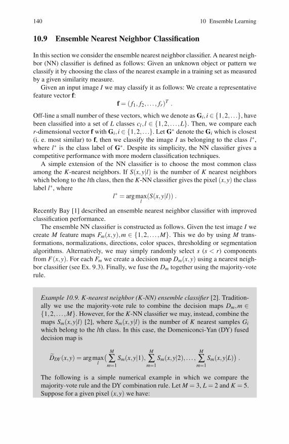
140 10 Ensemble Learning
10.9 Ensemble Nearest Neighbor Classification
In this section we consider the ensemble nearest neighbor classifier. A nearest neigh-bor (NN) classifier is defined as follows: Given an unknown object or pattern weclassify it by choosing the class of the nearest example in a training set as measuredby a given similarity measure.
Given an input image I we may classify it as follows: We create a representativefeature vector f:
f = ( f1, f2, . . . , fr)T .
Off-line a small number of these vectors, which we denote as Gi, i ∈ {1,2, . . .}, havebeen classified into a set of L classes cl , l ∈ {1,2, . . . ,L}. Then, we compare eachr-dimensional vector f with Gi, i ∈ {1,2, . . .}. Let G∗ denote the Gi which is closest(i. e. most similar) to f, then we classify the image I as belonging to the class l∗,where l∗ is the class label of G∗. Despite its simplicity, the NN classifier gives acompetitive performance with more modern classification techniques.
A simple extension of the NN classifier is to choose the most common classamong the K-nearest neighbors. If S(x,y|l) is the number of K nearest neighborswhich belong to the lth class, then the K-NN classifier gives the pixel (x,y) the classlabel l∗, where
l∗ = argmaxl
(S(x,y|l)) .
Recently Bay [1] described an ensemble nearest neighbor classifier with improvedclassification performance.
The ensemble NN classifier is constructed as follows. Given the test image I wecreate M feature maps Fm(x,y),m ∈ {1,2, . . . ,M}. This we do by using M trans-formations, normalizations, directions, color spaces, thresholding or segmentationalgorithms. Alternatively, we may simply randomly select s (s < r) componentsfrom F(x,y). For each Fm we create a decision map Dm(x,y) using a nearest neigh-bor classifier (see Ex. 9.3). Finally, we fuse the Dm together using the majority-voterule.
Example 10.9. K-nearest neighbor (K-NN) ensemble classifier [2]. Tradition-ally we use the majority-vote rule to combine the decision maps Dm,m ∈{1,2, . . . ,M}. However, for the K-NN classifier we may, instead, combine themaps Sm(x,y|l) [2], where Sm(x,y|l) is the number of K nearest samples Gi
which belong to the lth class. In this case, the Domeniconci-Yan (DY) fuseddecision map is
˜DDY (x,y) = argmaxl
(
M
∑m=1
Sm(x,y|1),M
∑m=1
Sm(x,y|2), . . . ,M
∑m=1
Sm(x,y|L))
.
The following is a simple numerical example in which we compare themajority-vote rule and the DY combination rule. Let M = 3, L = 2 and K = 5.Suppose for a given pixel (x,y) we have:

References 141
S1(x,y|1) =25
and S1(x,y|2) =35
,
S2(x,y|1) =25
and S2(x,y|2) =35
,
S3(x,y|1) =45
and S4(x,y|2) =15
.
The individual decision maps Dm(x,y) are
D1(x,y) = 2 , D2(x,y) = 2 and D3(x,y) = 1 .
The corresponding majority-vote and DY fused decision maps are:
˜Dma j(x,y) = argmaxl
(
M
∑m=1
Dm(x,y))
= 2 ,
˜DDY (x,y) = argmaxl
(
M
∑m=1
Sm(x,y|l),M
∑m=1
Sm(x,y|2), . . . ,M
∑m=1
Sm(x,y|L))
= 1 .
10.10 Further Reading
A modern book devoted to ensemble methods is [13]. For a recent survey of ensem-ble methods see [18]. For survey of real-world applications using ensemble learningsee [15]. For an additional application using ensemble learning see Sects. 16.3.
10.11 Software
STPRTOOL. A statistical pattern recognition toolbox. Authors: Vojtech Francand Vaclav Hlovac.
References
1. Bay, S.D.: Nearest neighbor classification for multiple feature subsets. Intell. DataAnaly. 3, 191–209 (1999)
2. Domeniconci, C., Yan, B.: Nearest neighbor ensemble. In: Proc. 17th Int. Conf. Patt.Recogn. (2004)
3. Giannarou, S., Stathaki, T.: Edge detection using quantitative combination of multipleoperators. In: IEEE Workshop on Signal Process. Systems Design and Implement, pp.359–364 (2005)
4. Hong, Y.: Random spatial sampling and majority voting based image thresholding. IEEESignal Process. Lett. (2008)

142 10 Ensemble Learning
5. Jarillo, G., Pedrycz, W., Reformat, M.: Aggregation of classifiers based on image trans-formations in biometric face recognition. Mach. Vis. Appl. 19, 125–140 (2008)
6. Ko, A.H.-R., Sabourin, R., de Britto Jr., A.S.: Compound diversity functions for ensem-ble selection. Int. J. Patt. Recogn. Art. Intell. 23, 659–686 (2009)
7. Krogh Vedelsby (1995)8. Liu, C.-L., Marukawa, K.: Normalization ensemble for handwritten character recogni-
tion. In: Proc. 9th Int. Workshop on Frontiers in Handwriting Recogn. (2004)9. Kuncheva, L.I.: Combining pattern Classifiers: Methods and Algorithms. John Wiley and
Sons, Chichester (2004)10. Mayo, M.: Random convolution ensembles. In: Ip, H.H.-S., Au, O.C., Leung, H., Sun,
M.-T., Ma, W.-Y., Hu, S.-M. (eds.) PCM 2007. LNCS, vol. 4810, pp. 216–225. Springer,Heidelberg (2007)
11. Melgani, F.: Robust image binarization with ensembles of thresholding algorithms. J.Elect. Imaging 15, 023010 (2006)
12. Nanni, L., Lumini, A.: Fusion of color spaces for ear authentication. Patt. Recogn. 42,1906–1913 (2009)
13. Okum, O., Valentini, G.: Supervised and Unsupervised Ensemble Methods and TheirApplications. Springer, Heidelberg (2008)
14. Orlov, N., Shamir, L., Macura, T., Johnston, J., Eckley, D.M., Goldberg, I.G.: WND-CHARM: Multi-purpose image classification using compound image transforms. Patt.Recogn. Lett. 29, 1684–1693 (2008)
15. Oza, N.C., Tumer, K.: Classifier ensembles: select real-world applications. Inf. Fusion 9,4–20 (2008)
16. Rohlfing, T., Maurer Jr., C.R.: Multiclassifier framework for atlas-based image segmen-tation. Patt. Recogn. Lett. 26, 2070–2079 (2005)
17. Sharifi, M., Fathy, M., Mahmoudi, M.T.: A classified and comparative study of edge de-tection algorithms. In: Proc. Int. Conf. Information Technology: Coding and Computing,pp. 117–120 (2002)
18. Rokach, L.: Taxonomy for characterizing ensemble methods in classification tasks: Areview and annotated bibliography. Comp. Stat. Data Anal. 53, 4046–4072 (2009)
19. Wang, H., Suter, D.: False-peaks-avoiding mean shift method for unsupervised peak-valley sliding image segmentation. In: Proc 7th Digital Image Computing: Techniquesand Applications, pp. 581–590 (2003)

Chapter 11Re-sampling Methods
Abstract. The subject of this chapter are the re-sampling methods which are a spe-cial set of ensemble learning techniques. In the context of image fusion the re-sampling methods create an ensemble of input images Ik,k ∈ {1,2, . . . ,K}, froma single base image I∗. In this chapter we shall concentrate on two important re-sampling methods: bootstrapping and boosting.
11.1 Introduction
In the context of image fusion, we use the term ensemble learning to denote thefusion of K input images Ik,k ∈ {1,2, . . . ,K}, where the Ik are all derived from thesame base image I∗. In the previous chapter we constructed the Ik by applying differ-ent signal processing algorithms to I∗. These algorithms include image transforma-tions, normalizations, feature extraction, thresholding and segmentation algorithms.In this chapter we consider a different (re-sampling) approach in which we applyan ensemble of K (fixed) classifiers Ck,k ∈ {1,2, . . . ,K} to I∗. In the re-samplingmethod the Ck are obtained by training the parameters of a parametric classifier S onre-sampled training data T ∗. If Dk denotes the decision map obtained by applyingCk to I∗, then we fuse the Dk,k ∈ {1,2, . . . ,K}, together to obtain a fused decisionmap ˜D. In general, ˜D is more accurate than any one of the Dk.
The strength of the re-sampling method is that it allows for a systematic genera-tion of a virtually unlimited number of classifiers Ck and the corresponding decisionmaps Dk in a natural way.
We start with bootstrapping, which is perhaps the most widely used re-samplingmethod.
11.2 Bootstrapping
Bootstrapping is a basic re-sampling technique in which we generate which an en-semble of K fixed classifiers Ck,k∈ {1,2, . . . ,K}, given a base training data base T ∗.

144 11 Re-sampling Methods
Given T ∗ we generate K bootstrapped training sets Tk,k ∈ {1,2, . . . ,K}, by samplingT ∗ with replacement (see Ex. 3.10). Then, given a parametric classifier S we cre-ate an ensemble of fixed classifiers Ck,k ∈ {1,2, . . . ,K}, by separately training S oneach training set Tk
[1]. If we apply Ck to the test image I∗ we obtain a decision mapDk. Finally, we obtain a fused decision map ˜D by fusing the Dk together:
˜D = f (D1,D2, . . . ,DK) ,
where f is an appropriate fusion operator.In many cases we use the majority vote rule to fuse the Dk. In this case the com-
bination of bootstrapping and majority vote rule is known as “bagging”. In generalbagging is useful when the Ck are weak. By this we mean that the performance ofthe classifier is slightly better than random but is unstable: changes in the trainingdata cause significant changes in the fixed classifier.
We illustrate the concept of bagging on two different applications. The first ap-plication illustrates the traditional use of bagging a supervised classifier. The secondapplication illustrates a recent development in which we use bagging in an unsuper-vised classifier or clustering algorithm.
11.3 Face Recognition with Bagging
We consider face recognition in an unconstrained environment where the appear-ance of a given face may vary due to changes in lighting, pose and facial expression[5]. In many face recognition applications, only a small number of training samplesfor each subject are available. These samples are not able to capture all the facialappearance variations. By bootstrapping the training set T ∗ we generate several sub-sets Tk,k ∈ {1,2, . . . ,K}, of samples from the original training dataset. Each subsetTk is then used to train a classifier Ck.
Given a test face we classify it using the classifiers Ck,k ∈ {1,2, . . . ,K}. If Dk isthe decision obtained with the classifier Ck, then we obtain a fused decision ˜D byfusing the Dk together using the majority-vote rule. Blu and Jain [5] found the useof bootstrapping made a substantial improvement in the face recognition accuracy:increasing from 81% to 88.7%.
11.4 Bagged Nearest Neighbor Classifier
The nearest neighbor (NN) classifier (see Sect. 10.9) is simple but very effectiveclassifier which is widely used in many real-world classification systems. It is not,however, a weak classifier, and consequently (conventional) bagging will not im-prove its performance. However, by creating bootstrapped training sets which are
1 A parametric classifier is a classifier which has free parameters in it. Optimal values forthese parameters are found by training the classifier on a training set. Once the parametervalues are specified we have a fixed classifier.

11.5 Bagged K-means Clustering 145
smaller in size than the original training set, we “weaken” the NN classifier whichcan now be bagged.
Example 11.1. Bagged Nearest Neighbor Classifier [3]. Given a base trainingset T ∗ containing M images ym,m ∈ {1,2, . . . ,M}, we create a set of K boot-strapped training sets Tk,k ∈ {1,2, . . . ,K}, where each training set Tk containsN images which are selected by randomly sampling T ∗ with replacement andN ≈ 0.7M.
Given a test image I we classify it using the NN classifier on each boot-strapped training set Tk,k ∈ {1,2, . . . ,K}. Suppose the NN classification ob-tained with the kth training set is a decision label l:
Dk = l ,
then the bagged NN classification of I is
˜D = l ifK
∑k=1
δ (Dk, l) >K2
,
where
δ (a,b) ={
1 if a = b ,0 otherwise .
11.5 Bagged K-means Clustering
Traditionally, re-sampling methods are used in supervised learning applications inorder to improve classification accuracy. Recently re-sampling methods have beenused to improve unsupervised clustering algorithms.
In this context we use bagging to generate and aggegrate multiple clusteringsand to assess the confidence of cluster assignments for individual observations. Themotivation is to reduce the variability in the partitioning results via averaging.
Given an input base image I∗ we may segment it into a L label decision imageD∗ using a K-means clustering algorithm (see Ex. 6.8). Let G1,G2, . . . ,GK denoteL cluster centers or cluster gray-levels. Then each pixel gray-level gm ≡ I∗(m) isassigned to a given cluster:
δml ={
1 if gm is assigned to Gl ,0 otherwise .
We then use the assignment matrix δml to create the decision image D∗:
D∗(m) = l if δml = 1 .

146 11 Re-sampling Methods
The K-means algorithm attempts to find the set of cluster centers Gl, l ∈{1,2, . . . ,L},such that the total error is a minimum:
(G1,G2, . . . ,GL) = argminGk
M
∑m=1
L
∑k=1
δmk|gm−Gk| ,
using the following iterative procedure. In each iteration we calculate the assign-ment matrix δml using the cluster centers Gl calculated in the previous iteration.The cluster centers are then re-calculated using the new assignment matrix. Theentire process for T iterations is:
for t = 1 : Tfor m = 1 : M
δ (t)mk =
{
1 if |gm−G(t−1)l |= minh |gm−G(t−1)
h |0 otherwise
endfor l = 1 : L
G(t)l = ∑M
m=1 δ(t)ml gm/∑M
m=1 δ(t)ml
endend
Dudoit and Fridlyand [1] show how we may improve the performance of the clusteralgorithm by bagging.
Example 11.2. Bagged K-means Clustering Algorithm [1]. The steps in thebagged K-means clustering algorithm are:
1. Transform the base image I∗ into a column vector I∗(m),m ∈ {1,2, . . . ,M}2. Form K bootstrapped column vectors I(k)(m),k ∈ {1,2, . . . ,K},m ∈{1,2, . . . ,M} by sampling I∗ with replacement.
3. Train the K-means cluster algorithm on each bootstrapped column vector
I(k), i. e. learn L cluster centers G(k)l , l ∈ {1,2, . . . ,L}.
4. For each k, permute the labels l so that G(k)1 < G(k)
2 < .. . < G(k)L . This en-
sures the semantic equivalence of the labels l (see Ex. 5.5 ).
5. For each set of cluster centers G(k)l ,k ∈ {1,2, . . . ,K}, classify the pixels in
I∗:D(k)(m) = argmin
l(|I∗(m)−G(k)
l |) .
6. For each pixel m,m ∈ {1,2, . . . ,M}, form a bagged decision ˜D(m) using amajority-vote rule:

11.6 Boosting 147
˜D(m) = l if ∑Kk=1 δ (D(k)(m), l))≥ K
2 ,
where
δ (a,b) ={
1 if a = b ,0 otherwise .
11.6 Boosting
Boosting is closely related to bagging except the training sets Tk,k ∈ {1,2, . . . ,K},are no longer independent, instead they are created sequentially. If Ck denotes theclassifier which is trained on Tk, then Tk+1 is created in accordance with the classi-fication accuracy obtained with Ck.
Adaboosting is probably the most successful boosting algorithm. It creates an en-semble of fixed classifiersCk,k∈{1,2, . . . ,K}, as follows. Let T∗(i), i∈{1,2, . . . ,N},denote the individual samples in T∗. At the kth iteration, each sample T∗(i) is assigneda weight wk(i). Together, the training samples T∗(i) and the weights wk(i) constitute aweighted training set Tk. At the kth iteration we create a fixed classifier Ck by traininga parametric classifier S on the weighted training set Tk. For the next iteration (k+1)we update wk(i), i ∈ {1,2, . . . ,N}, by increasing the weight of wk(i) if Ck incorrectlyclassifies T ∗(i) and decreasing the weight of wk(i) if Ck correctly classifies T ∗(i).
The following is the pseudo-code for the two-class adaboost algorithm:
Example 11.3. Adaboost Algorithm
Initialize w0(i) = 1/N, i ∈ {1,2, . . . ,N}For k = 0 : K
Generate Ck by training S on a weightedtraining set Tk
Find samples T ∗(i) which are misclassified by Ck:
δk(i) ={
1 if Ck misclassifies T ∗(i)0 otherwise.
Calculate EK and βk:Ek = ∑N
i=1δk(i)wk(i), βk = Ek/(1−Ek)Update the weight vector:
wk+1(i) = wk(i)(δk(i)+ (1− δk(i))βk)Normalize wk+1: wk+1(i) = wk+1(i)/∑N
i=1 wk+1(i)end
Given the classifiers Ck,k ∈ {1,2, . . . ,K}, we classify a test sample as follows:Let Dk be the classification of the test sample obtained with the classifier Ck. Then

148 11 Re-sampling Methods
we fuse the Dk using a weighted majority-vote rule, where the weight given to eachclassifier Ck is proportional to its accuracy on the weighted training set used to trainCk. The final classification of the test sample is ˜D:
˜D = l ifK
∑k=1
log(1/βk)δ (Dk, l)≥ 12
K
∑k=1
log(1/βk) .
where
δ (a,b) ={
1 if a = b ,0 otherwise .
Adaboost is widely used in classification applications. Since its introduction in 1997[2] it has established itself as a high-performance general purpose classifier. How-ever, in noisy situations, such as those with label noise, the adaboost algorithm mayperform poorly. In this case we may use the ave2boost algorithm. This is a modifiedversion of adaboost specifically designed for noisy situations. In ave2boost we reg-ulate how the weight vector wk is updated and we modify the weighted-vote rule.For the sake of completeness we give the pseudo-code for ave2boost:
Example 11.4. Ave2boost Algorithm [8].
Initialize w0(i) = 1/N, i ∈ {1,2, . . . ,N}For k = 0 : K
Generate Ck by training S on weightedtraining set Tk
Find samples T ∗(i) which are misclassified by Ck:
δk(i) ={
1 if Ck misclassifies T ∗(i)0 otherwise.
Calculate Ek,βk and γk:Ek = ∑N
i=1δk(i)wk(i), βk = Ek/(1−Ek), γk = 2(1−Ek)k+12Ekk+1
Update the weight vector:wk+1(i) = wk(i)(δk(i)+ (1− δk(i))βk)
Calculate regularization factors:vk+1(i) = wk+1(i)/∑N
i=1 wk+1(i)Normalize wk+1: wk+1(i) = (kwk+1(i)+ vk+1(i))/(k + 1)
endClassify test sample with each Ck:
Dk = l if Ck identifies test sample as belongingto the lth class
Final classification of test sample is:˜D = l if ∑K
k=1 log(1/(βkγk))δ (Dk, l) ≥ 12 ∑
Kk=1 log(1/(βkγk))
where δ (Dk, l) = 1 if Dk = l, otherwise δ (Dk, l) = 0.

11.8 Boosted Object Detection 149
11.7 Viola-Jones Algorithm
The conventional adaboost algorithm uses only one parametric classifier S. Violaand Jones (VJ) [10] remove this restriction and use instead M parametric classi-fiers Sm,m ∈ {1,2, . . . ,M}. In each iteration k,k ∈ {1,2, . . . ,K}, we select one fixedclassifier Ck as follows:
1. Generate M fixed classifiers ck,m,m∈ {1,2, . . . ,M}, by training Sm,m∈ {1,2, . . . ,M}, on the weighted training set Tk.
2. Select the fixed classifier with the smallest weighted error:
Ck = ck,m if m = argminm
N
∑i=1δk,m(i)wk(i) ,
where
δk,m(i) ={
1 if ck,m misclassifies T ∗(i) ,0 otherwise .
11.8 Boosted Object Detection
The VJ algorithm was originally developed for real-time object detection. In thisapplication the number of parametric classifiers Sm,m ∈ {1,2, . . . ,M}, is very large.For example, in typical application concerning face detection in an input image, M≈180000 and special attention must therefore be paid to generating and efficientlytraining the Sm.
The boosted object detection algorithm works as follows. We create N trainingsamples T ∗(i), i∈{1,2, . . . ,N}, by dividing several training images into overlappingblocks of size L×L. Each block Bi constitutes a training sample T ∗(i), where
y(i) ={
1 if Bi contains an object ,0 otherwise .
In each iteration k of the algorithm, we probe the blocks Bi, i ∈ {1,2, . . . ,N}, with aL×L ternary mask φm (Fig. 11.1) and compare the result to a threshold θ :
dk,m(i) ={
1 if p∑(x,y) φm(x,y)B(x,y)≥ pθ ,0 otherwise .
where p is a polarity variable (p=−1 or +1) which determines if the (∑(x,y) φk,m(x,y)×B(x,y)) should be greater, or smaller, than θ . We fix the polarity variable p and thethreshold θ by minimizing the weighted error:
ek,m =N
∑i=1
wk(i)|dk,m(i)− y(i)| .

150 11 Re-sampling Methods
(a) (b) (c)
(d) (e)
(f) (g)
Fig. 11.1 (a)-(e) Show five basic masks which contain only −1 and +1 values. (f) Showsa ternary mask φm obtained by placing the first basic mask in a block of zeros. (g) Show aternary mask φl obtained by scaling the first basic mask and placing it in a block of zeros. Inthe figure, white, black, and gray stand, respectively, for values of +1, −1 and 0.

11.8 Boosted Object Detection 151
The following example is the pseudo-code for the Viola-Jones algorithm.
Example 11.5. Viola-Jones Object Detection Algorithm [6, 10].
1. Extract the features fm(i) = ∑(x,y) φm(x,y)Bi(x,y),m ∈ {1,2, . . . ,M}, foreach training block B(i), i ∈ {1,2, . . . ,N}.
2. Initialize the weight w1(i) for each training block i:
w1(i) ={
1/(2Ntrue) if B(i) contains an object ,1/(2Nf alse) if B(i) does not contain an object ,
where Ntrue is the number of training blocks which contain an object andNf alse is the number of training blocks which do not contain an object.
3. For k = 1 : K perform the following:a. Normalize the weights wk(i):
wk+1(i) = wk(i)/N
∑i=1
wk+1(i) .
b. For each features fm create a fixed classifier ck,m by training Sm on theweighted error:
ek,m =N
∑i=1
wk(i)|dk,m(i)− y(i)| ,
c. Feature selection. Choose the fixed classifier Ck with the lowestweighted error Ek:
Ck = ck,m
Ek = ek,m
}
if m = argminn
(ek,n) ,
d. Update the weights wk(i):
wk+1(i) = wk(i)β(1−Δk(i))k .
where βk = Ek/(1−Ek) and
Δk(i) ={
1 if Ck incorrectly classifies B(i) ,0 otherwise .
4. For a test block B we separately classify it using the fixed classifiers Ck,k ∈{1,2, . . . ,K}. If Dk,k ∈ {1,2, . . . ,K}, are the corresponding decisions, thenwe combine the Dk to obtain a fused decision ˜D:
˜D ={
1 if ∑Kk=1αkDk ≥ ∑K
k=1αk/2 ,0 otherwise ,
where αk = log(1/βk).

152 11 Re-sampling Methods
For real-time processing, the parametric classifiers Sm are constructed by scaling abasic binary mask (containing only the values −1 and +1) and placing it anywherein a L×L background of zeros. This method of construction facilitates real-time pro-cessing by using method of integral images which we now explain in the followingexample.
Example 11.6. Integral Image. Given an L×L image block B with pixel gray-levels B(x,y),x,y ∈ {1,2, . . . ,L}, we pre-compute the following sum:
IΣ (x,y) =x
∑u=1
y
∑v=1
B(u,v) .
Then the feature value f (B) =∑(x,y) B(x,y)φ(x,y), corresponding to the maskφ shown in Fig. 11.2 may be efficiently calculated in four operations:
f (B) = IΣ (x2,y2)− IΣ(x1,y1)− (IΣ(x4,y4)− IΣ(x3,y3)) .
(x1,y
1)
(x2,y
2)
(x4,y
4)
(x3,y
3)
Fig. 11.2 Shows a ternary mask φ obtained by placing a binary mask in a block of zeros. Inthe figure white, black and gray stand, respectively, for values of +1, −1 and 0. The top left-hand corner and bottom right-hand corner of the +1 block are (x1,y1) and (x2,y2). Similarly,the top left-hand corner and bottom right-hand corner of the −1 block (x3,y3) and (x4,y4).
11.9 Software
STPRTOOL. A statistical pattern recognition toolbox. Authors: Vojtech Francand Vaclav Hlovac.

References 153
11.10 Further Reading
A modern book devoted to ensemble methods is [7]. Ref. [4] is a detailed report onimplementation of the Viola-Jones algorithm for real-time object detection. For arecent extension of the Viola-Jones algorithm for object detection see [9]
References
1. Dudoit, S., Fridlyand, J.: Bagging to improve the accuracy of a clustering procedure.Bioinformatics 19, 1090–1099 (2003)
2. Freund, Y., Schapire, R.E.: Decision-theoretic generalization of on-line learning and anapplication to boosting. J. Comp. System Sci. 55, 119–139 (1997)
3. Hall, P., Samworth, R.J.: Properties of bagged nearest neighbor classifiers. J. R. Statist.Soc. 67B, 363–379 (2005)
4. Jensen, O.H.: Implementing the Viola-Jones face detection algorithm. MSc thesis, Tech-nical University of Denmark (2008)
5. Lu, X., Jain, A.K.: Resampling for Face Recognition. In: Kittler, J., Nixon, M.S. (eds.)AVBPA 2003. LNCS, vol. 2688. Springer, Heidelberg (2003)
6. Martins, R., Pina, P., Margques, J.S., Silveira, M.: Crater detection by a boosting ap-proach. IEEE Geosci. Remote Sensing Lett. 6, 127–131 (2009)
7. Okum, O., Valentini, G.: Supervised and Unsupervised Ensemble Methods and TheirApplications. Springer, Heidelberg (2008)
8. Oza, N.C.: Ave2boost: boosting for noisy data. In: Roli, F., Kittler, J., Windeatt, T. (eds.)MCS 2004. LNCS, vol. 3077, pp. 31–40. Springer, Heidelberg (2004)
9. Pavani, S.-K., Delgado, D., Frangi, A.F.: Haar-like features with optimally weighted rect-angles for rapid object detection. Patt. Recogn. (in print, 2009)
10. Viola, P., Jones, M.: Robust real-time face detection. Int J. Comp. Vis. 57, 137–154(2004)

Chapter 12Image Thresholding
Abstract. The subject of this chapter is image thresholding in which we transforman input image, A, into a binary image B, where the pixel gray-levels in B are re-stricted to {0,1}. If am is the gray level of the mth pixel in A, then the correspondingvalue in B is
bm ={
1 if am ≥ tm ,0 otherwise ,
where tm is the threshold value for the mth pixel. The thresholds tm,m∈ {1,2, . . . ,M},may all be equal to a global threshold tG or they may vary locally (i. e. from pixel topixel). In this chapter we shall concentrate on unsupervised thresholding methods.These are thresholding algorithms in which we only use information contained in thecurrent input image to calculate tm and tG.
12.1 Global Thresholding
Let A denote a given input image, where am denotes the gray-level of the mth pixel.Then the pixels in the image are divided into two groups: “low” intensity pixelswhose gray-levels are less than, or equal to, a threshold t and “high” intensity pixelswhose gray-levels are greater than t. We follow [12] and categorize the thresholdingmethods into five groups as follows:
Histogram-based Methods. These methods analyze the shape and features of theimage histogram.
Cluster-based Methods. These methods cluster the pixel gray-levels into twoparts as background and foreground pixels.
Entropy-based Methods. The methods use the entropy of the histogram or cross-entropy between input image and the thresholded image to find an optimalthreshold.

156 12 Image Thresholding
Object Attribute-based methods. The methods use a measure of similarity be-tween the gray-level and the binarized images.
Spatial-based Methods. The methods use a higher-order probability distributionto model the correlation between pixels.
In some applications we find it useful to modify the input image before thresholding.The following example describes one such application involving the estimation ofraindrop sizes.
Example 12.1. Histogram Modification [13]. Rainfall estimates often requirean estimate of the distribution of raindrop sizes. Unfortunately image irreg-ularities mean the size estimates are often noisy and inaccurate. In [13] theimage irregularities are reduced by applying the following iterative histogrammodification algorithm to the raindrop images.
The algorithm iteratively sharpens the peaks of the input image histogramby considering the number of pixels Hi having a particular gray-level i andcomparing it with Hi:
Hi =1
2R
(
i−1
∑k=i−R
Hi +i+R
∑k=i+1
Hi
)
,
where Hi is the average number of pixels in the neighboring R bins on eitherside of i. Whenever Hi > Hi, we shift xHl� pixels from the lth bin to theneighboring bin nearest to the ith bin, where
x =Hi− Hi
Hi.
12.2 Statistical Algorithms
Many of the global thresholding algorithms are statistical in nature. In this case, thethreshold t is found by analyzing the image histogram H = (H0,H1, . . . ,HK−1)T ,or equivalently, the probability distribution p = (p0, p2, . . . , pK−1)T , where Hk isthe number of pixels in the input image whose gray levels are equal to k [1] andpk = Hk/∑K−1
l=0 Hl .Fig. 12.1 shows binary images Bk,k ∈ {1,2, . . . ,K}, obtained by thresholding an
input image I using K different global thresholding algorithms.
1 For an 8-bit deep input image the gray-levels are 0,1, . . . ,255, i. e. K = 256.

12.2 Statistical Algorithms 157
(a) (b)
(c) (d)
(e) (f)
Fig. 12.1 (a) Shows an input image I. (b)-(e) Shows the binary image obtained by threshold-ing I using the Otsu, Kittler-Illingsworth, Kapur and Tsai thresholding algorithms. (f) Showsthe binary image obtained by thresholding I using a maximum likelihood algorithm in whichwe assume a mixture of two Gaussian distributions [1].

158 12 Image Thresholding
12.2.1 Ridler-Calvard
Ridler and Calvard [10] describe an iterative heuristic thresholding technique. Theinitial threshold, t, is set equal to the mean pixel gray-level μ:
μ =K
∑k=0
kHk/K
∑k=0
Hk .
Thereafter, the threshold value tk for the kth iteration is given by:
tk =μ0(tk)+ μ1(tk)
2,
where μ0(tk) and μ1(tk) are, respectively, the mean gray-levels of the pixels whichlie below and above the threshold tk.
12.2.2 Otsu
According to Otsu [9] we select a threshold t which minimizes the within-groupvariance σ2
W (t) of the pixels. Mathematically, σ2W (t) is defined as follows:
σ2W (t) = P0(t)σ2
0 (t)+ P1(t)σ21 (t) ,
where P0(t) and P1(t) are, respectively, the proportion of pixel gray-levels which liebelow, and above, the threshold t and σ2
0 (t) and σ21 (t) are, respectively, the variance
of the pixel gray-levels which lie below, and above, the threshold t. The optimumthreshold may be found by an exhaustive search. In Ex. 6.6 we illustrate the actionof the Otsu algorithm to segment an input image into areas of background and areasof foreground.
For an efficient method of implementating the Otsu algorithm see [4].
12.2.3 Kittler-Illingworth
According to Kittler and Illingworth [7] we select a threshold t which minimizes acriterion J(t), where
J(t) = 1 + 2(P0(t) lnσ0(t)+ P1 lnσ1(t))−2(P0(t) lnP0(t)+ P1(t) ln P1(t)) .
where P0(t) and P1(t) are, respectively, the proportion of pixel gray-levels whichlie below and above the threshold t. If the below threshold and the above thresh-old pixels each follow a Gaussian distribution, then the criterion J(t) represents theaverage pixel classification error rate. As the threshold t is varied, the parametersP0(t),P1(t),σ2
0 (t) and σ21 (t) change. The problem of minimum error threshold se-
lection is reduced to computing J(t) for all t, and finding its minimum value.Note. Even if the assumption of a bimodal normal distribution is valid , the model
parameters are biased estimates of the true values, as the tails of the overlapping

12.2 Statistical Algorithms 159
distributions are truncated. Thus, the correctness of the estimated threshold relieson this overlap being small. However, the most challenging images are those wherethe histograms do not have two well separated modes [3].
12.2.4 Kapur
According to Kapur [6] we select a threshold t which maximizes the sum of theentropies of pixel gray-levels which lie below the threshold t and which lie abovethe threshold t. Mathematically, the sum of the entropies is
ψ(t) = ln(P0(t)P1(t))+Ht
P0(t)+
HG−Ht
P1(t),
where
Ht = −t
∑k=0
pk ln pk ,
HG = −K−1
∑k=0
pk ln pk .
The discrete value of t which maximizes ψ(t) is the threshold value which maxi-mizes the information between object and background.
12.2.5 Tsai
According to Tsai [14] we select a threshold t such that the binary image has thesame first three moments as the input image, where the ith moment of the image I is
mi =K−1
∑k=0
ki pk ,
and, by definition, m0 = 1.
Example 12.2. Change Detection in Remotely Sensed Imagery [8]. The mostcommon methodology to carry out an unsupervised change detection in re-motely sensed imagery is to compare two spatially aligned multitemporal re-mote sensing images I1(m,n) and I2(m,n) taken at two different dates overthe same geographical area. The result of the comparison is a binary imageB(m,n) where
B(m,n) ={
1 if the pixel (m,n) is classified as “changed” ,0 otherwise .
(12.1)

160 12 Image Thresholding
One way of generating B is to threshold the difference image D = |I1− I2| us-ing one of the above global thresholding algorithms. A more powerful methodis to match the local gray-level distributions in the two images: For each pixel(m,n) we establish a window W of size (2L+1)×(2L+1) centered on (m,n).Let H1 and H2 denote, respectively, the local distributions, or histograms, ofthe pixel gray-levels I1(i, j) and I2(i, j),(i, j) ∈W . We then compare H1 andH2 using an appropriate similarity measure (see Chapt. 14). We often use themutual information MI(H1,H2) or the Kullback-Leibler distance KL(H1,H2)for this purpose.
For a method of combining multiple thresholded images using an unsupervisedweighted majority vote rule see Ex. 10.7.
12.3 Local Thresholding
In general local thresholding algorithms work by moving a sliding window overthe input image. In each window we calculate a threshold t using one of the aboveglobal thresholding algorithms. Then t is applied to the center pixel of the window.
However this approach suffers from the drawback that there is no principledmethod for choosing the local window size. A recent alternative method is the fol-lowing “ensemble-learning” algorithm (see Sect. 10.7) which may be used to con-vert the global thresholding algorithms into local algorithms.
Given an input image I we randomly select K image patches from I. The size andlocation of the image patches is random and the patches may overlap. Thus a givenpixel (m,n) may be present in L image patches, where 0≤ L≤K. We threshold eachimage patch using a global thresholding algorithm. Then for each pixel (m,n) wecalculate the number of times it has a label of one. If the number of times is greaterthan, or equal to, L/2, then we set B(m,n) equal to one, otherwise B(x,y) = 0.
12.4 Software
HISTHRESH. HistThresh is a matlab toolbox for global image thresholding. Au-thor is Antti Niemisto.
12.5 Further Reading
Recently the expectation-maximization (EM) algorithm has been used for imagethresholding assuming the foreground and background pixels follow a given distri-bution. In [1] the foreground and background pixels are assumed to follow a general-ized Gaussian distribution. A comprehensive survey of image thresholding methodsis [12]. A survey of entropy and relative entropy thresholding methods is [2]. Twoearlier reviews are: [5] and [11].

References 161
References
1. Bazi, Y., Bruzzone, L., Melgani, F.: Image thresholding based on the EM algorithm andthe generalized Gaussian distribution. Patt. Recogn. 40, 619–634 (2007)
2. Chang, C.-I., Du, Y., Wang, J., Guo, S.-M., Thouin, P.D.: Survey and comparative anal-ysis of entropy and relative entropy thresholding techniques. IEE Proc. Vis. Image Sig.Process. 153, 837–850 (2006)
3. Cho, S., Haralick, R., Yi, S.: Improvement of Kittler and Illingworth’s minimum errorthresholding. Patt. Recogn. 22, 609–618 (1989)
4. Dong, L., Yu, G., Ogunbona, P., Li, W.: An efficient iterative algorithm for image thresh-olding. Patt. Recogn. Lett. 29, 1311–1316 (2008)
5. Glasbery, C.A.: An analysis of histogram-based thresholding algorithms. Comp. Vis.Graphics Image Process. 55, 532–537 (1993)
6. Kapur, J.N., Sahoo, P.K., Wong, A.K.C.: A New Method for Gray-Level Picture Thresh-olding Using the Entropy of the Histogram. Comp. Vis. Graphics Image Process. 29,273–285 (1985)
7. Kittler, J., Illingworth, J.: Minimum error thresholding. Patt. Recogn. 19, 41–47 (1986)8. Melgani, F., Bazi, Y.: Markovian fusion approach to robust unsupervised change detec-
tion in remotely sensed imagery. IEEE Geosci. Remote Sensing Lett. 3, 457–461 (2006)9. Otsu, N.: A threshold selection method from gray-level histogram. IEEE Trans. Syst.
Man Cyber. 9, 62–66 (1979)10. Ridler, T.W., Calvard, S.: Picture thresholding using an interative selection method. IEEE
Trans. Syst. Man Cyber. 8, 630–632 (1978)11. Sahoo, P.H., Soltani, S., Wong, A.K.C.: A survey of thresholding techniques. Comp. Vis.
Graphics Image Process. 41, 233–260 (1988)12. Sezgin, M., Sankur, B.: Survey over image thresholding techniques and quantitative per-
formance evaluation. J. Elect. Imag. 13, 146–165 (2004)13. Sivasubramanian, N.A., Saylor, J.R.: Application of a histogram modification algorithm
to the processing of raindrop images. Opt. Engng. 47, 037011-1–037011-10 (2008)14. Tasi, W.: Moment-preserving thresholding: a new approach. Comp. Vis. Graphics Image
Process. 29, 377–393 (1985)

Chapter 13Image Key Points
Abstract. The subject of this chapter is image key points which we define as a dis-tinctive point in an input image which is invariant to rotation, scale and distortion.In practice, the key points are not perfectly invariant but they are a good approxima-tion. To make our discussion more concrete we shall concentrate on two key pointalgorithms: SIFT and SURF and their use in spatial alignment.
13.1 Scale-Invariant Feature Transform
The scale-invariant feature transform [5] (SIFT) algorithm provides a robust methodfor extracting distinctive features from an input image I which are invariant to ro-tation, scale and distortion. These points (known as “key-points”) are found by de-tecting local extrema in a multi-scale representation of I:
{D(m,n|σ1),D(m,n|σ2), . . . ,D(m,n|σK)} , (13.1)
where D(m,n|σk) is the difference-of-Gaussian (DoG) representation of I at a scaleσk:
D(m,n|σk) = I(m,n)⊗G(σk)− I(m,n)⊗G(σk+1) ,
and I(m,n)⊗G(σk) denotes the convolution of I(m,n) with the two-dimensionalzero-mean Gaussian G(σk) and σk+1 = 21/3σk. The parameter K is specified by theuser and is based on the maximum width in pixels.
The local extrema in (13.1) are defined as points (m,n|σk) for which D(m,n|σk)is greater than its 26 neighbors. This includes eight immediate neighbors fromthe D(p,q|σk) and nine neighbors from D(p,q|σk+1) and nine neighbors fromD(p,q|σk−1). This is followed by accurate interpolation of scale space using theTaylor series expansion upto a second degree of D(m,n|σk) in the neighborhood of(m,n) and σk.
Stability of the extrema is further ensured by rejecting key-points with low con-trast and key points localized along edges. For a descriptor of the key-point, anorientation histogram is computed of the area surrounding the key-point. Gradient

164 13 Image Key Points
magnitude and the weight of a Gaussian window originating at the key-point add tothe value of each sample point within the considered region.
Mathematically the SIFT operator is computed by partitioning the image regionsurrounding each detection key point into a 4×4 grid of subregions, and computingan orientation histogram of 8 bins in each sub-region (Fig. 13.1).
Fig. 13.1 Shows the formation of the SIFT descriptor for a key-point located at (m,n). In thefigure we show the 4×4 sub-regions with their orientation vectors.
The grid is square, with the x-axis oriented along the key-point gradient direc-tion and the width of the grid being approximately 12 times the detected scale ofthe key-point. Within each subregion, the gradient orientation of each pixel is en-tered into the orientation histogram, with weighted vote proportional to the gradientmagnitude. A normalized 128 component vector is formed by concatenating the 16region containers.
13.1.1 Hyperspectral Images
The SIFT operator has been extended to color images [1, 3] and hyperspectral im-ages [6] as follows. Given a hyperspectral image
I(m,n|l), l ∈ {1,2, . . . ,L} ,
with L bands, we separately perform the DoG operation on each band [6]:
D(m,n|l) = I(m,n|l)⊗G(σk)− I(m,n|l)⊗G(σk+1) ,
and then combine the Dl(m,n|l) using a non-linear function f :

13.3 Complex Wavelet Transform 165
˜D(m,n) = f (D(m,n|1),D(m,n|2), . . . ,D(m,n|L)) .
The function ˜D(m,n) is then processed in the same way as D(m,n) is processedin the conventional SIFT operator. In hyperspectral images the number of bands Lmay be one or two hundred. In this case, we may reduce the computational load byreducing the number of bands by applying a PCA operator [6].
For the non-linear function f we may use several different alternatives. Two sim-ple functions are:
˜D(m,n) =
⎧
⎨
⎩
∑Ll=1 |D(m,n|l)|/L ,
∑Ll=1 wl |D(m,n|l)|/∑L
l=1 wl ,
where
wl ={
1 if D(m,n|l) > median(D(m,n|1),D(m,n|2), . . . ,D(m,n|L)) ,0 otherwise .
13.2 Speeded-Up Robust Feature
The speeded-up robust feature (SURF) [2] algorithm is a variation of the SIFT al-gorithm. Its major difference includes using a Hessian matrix:
H(x,y) =(
Ixx(x,y|σ) Ixy(x,y|σ)Ixy(x,y|σ) Iyy(x,y|σ)
)
,
as an interest point detector, where Ixx(x,y|σ) is the convolution of the Gaussiansecond-order derivative ∂ 2G(σ)/∂x2 with the input image at (x,y) and similarlyfor Ixy(x,y|σ) and Iyy(x,y|σ). SURF uses integral images (see Ex. 11.6) to calculateH(x,y). This makes SURF much faster than SIFT but with comparable performance.
13.3 Complex Wavelet Transform
The dual-tree complex wavelet transform (see Chapt. 8) provides us with a radicallydifferent type of key-point detector [4].
Example 13.1. Dual-Tree Complex Wavelet Transform for Key-Point Detec-tion [4]. The dual-tree CWT decomposition of an M×N input image I re-sults in a decimated dyadic decomposition into L levels, where each levell is a complex image of size M/2l ×N/2l . Thus at each (decimated) loca-
tion (i, j) in level l, we have a set of six complex coefficients: y(m)l (i, j) ≡
ρ (m)l eiθm ,m ∈ {1,2, . . . ,6}, corresponding to the M = 6 orientations θm ={15o,45o,75o,105o,135o,165o}. We may define a key-point energy measureEl(i, j) as

166 13 Image Key Points
El(i, j) = α l(M
∏m=1
ρ (m)l
)β,
where α and β are two parameters whose recommended values are: α = 1and β = 0.25. We then use the El(i, j) values as indicating the presence, orotherwise, of a key-point at level l and decimated location (i, j).
13.4 Software
SIFT. Matlab routine for SIFT operator. Author: Andrea Vedaldi.
References
1. Abdel-Hakim, A.E., Farag, A.A.: CSIFT: A sift descriptor with color invariant character-istics. In: Proc. IEEE Conf. Comput. Vis. Pattern Recog., vol. 2, pp. 1978–1983 (2006)
2. Bay, H., Tuytelaars, T., Van Gool, L.: SURF: Speeded up robust features. In: Leonardis,A., Bischof, H., Pinz, A. (eds.) ECCV 2006. LNCS, vol. 3951, pp. 404–417. Springer,Heidelberg (2006)
3. Brown, M., Lowe, D.: Invariant features from interest point groups. In: Proc. Brit. Mach.Vis. Conf., pp. 656–665 (2002)
4. Fauqueur, J., Kingsbury, N., Anderson, R.: Multiscale key-point detection using the dual-tree complex wavelet transform. In: Proc. Int. Conf. Image Process. (2006)
5. Lowe, D.G.: Distinctive image features from scale-invariant key-points. Int. J. Comput.Vis. 60, 91–100 (2004)
6. Mukherjee, A., Velez-Reyes, M., Roysam, B.: Interest points for hysperspectral imagedata. IEEE Trans. Geosci. Remote Sensing 47, 748–760 (2009)

Chapter 14Image Similarity Measures
Abstract. The subject of this chapter is image similarity measures. These measureprovide a quantitative measure of the degree of match between two images, or im-age patches, A and B. Image similarity measures play an important role in manyimage fusion algorithms and applications including retrieval, classification, changedetection, quality evaluation and registration. For the sake of concreteness we shallconcentrate on intensity based similarity measures.
14.1 Introduction
Comparing two input images, or image patches, is a fundamental operation in manyimage fusion algorithms [21, 25, 26]. A meaningful image similarity measure [1] hastwo components: (1) A transformation T . This extracts the characteristics of an inputimage and represents it as multi-dimensional feature vector. (2) A distance measureD. This quantifies the similarity between the two images, where D is defined in themulti-dimensional feature space.
Mathematically, we represent a similarity measure between two images A and Bas
S(A,B) = D(T (A),T (B)) .
The following example illustrates the use of a similarity measure in a content-basedimage retrieval (CBIR) system.
Example 14.1. A CBIR System [7, 13]. A CBIR system aims to recover imagesfrom an image repository or database, according to the user’s interest. In theCBIR system each image in the database is represented as a multi-dimensional
1 We use the term “similarity measure” as a general term which includes both similaritymeasures (which reach their maximum value when A = B) and dissimilarity, or distance,measures (which reach their minimum value when A = B). Apart from mutual informationMI all the measures discussed in this chapter are dissimilarity measures.
168 14 Image Similarity Measures
feature vector which is extracted from a series of low-level descriptors, suchas a color histogram, a co-occurrence matrix, morphological features, wavelet-based descriptors or Zernike moments. The subjective similarity between twopictures is quantified in terms of a distance measure which is defined on thecorresponding multi-dimensional feature space. Common distance measuresare: the Minkowski distance, the Manhattan distance, the Euclidean distanceand the Hausdorff distance.
A similarity measure S(A,B), or a distance D(T (A),T (B)), is metric when it obeysthe following:
1. S(A,B)≥ 0 or D(T (A),T (B))≥ 0 ,2. S(A,B) = 0 or D(T (A),T (B)) = 0 if, and only if, A = B ,3. S(A,B) = S(B,A) or D(T (A),T (B)) = D(T (B),T (A)) ,4. S(A,C)≤ S(A,B)+ S(B,C) or
D(T (A),T (C))≤ D(T (A),T (B))+ D(T (B),T (C)) .
Many studies on image similarity [21] suggest that practical and psychologicallyvalid measures of similarity often obey the first three conditions but do not obey thefourth condition (known as the triangle inequality) and are therefore non-metric.
In designing the similarity measure we choose the transformation T according towhat image characteristics are important to the user. The following example illus-trates these concerns for a stereo matching algorithm.
Example 14.2. Stereo matching Algorithm [11]. In a stereo matching, or dis-parity, algorithm we compare two images A and B which are two views of thesame scene taken from slightly different viewing angles. The image similaritymeasures S(A,B) should therefore be insensitive to changes due to specularreflections, occlusions, depth discontinuities and projective distortions [5, 11].At the same time, S(A,B) should be sensitive to any other changes in A and B.
It is should be clear that there is no universal similarity measure which can be usedin all applications. In selecting a suitable similarity measure we find it useful tobroadly divide them into two groups:
Global Measure. These measures return a single similarity value which describesthe overall similarity of the two input images. The global measures may be fur-ther divided into measures which require the input images to be spatially regis-tered and those which do not require the input images to be spatially registered.
Local Measures. These measures return a similarity image or map which de-scribes the local similarity of the two input images. By definition the local simi-larity measures require the input images to be spatially registered.

14.1 Introduction 169
Although useful, the above division of the similarity measures into two classesshould not be regarded as absolute. In many cases, we may convert a global similar-ity measure into a local similarity measure and vice versa. The following exampleillustrates a case of the former.
Example 14.3. Global to Local Similarity Measures. The mean square error(mse) is a simple global similarity measure. Given two M×N spatially regis-tered input images A and B, the global mse measure is defined as follows:
mseG =M
∑m=1
N
∑n=1
(A(m,n)−B(m,n))2 /MN .
Clearly we may apply the mse measure to individual pixels. In this case weobtain a local mse map mseL(m,n) which is defined as follows:
mseL(m,n) = (A(m,n)−B(m,n))2 .
More generally, we may calculate the mse over a local window. Let W (m,n)define a L×L window centered at (m,n), where we assume L is an odd number(Fig. 14.1). Then we may designate the gray-levels of the pixels in A whichlie in W (m,n) as ˜A(p,q|m,n), p,q ∈ {1,2, . . . ,L}, where
˜A(p,q|m,n) = A(m+ p−1− L/2�,n+q−1− L/2�) .
Similarly, ˜B(p,q|m,n), p,q ∈ {1,2, . . . ,L} designates the gray-levels of thepixels in B which lie in W (m,n). In this case, we define a local windowedmse map, mseW (m,n), as follows:
mseW (m,n) =L
∑p=1
N
∑q=1
(
˜A(p,q|m,n)− ˜B(p,q|m,n))2
/L2 ,
=m+ L/2�∑
p=m− L/2�
n+ L/2�∑
q=n− L/2�(A(p,q)−B(p,q))2 /L2 .
Example 14.4. Local to Global Similarity Measures. Given two spatially reg-istered M×N binary images A and B, a local similarity algorithm returns alocal similarity measure SL(m,n) for each pixel (m,n),m ∈ {1,2, . . . ,M},n ∈{1,2, . . . ,N}. We may obtain a global similarity measure by aggregating theSL(m,n) values, e. g. by finding the global maximum of the SL(m,n) values:
SG = max(m,n)
(SL(m,n)) .

170 14 Image Similarity Measures
A(5,1)
A(4,1)
A(3,1)
A(2,1)
A(1,1)
A(5,2)
A(4,2)
A(3,2)
A(2,2)
A(1,2)
A(5,3)
A(4,3)
A(3,3)
A(2,3)
A(1,3)
A(5,4)
A(4,4)
A(3,4)
A(2,4)
A(1,4)
A(5,5)
A(4,5)
A(3,5)
A(2,5)
A(1,5)
Fig. 14.1 Shows an input image with gray-levels A(m,n),m,n ∈ {1,2, . . . ,5}. Centeredat (3,4) we have a 3 × 3 window W (3,4). The gray-levels in W (3,4) are ˜A(3,3) ={A(2,3),A(2,4),A(2,5),A(3,3),A(3,4),A(3,5),A(4,3),A(4,4),A(4,5)}.
We start our discussion with the global similarity measures which do not requireimage registration.
14.2 Global Similarity Measures without Spatial Alignment
In this section we consider global similarity measures which do not require spa-tial alignment. These are similarity measures which compare the probability dis-tributions or gray-level histograms of the two images. In general these similaritymeasures are robust against changes in illumination. However, because they do notrequire spatial alignment, their discrimination power is low.
14.2.1 Probabilistic Similarity Measures
The probabilistic similarity measures are global measures which do not require theinput images to be spatially registered. By converting the input images to probabilitydistributions, they are robust against changes in illumination and are widely usedwhen the images have been captured under widely varying illumination and viewingconditions or by different sensor types.
Let A and B denote the two input images. We convert the pixel gray-levels a ∈A and b ∈ B to a common gray scale x (see Chapt. 6). Let p(x) and q(x) denotethe probability of a transformed gray-level x appearing in A and B, then severalcommonly used probabilistic similarity measures are:

14.2 Global Similarity Measures without Spatial Alignment 171
Chernoff
SC = − log∫
xpα(x)q1−α(x)dx , 0 < α < 1 .
Bhattacharyya
SB = − log∫
x
√
p(x)q(x)dx .
Jeffrey’s-Matusita
SJM =√
∫
x
(√
p(x)−√
q(x))2
dx .
Kullback-Leibler
SKL =∫
xp(x) log
p(x)q(x)
dx .
If the images A and B are spatially registered then we may use the sliding windowprocedure to generate local probabilistic similarity maps. Let W (m,n) define a lo-cal L× L window centered at (m,n). If ˜A and ˜B designate the gray-levels of thepixels in A and B which lie in W (m,n) (cf. Ex. 14.3) and p(x) and q(x) designatethe corresponding transformed local (window) probability densities, then the localprobabilistic similarity maps are
˜SC(m,n) =∫
xpα(x)q1−α(x)dx ,
˜SB(m,n) =∫
x
√
p(x)q(x)dx ,
˜SJM(m,n) =
√
∫
x
(
√
p(x)−√
q(x))2
dx ,
˜SKL(m,n) =∫
p(x) logp(x)q(x)
dx ,
Note The typical window size used in the local probability similarity measures is20× 20. This is needed to ensure we have sufficient pixels to accurately calculatethe local probability densities p(x) and q(x).
Example 14.5. Color Image Segmentation [17]. The goal of image segmenta-tion is to decompose the input image into a set of meaningful or spatially co-herent regions sharing similar attributes. The algorithm is often a crucial stepin many video and computer vision applications such as object localization orrecognition. A simple image segmentation is the K-means cluster algorithm inwhich we divide the pixels into K clusters. Given a input image I in a givencolor space, we may characterize each pixel (x,y) in I by its local histogram

172 14 Image Similarity Measures
˜H(x,y):˜H(x,y) = ( ˜H1, ˜H2, . . . , ˜HM)T ,
where ˜Hm is the number of pixels in the local window W (x,y) whose colorvalues fall in the mth bin. We then apply the K-means algorithm as follows.Initially we define K cluster centers by randomly selecting K histograms. LetC1,C2, . . . ,CK denote the K cluster centers or histograms. Each pixel (x,y) isassociated with a given cluster
δk(x,y) ={
1 if (x,y) is associated with Ck ,0 otherwise .
Then the K-means algorithm attempts to find the set of cluster centers Ck,k ∈{1,2, . . . ,K}, such that the overall error
E = ∑(x,y)
K
∑k=1
δk(x,y)D(
˜H(x,y),Ck
)
,
is a minimum, where D( ˜H(x,y),Ck) is an appropriate distance (similarity)measure between ˜H(x,y) and Ck. Mignotte [17] recommends using the Bhat-tacharyya distance.
14.2.2 χ2 Distance Measure
If we represent the transformed distributions p(x) and q(x) as discrete distributionspk and qk, then we may use the χ2 distance as a dissimilarity measure.
Let A and B denote two input images with gray-levels a∈A and b∈B. We convertthe gray-levels a ∈ A and b ∈ B to a discrete common scale x by defining K pairsof corresponding bins [a′k,a
′′k ) and [b′k,b
′′k ). Then the χ2 distance between gray-level
distributions of A and B is
χ2 =K
∑k=1
(mk−nk)2
mk + nk, (14.1)
where mk is the number of gray-levels a ∈ A which fall in the interval [a′k,a′′k ) and
nk is the number of gray-levels b ∈ B which fall in the interval [b′k,b′′k ).
Example 14.6. Face Recognition With Local Binary Patterns [1]. Ref. [1] de-scribes an efficient image representation based on the local binary pattern(LBP) texture features (see Sect. 3.4). Given a training set of K facial im-ages A(k),k ∈ {1,2, . . . ,K}, we divide each image Ak into R regions. Note: Weassume the training images are spatially aligned.

14.2 Global Similarity Measures without Spatial Alignment 173
For each pixel (m,n) in A(k) we extract its local binary pattern LBP(m,n)which is a label l, l ∈ {1,2, . . . ,L}. Then for each region r,r ∈ {1,2, . . . ,R}, weconstruct a histogram (vector)
H(k)r = (H(k)
r (1),H(k)r (2), . . . ,H(k)
r (L))T ,
where H(k)r (l) is the number of pixels in the rth region of Ak which have a LBP
label equal to l. Each training image A(k) is thus represented by R histograms
H(k)r ,r ∈ {1,2, . . . ,R}. Given a test image B we spatially align it to the train-
ing images and carry out the above process. Let hr,r ∈ {1,2, . . . ,R}, denotethe corresponding histograms (vectors). Then we identify the test image B asbelonging to the k∗th individual if
k∗ = argmink
( R
∑r=1
χ2(hr,H(k)r )
)
,
where
χ2(hr,H(k)r ) =
L
∑l=1
(hr(l)−H(k)r (l))2
hr(l)−H(k)r (l)
.
The method showed high performance on difficult face recognition experi-ments.
The original χ2 distance as defined in (14.1) defined between histograms HA =(m1,m2, . . . ,mK) and HB = (n1,n2, . . . ,nK) and not between the discrete probabilitydistributions pk and qk. However, (14.1) may be easily converted to a probabilitydistance measure by replacing mk and nk by pk = mk/M and qk = nk/N, whereM = ∑K
k=1 mk and N = ∑Kk=1 nk.
Example 14.7. Probability Binning [19]. In probability binning we use vari-able width bins such that each bin contains the same relative number of obser-vations of A. If pk = mk/M and nk = qk/N denote, respectively, the relativenumber of observations of A and B in the kth bin, where M = ∑K
k=1 mk andN = ∑N
k=1 nk, then m1 = m2 = . . . = mK and the probability binning χ2 test is
χ2PB =
K
∑k=1
|pk−qk|2pk + qk
.
Given χ2PB we can define a normalized scale for it as follows. Let
T (χ2PB) = max
(
0,χ2
PB− μσ
)
,

174 14 Image Similarity Measures
then T (χ2PB) represents the difference between the probability distributions
of A and B as the number of standard deviations above μ , where μ =K/min(M,N) is the minimum difference between F and G for which a confi-dent decision of histogram difference can be made and σ =
√K/min(M,N)
is an appropriate standard deviation for χ2PB. Recently, Baggerly [3] has pro-
posed a more accurate scale as follows:
T (χ2PB) =
2MNM+N χ
2PB− (K−1)
√
2(K−1).
As in (14.1) we may define a local χ2 measure:
˜χ2(x,y) =K
∑k=1
(mk(x,y)− nk(x,y))2
mk(x,y)+ nk(x,y),
where mk(x,y), nk(x,y) denote, respectively, the number of pixels in ˜A, ˜B which havea gray-level which falls in the kth histogram bin.
14.2.3 Cross-Bin Distance Measures
The global similarity measures considered until now (SC, SB, SJM , SKL and χ2),all suppose the gray-levels a and b are measured on a common gray-scale. Thesesimilarity measures are therefore sensitive to any errors involved in defining thecommon gray-scale.
A discrete similarity measure which is less sensitive to any errors involved indefining a common gray-scale is the Earth Mover’s distance (EMD) [20, 23]: Letmk and nk be the number of pixels in A,B which fall, respectively, in the kth his-togram bin. Then the Earth Mover’s distance between m = (m1,m2, . . . ,mK)T andn = (n1,n2, . . . ,nK)T , is defined as
dEMD(m,n) = minαh,k
K
∑h=1
K
∑k=1
c(h,k) ,
subject to
αi j ≥ 0 ,
∑k
αhk = mh ,
∑h
αhk = nk ,
where c(h,k) is an appropriate cost function. The earth mover’s distance may beunderstood as an optimization technique which finds the minimum transportation

14.2 Global Similarity Measures without Spatial Alignment 175
cost. In this case, c(h,k) is the cost of moving a unit mass from the hth bin to thekth bin and αhk is the number of mass units carried from h to k.
Example 14.8. Mallow’s Distance [12]. If we use normalized distributions p =(p1, p2, . . . , pK)T , where pk = mk/M and q = (q1,q2, . . . ,qK)T , where Qk =nk/N, then the EMD becomes the Mallow’s distance [12]. If the histogramsare one-dimensional and we use the following cost function c(i, j) = |i− j|/K,then
dmallow(p,q) = dEMD(p,q) =1K
K
∑k=1
|Pk−Qk| ,
where
Pk =k
∑h=1
pk and Qk =k
∑h=1
qh .
The circular EMD [18] is a variant of the EMD which is used when one of thevariables is circular in nature e.g. an angle.
Example 14.9. Circular Earth Mover’s Distance [18]. If p and q are one-dimensional and c(h,k) = |h− k|/K, then the corresponding circular EMDis:
dCEMD = minh∈{1,2,...,K}
(
1K
K
∑k=1
|˜Phk− ˜Qhk|)
,
where
˜Phk ={
∑ki=h pi if k ≥ h ,
∑Ki=h pi +∑k
i=1 pi if k < h ,
˜Qhk ={
∑ki=h qi if k≥ h ,
∑Ki=h qi +∑k
i=1 qi if k < h ,
An important consideration in the χ2 and other histogram distance measures is theoptimal selection of the histogram bins. This is an important issue: If the bin widthis too narrow then the histogram is very noisy while if the bin width is too widethen the histogram is too smooth. In both cases, the discrimination power of thedistance measure will be adversely affected. Recently [6] have described a simplesemi-empirical formula for estimating the optimal number of bins in a regular his-togram. We assume the pixel gray-levels are defined in the interval [0,1]. If there areN pixels, then the optimal number of bins is k∗:

176 14 Image Similarity Measures
k∗ = argmaxk
(
L(k)−R(k))
,
where
L(k) =k
∑l=1
H(l) log2
(
kH(l)N
)
,
R(k) = k−1 +(log2 k)2.5 .
We now consider global similarity measures which require spatial alignment of thetwo input images A and B.
14.3 Global Similarity Measures with Spatial Alignment
In this section we consider the family of global similarity measures which requirespatial alignment of the two input images. These similarity measures tend to returnvalues change monotonically with increasing spatial misalignment. For this rea-son, these similarity measures are often used for spatial alignment algorithms (seeChapt. 4). We start with the mean square error (mse) and the mean absolute error(mae) which are probably the simplest measures [2].
14.3.1 Mean Square Error and Mean Absolute Error
The mean square error (mse) and the mean absolute error (mae) are defined as fol-lows:
mse =∑k
(ak−bk)2/K ,
mae =∑k
|ak−bk|/K ,
where ak and bk are, respectively, the gray-levels of the kth pixel in A and B.The mse and mae should be used when the input images have been captured
with the same sensor under similar conditions, i. e. the photometric transformationbetween corresponding pixel gray-levels should be close to the identity transforma-tion. Both measures are sensitive to outliers although the mae is less sensitive (morerobust). In this case, we may robustify the mse and the mae by replacing the sum-mations in the above equations by an α-trimmed summation:
2 The mse and mae increase with increasing misalignment. The correlation coefficient andmutual information decrease with increasing misalignment.

14.3 Global Similarity Measures with Spatial Alignment 177
mseα =1
K−2α
K−α∑
k=α+1
d2(k) ,
maeα =1
K−2α
K−α∑
k=α+1
|d(k)| .
where d(k) = dl if dl = |al−bl| is the kth largest absolute difference and α is a smallnumber. We often set α equal to K/20�.
14.3.2 Cross-Correlation Coefficient
The cross-correlation coefficient is defined as follows:
ρ = ∑k akbk√
∑k a2k∑k b2
k
. (14.2)
Sometimes we use a zero-mean cross correlation coefficient. This is defined as
ρZ = ∑k(ak− A)(bk− B)√
∑k(ak− A)2∑k(bk− B)2,
where A and B are, respectively, the mean gray-levels of A and B.The cross-correlation coefficients are more robust to changes of illumination than
the mse and mae. The cross-correlation coefficient should be used when the imagesare captured by the same sensor and any changes in illumination may be approxi-mated with a linear transformation. Many changes in illumination are not howeverlinear. In this case we must use mutual information and other ordinal similaritymeasures.
The cross-correlation coefficients may be easily made robust against outliers [2].For example, a robust version of (14.2) is
S′CC = ∑k ρkakbk√
∑k ρAk a2
k∑k ρBk b2
k
.
where
ρAk =
{
ak if ak < 1.345σA ,1.345σAsgn(ak) otherwise ,
ρBk =
{
bk if bk < 1.345σB ,1.345σBsgn(bk) otherwise ,
ρk =√
ρAk ρ
Bk ,
and σA,σB are the standard deviations of the ak and bk values.

178 14 Image Similarity Measures
14.3.3 Mutual Information
The mutual information [3] between two input images A and B is defined as follows:
MI(A,B) =∫ ∫
pAB(a,b) log2pAB(a,b)
pA(a)pB(b)dxdy ,
where pA(a) is the probability a pixel (x,y) in A has a gray-level a, pB(b) is theprobability a pixel (x,y) in B has a gray-level b and pAB(a,b) is the probability apixel (x,y) in A has a gray-level a and the same pixel in B has a gray-level b.
In multi-modal applications no direct relationship between the input image inten-sities can be assumed. In this case, similarity measures which rely on the probabilis-tic relation and the distribution of the intensities in the input images is used. If theinput images have been captured by different sensors or by different spectral bands,then the mutual information between two images A and B is used. Further details onMI and how it is calculated is given in Sect. 4.6.
14.3.4 Ordinal Global Similarity Measures
Ordinal global similarity measures are based on order statistics. They do not usethe pixel gray-levels in A and B, but use instead the ordered gray-levels. In general,these measure are insensitive to changes in illumination if the order of the gray-levels is preserved. They are often used in applications involving change detectionor in applications where the images have been captured with two different sensors.
Two classical ordinal dissimilarity measures are the Spearman ρ measure andKendall’s τ measure [10]. If A,B each contain K pixels with gray-levels ak,bk,k ∈{1,2, . . . ,K}, then these dissimilarity measures are defined, respectively, as
ρ = 1− ∑Kk=1 |rA(k)− rB(k)|2
6K(K−1), (14.3)
τ =K
∑k=1
K
∑l=1
sgn(ak−al)sgn(bk−bl)K(K−1)
, (14.4)
where rA(k) and rB(k) denote, respectively, the rank of the kth pixel in A and B [4]
and
sgn(u) =
⎧
⎨
⎩
−1 if u < 0 ,0 if u = 0 ,1 if u > 0 .
Note: The definitions given in (14.3) and (14.4) assume no ties. For corrections nec-essary if ties are present see e. g. [11]. Two additional ordinal dissimilarity measuresare the Kemeny-Snell dKS [15] and the Bhat-Nayar [5] dBN distance measures.
3 Mutual information is a similarity measure which reaches its maximum value when A = B4 The ranks rA(k) and rB(k) are defined as follows. Suppose A and B each contain K pixels
with gray-levels ak,bk . Then rA(k) = l if ak is the lth largest gray-level in A and rB(k) = lif bk is the lth largest gray-level in B.

14.3 Global Similarity Measures with Spatial Alignment 179
The Kemeny-Snell distance dKS compares the relative ranking of each orderedpair of locations in one image with its relative ranking in the other image. Smallervalues of dKS indicate more agreement between the images.
Suppose A and B both contain K pixels with gray-levels ak,k ∈ {1,2, . . . ,K}, andbk. Mathematically, dKS is defined as follows:
dKS(A,B) =K
∑k=1
K
∑l=1
|φkl−ψkl | ,
where
φkl =
⎧
⎨
⎩
1 if ak > al ,12 if ak = al ,0 otherwise ,
and ψkl =
⎧
⎨
⎩
1 if bk > bl ,12 if bk = bl ,0 otherwise .
A normalized form of dKS is
dKS =dKS
dKS,
where dKS is the value of dKS if the pixel gray-levels occurring in A and B wererandomly distributed among the pixel locations in the two images.
Example 14.10. Kemeny-Snell Distance [15]. Given two one-dimensional im-age patches
A = (24,12,14,7,50)T and B = (30,14,13,40,4)T .
The corresponding φkl and ψkl maps are
φkl =
⎛
⎜
⎜
⎜
⎜
⎝
0.5 1 1 1 00 0.5 0 1 00 1 0.5 1 00 0 0 0.5 01 1 1 1 0.5
⎞
⎟
⎟
⎟
⎟
⎠
and ψkl =
⎛
⎜
⎜
⎜
⎜
⎝
0.5 1 1 0 10 0.5 1 0 10 0 0.5 0 11 1 1 0.5 10 0 0 0 0.5
⎞
⎟
⎟
⎟
⎟
⎠
,
and the Kemeny-Snell distance is
dKS =5
∑k=1
5
∑l=1
|ψkl−φkl|= 16 .
The Kemeny-Snell distance measure has proven efficient and useful for content-based image retrieval applications (cf. Ex. 14.1).

180 14 Image Similarity Measures
14.4 Local Similarity Measures
In this section we consider the family of local similarity measures. By definition,these measures require the spatial alignment of the two input images A and B. InEx 14.3 we explained how we may convert a global similarity measure to a localsimilarity measure. We may use the sliding window procedure to generate localmse, mae, correlation coefficient, mutual information and dKS similarity measures.In general the windows required for these similarity measures should be at least20×20.
We now consider the Bhat-Nayer distance measure which is, by definition, a localordinal similarity measure. It therefore does not require such a large window size:windows of 3×3 to 13×13 are common.
14.4.1 Bhat-Nayar Distance Measure
Let W (m,n) denote a L×L window centered at the pixel (m,n). If ˜A and ˜B denote,respectively, the image pixels which lie in W (m,n) in images A and B. Then theBhat-Nayar (BN) distance measure computes the similarity of the two windows ˜Aand ˜B by comparing the rank permutations of their pixel gray-levels as follows.
Given the two windows ˜Aand ˜B, we rewrite them as image vectors a= (a(1), a(2),. . . , a(K))T and ˜b = (˜b(1),˜b(2), . . . ,˜b(K))T , where K = L2. The corresponding rankvectors are:
rA = (rA(1), rA(2), . . . , rA(K))T and rB = (rB(1), rB(2), . . . , rB(K))T .
Let k = r−1A (h) if h = rA(k). Then we may define a composite rank vector s as:
s = (s(1), s(2), . . . , s(K))T ,
wheres(k) = rB(h) = rB
(
r−1A (k)
)
.
Informally, s is the ranking of B with respect to the ranks of A.The BN distance measure is then
λBN = 1−2maxk(dk) K/2� ,
where
dk = k−k
∑h=1
J(s(h),k) ,
J(a,b) ={
1 if a≤ b ,0 otherwise .

14.4 Local Similarity Measures 181
A modified BN distance measure due to Scherer, Werth and Pinz (SWP) [22] is
λSWP = 1−(
maxk(dk) K/2� + ∑k dk
K2/4�)
.
The following example illustrates the calculation of the BN and the modified BNdistance measures.
Example 14.11. Bhat-Nayar Distance Measure [5, 22]. Given two one-dimensional input images
A = (10,20,30,50,40,70,60,90,80)T ,
B = (90,60,70,50,40,80,10,30,20)T ,
the corresponding rank vectors are
rA = (1,2,3,5,4,7,6,9,8)T , rB = (9,6,7,5,4,8,1,3,2)T .
The composition permutation vector s is
s = (9,6,7,4,5,1,8,2,3)T ,
and the corresponding distance vector is
d = (1,2,3,3,3,2,2,1,0)T .
The BN and the modified BN distance measures are:
λBN = 1−2maxk(dk) K/2� = 1−2×3/4 =−0.5 ,
λSWP = 1−(
maxk(dk) K/2� + ∑k dk
K2/4�)
= 1− (3/4 + 17/20)=−0.60 .
The following matlab code may be used to calculate λBN and λSWP.
Example 14.12. Matlab Code for λBN and λSWP. Let A and B be two input vec-tors containing M gray-levels Ak,k ∈ {1,2, . . . ,K}, and Bk,k ∈ {1,2, . . . ,K}.
[ junk, invrA] = sort(A) ; [ junk,rA] = sort(invrA);[ junk, invrB] = sort(B) ; [ junk,rB] = sort(invrB);s = rB(invrA);S = ones(K,1)∗ s(:)′;G = (1 : K)′ ∗ ones(1,K);

182 14 Image Similarity Measures
d = (1 : K)′ − sum(tril(S < G),2);λBN = 1−2 ∗max(d)/ f loor(K/2);λSW P = 1− (max(d)/ f loor(K/2)+∑(d)/ f loor(K2/4));
14.4.2 Mittal-Ramesh Ordinal Measure
Although the ordinal similarity measures are robust to monotonic changes in inten-sity, they are not very robust to Gaussian noise. Even a small amount of Gaussiannoise can completely change the rankings between pixels that are not far from eachother in gray-level. Such a drawback occurs because the ordinal similarity measuredo not take into account the pixel gray-levels at all. In the Mittal-Ramesh ordinalmeasure we take into account the pixel gray-levels. The similarity measure has avery good performance but is computationally very expensive.
14.5 Binary Image Similarity Measure
Special similarity measures are used for binary images. Given two binary images Aand B we may define a local distance measure [4] as follows: Let dA and dB be thecorresponding distance transform images [8]:
dA(m,n) = min(u,v)
˜A(u,v)√
(m−u)2 +(n− v)2 ,
dB(m,n) = min(u,v)
˜B(u,v)√
(m−u)2 +(n− v)2 ,
where
˜A(u,v) ={
1 if A(u,v) = 1 ,∞ otherwise ,
and ˜B(u,v) ={
1 if B(u,v) = 1 ,∞ otherwise .
Then, the local distance measure is defined as:
L(m,n) = |A(m,n)−B(m,n)|max(dA(m,n),dB(m,n)) .
The following example illustrates the calculation of the local distance measure
Example 14.13. Local distance map. Given two binary images
A =
⎛
⎝
0 1 11 0 01 0 0
⎞
⎠ and B =
⎛
⎝
1 1 00 1 11 0 1
⎞
⎠ ,

14.5 Binary Image Similarity Measure 183
the corresponding distance transforms are
dA =
⎛
⎝
1 0 00 1 10 1 0
⎞
⎠ and dB =
⎛
⎝
0 0 11 1√
20 1√
5
⎞
⎠ .
and the local similarity measure distance map is
L =
⎛
⎝
1 0 11 0√
20 0√
5
⎞
⎠ . (14.5)
We now describe how we may convert the local binary distance measure mapL(m,n) into global Hausdorff measures.
14.5.1 Hausdorff Metric
The Hausdorff distance [9] between two M×N binary images A and B is defined as
H(A,B) = max(m,n)
(L(m,n)) , (14.6)
where L(m,n) is the local distance measure defined in (14.5). According to (14.6),H(A,B) is the maximum distance from a point in one image to the nearest pointin the second image. It is therefore very sensitive to noise and for this reason weoften use robust variants of the Hausdorff distance where we replace the maximumoperator in (14.6) by robust alternatives. Some examples are:
Partial Hausdorff distance
Hk(A,B) = L(k) ,
where L(k) = L(m,n) if L(m,n) is the kth largest local distance value.
Mean Hausdorff distance
HAVE(A,B) = ∑(m,n)
L(m,n)/(MN) .
Median Hausdorff distance
HMED(A,B) = med(m,n) (L(m,n)) .
The following example illustrates the calculation of the original Hausdorff distanceand its variants for the two binary images A and B.

184 14 Image Similarity Measures
Example 14.14. Hausdorff distances. Given two binary images
A =
⎛
⎝
0 1 11 0 01 0 0
⎞
⎠ and B =
⎛
⎝
1 1 00 1 11 0 1
⎞
⎠ ,
the corresponding local distance map L(m,n) (see Ex. 14.13) is
L =
⎛
⎝
1 0 11 0√
20 0√
5
⎞
⎠ .
The original, partial, mean and median Hausdorff distance measures are, re-spectively, H(A,B) =
√5, Hk(A,B) =
√2, HAVE(A,B) = (3 +
√2+√
5)/9≈0.75, and HMED(A,B) = 1, where Hk(A,B) was calculated assuming k = 8.
14.6 Software
END-L1. A fast matlab routine for the earth movers distance assuming an L1
metric. Authors: Haibin Ling and Kazunori Okada [14].COMP STATS TOOLBOX. A computational statistics toolbox. Authors Wendy
Martinez and Angel Martinez [16].
14.7 Further Reading
In this chapter we have concentrated on similarity measures which are fixed in thesense that they are not learnt from training data. Recently the training of such mea-sures has received increasing interest. A comprehensive survey of the subject isgiven in [24].
References
1. Ahonen, T., Hadid, A., Pietikainen, M.: Face description with local binary patterns: ap-plication to face recognition. IEEE Trans. Patt. Anal. Mach. Intell. 28, 2037–2041 (2006)
2. Arya, K.V., Gupta, P., Kalra, P.K., Mitra, P.: Image registration using robust M-estimators. Patt. Recogn. Lett. 28, 1957–1968 (2007)
3. Baggerly, K.A.: Probability binning and testing agreement between multivariate im-munofluorescence histogram extending the chi-squared test. Cytometry 45, 141–150(2001)
4. Baudrier, E., Millon, G., Nicolier, F., Ruan, S.: The adaptive local Hausdorff-distancemap as a new dissimilarity measure. Patt. Recogn. 41, 1461–1478 (2008)

References 185
5. Bhat, D.N., Nayar, S.K.: Ordinal measures for image correspondence. IEEE Trans. Patt.Anal. Mach. Intell. 20, 415–423 (1998)
6. Birge, L., Rozenholc, Y.: How many bins should be put in a regular histogram. Euro.Series in Appl. and Indust. Math. Prob. Stat. 10, 24–45 (2006)
7. Datta, R., Joshi, D., Li, J., Wang, J.Z.: Image retrieval: ideas, influences and trends of thenew age. ACM Comp. Surveys 40, 1–60 (2008)
8. Fabbri, R., Da, L., Costa, F., Torelli, J.C., Bruno, O.M.: 2D Euclidean distance transformalgorithms: A comparative survey. ACM Comp. Surveys 40 (2008)
9. Huttenlocher, D.P., Klanderman, G.A., Rucklidge, W.J.: Comparing images using theHausdorff distance. IEEE Trans. Patt. Anal. Mach. Intell. 15, 850–863 (1993)
10. Kendall, M.: Rank Correlation Methods. Griffin (1962)11. Kumar, S.S., Chatterji, B.N.: Robust similarity measures for stereo correspondence IE(I).
Journal CP 85(2), 44–51 (2004)12. Levina, E., Bickel, P.: The earth mover’s distance is the Mallow’s distance: some insights
from statistics. In: Proc. IEEE Int. Conf. Comp. Vis., pp. 251–256 (2001)13. Lew, M.S., Sebe, N., Djeraba, C., Jain, R.: Content-based multimedia information re-
trieval: state of the art and challenges. ACM Trans. Multimedia Comp. Comm. Appl. 2,1–19 (2006)
14. Ling, H., Okada, K.: An efficient earth mover’s distance algorithm for robust histogramcomparison. IEEE Trans. Patt. Anal. Mach. Intell. 29, 840–853 (2007)
15. Luo, J., Etz, S.P., Gray, R.T.: Normalized Kemeny and Snell distance: a novel metric foquantitative evaluation of rank-order similarity of images. IEEE Trans. Patt. Anal. Mach.Intell. 24, 1147–1151 (2002)
16. Martinez, W., Martinez, A.: Computational Statistics Handbook with Matlab, 2nd edn.CRC Press, Boca Raton (2008)
17. Mignotte, M.: Segmentation by fusion of histogram-based K-means clusters in differentcolor spaces. IEEE Trans. Image Process. 17, 780–787 (2008)
18. Rabin, J., Delon, J., Gousseau, Y.: Circular Earth Mover’s Distance for the comparisonof local features. In: Proc. Int. Conf. Patt. Recogn. (2008)
19. Roederer, M., Treister, A., Moore, W., Herzenberg, L.A.: Probability binning compari-son: a metric for quantitating univariate distribution differences. Cytometry 45, 37–46(2001)
20. Rubner, Y., Tomasi, C., Guibas, L.J.: The earth mover’s distance as a metric for imageretrieval. Int. J. Comp. Vis. 40, 99–121 (2000)
21. Santini, S., Jain, R.: Similarity Measures. IEEE Trans. Patt. Anal. Mach. Intell. 21, 871–883 (1999)
22. Scherer, S., Werth, P., Pinz, A.: The discriminatory power of ordinal measures - towardsa new coefficient. In: Proc. IEEE Conf. Comp. Vis. Patt. Recogn. (1999)
23. Serratosa, F., Sanroma, G.: A fast approximation of the earth-movers distance betweenmultidimensional histograms. Int. J. Patt. Recogn. Art. Intell. 22, 1539–1558 (2008)
24. Yang, L.: Distance metric learning: A comprehensive survey. Department of ComputerScience and Engineering. Michigan State University, May 19 (2006)
25. Yu, J., Amores, J., Sebe, N., Tian, Q.: Ranking metrics and evaluation measures. Adv.Imaging Electron Phys. 144, 291–316 (2006)
26. Yu, J., Amores, J., Sebe, N., Redeva, P., Tian, Q.: Distance learning for similarity esti-mation. IEEE Trans. Patt. Anal. Mach. Intell. 30, 451–462 (2008)

Chapter 15Vignetting, White Balancing and AutomaticGain Control Effects
Abstract. The subject of this chapter is a collection of miscellaneous effects whichaffect the brightness and color perception in a input image or in a input video. Forthe sake of concreteness, we shall concentrate on three important effects: Vignetting,automatic gain control and white balance. Vignetting we define as a position-dependent loss of brightness in an input image. This loss of brightness manifestsitself as a gradual fading-out of an image at points near the image periphery. Whitebalancing we define as as the adjustment of an input image to recover its true col-oration. Automatic gain control effects refers to the temporal variation of the camerasettings as a result of automatic gain control mechanism.
15.1 Introduction
The brightness and color perception of an input image or an input video sequenceare affected by a multitude of different effects. In this chapter we shall concen-trate on three effects which directly impact on many image fusion applications:vignetting, automatic gain control (AGC) effects and white balance. We define vi-gnetting as a position-dependent loss of brightness in an input image. This loss ofbrightness manifests itself as a gradual fading-out of an image at points near theimage periphery. We define white balancing we define as the adjustment of an in-put image to recover its true coloration. We define automatic gain control effects asthe temporal variation of the camera settings as a result of automatic gain controlmechanism.
In many applications, it is assumed that the observed image intensity value I(x,y)at a point (x,y) in the image plane directly reflects the scene radiance of the corre-sponding point (X ,Y,Z) in the three-dimensional scene. However, this assumptionmay not hold due to vignetting and changes in the camera exposure and AGC.The result is that there are often significant color inconsistencies between inputimages.

188 15 Vignetting, White Balancing and Automatic Gain Control Effects
15.2 Vignetting
In general, the amount of light (radiance) hitting the image plane in an image sensorvaries spatially. This causes a fade-out, or reduction in image intensity as we movetowards the image periphery. The spatial variation in image intensity is known asvignetting and is due to several factors, including:
Aperture Effect. This refers to the blocking of part of the incident light rays bythe aperture in the image sensor. The effect of vignetting increases as the effectivesize of the aperture increases and vice versa.
Cosine-Fourth Law. This refers to the relationship between the radiance (L) andthe irradiance (E) [1] which is derived using a simple thin lens camera model.
E =LπR2 cos4α
4d2 . (15.1)
Eq. (15.1) shows that the irradiance is proportional to the radiance but it decreasesas cosine-fourth of the angle α that a ray makes with the optical axis. In theequation, R is the radius of the lens and d denotes the distance between the lensand the image plane.
Pupil Aberration. This refers to the nonlinear refraction of the light rays whichresults in a significantly nonuniform light distribution across the aperture of theimage sensor.
We model the vignetting effects as
E(r) = V (r)L(R) .
15.2.1 Vignetting Correction
In general vignetting correction begins by setting up a uniform white illuminationsource with a known input intensity level over a reference object with low specularreflection. The camera is pointed toward the reference surface and intensity responseat each pixel position is recorded. Subsequently a correction factor at each pixelposition is calculated with the following form:
ILUT (x,y) = max(u,v)
(IREF(u,v))/IREF(x,y) ,
where IREF(x,y) is the gray-level intensity value at (x,y) and ILUT (x,y) is the cor-responding correction factor which is stored in a look-up table (LUT). Thereafter
1 Irradiance describes the power of the light energy that falls on a unit area of an objectssurface. The corresponding photometric quantity is illumination. Pixel gray-levels are thusquantized estimates of the image irradiance. Radiance is the power of light that is emittedfrom a unit surface area into some spherical angle. The corresponding photometric quantityis called brightness.

15.3 Radiometric Response Function 189
an image captured with the same camera is vignetting corrected [10] by multiply-ing pixel values of the image with the corresponding correction factors stored in theLUT:
IVIG(x,y) = I(x,y)ILUT (x,y) .
15.3 Radiometric Response Function
Cameras can only capture a limited dynamic range of a scene. Most cameras there-fore compress the dynamic range of the scene. In doing this they introduce a non-linearity between the recorded image intensity I(r) and the image irradiance E(r)(Fig. 15.1).
Vignetting EffectE(r)=V(r)L(R)
RadiometricResponse
CCDSensorsLight source
L(R)
Image I(r)=f(kE(r))
Fig. 15.1 Shows the formation of an image I(r) with vignetting and radiometric responsefunction effects
We often model the nonlinear relationship as
I(r) = f (kE(r)) ,
where k is the exposure value with which the image was captured. In general, thedynamic range of a scene exceeds that of the camera and as a consequence mostcameras use an automatic gain control (AGC) to automatically adjust k so as tooptimally capture the dynamic range of interest [2].
15.3.1 Automatic Gain Control
Most cameras have an automatic gain control which automatically adjusts thecamera settings and camera gain k. As a consequence the same point in a three-dimensional world may appear with significantly different gray-levels in differentimages or video frames. Such inconsistencies are usually not negligible, even aninconsistency of 1% is noticeable in an 8-bit image as demonstrated in Fig. 15.2

190 15 Vignetting, White Balancing and Automatic Gain Control Effects
Fig. 15.2 Illustrates the sensitivity of the human vision to radiometric mismatch. Consecu-tive image parts were biased by 3% with respect to each other. Even such a small mismatchcreates clear visual artifacts [4].
Example 15.1. Rapid Gain Change in Thermal Imagery [8, 9]. Suppose wehave pairs of corresponding pixels observed from two images I1 and I2 taken atdifferent exposure settings (due to the AGC). We fit a parametric model to theobserved correspondences to yield a “comparametric” function [7] that relatespixel intensities before and after a change in exposure. In thermal imagery weoften model the radiometric response function with an affine transformation[8]:
f (q) = α+βqγ ,
where α,η and γ are sensor-specific constants. For an affine transformation,γ = 1. The comparametric function relating f (q) to f (kq) is then a straightline
f (k(q)) = k f (q)+α(1− k) .
whose parameters k and α are easily found.
We describe a simple mathematical model for the AGC effect. We assume the spatialinhomogeneities introduced by the optical system have been corrected (Sect. 15.2).Then the gray-level of the pixel (x,y) is I(x,y), where

15.4 White Balancing 191
I(x,y) = f (kL(r)) ,
where L(x,y) is the image irradiance for the pixel (x,y), k is the exposure value withwhich the image was captured.
If we have two spatially aligned images of the same scene taken with differentexposures k1 and k2, then we obtain the following relationship between the gray-levels I2(x,y) and I1(x,y):
I2(x,y) = T (I1(x,y)) ,
where T is known as the brightness transfer function. In many applications we as-sume T is a monotonically increasing function which passes through the origin. Ifthe number of outliers is less than 5% then we may simply approximate T with aleast square solution. However, when the number of outliers exceeds 5%, a robustsolution is required [2].
15.4 White Balancing
The coloration on an input image often appears different depending on the illumina-tion under which the image is taken. Different light sources have different spectralcharacteristics and thus require an adjustment of the captured image for the sceneilluminant to recover its true coloration. White balancing aims to adjust the imageautomatically by finding some “white-like” areas in the image to set the parametersfor balancing the colors in the remaining part of the image.
Let I be an unbalanced M×N RGB color image whose pixel components are:
I(x,y) = (R(x,y),G(x,y),B(x,y))T .
Then white balancing aims to adjust the coloration of I to produce a balanced im-age IBAL with pixel values IBAL(x,y) = (RBAL(x,y),GBAL(x,y),BBAL(x,y))T . Sincethe wavelength of the G color band is close to the peak of the human luminencefrequency response, we may leave the input G band unchanged, i. .e
GBAL(x,y) = G(x,y) .
In the traditional gray-world white-balancing algorithm [3], we generate theRBAL(x,y) and BBAL(x,y) as follows:
RBAL(x,y) = αR(x,y) and BBAL(x,y) = βB(x,y) .
The terms α and β are global gains which are defined as follows:
α =GR
= ∑k G(xk,yk)∑k R(xk,yk
and β =GB
= ∑k G(xk,yk)∑k B(xk,yk
,

192 15 Vignetting, White Balancing and Automatic Gain Control Effects
where the summation is taken over all white-like pixels in the image. Often it is dif-ficult, or not possible, to identify the white-like pixels. In this case, we may insteaduse all the pixels in the input image.
In an adaptive white balancing algorithm [5, 6] we allow, α and β to vary frompixel-to-pixel. Let α(x,y) and β (x,y), be the adaptive gains, then
α(x,y) =R(x,y)+ γ)(G+ γ)2
G(x,y)+ γ)(R+ γ)2 and β (x,y) =B(x,y)+ γ)(G+ γ)2
G(x,y)+ γ)(B+ γ)2 .
The corresponding corrected pixel values are:
RBAL(x,y) = −γ+α(x,y)(R(x,y)+ γ) ,
GBAL(x,y) = G(x,y) ,
BBAL(x,y) = −γ+β (x,y)(R(x,y)+ γ) ,
where γ is a constant which is adjusted for optimum results. For a 24-bit input image,good results are obtained with γ ∈ [50,250] [5, 6].
15.5 Ensemble White Balancing
The techniques of ensemble learning may be usefully employed in white bal-ancing [1]. Instead of using one white balancing algorithm we use K different
algorithms. Suppose R(k)BAL(x,y),G
(k)BAL(x,y) and B(k)
BAL(x,y) are the corrected col-ors obtained from the kth algorithm. Then, for each pixel (x,y), we fuse the
R(k)BAL(x,y),G
(k)BAL(x,y),B(k)
BAL(x,y) values together using an operator f :
˜RBAL(x,y) = f (R(1)BAL(x,y),R(2)
BAL(x,y), . . . ,R(K)BAL(x,y)) ,
˜GBAL(x,y) = f (G(1)BAL(x,y),G(2)
BAL(x,y), . . . ,G(K)BAL(x,y)) ,
˜BBAL(x,y) = f (B(1)BAL(x,y),B(2)
BAL(x,y), . . . ,B(K)BAL(x,y)) .
Experiments reported in [1] show that, in general, the balanced fused values˜RBAL(x,y), ˜GBAL(x,y) and ˜BBAL(x,y) represent a significant improvement over the
individual R(k)BAL(x,y), G(k)
BAL(x,y) and B(k)BAL(x,y) values.
References
1. Bianco, S., Gasparini, F., Schettini, R.: A consensus based framework for illuminantchromaticity estimation. J. Elect. Imag. 17, 023017 (2008)
2. Kim, S.J., Pollefeys, M.: Robust radiometric calibration and vignetting correction. IEEETrans. Patt. Anal. Mach. Intell. 30, 562–576 (2008)
3. Lam, E.Y.: Combining gray world and retinex theory for automatic white balance indigital photography. In: Proc. 9th Int. Symp. Consumer Elect. (2005)

References 193
4. Litvinov, A., Schechner, Y.Y.: Radiometric framework for image mosaicking. J. Opt.Soc. Am. 22A, 839–848 (2005)
5. Lukac, R.: Refined automatic white balancing. Elect. Lett. 43, 445–446 (2007)6. Lukac, R.: New framework for automatic white balancing of digital camera images. Sig-
nal Process. 88, 582–593 (2008)7. Mann, S.: Comparametric equations. IEEE Trans. Image Proc. 9(9), 1389–1406 (2000)8. Yalcin, H., Collins, R., Hebert, M.: Background estimation under rapid gain change in
thermal imagery. In: Proc. IEEE Workshop on Object tracking and classification in andbeyond the visible spectrum, pp. 1142–1149 (2005)
9. Yalcin, H., Collins, R., Black, M., Hebert, M.: Background estimation under rapid gainchange in thermal imagery. Comp. Vis. Image Understand. 106, 148–161 (2007)
10. Yu, W.: Practical anti-vignetting methods for digital cameras. IEEE Trans. ConsumerElect. 50, 975–983 (2004)

Chapter 16Color Image Spaces
Abstract. The subject of this chapter is color image spaces. In the chapter we pro-vide a brief summary of the different color spaces.
16.1 Introduction
A color space is a means by which color can be specified, created and visualized. Inmany applications the choice of color space is critical. The reason is that in one colorspace we may emphasize specific characteristics in an input image which would notbe easily identified in a different color space. This is illustrated in the followingexample.
Example 16.1. Foreground and Shadow Detection in Traffic Monitoring [7].Segmenting foreground objects is an important step in vehicle tracking andtraffic surveillance. Ref [7] is a comparative study of different color spacesfor the detection of foreground objects and their shadows in image sequences.The comparative true detection and false detection are listed in Table 16.1.
Table 16.1 Comparative True and False Detection Probabilities
Color Space Probability of True Detection Probability of False Detection
RGB 97.3% 0.7%HSV 88.1% 5.8%YCrCb 97.7% 0.4%XYZ 96.7% 0.3%rgb 91.5% 0.4%

196 16 Color Image Spaces
Many different color spaces have been proposed in the literature. The commonlyused color spaces may be divided into four families [11]:
Primary Systems. The primary color spaces are based on the trichronomatic the-ory and assume it is possible to match any color by mixing appropriate amountsof the three primary colors. Primary color spaces include RGB, XYZ and rgb.See Fig. 16.1.
G
B
R
blue
green
red
white
black
yellow
cyan
Fig. 16.1 Shows the RGB color space. Several colors are shown mapped into their locationin the RGB color space.
Luminance-Chrominance Systems. The luminance-chrominance color spacesuse one component to represent the luminance and two components to representthe chrominance. The luminance-chrominance spaces include YC1C2, AC1C2,L∗u∗v∗ and L∗a∗b∗.
Perceptual Systems. The perceptual spaces try to quantify the subjective humancolor perception by means of the intensity, hue and saturation. The perceptualcolor spaces include IHS, HSV, HLS and IHLS.
Statistical Independent Component Systems. The statistical independent com-ponent color spaces use statistical methods to generate components which areminimally correlated. The statistical independent component spaces includeI1I2I3 and H1H2H3.

16.2 Perceptual Color Models 197
16.2 Perceptual Color Models
The basic process behind the perceptual color model and the transformation from anRGB coordinate system to a hue, saturation and brightness coordinate system is asfollows. For 24-bit deep input image (RGB), we define the achromatic axis in RGBspace as the line joining (0,0,0) and (255,255,255) and the chromatic plane as aplane which is perpendicular to the achromatic axis and intersects it at the origin.We then choose a function L(C) which calculates the brightness or intensity of thecolor C = (R,G,B). The projection of L(C) onto the chromatic plane defines the hueand saturation of C, where the hue corresponds to the angular coordinate around theachromatic axis and the saturation corresponds to a distance from the achromaticaxis. Note: The hue corresponds to an angular coordinate and is therefore measuredin radians or degrees. Fig. 16.2 illustrates the construction of a perceptual colormodel.
black
I
S
H
whitered
blue magenta
green yellow
Fig. 16.2 Shows the perceptual color spaces. It has a cone shape where the central axisrepresents the intensity. Along this axis are all grey colors, with black at the pointed end ofthe cone and white at its base. The greater the distance along this axis the higher the intensity.
16.2.1 IHS
For image analysis, the most widely used perceptual color model is the IHS model.In the classical IHS model, the brightness, saturation and hue expression are:

198 16 Color Image Spaces
LIHS =13(R + G+ B) , (16.1)
SIHS = 1− 3min(R,G,B)R + G+ B
, (16.2)
HIHS = cos−1(
R− 12 (G+ B)
√
(R−G)(R−G)+ (R−B)(G−B)
)
. (16.3)
Sometimes the following algorithm is used to calculate the hue. It contains fewer
multiplications and avoids the square root operation:
Example 16.2. Fast Hue Calculation.
if R = G = B thenHIHS = undefined
elseif R≥ B and G≥ B then
HIHS =π3
+ tan−1
(√
3(G−B)G+ R−2B
)
else if G > R then
HIHS = π+ tan−1
(√
3(B−G)B + G−2R
)
else
HIHS =5π3
+ tan−1
(√
3R + B−2G
)
endend
There are also many simpler approximate formulas for calculating the IHS transfor-mation. Two widely used approximate transformations are HSV and HLS. However[3, 4] has suggested a better approximate model is the improved HLS (IHLS) trans-formation.
16.2.2 HSV
The brightness function used in the HSV model is
LHSV = max(R,G,B) ,

16.2 Perceptual Color Models 199
and the corresponding HSV saturation and hue expressions are:
SHSV =
⎧
⎨
⎩
Cmax−Cmin
Cmaxif Cmax �= 0 ,
0 otherwise ,
HHSV =
⎧
⎪
⎪
⎪
⎪
⎪
⎪
⎪
⎪
⎪
⎪
⎨
⎪
⎪
⎪
⎪
⎪
⎪
⎪
⎪
⎪
⎪
⎩
undefined if SHSV = 0 ,
(
π(G−B)/3Cmax−Cmin
+ 2π)
mod(2π) if R = Cmax ,
2π/3 +π(B−R)/3Cmax−Cmin
if G = Cmax ,
4π/3 +π(R−G)/3Cmax−Cmin
if B = Cmax ,
where Cmax = max(R,G,B) and Cmin = min(R,G,B).
16.2.3 HLS
The brightness function used in the HLS model is
LHLS =Cmax +Cmin
2,
and the corresponding HLS model saturation and hue expressions are:
SHLS =
⎧
⎪
⎪
⎪
⎪
⎪
⎪
⎨
⎪
⎪
⎪
⎪
⎪
⎪
⎩
0 if Cmax = Cmin ,
Cmax−Cmin
Cmax +Cminif LHLS ≤ 0.5 ,
Cmax−Cmin
2− (Cmax +Cmin)if LHLS > 0.5 ,
HHLS =
⎧
⎪
⎪
⎪
⎪
⎪
⎪
⎪
⎪
⎪
⎪
⎨
⎪
⎪
⎪
⎪
⎪
⎪
⎪
⎪
⎪
⎪
⎩
undefined if SHSV = 0 ,
(
π(G−B)/3Cmax−Cmin
+ 2π)
mod(2π) if R = Cmax ,
2π/3deg+π(B−R)/3Cmax−Cmin
if G = Cmax ,
4π/3 +π(R−G)/3Cmax−Cmin
if B = Cmax ,

200 16 Color Image Spaces
16.2.4 IHLS
The brightness function used in the improved HLS or IHLS model [3, 4] is
LIHLS = 0.2126R + 0.7152G+0.0722B ,
and the corresponding IHLS model saturation and hue expressions are:
SIHLS = Cmax−Cmin ,
HIHLS ={
2π−HHSI if B > G ,HHSI otherwise ,
Apart from the above (direct) transformations, there are also indirect IHS transfor-mations.
16.2.5 Indirect IHS Transformation
An indirect IHS transformation consists of linear transformation followed by a non-linear transformation. The following is a common indirect IHS transformation:
Linear Transformation
⎛
⎝
Iv1
v2
⎞
⎠ =
⎛
⎜
⎝
13
13
13
−√
26 −
√2
62√
26
1√2− 1√
20
⎞
⎟
⎠
⎛
⎝
RGB
⎞
⎠ .
Non-linear Transformation
H = tan−1(v2/v1) ,
S =√
v21 + v2
2 .
The following example illustrates the merging of infrared and RGB color imagesusing a contrast enhanced fusion method based on the linear Iv1v2 transformation.
Example 16.3. Merging Infrared and RGB Color Images [8]. Ref. [8] de-scribes the contrast enhanced fusion of a color (RGB) electro-optical imageEO and an infra-red image IR. The principal steps in the algorithm are asfollows:
1. Transform the EO image into Iv1v2 space.2. Match the infrared grayscale image IR to the electro-optical intensity image
I using second-order statistics (Sect. 6.4) [8]. Let ˜IR denote the transformedIR image.
3. Fuse ˜IR and I using any pixel-by-pixel fusion operator (Chapt. 7). Let ˜Idenote the fused intensity image.

16.2 Perceptual Color Models 201
4. Obtain the enhanced color image, (˜R ˜G˜B), by performing the inverse Iv1v2
transformation:
⎛
⎝
˜R˜G˜B
⎞
⎠=
⎛
⎜
⎝
1 − 1√6
3√6
1 − 1√6− 3√
61 2√
60
⎞
⎟
⎠
⎛
⎝
˜Iv1
v2
⎞
⎠ .
16.2.6 Circular Statistics
In perceptual color spaces, standard statistical formula may be used to calculatestatistical descriptions of the brightness and saturation values. However the hue is anangular value and so circular statistical formula must be used to calculate statisticaldescriptors of its values. The following example illustrates the concept of circularstatistics.
Example 16.4. Circular Statistics. Given N hue values Hi, i∈ {1,2, . . . ,N}, wemay calculate a chrominance vector
C =(
AN
,BN
)T
,
where
A =N
∑i=1
cosHi and B =N
∑i=1
sinHi .
The spread of the Hi values around C is
V = 1− RN
,
whereR =
√
A2 + B2 .
In analyzing color images we find it advantageous to use saturation weightedhue statistics. In this case, the corresponding equations are:
CS =(
AS
N,
BS
N
)T
,
where
AS =N
∑i=1
Si cosHi and BS =N
∑i=1
Si sinHi .

202 16 Color Image Spaces
The spread of the Hi values around CS is
VS = 1− RS
N,
where
RS =√
A2S + B2
S .
The following example illustrates K-means clustering of the hue space.
Example 16.5. K-means clustering in Hue Space. [12]. In clustering pixels inhue space we require a distance between two hues, i. e. a distance betweentwo angles, φ and θ . The simplest distance between two angles is one basedon the above circular statistics formulae:
dcircular(θ ,φ) = 1− 12
√
A2 + B2 ,
where
A = cosθ + cosφ and B = sinθ + sinφ .
However, dcircular(θ ,φ) is non-linear and distorts the spatial relationships be-tween the patterns. For this reason we recommend using the following lineardistance [12]:
d(θ ,φ) = min(|θ −φ |,2π−|θ −φ |) .
16.3 Multiple Color Spaces
In Ex. 16.1, we showed how the choice of a color space may emphasize specificcharacteristics in the input image which would not be easily identified in a differentcolor space. We now consider the use of multiple color spaces. We start with a skinclassifier (binary classification) which uses an ensemble of multiple color spaces.
Example 16.6. Skin classifier [1]. Detection of skin regions in color images isa preliminary step in many applications such as image and video classificationand retrieval. Many different methods have been developed for discriminatingbetween skin and non-skin pixels. In this example we consider the fusion ofseveral skin classifiers which work by expressly defining the boundaries of theskin cluster in a given color space.
Among the skin classifiers are:

16.5 Further Reading 203
Hseih et al. [5]. Uses the IHS color space. The skin pixels satisfy at leastone of the following rules: (1) I > I1, S1 ≤ S ≤ S2 and 0 < H ≤ H1, (2)I > I1, S1 ≤ S ≤ S2 and H2 ≤ H ≤ 360deg, (3) I > I1, S3 ≤ S ≤ S4 andH3 ≤ H ≤ (H2 − 1). For 24-bit color pictures [1] recommends I1 = 84,S1 = 26, S2 = 92, S3 = 82, S4 = 67, H1 = 13 deg, H2 = 337 deg, H3 = 310deg.
Kovac et al. [6]. Uses the RGB space. For uniform daylight illumination theskin pixels satisfy all of the following rules: (1) R > R1, G > G1, B > B1, (2)max(R,G,B)−min(R,G,B) < Δ , (3) |R−G|> L, R > G, R > B. For flash-light illumination the rules are: (1) R > R2, G > G2, B > B2, (2) |R−G|≤ L,B < R, B < G. For 24-bit color pictures [1] recommends R1 = 111, G1 = 77,B1 = 33, Δ = 47, L = 29, R2 = 191, G2 = 251, B2 = 196.
Tsekeridou and Pitas [10]. Uses the HSV color space. The skin pixels sat-isfy all of the following rules: (1) V ≥V1, (2) S1 < S < S2, (3) 0≤ H ≤ H1
or H2 ≤ H < 360deg. For 24-bit color pictures [1] recommends V1 = 52,S1 = 0.25, S3 = 0.64, H1 = 35 deg, H2 = 349 deg.
Gomez and Morales [2]. Uses the rgb color space. This is defined as fol-lows: r = R/(R+G+B), g = G/(R+G+B), b = B/(R+G+B). The skinpixels satisfy all of the following rules: (1) r/g > k1, (2) rb/(r +g+b)2 >k2 and (3) rg/(r + g + b)2 > k3. For 24-bit color pictures [1] recommendsk1 = 1.148, k2 = 0.054, k3 = 0.128.
Each of the above classifiers generates a binary map Bk(x,y), where
Bk(x,y) ={
1 if kth classifier declares pixel (x,y) a skin pixel ,0 otherwise .
The individual pixel classifications may then be combined using the majorityvote operator:
˜B(x,y) ={
1 if ∑k Bk(x,y)≥ K/2 ,0 otherwise .
16.4 Software
COLOR SPACE CONVERTER. Matlab m-file for color space conversion. Avail-able from Matlab central directory. Author: Pascal Getreuer.
16.5 Further Reading
Ref. [9] discusses the issues involved in selecting different color spaces for imagefeature detection.

204 16 Color Image Spaces
References
1. Gasparini, F., Corchs, S., Schettini, R.: Recall or precision-oriented strategies for binaryclassification of skin pixels. J. Elect. Imag. 17, 023017 (2008)
2. Gomez, G., Morales, E.F.: Automatic feature construction and a simple rule inductionalgorithm for skin detection. In: Proc. ICML Workshop Mach. Learn. Comp. Vis., pp.31–38 (2002)
3. Hanbury, A.: A 3D-polar coordinate color representation well adapted to image analysis.In: Proc. Scandinavian Conf. Image Analy., pp. 804–811 (2003)
4. Hanbury, A.: Constructing Cylindrical Coordinate Colour Spaces, Patt. Recogn. Lett. 29,494500 (2008)
5. Hseih, I.-S., Fan, K.-C., Line, C.: A statistic approach to the detection of human faces incolor nature scene. Patt. Recogn. 35, 1583–1596 (2002)
6. Kovac, J., Peer, P., Solina, F.: 2D versus 3D color space face detection. In: Proc. 4thEURASIP Conf. Video Image Process. Multimedia Commun., pp. 449–454 (2003)
7. Kumar, P., Sengupta, K., Lee, A., Ranganath, S.: A comparative study of different colorspaces for foreground and shadow detection for traffic monitoring system. In: Proc. IEEE5th. Int. Conf. Intell. Transport. Systems (2002)
8. Li, G., Wang, K.: Merging infrared and color visible images with a contrast enhancedfusion method. In: Proc. SPIE, vol. 6571, p. 657108 (2007)
9. Stockman, H., Gevers, T.: Selection and fusion of color models for image feature detec-tion. IEEE Trans Patt. Anal. Mach. Intell. 29, 371–381 (2007)
10. Tsekeridou, S., Pitas, I.: Facial deature extraction in frontal views using biometric analo-gies. In: Proc. IX Euro. Signal Proc. Conf., vol. 1, pp. 315–318 (1998)
11. Vandenbroucke, N., Macaire, L., Postaire, J.-G.: Color image segmentation by pixel clas-sification in an adapted hybrid color space. Application to soccer image analysis. Comp.Vis. Image Understand. 90, 190–216 (2003)
12. Vejmelka, M., Musilek, P., Palus, M., Pelikan, E.: K-means clustering for problems withperiodic attributes. Int. J. Patt. Recogn. Art. Intell. 23, 721–743 (2009)


Chapter 17Markov Random Fields
Abstract. The subject of this chapter is the Markov Random Field (MRF) and itsuse in image fusion. A Markov random field is a probabilistic model defined bylocal conditional probabilities. Markov random field (MRF) theory thus provides aconvenient and consistent way for modeling context dependent entities such as im-age pixels and correlated features. Contextual models are one way to model priorinformation and MRF theory can be applied to model a prior probability of con-textual dependent patterns. Maximum a posteriori (MAP) probability is one of themost popular criteria for optimality and widely applied for MRF modeling.
17.1 Markov Random Fields
A guiding insight underlying most of the work on the Markov random field (MRF)[4, 5] in image processing is that the information contained in the local physicalstructure of images is sufficient to obtain a good global image representation. Thisnotion is captured by means of a local conditional probability distribution. Here theimage intensity at a particular location depends only on a neighborhood of pixels.The conditional distribution is called an MRF.
The probability distributions generated by MRF’s have a local neighborhoodstructure S. Two neighborhood systems commonly used by MRF’s are depicted inFig. 17.1. We associate an image G with a random process G whose elements areG(m,n), where (m,n) refers to a pixel location in the input image. The local condi-tional distribution can be written as follows:
p(
G(m,n)| ˜G(m,n))
,
where G(m,n) denotes the gray level of the pixel (m,n) and ˜G(m,n) denotes thegray-levels of the pixels in the neighborhood S centered on the pixel (m,n) (Fig.17.1). Although theoretically there is no restriction on the size of S, we usuallychoose a local neighborhood in keeping with the spirit of the MRF.

206 17 Markov Random Fields
(m,n)
(a)
(m,n)
(b)
Fig. 17.1 (a) Shows a first-order local neighborhood structure S1. There are four pixels in S1which are shown shaded. (b) Shows a second-order local neigborhood structure S2. There areeight pixels in S2 which are shown shaded.
Example 17.1. First-Order Gauss-Markov Model. Consider the pixel (m,n) inthe input image G. The first-order neighborhood of (m,n) is the collection(m,n + 1), (m,n− 1), (m + 1,n) and (m− 1,n) and the corresponding condi-tional density takes the form
p(
G(m,n)| ˜G(m,n))∼ exp−(G(m,n)− G(m,n)
)2,
where
G(m,n) = (G(m,n + 1)+ G(m,n−1)+G(m−1,n)+G(m+1,n))/4 .
To make our discussion more concrete we shall concentrate on fusion of the K binaryimages using a Markov random field (MRF) model. The description closely followsthat given in [2, 3] . Let Ak,k ∈ {1,2, . . . ,K}, denote a set of K binary images whichhave been generated by thresholding a gray-level image G with K different thresh-olding algorithms. Suppose B∗ denotes the optimal binary image formed by fusingthe Ak using the maximum a posteriori (MAP) decision criteria:
B∗ = argmaxB
(
p(B|A1,A2, . . . ,AK))
. (17.1)
Although the solution in (17.1) is optimal, it is computational intractable for anyreasonable sized image. By adopting the MRF approach we may, however, signifi-cantly reduce the computational complexity by exchanging the global optimizationin (17.1) to a collection of local optimizations. Mathematically, the maximization in(17.1) is equivalent to the minimization of a sum of local energy functions Umn:

17.2 Energy Function 207
max(
P(B|A1,A2, . . . ,Ak))
= min
(
1Z
exp− ∑(m,n)
Umn
)
,
where Z is a normalizing constant and Umn is a local energy function. Let ˜B(m,n)and ˜AK(m,n) denote the set of labels of the pixels of the image B and the in-put images AK ,k ∈ {1,2, . . . ,K}, respectively, in a predefined neighborhood cen-tered at (m,n). Mathematically Umn is a function of the labels B(m,n), ˜B(m,n) and˜Ak(m,n),k ∈ {1,2, . . . ,K}:
Umn = U(B, ˜B, ˜A1, ˜A2, . . . , ˜AK |m,n) .
For simplicity, we often assume the local energy function Umn can be decomposedinto two contributions:
Spatial Energy U ′(B, ˜B|m,n). This is a spatial energy function which measuresthe spatial correlation between the label of the pixel (m,n) and the labels of itsneighbors in the image B.
Inter-image Energy U ′′(B, ˜Ak|m,n). This is an inter-image energy function whichmeasures the relationship between the image B and each of the input images Ak.
If we assume the spatial and inter-image contributions are separable and additive,then we may rewrite the local energy Umn as:
Umn = β ′U ′(B, ˜B|m,n)+K
∑k=1
β ′′k U ′′(B, ˜Ak|m,n) ,
where β ′ and β ′k represent the relative contributions of the spatial and inter-imageinformation to Umn.
17.2 Energy Function
For a given neighborhood S, we define the spatial energy function U ′(B, ˜B|m,n) asthe number of times that B(p,q) is equal to B(m,n). For a second-order neighbor-hood,
U ′(B, ˜B|m,n) =−m+1
∑p=m−1
n+1
∑q=n−1
δ (B(m,n),B(p,q)) , (17.2)
where
δ (a,b) ={
1 if a = b ,0 otherwise .
In a similar manner, we define the inter-image energy function U ′′(B, ˜Ak|m,n) as thenumber of times that Ak(p,q) = B(m,n). For a second-order neighborhood,
U ′′(B, ˜Ak|m,n) =−m+1
∑p=m−1
n+1
∑q=n−1
δ (B(m,n),Ak(p,q)) . (17.3)

208 17 Markov Random Fields
In (17.3) we assumed all decisions (represented by Ak(m,n)) are equally likely.However, in practice, our confidence that Ak(m,n) is correct should be less if thegray-level G(m,n) is close to the threshold tk and should be more if G(m,n) is farfrom the threshold. We introduce these considerations into (17.3) by allowing eachcontribution δ (B(m,n),Ak(p,q)) to have a different weight wk(p,q):
U ′′(B, ˜Ak|m,n) =−m+1
∑p=m−1
n+1
∑q=n−1
wk(p,q)δ (B(m,n),Ak(p,q)) ,
where we use a simple weight function
wk(p,q) = 1− exp(−γ|G(p,q)− tk|) , (17.4)
and γ is a real positive constant controlling the steepness of the weight function.The use of the weight function wk(p,q) as defined in (17.4) aims at controlling,
during the fusion process, the effect of unreliable decisions at the pixel level thatcan be incurred by the thresholding algorithms. The possible misleading effects ofthe latter are further controlled at a global image level through the inter-image pa-rameters βk,k ∈ {1,2, . . . ,K}, which are computed as follows:
β ′′k = exp(−γ|t− tk|) ,
where t is the average thresholding value:
t =1K
K
∑k=1
tk .
Accordingly with this global weighting mechanism, a threshold value that is statis-tically incompatible with those of the ensemble.
17.3 Algorithm
The MRF solution is performed iteratively. The three stages in the MRF algorithmare:
Initialization. At initialization we find B by minimizing for each pixel (m,n) thelocal energy function Umn without the spatial energy terms, i. e. setting β ′ = 0
Umn =K
∑k=1
β ′′k U ′′(B, ˜Ak|m,n) .
Iteration. Update B by minimizing for each pixel (m,n) the local energy functionUmn as defined in (17.1).
Stop Criterion. Repeat the iterative step until the maximum number of iterationsis reached or until the number of different labels in B computed over the last twoiterations becomes very small.

References 209
For 8-bit deep input pictures, Melgani [2, 3] recommends: (1) β ′ = 1. The resultswere not found to be very sensitive to this parameter. (2) γ = 0.1. This generates aconfidence of 0.90 for a difference value of around 25 between the threshold valueand the pixel gray-level.
17.4 Further Reading
Li [1] has written an excellent introduction to the use of MRF’s in image analysis.
References
1. Li, S.Z.: Markov Random Field Modelling in Image Analysis, 3rd edn. Springer, Heidel-berg (2009)
2. Melgani, F.: Robust image binarization with ensembles of thresholding algorithms. J.Elect. Imag. 15, 023010 (2006)
3. Melgani, F., Bazi, Y.: Markovian fusion approach to robust unsupervised change detectionin remotely sensed imagery. IEEE Trans. Geosci. Remote Sens. Lett. 3, 457–466 (2006)
4. Serico, S.B., Moser, G.: MRF-based remote sensing image classification with automaticmodel parameter estimation. In: Signal and Image Processing for Remote Sensing, pp.305–326. CRC Press, Boca Raton (2006)
5. Solberg, A.H.S., Taxt, T., Jain, A.K.: A Markov random field model for classification ofmultisource satellite imagery. IEEE Trans. Geosci. Remote Sens. 43, 100–113 (1996)

Chapter 18Image Quality
Abstract. The subject of the present chapter is the objective assessment of the imagequality of the output image in image fusion. A brief review of the different qualitymeasures is given.
18.1 Introduction
Objective image quality assessment plays an important role in many image fusionapplications. The two main uses of an objective image quality measure are:
1. To obtain a quantitative estimate of the quality of the fused image. A good imagequality metric should be consistent, accurate, and monotonic in predicting thequality of an image. In general we prefer a quality measure which correlateswith perceived quality.
2. To be used in a benchmark algorithm to compare the relative performances ofdifferent image fusion algorithms.
In general image quality measures work by exploiting the pixel difference betweenimages, the correlation between images, and changes in the histogram. We shall startby discussing quality measures which rely on a reference image R.
18.2 Reference-Based Quality Measures
The simplest approach to assessing the quality of a fused image F is to compare itwith a known reference image R. For this purpose any of the similarity measuresdiscussed in Chapt. 14 may be used. However, of these measures, in practice onlythe mse, mae, correlation coefficient and mutual information measures are used:
Mean square error. The mean square error (mse) between F and R is defined as:
mse(F,R) =1
MN
M
∑m=1
N
∑n=1
(
F(m,n)−R(m,n))2
,

212 18 Image Quality
where F(m,n) and R(m,n) are, respectively, the gray-level of the pixel (m,n) inF and R.
Mean absolute error. The mean absolute error (mae) between F and R is definedas:
mae(F,R) =1
MN
M
∑m=1
N
∑n=1
∣
∣R(m,n)−F(m,n)∣
∣
2.
Mutual Information. The mutual information (MI) between F and R is definedas:
MI(F,R) =∫
p(R,F) logp(R,F)
p(R)p(F),
where p(R) and p(F) are the probabilty distribution of the gray-levels in R andF , and p(R,F) is the joint probability distribution of the gray-levels of R and F(see Sect. 4.6).
Correlation coefficient. The correlation coefficient ρ between F and R is definedas:
ρ(F,R) =∑m,n F(m,n)R(m,n)
∑m,n F(m,n)2 +∑m,n R(m,n)2 . (18.1)
Additional reference quality measures which are sometimes used include:
Wang and Bovik. The Wang and Bovik quality measure QWB [6] between F andR uses a structural similarity measure as a performance measure of the fusionalgorithm. The structural similarity measure is composed of three terms: the cor-relation coefficient between F and R, the luminence distance between F and Rand the contrast difference between F and R. It is defined as follows:
QWB(F,R) =σFR
σFσR
2FRF2 + R2
2σFσR
σ2Fσ2
R
,
where σF , F and σR, R are, respectively, the standard deviation and mean of Fand R and σ2
FR is the covariance of F and R.Difference of Entropy. The difference in entropy (DE) between F and R is de-
fined as:
DE(F,R) = |L−1
∑l=0
pF(l) log2 pF(l)−L−1
∑l=0
pR(l) log2 pR(l)| , (18.2)
18.3 Non-reference Based Quality Measures
In many image fusion applications we do not have a reference image R with whichto compare the fused image F . In this case, we use a non-reference quality measure.The most common non-reference quality measures are:
Xydeas and Petrovic. The Xydeas and Petrovic (QXP) [8] quality measure usesthe amount of edge information which is “transferred” from the input images Ik to

18.3 Non-reference Based Quality Measures 213
the fused image F as a performance measuee of the fusion algorithm. It is definedas follows. Let Sk(m,n), θk(m,n) and ˜S(m,n), ˜θ (m,n) denote, respectively, thestrength and orientation of the response obtained when a given edge operator isapplied to an input image Ik,k ∈ {1,2, . . . ,K}, and to the fused image F . Then
QXP(F, I1, I2, . . . , IK) =K
∑k=1∑
(m,n)wk(m,n) ˜QXP(m,n)
/ K
∑k=1∑
(m,n)wk(m,n) ,
where
˜QXP(m,n) = f (Gk(m,n),Φk(m,n)) ,
Gk(m,n) = max(Sk(m,n)/˜S(m,n), ˜S(m,n)/Sk(m,n)) ,
Φk(m,n) = 1−2|θk(m,n)− ˜θ(m,n)|/π .
The function f combines the local edge strength Gk(m,n) and the local orienta-tion Φk(m,n)into a single value. The weights wk(m,n) are defined as a functionof the edge strength at (m,n).
Qu, Zhang and Yan (QZY). The Qu, Zhang and Yan quality measure QQZY [5]uses the mean mutual information between the input images Ik,k ∈ {1,2, . . . ,K},and F as a performance measure of the fusion algorithm. It is defined as follows:
QQZY (F, I1, I2, . . . , IK) =1K
K
∑k=1
MI(F, Ik) ,
where MI(F, Ik) is the mutual information between F and Ik.Hossny, Nahavandi and Creighton. The Hossny, Nahavandi and Creighton
quality measure QHNC [4] is defined as
QHNC(F, I1, I2, . . . , IK) =1K
K
∑k=1
MI(Ik,F)H(Ik)+ H(F)
,
where H(I) is the entropy of the image I.
We may also use the Wang-Bovik quality measure as a non-reference quality mea-sure:
Wang and Bovik. The Wang and Bovik non-reference quality measure Q′W B isdefined as:
Q′W B(F, I1, I2, . . . , IK) =1K
K
∑k=1
QW B(F, Ik) .
In addition there are many variants of above quality measures. The following exam-ple illustrates one of them.

214 18 Image Quality
Example 18.1. The Local Yang et al. Quality Measure QY ZW L [9]. Ref. [9] de-fines a local Wang-Bovik quality measure by creating a window W (x,y) ateach pixel (x,y) in the input images. Let ˜F(x,y) and ˜Ik(x,y) denote, respec-tively, the pixel gray-levels in F and Ik which lie in the window W (x,y). Thenwe define the local Wang-Bovik quality measure between F and Ik as:
˜QW B(F, Ik|x,y)≡ QW B(˜F(x,y),˜Ik(x,y)) .
By summing ˜QW B(F, Ik|x,y) we obtain an overall quality measure:
QY ZW L(F, I1, I2, . . . , IK) =1K
K
∑k=1
λk(x,y) ˜QW B(F, Ik|x,y) ,
where λk(x,y) is an adaptive weight and λk(x,y)≥ 0, ∑Kk=1λk(x,y) = 1.
18.4 Analysis
In choosing an appropriate quality measure it is important to consider its perfor-mance for the task in hand. For example, the quality measures used in fusing multi-focus images [1] are not necessarily the same as those qualities measures usedin electro-optical and infra-red fusion [3]. Nevertheless, general purpose qualitymeasures are available which may be used if no special-purpose quality is avail-able. Among the general-purpose quality measures are theWang-Bovik measuresQW B, Q′W B and QY ZW L. Experiments show that in general, QW B, Q′WB and QY ZW L,are in reasonable agreement with quality measures suggested by human observers.Another family of general-purpose quality measures which are widely used are mea-sures based on information theory: MI, QQZY and QHNC [2]. Note: Recent experi-ments [4] suggest that QQZY may be biased towards high entropy input images. Tocorrect for this bias the recommendation is to use QHNC instead of QQZY .
18.5 Software
SSIM-INDEX. The Wang-Bovik similarity index [6]. Author: Zhou Wang.
18.6 Further Reading
A modern review of image quality measures is [7]. For detailed analytical study ofthe mutual information quality measures see [2].

References 215
References
1. Aslantas, V., Kurban, R.: A comparison of criterion functions for fusion of multi-focusnoisy images. Opt. Commun. 282, 3231–3242 (2009)
2. Chen, Y., Xue, Z., Blum, R.S.: Theoretical analysis of an information-based quality mea-sure for image fusion. Inf. Fusion 9, 161–175 (2008)
3. Dixon, T.D., Canga, E.F., Nikolov, S.G., Troscianko, T., Noyes, J.M., Canagarajah, C.N.,Bull, D.R.: Selection of image fusion quality measures: objective, subjective and metricassessment. J. Opt. Soc. Am. 24A, B125–B135 (2007)
4. Hossny, M., Nahavandi, S., Creighton, D.: Comments on Information measure for perfor-mance of image fusion. Elect. Lett. 44, 1066–1067 (2008)
5. Qu, G., Zhang, D., Yan, P.: Information measure for performance of image fusion. Elect.Lett. 38, 313–315 (2002)
6. Wang, Z., Bovik, A.C., Sheikh, H.R., Simoncelli, E.P.: Image quality assessment: Fromerror visibility to structural similarity. IEEE Trans. Image Process. 13, 600–612 (2004)
7. Wang, Z., Bovik, A.C.: Mean squared error: love it or leave it? - A new look at signalfidelity measures. IEEE Sig. Process. Mag. 26, 98–117 (2009)
8. Xydeas, C., Petrovic, V.: Objective pixel-level image fusion performance measure. Elect.Lett. 36, 308–309 (2000)
9. Yang, C., Zhang, J.-Q., Wang, X.-R., Liu, X.: A novel similarity based quality metric forimage fusion. Inf. Fusion 9, 156–160 (2008)

Part IIIApplications

Chapter 19Pan-sharpening
Abstract. The subject of this chapter is pan-sharpening. Present-day remote sensorsproduce multi-spectral images with low spatial resolution and panchromatic imageswith high spatial resolution. Pan-sharpening is an image fusion application in whichwe we generate a multi-spectral image with high spatial resolution by fusing to-gether the multi-spectral and panchromatic images.
19.1 Introduction
In remote sensing space-borne imagery there is a trade-off between spatial and spec-tral resolution. This is due to a combination of a set of observational constraintsimposed by the aquisition system, detector specifications and satellite motion. Earthobservation satellites provide multi-spectral and panchromatic data having differ-ent spatial, spectral, temporal and radiometric resolutions. Pan-sharpening [1] is apowerful solution providing a single image which can have all the complementaryinformation from both the multi-spectral and panchromatic images.
Example 19.1. EOS. Earth observation satellites provide multi-spectral andpanchromatic data having different spatial, spectral, temporal, and radiometricresolutions. The need for a single image, which can have all the complemen-tary information from both the multi-spectral and panchromatic images, hasincreased. A multi-spectral image with high spatial resolution may providefeature enhancement, increased classification accuracy, and help in changedetection. The designing of a sensor to provide both high spatial and spec-tral resolutions is limited by the tradeoff between spectral resolution, spatialresolution, and signal-to-noise ratio. Hence, there is an increased use of imageprocessing techniques to combine the available high spectral resolution multi-spectral image and high spatial resolution panchromatic image to produce asynthetic image that has both high spatial and spectral resolutions. These im-age processing techniques are known as pan-sharpening.

220 19 Pan-sharpening
In pan-sharpening we fuse together low-resolution multi-spectral images with ahigh resolution panchromatic image to give high-resolution multi-spectral images.Fig. 19.1 shows a three bands of a multispectral LANDSAT image (resolution 30m) and the corresponding pan-sharpened bands (resolution 15 m). For easier com-parison, we show the corresponding gray-scale images in Fig. 19.2. In this chapterwe shall concentrate on the component-substitution techniques.
19.2 IHS Pan-sharpening
The most widely-used component-substitution pan-sharpening technique is basedon the intensity-hue-saturation (IHS) transformation. This is, however, only usedwhen the multi-spectral image has exactly three bands corresponding to the colors R,G and B. In the IHS transformation, the intensity I represents the total amount of thelight in the image. An intensity image often has the appearance of a panchromaticimage. This characteristic is utilized in the pan-sharpening technique. The mainsteps in the technique are the following:
1. Register the low-resolution multi-spectral image to the size as the high resolutionpanochromatic image in order to be superimposed. The re-sampling is usuallyperformed using bi-cubic interpolation.
2. Transform the R, G and B bands of the multi-spectral image into the I, v1 and v2
components (see Sect. 16.2.5).3. Modify the high resolution panchromatic image to take into account the spectral
differences with respect to the multi-spectral image, the different atmosphericand illumination conditions etc. We usually do this by histogram matching thepanchromatic image to the intensity component of the IHS representation (seeSect. 6.2). Let P denote the histogram-matched panchromatic image.
4. Replace the intensity component I by the panochromatic image P and performthe inverse transformation to obtain the pan-sharpened RGB image.
Mathematically, the IHS pan-sharpening technique is as follows. If (RGB) denotethe interpolated high spatial-resolution multi-spectral image, then the corresponding(Iv1v2) image is given by
⎛
⎝
Iv1
v2
⎞
⎠=
⎛
⎜
⎝
13
13
13
−√
26 −
√2
62√
26
1√2− 1√
20
⎞
⎟
⎠
⎛
⎝
RGB
⎞
⎠ . (19.1)
and the pan-sharpened image is:
⎛
⎝
˜R˜G˜B
⎞
⎠ =
⎛
⎜
⎝
1 − 1√2− 1√
21 − 1√
2− 1√
21√
2 0
⎞
⎟
⎠
⎛
⎝
Pv1
v2
⎞
⎠ , (19.2)
where P is the histogram-matched panchromatic image.

19.2 IHS Pan-sharpening 221
(a) (b)
(c) (d)
(e) (f)
Fig. 19.1 Shows three-bands of a multi-spectral LANDSAT 7 image and the correspondingpan-sharpened bands. (a), (c) and (e) Show three bands of the multi-spectral image. (b), (d)and (f) Show the corresponding three bands of the pan-sharpened image. The images werecreated by John Childs. They are copyright of www.terrainmap.com.
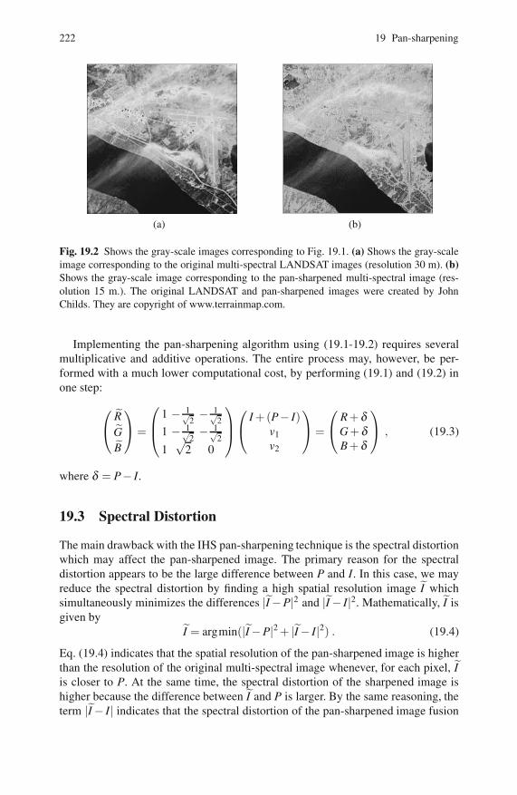
222 19 Pan-sharpening
(a) (b)
Fig. 19.2 Shows the gray-scale images corresponding to Fig. 19.1. (a) Shows the gray-scaleimage corresponding to the original multi-spectral LANDSAT images (resolution 30 m). (b)Shows the gray-scale image corresponding to the pan-sharpened multi-spectral image (res-olution 15 m.). The original LANDSAT and pan-sharpened images were created by JohnChilds. They are copyright of www.terrainmap.com.
Implementing the pan-sharpening algorithm using (19.1-19.2) requires severalmultiplicative and additive operations. The entire process may, however, be per-formed with a much lower computational cost, by performing (19.1) and (19.2) inone step:
⎛
⎝
˜R˜G˜B
⎞
⎠=
⎛
⎜
⎝
1 − 1√2− 1√
21 − 1√
2− 1√
21√
2 0
⎞
⎟
⎠
⎛
⎝
I +(P− I)v1
v2
⎞
⎠=
⎛
⎝
R + δG+ δB + δ
⎞
⎠ , (19.3)
where δ = P− I.
19.3 Spectral Distortion
The main drawback with the IHS pan-sharpening technique is the spectral distortionwhich may affect the pan-sharpened image. The primary reason for the spectraldistortion appears to be the large difference between P and I. In this case, we mayreduce the spectral distortion by finding a high spatial resolution image ˜I whichsimultaneously minimizes the differences |˜I−P|2 and |˜I− I|2. Mathematically, ˜I isgiven by
˜I = argmin(|˜I−P|2 + |˜I− I|2) . (19.4)
Eq. (19.4) indicates that the spatial resolution of the pan-sharpened image is higherthan the resolution of the original multi-spectral image whenever, for each pixel, ˜Iis closer to P. At the same time, the spectral distortion of the sharpened image ishigher because the difference between ˜I and P is larger. By the same reasoning, theterm |˜I− I| indicates that the spectral distortion of the pan-sharpened image fusion

19.3 Spectral Distortion 223
is lower whenever, for each pixel, ˜I is closer to I. At the same time, the spatialresolution of the sharpened image is lower than that of the sharpened image obtainedwith the traditional IHS method. We see, that depending on ˜I, we may establish atrade-off between the spatial and spectral resolution of the pan-sharpened image.This is the basis of the pan-sharpening algorithm developed by Choi [2].
19.3.1 Pan-sharpening Algorithm of Choi
Eq. (19.4) forms the basis of the pan-sharpening algorithm of Choi [2]. We considertwo special cases:
˜I = P. In this case the absolute difference |˜I− I| is maximal. As a consequence,the spectral distortion is maximal and the spatial resolution is high.
˜I = I. In this case the absolute difference |˜I− I| is zero. As a consequence, thespectral distortion is minimal (zero) and the spatial resolution is low.
Choi uses a parametric solution ˜I(t) which is linear between the two limiting cases:
˜I = P− P− It
, (19.5)
where t is a parameter and the limiting cases are recovered when t = ∞ and t = 1.Eqn. (19.5) implies that as t increases from 1 to∞, both the spatial resolution and thespectral distortion of ˜I will increase. In the Choi algorithm, we balance the spatialresolution with the spectral resolution using the parameter t, which is called thetrade-off parameter. The pan-sharpened image of Choi is:
⎛
⎝
˜R˜G˜B
⎞
⎠ =
⎛
⎝
R + δG+ δB + δ
⎞
⎠=
⎛
⎝
R +(P− I)(1−1/t)G+(P− I)(1−1/t)B +(P− I)(1−1/t)
⎞
⎠ , (19.6)
where δ = ˜I− I = (P− I)(1−1/t).The Choi method is fast and easy to implement. Moreover, according to the pur-
pose of each application, different user-specified tradeoff parameters can be usedfor user-specified multi-spectral images.
To evaluate the spectral distortion in (19.6) we compare (˜R ˜G˜B) with the multi-spectral image (RGB) after conversion into the IHS color space using (16.1-16.3):
˜I =13(˜R + ˜G+ ˜B) = I + δ ,
˜H = cos−1(
˜R− (˜G+ ˜B)/2√
(˜R− ˜G)2 +(˜R− ˜B)( ˜G− ˜B)
)
= H ,
˜S = 1− 3min(˜R, ˜G, ˜B)˜R+ ˜G+ ˜B
=IS˜I
.

224 19 Pan-sharpening
These equations demonstrate that while the hue of the pan-sharpened image is un-changed, the saturation is changed such that the product of the saturation and theintensity remains constant.
19.3.2 Pan-sharpening Algorithm of Tu et al.
Tu et al. [6] modified the pan-sharpening algorithm of Choi by multiplying the right-hand side of (19.6) by P/˜I. The pan-sharpening algorithm of Tu et al. is thus identi-cal to Choi apart from a simple energy normalization procedure. The correspondingTu pan-sharpened image is:
⎛
⎝
˜R˜G˜B
⎞
⎠ =P˜I
⎛
⎝
R + δG+ δB + δ
⎞
⎠=P˜I
⎛
⎝
R +(˜I− I)G+(˜I− I)B +(˜I− I)
⎞
⎠ ,
=P
P(1−1/t)+ I/t
⎛
⎝
R +(P− I)(1−1/t)G+(P− I)(1−1/t)B +(P− I)(1−1/t)
⎞
⎠ . (19.7)
To assess the spectral distortion of (19.7) we follow the same approach as beforeand obtain:
˜I =P˜I(I +˜I− I) = P ,
˜H = H ,
˜S = S .
These equations demonstrate that the hue and saturation of the pan-sharpened imageof Tue et al. are unchanged.
19.4 IKONOS
When IHS pan-sharpened methods are used with IKONOS imagery, there is a sig-nificant color distortion, due primarily to the range of wavelengths in an IKONOSpanochromatic image. Unlike the panochromatic images of SPOT and IRS sensors,IKONOS panochromatic images (as shown Fig. 2.5) have an extensive range ofwavelengths-from visible to near-infrared (NIR). This difference obviously inducesthe color distortion problem in IHS fusion as a result of the mismatches; that is, theP and I are spectrally dissimilar. In particular, the grey values of P in the green veg-etated regions are far larger than the grey values of I because the areas covered byvegetation are characterized by a relatively high reflectance of NIR and panochro-matic bands as well as a low reflectance in the R, G and B bands. To minimize theradiance differences between I and panchromatic P, we may include the NIR bandin the definition of the I component. A simple method for doing this is:

19.5 Wavelets 225
I =R +αG+βB + NIR
3, (19.8)
where 0≤ α ≤ 1 and 0≤ β ≤ 1 are two parameters and α+β = 1.IHS pan-sharpening is then extended from three color image (RGB) to the four
band image (RGB)+ NIR:
⎛
⎜
⎜
⎝
˜R˜G˜B˜NIR
⎞
⎟
⎟
⎠
=
⎛
⎜
⎜
⎝
R + δG+ δB + δ
NIR + δ
⎞
⎟
⎟
⎠
, (19.9)
where δ = P− I.Without loss of generality the pan-sharpening algorithm of Choi and Tu et al. may
be directly extended to (19.9). For example, the corresponding Tu et al. equationsare:
⎛
⎜
⎜
⎝
˜R˜G˜B˜NIR
⎞
⎟
⎟
⎠
=P
P(1−1/t)+ I/t
⎛
⎜
⎜
⎝
R +(P− I)(1−1/t)G+(P− I)(1−1/t)B +(P− I)(1−1/t)
NIR +(P− I)(1−1/t)
⎞
⎟
⎟
⎠
.
19.5 Wavelets
The basis of the IHS pan-sharpening technique is that the IHS transformation sepa-rates the spectral and spatial information of the multi-spectral RGB image. In prac-tice the separation of the spectral and spatial information is not complete: The Hand S components include some spatial information and the I component includessome spectral information. As a result IHS pan-sharpened images often differ signif-icantly from what the multi-spectral image would have if it had been collected at theresolution of the panchromatic image. One way to reduce the distortion is to retainthe I component while adding spatial details of the panchromatic image which aremissing from the multi-spectral image. This is the central idea of the IHS-waveletalgorithm.
The detail information of the PAN image that corresponds to structures of fea-tures with a size between the spatial resolution of the PAN image and that of theMS one is extracted using the multi-resolution wavelet decomposition in an undec-imated way.
Multi-resolution analysis allows us to decompose images into a sequence ofwavelet detail planes which correspond to structures of a given size.
The idea of wavelet-IHS pan-sharpening is instead of replacing the I componentwith the panchromatic image we simply add spatial details of the panchromatic im-age which are missing from the I component. The wavelet decomposition providesus with a simple way of doing this.

226 19 Pan-sharpening
The main steps in the method (assuming a spatial resolution ratio of 1 : 4) [4, 5]are as follows (see also Ex. 8.6):
1. Spatially align the multi-spectral image and the panchromatic image. Then re-sample the multi-spectral image to make its pixel size equal to that of thepanchromatic image.
2. Apply the IHS transform to the multi-spectral image and obtain the correspond-ing intensity, hue and saturation components I, H and S.
3. Generate a new panchromatic image P whose histogram matches that of the Iimage.
4. Decompose P using the undecimated wavelet decomposition. We obtain two
wavelet detail images y(P)1 and y(P)
2 and an approximation (residual) image P2.
Repeat for I. We obtain two wavelet detail images y(I)1 and y(I)
2 and an approxi-
mation (residual) image I2. By definition, the detail images y(P)1 and y(P)
2 pick upstructural details which are not present I.
5. Calculate the difference δ = ˜I− I =∑k y(P)k −∑k y(I)
k , where ∑k y(P)k = y(P)
1 + y(P)2
and ∑k y(I)k = y(I)
1 + y(I)2 .
6. Insert the spatial information of the panchromatic image into the multi-spectralimage through the inverse IHS transform.
Mathematically,
⎛
⎝
˜R˜G˜B
⎞
⎠ =
⎛
⎝
R +(˜I− I)G+(˜I− I)B +(˜I− I)
⎞
⎠ ,
=
⎛
⎜
⎝
R +(∑y(P)k −∑y(I)
k )G+(∑y(P)
k −∑y(I)k )
B +(∑y(P)k −∑y(I)
k )
⎞
⎟
⎠.
The new saturation value for the image fused by the method of Gonzlez-Audcanaet al. then becomes
˜S = 1− 3min(R + δ ,G+ δ ,B + δ )R + G+ B + 3δ
, (19.10)
where δ = ˜I− I and˜SS
=1˜I
=1
1 + δ. (19.11)
19.6 Sensor Spectral Response
If we calibrate the panchromatic image P and the three color images R, G, B inthe multi-spectral image, then we may introduce the spectral response φ(ν) of thesensors into (19.3) as follows [3, 7]: We calibrate P, R, G and B in terms of thecorresponding number of photons. Thus

References 227
P = nP , R = nR , G = nG and B = nB .
In this case, the number of photons corresponding to the intensity component I isnI:
nI = (nR + nG + nB)/3 .
Let I = nI denote the estimated intensity of the multi-spectral image if it works atthe spatial resolution of the panchromatic sensor. Then the proposed pan-sharpenedimage [3] is:
⎛
⎝
nR
nG
nB
⎞
⎠=
⎛
⎝
nR + δnR/nI
nG + δnG/nI
nB + δnB/nI
⎞
⎠ .
where δ = nI−nI and according to (2.2):
nI =nR + nG + nB
3,
=nP
3
(
∫
φR(ν)dν +∫
φG(ν)dν+∫
φB(ν)dν)/
∫
φP(ν)dν .
References
1. Alparone, L., Wald, L., Chanussot, J., Thomas, C., Gamba, P., Bruce, L.M.: Comparison ofpansharpening algorithms: outcome of the 2006 GRS-S data fusion contest. IEEE Trans.Geosci. Remote Sensing 45, 3012–3021 (2007)
2. Choi, M.: A new intensity-hue-saturation approach to image fusion with a tradeoff param-eter. IEEE Trans. Geosci. Remote Sens. 44, 1672–1682 (2006)
3. Gonzalez-Audicana, M., Otazu, X., Fors, O., Alvarez-Mozos, J.: A low computational-cost method to fuse IKONOS images using the spectral response function of its sensors.IEEE Trans. Geosci. Remote Sens. 44, 1683–1691 (2006)
4. Gonzalez-Audicana, M., Otazu, X., Fors, O., Seco, A.: Comparison between Mallat’s andthe ’a trous’ discrete wavelet transform based algorithms for the fusion of multispectraland panchromatic images. Int. J. Remote Sens. 26, 595–614 (2005)
5. Gonzalez-Audicana, M., Saleta, J.L., Catalan, R.G., Garcia, R.: Fusion of multispectraland panchromatic images using improved IHS and PCA mergers based on wavelet de-composition. IEEE Trans. Geosci. Remote Sens. 42, 1291–1299 (2004)
6. Tu, T.-M., Cheng, W.-C., Chang, C.-P., Huang, P.S., Chang, J.-C.: Best tradeoff for high-resolution image fusion to preserve spatial details and minimize color distortion. IEEEGeosci. Remote Sens. Lett. 4, 302–306 (2007)
7. Otazu, X., Gonzalez-Audicana, M., Fors, O., Nunez, J.: Introduction of sensor spectralresponse into image fusion methods. Application to wavelet-basedmethods. IEEE Trans.Geosci. Remote Sens. 43, 2376–2385 (2005)

Chapter 20Ensemble Color Image Segmentation
Abstract. The subject of this chapter is ensemble color image segmentation. This isan image fusion application in which combine several simple image segmentationalgorithms to obtain a state-of-the-art image segmentation algorithm. The goal ofimage segmentation is to decompose the input image into a set of meaningful orspatially coherent regions sharing similar attributes. The algorithm is often a crucialstep in many video and computer vision applications such as object localizationor recognition. A simple image segmentation is the K-means cluster algorithm inwhich we divide the pixels into K clusters.
20.1 Introduction
The goal of image segmentation is to decompose the input image into a set of mean-ingful or spatially coherent regions sharing similar attributes. The algorithm is oftena crucial step in many video and computer vision applications such as object local-ization or recognition.
Present-day state-of-the-art segmentation algorithms obtain a high performanceby becoming more and more complex. In this chapter we describe a different ap-proach in which a high quality segmentation is obtained by fusing together a largeensemble of simple image segmentation algorithms [1].
The new algorithm works as follows:
Ensemble. Given an input image I∗ we create an ensemble of K images Ik,k ∈{1,2, . . . ,K}, by transforming I∗ into K different color spaces.
K-means Segmentation. Each image Ik is segmented into a L label decision im-age Dk using the K-means cluster algorithm, although any simple segmentationalgorithm may be used instead.
K-means Fusion. Form a high quality segmented image ˜D by fusing together theDk,k ∈ {1,2, . . . ,K}:
˜D = f (D1,D2, . . . ,DK) ,

230 20 Ensemble Color Image Segmentation
where f is an appropriate fusion operator. In [1] the K-means cluster algorithmis also used as the fusion operator.
We now consider in more detail each of these steps.
20.2 Image Ensemble
Given an input image I∗ in RGB space we create a ensemble of K images Ik,k ∈{1,2, . . . ,K}, by transforming I∗ into K different color spaces Sk. Each color spaceemphasizes a different property. The color spaces used by Mignotte are:
RGB. This tri-chromatic space is non-linear with regard to visual perception.HSV. This space decouples the chromatic information from shading effects.YIQ. This space takes into account the human color charcateristics.XYZ. This is a pscho-visually linear space.LAB. This space approximates the human vision system. Its L component closely
matches the human perception of lightness.LUV. This a Euclidean space which yields a perceptually uniform spacing of
color.
20.3 K-Means Segmentation
We segment each image Ik using the K-means cluster algorithm (see Ex. 6.8). In theconventional K-means we assign each pixel m,m ∈ {1,2, . . . ,M}, to a given cluster
C(k)l :
δ (k)l (m) =
{
1 if c(k)m is assigned to C(k)
l ,0 otherwise .
where c(k)m is the representation of the mth pixel in Ik, i. e. in the color space Sk. The
assignments δ (k)l (m) define the corresponding segmented image Dk:
Dk(m) = l if δ (k)l (m) = 1 .
The K-means algorithm attempts to find the set of cluster centers Cl such that theoverall error
E(k) =∑m
L
∑l=1
δ (k)l (m)d(cm,C(k)
l )
is a minimum, where d(c(k)m ,C(k)
l ) is an appropriate distance (similarity) measure
between c(k)m and C(k)
l .The cluster centers are found in an iterative procedure. In each iteration we calcu-
late the assignment δ (k)l (m) using the cluster centers C(k)
l calculated in the previousiteration. The cluster centers are then recalculated using the new assignment:

20.4 K-Means Fusion Operator 231
for m = 1 : M
δ (k)h (m) =
{
1 if d(c(k)m ,C(k)
h ) = minl d(c(k)m ,C(k)
l )0 otherwise;
endfor l = 1 : L
c(k)m = ∑M
m=1 δ(k)l (m)c(k)
m /∑Mm=1 δ
(k)l (m);
end
For an image I(k) in RGB space, the color components (rm,gm,bm) for each pixelm,m ∈ {1,2, . . . ,M}, are all measured on the same linear scale. In this case, anappropriate similarity (distance) measure is the Euclidean distance:
d(c(k)m ,C(k)
l ) =√
(r(k)m −R(k)
l )2 +(g(k)m −G(k)
l )2 +(b(k)m −B(k)
l )2 .
However, the Euclidean distance is not appropriate for the other color spaces, HSV,YIQ, XYZ, LAB and LUV, where the color components (hm,sm,vm), (ym, im,qm),(xm,ym,zm), (lm,am,bm) and (lm,um,vm) are not measured on the same linear scale.
At first sight it may be though very difficult to find a universal similarity(distance) measure. However, Mignotte [1] shows we may define such a similaritymeasure by converting the color components of each pixel into a local probabilitydistribution.
Let p(k)m be the local distribution of the pixel values in a window centered on the
mth pixel in I(k). If P(k)l denotes the average distribution of pixel values which are
assigned to the l cluster,
P(k)l =
M
∑m=1
δ (k)l (m)p(k)
m /M
∑m=1
δ (k)l (m) ,
then Mignotte defines d(c(k)m ,C(k)
l ) as
d(c(k)m ,C(k)
l ) = S(p(k)m , P(k)
l ) ,
where S is the Bhattacharyya similarity (distance) measure.
Given the Mignotte distance measure d(c(k)m ,C(k)
l ), we may cluster the pixels us-ing the K-means cluster algorithm.
20.4 K-Means Fusion Operator
Mignotte also uses the K-means cluster algorithm as a fusion operator as fol-
lows. Given the segmented images D(k),k ∈ {1,2, . . . ,K}, let q(k)m denote the local

232 20 Ensemble Color Image Segmentation
distribution of segmentation labels in a window centered on the mth pixel in D(k).
We now concatenate the distributions q(k)m :
qm ≡ (q(1)m ,q(2)
m , . . . ,q(K)m ) .
The concatenated distributions qm may then be clustered into LQ clusters using the
K-means algorithm in the same way we clustered the p(k)m . The result is an assign-
ment matrix:˜δl(m) =
{
1 if qm is assigned to ˜Cl ,0 otherwise .
The assignment matrix ˜δl(m) then defines the fused segmentation image ˜D:
˜D(m) = l if ˜δl(m) = 1 .
Reference
1. Mignotte, M.: Segmentation by fusion of histogram-based K-means clusters in differentcolor spaces. IEEE Trans. Image Process. 17, 780–787 (2008)

Chapter 21STAPLE: Simultaneous Truth and PerformanceLevel Estimation
Abstract. The subject of this chapter is the STAPLE (Simultaneous Truth and Per-formance Level Estimation) algorithm. This is a method for fusing together severalsegmented images and is based on the expectation-maximization (EM) algorithm.
21.1 Introduction
Segmentation by non-rigid registration to an atlas image is an established methodfor labeling biomedical images [1]. However, in general, the choice of atlas imageis important in determining the quality of the segmentation. As a result, multiple at-lases are often used which may improve the segmentation accuracy over approachesthat use a single individual atlas or even an average atlas (see Sect. 10.8). These algo-rithms often combine the multiple segmentations by a majority-vote rule. However,[2, 3] have shown that much better results may be produced by using the STAPLE(Simultaneous Truth and Performance Level Estimation) procedure . The STAPLEprocedure uses the expectation-maximization (EM) algorithm to iteratively estimatethe quality of the individual segmentations. The final segmentation is then computedwith these individual segmentation qualities taken into account by weighting the de-cisions made by a reliable segmentation algorithm higher than ones made by a lessreliable algorithm.
21.2 Expectation-Maximization Algorithm
The expectation-maximization (EM) is a powerful iterative technique suited for cal-culating the maximum likelihood estimate in problems where the observation can beviewed as incomplete data. The maximum-likelihood estimate of a random variablex, denoted as x, based on the incomplete observed data y, is defined as
x = argmaxx
(log p(y|x)) ,
where log p(y|x) is the log likelihood of y given x.

234 21 STAPLE: Simultaneous Truth and Performance Level Estimation
Central to the EM algorithm is the introduction of an auxiliary random variableW with log likelihood log p(W |x). The data W is referred to as the complete databecause it is more informative than y. The complete data W is not observed directly,but indirectly through y via the relationship y = f (W ), where f is a many-to-onemapping function. Those unobserved variables are referred to as hidden data anddenoted by H. The EM algorithm calculates an estimate for x, x, through an iterativeprocedure in which the next iteration’s estimate of x is chosen to maximize theexpectation of log p(W |x) given the incomplete data y and the current iteration’sestimate of x. For a review of the EM algorithm when we use a mixture of Gaussiansfor the likelihood see Sect. 7.3.
21.3 STAPLE
Given a medical input image I, our task is to estimate its ground truth segmen-tation vector T . Writing I as a one-dimensional vector with M pixels I(m),m ∈{1,2, . . . ,M}, then
T (m) ={
1 if a given structure exists at mth pixel ,0 otherwise .
Suppose we have segmented I using K different experts and/or algorithms. LetBk,k ∈ {1,2, . . . ,K}, denote the corresponding segmentation vectors. Then our aimis to create a vector ˜B by combining the individual Bk such that ˜B is a good approx-imation to the (unknown) ground truth segmentation vector T .
We have already considered this problem in Chapts. 7 and 12. Here we show howwe may use the expectation-maximization (EM) algorithm to form ˜Bk.
Different experts and/or segmentation algorithms will have different segmenta-tion qualities. We represent the quality of each expert, or segmentation, algorithmwith a 2×2 matrix λk, where λk(r,s) is the conditional probability that the true clas-sification of the mth pixel is T (m) = r,m ∈ {1,2, . . . ,M}, while the kth expert, oralgorithm, predicts Bk(m) = s. The diagonal entries (λk(r,s) represent the likelihoodof correct classification. The sum ∑r λk(r,r) is referred to as the sensitivity of thekth algorithm:
sensitivity = λk(0,0)+λk(1,1) .
The off-diagonal entries (λk(r,s),r �= s) represent the likelihood of incorrect classi-fication of the kth expert. The sum ∑r �=s λk(r,s) is referred to as the specificity of thekth algorithm:
specificity = λk(1,0)+λk(0,1) .
In the STAPLE algorithm we generate ˜B and estimate the matrices λk,k ∈ {1,2, . . . ,K}, using an iterative EM algorithm. In the E-step of the algorithm weestimate the a posteriori probability of the ground true segmentation T . Then in the
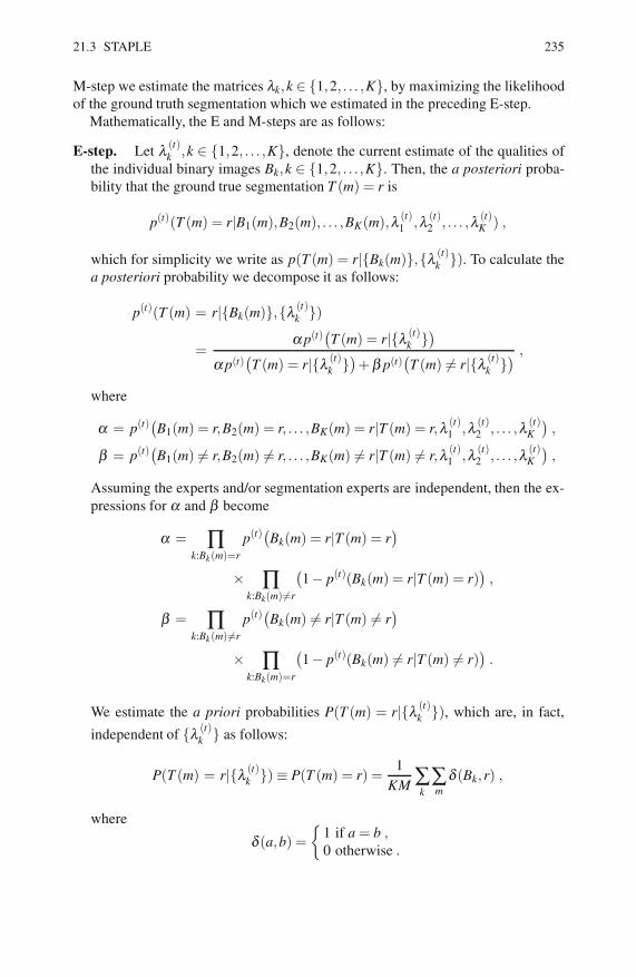
21.3 STAPLE 235
M-step we estimate the matrices λk,k ∈ {1,2, . . . ,K}, by maximizing the likelihoodof the ground truth segmentation which we estimated in the preceding E-step.
Mathematically, the E and M-steps are as follows:
E-step. Let λ (t)k ,k ∈ {1,2, . . . ,K}, denote the current estimate of the qualities of
the individual binary images Bk,k ∈ {1,2, . . . ,K}. Then, the a posteriori proba-bility that the ground true segmentation T (m) = r is
p(t)(T (m) = r|B1(m),B2(m), . . . ,BK(m),λ (t)1 ,λ (t)
2 , . . . ,λ (t)K ) ,
which for simplicity we write as p(T (m) = r|{Bk(m)},{λ (t)k }). To calculate the
a posteriori probability we decompose it as follows:
p(t)(T (m) = r|{Bk(m)},{λ (t)k })
=α p(t)(T (m) = r|{λ (t)
k })
α p(t)(
T (m) = r|{λ (t)k }
)
+β p(t)(
T (m) �= r|{λ (t)k }
)
,
where
α = p(t)(B1(m) = r,B2(m) = r, . . . ,BK(m) = r|T (m) = r,λ (t)1 ,λ (t)
2 , . . . ,λ (t)K
)
,
β = p(t)(B1(m) �= r,B2(m) �= r, . . . ,BK(m) �= r|T (m) �= r,λ (t)1 ,λ (t)
2 , . . . ,λ (t)K
)
,
Assuming the experts and/or segmentation experts are independent, then the ex-pressions for α and β become
α = ∏k:Bk(m)=r
p(t)(Bk(m) = r|T (m) = r)
× ∏k:Bk(m) �=r
(
1− p(t)(Bk(m) = r|T (m) = r))
,
β = ∏k:Bk(m) �=r
p(t)(Bk(m) �= r|T (m) �= r)
× ∏k:Bk(m)=r
(
1− p(t)(Bk(m) �= r|T (m) �= r))
.
We estimate the a priori probabilities P(T (m) = r|{λ (t)k }), which are, in fact,
independent of {λ (t)k } as follows:
P(T (m) = r|{λ (t)k })≡ P(T (m) = r) =
1KM∑k ∑m
δ (Bk,r) ,
where
δ (a,b) ={
1 if a = b ,0 otherwise .

236 21 STAPLE: Simultaneous Truth and Performance Level Estimation
M-step. We update the parameters λ (t)k ,k ∈ {1,2, . . . ,K}, by maximizing the like-
lihood of the current ground truth estimate determined in the E-step. Given the
previous ground truth estimates p(t)(
T (m) = r|Bk(m),λ (t)k
)
, the new estimatesfor the expert parameters are:
λ (t+1)k (r,r) =
∑m:Bk(m)=r p(t)(T (m) = r|{Bk(m)},{λ (t)k }
)
∑m p(t)(
T (m) = r|{Bk(m)},{λ (t)k }
)
,
λ (t+1)k (r,s) =
∑m:Bk(m) �=r
(
1− p(t)(T (m) = r|{Bk(m)},{λ (t)k })
)
∑m
(
1− p(t)(T (m) = r|{Bk(m)},{λ (t)k })
)
,
where s �= r. After several iterations the a posteriori probabilities p(t)(T (m) =r|{Bk(m)},{λ (t)
k }) and the parameters λ (t)k ,k ∈ {1,2, . . . ,K}, converge to their fi-
nal values. The ˜B(m) are then assigned to the class with the maximum a posterioriprobability:
˜B(m) ={
1 if p(T (m) = 1|{Bk},{λk})≥ 0.5 ,0 otherwise .
.
References
1. Dawant, B.M., Hartmann, S.L., Thirion, J.P., Maes, F., Vandermeulen, D., Demaerel, P.:Automatic 3-D segmentation of internal structures of the head in MR images usning acombination of similarity and free-form transformations: part I, methodology and valida-tion on normal subjects. IEEE Trans. Med. Imag. 18, 909–916 (1999)
2. Rohlfing, T., Russakoff, D.B., Muurer Jr., C.R.: Performance-based classifier combinationin atlas-based image segmentation using expectation-maximization parameter estimation.IEEE Trans. Med. Imag. 23, 983–994 (2004)
3. Warfield, S.K., Zou, K.H., Wells, W.M.: Simultaneous truth and performance level esti-mation (STAPLE): An algorithm for the validation of image segmentation. IEEE Trans.Med. Imag. 23, 903–921 (2004)

Chapter 22Biometric Technologies
Abstract. In this chapter we provide a brief overview of biometric technology andin particular, multi-modal biometric technology.
22.1 Introduction
We define biometric technology to be the automated use of physiological, or behav-ioral, characteristics to determine, or verify, an individual’s identity. We shall followcommon practice and use the word biometric to refer to any human physiological,or behavioral, characteristic which possesses the following properties:
Universal. Every person should have the biometric characteristic.Unique. No two people should be exactly the same in terms of the biometric
characteristic.Permanent. The characteristic should be invariant with time.Collectable. The characteristic can be measured quantitatively.Reliable. The characteristic must be safe and operate at a satisfactory perfor-
mance level.Acceptable. The characteristic should be non-invasive and socially tolerable.Non-circumventable. The system should be robust against impostors.
Biometric characteristics include visual images and other human phenomena suchas speech, gait, odour and DNA.
Example 22.1. Biometric Recognition Systems [4]. A typical use of biometricrecognition systems is in access control. In this case, we have a person claim-ing an identity and provides a biometric sample to support this claim. Thebiometric recognition system acting as an authentication system then classi-fies the person as either a true claimant or as an imposter.
In fact biometric recognition systems can be used in three distinct ways [4].

238 22 Biometric Technologies
Closed set identity. Classifying a given biometric sample as belonging toone of K persons, where K is the number of known persons.
Open set identity. Assigning a given biometric sample to one of K + 1classes, where the first K classes represent the K persons in the closed setidentity and class K + 1 represents an “unknown” or “previously unseen”person.
Authentication. Assign a given sample into one of two classes: either thesample belongs to a specific person or it does not.
22.2 Multi-modal Biometrics
Although there has been a significant improvement in the performance of single-sensor biometric systems, real-life environments still pose significant difficulties onbiometric-based recognition systems.
Example 22.2. Unconstrained Iris Recognition [7, 9]. Iris recognition authen-ticates and recognizes persons using the unique iris pattern. When the irisimage is taken in a controlled environment, the accuracy of the system is veryhigh. However in uncontrolled environments the performance of the systemdegrades considerably due to noise factors such as eyelids, eyelashes and re-flection.
To increase overall reliability, the contemporary biometric systems often employmultiple physiological, or behavioral, traits. This approach is called multi-modalbiometrics.
The most often multi-biometric data, employed in the biometric systems, includeiris and retina of the eye, fingerprint, geometry and palmprint of the hand, and alsoface and ears. We often combine complimentary biometric sensors. For example,face geometry is a highly dynamic but rich topological structure (smile, lip, brow,and eye movements). Combining facial images with more static biometric such asfingerprint, is an example of the concept of multi-biometrics.
The multi-modal human recognition is deployed in physical access security sys-tems and other areas such as banking systems [11].
22.2.1 Fingerprints
Fingerprint is, perhaps, the oldest type of biometrics and today the fingerprint readeris the most developed type of biometric sensors.

22.3 Multi-biometrics 239
22.2.2 Signatures
Current interest in signature analysis is motivated by the development of improveddevices for human-computer interaction which enable input of handwriting and sig-natures.
22.2.3 Faces
Face recognition systems detect patterns, shapes, and shadows in the face, performfeature extraction and recognition of facial identity. Today, the most popular ap-proach is based on principal component analysis (see Chapt. 9).
However many face recognition systems are confused when identifying the sameperson smiling, aged, with various accessories (moustache, glasses), and/or in badlylit conditions. For a comprehensive review of the current approaches to face recog-nition see [12].
22.2.4 Iris and Retina
Iris recognition systems scan the surface of the iris to compare patterns. The irisbiometrics [2] is considered to be the most reliable one. Retina recognition systemsscan the surface of the retina and compare nerve patterns, blood vessels and suchfeatures [5].
22.2.5 Gait Biometrics
Gait recognition is defined as the identification of a person through the pattern pro-duced by walking [3]. A unique advantage of using gait as a biometric is that itoffers the potential for recognition at a distance or at low resolution, when otherbiometrics might not be perceivable. However, this must be balanced with the largewithin-subject variation exhibited by a gait biometric [3].
22.2.6 Other Biometrics
A variety of biometrics such as ear geometry [6], odour, electrocardiogram andkeystroke dynamics [11].
22.3 Multi-biometrics
Apart from multi-modal systems, multi-biometrics include multi-sensor, multi-algorithm, multi-instance and multi-sample systems [10, 11].

240 22 Biometric Technologies
22.3.1 Multi-sensor System
Multi-sensor systems employ multiple sensors to capture a single biometric trait.The following example illustrates multi-sensor face recognition which is performedby fusing thermal infra-red and visible light face images together.
Example 22.3. Face Recognition by Fusing Thermal Infrared and VisibleImaqery [1]. Thermal infrared (IR) imagery offers a promising alternative tovisible, or electro-optical (EO), imagery for face recognition due to its rela-tive insensitivity to changes in illumination. However thermal IR is opaque toglass. This means part of the face may be occluded if the person is wearingeyeglasses.
The IR and EO images are fused together in the wavelet domain (Chapt. 8).In [1] a genetic algorithm is used to find the optimum strategy to combine theinformation from the two spectra (cf. Ex. 8.4). The objective is to compute afused image which captures the most salient features from the inputs.
Face recognition is then performed using a conventional principal compo-nent analysis of the fused image. The results showed a significant improve-ment in recognition.
22.3.2 Multi-algorithm System
Multi-algorithm systems use multiple feature extraction and/or matching algorithmson the same biometric data. The idea underlying a multi-algorithm system is thatdifferent features and/or matching algorithm emphasize different aspects of the testobject. Their combination may therefore give an improved biometric performance.The following example illustrates a multi-algorithm face recognition system whichis performed by fusing PCA (principal component analysis) and LDA (linear dis-criminant analysis) algorithms.
Example 22.4. Decision-level Fusion of PCA and LDA-based Face Recogni-tion Algorithms [8]. Face recognition is often performed using principal com-ponent analysis (PCA) (Sect. 9.2) or linear discriminant analysis (LDA) (Sect9.5). In [8] face recognition is performed by fusing together the outputs of aPCA and a LDA face recognition algorithm.
Let x denote a given test image written as a one-dimensional vector. Weproject x onto the PCA and LDA sub-spaces. Let u and v be the correspondingprojected vectors. If Uk and Vk are, respectively, the kth training pattern inthe PCA and LDA sub-spaces, then we compute the corresponding Euclidean

22.4 Epilogue 241
distances dPCAk = ‖u−Uk‖ and dLDA
k = ‖v−Vk‖. The Euclidean distance arenormalized and are then combined together to a given fused distance ˜Dk:
˜Dk =DPCA
k + DLDAk
2.
where
DPCAk =
dPCAk −minl(d
(PCAl )
maxl(dPCAl )−minl(dPCA
l ),
DLDAk =
dLDAk −minl(d
(LDAl )
maxl(dLDAl )−minl(dLDA
l ).
The fused distances ˜Dk are then used in a nearest neighbor classifier instead ofdPCA
k or dLDAk . The results obtained with ˜Dk show a significant improvement in
performance.
22.3.3 Multi-instance System
Multi-instance systems use multiple instances of the same biometric. For example,we may use the fingerprints from the left and right index fingers, or irises from theleft and right eye, to verify an individual.
22.3.4 Multi-sample System
Multi-sample systems use multiple samples of the same biometric trait obtainedwith the same sensor. For example a fingerprint system equipped with a small sizesensor may acquire multiple dab prints of an individual’s finger in order to obtain acomplete fingerprint image.
22.4 Epilogue
The aim of the book has been to provide a practical introduction to the theories,techniques and applications of image fusion. In Part I we considered the conceptualtheories and ideas which underlie image fusion and in Part II we considered some ofthe techniques and algorithms which are used in image fusion. In Part III we consid-ered four real-life applications of image fusion. Apart from these four applications,numerous examples of image fusion are given in Parts I and II. The reader is nowencouraged to review these examples.

242 22 Biometric Technologies
References
1. Bebis, G., Gyaourova, A., Singh, S., Pavlidis, I.: Face recognition by fusing thermalinfrared and visible imagery. Image Vis. Comp. 24, 727–742 (2006)
2. Bowyer, K.W., Hollingsworth, K., Flynn, P.S.: Image understanding for iris biometrics:a survey. Comp. Vis. Image Understand. 11, 281–307 (2008)
3. Boulgouris, N.V., Hatzinakos, D., Plataniotis, K.N.: Gait recognition: a challenging sig-nal processing technology for biometric identification. IEEE Sig. Process. Mag. (Novem-ber 2005)
4. Cardinaux, F., Sanderson, C., Bengio, S.: User authentication via adapted statistical mod-els of face images. IEEE Trans. Sig. Process. 54, 361–373 (2005)
5. Daugman, J.: The importance of being random: statistical principles of iris recognition.Patt. Recogn. 36, 279–291 (2003)
6. Hurley, D.J., Nixon, M.S., Carter, J.N.: Force field feature extraction for ear biometrics.Comp. Vis. Image Understand. 98, 491–512 (2005)
7. A robust eyelash detection based on iris focus assessment. Patt. Recogn. 28, 1630–1639(2007)
8. Marcialis, G.L., Roli, F.: Decision-level fusion of PCA and LDA-based face recognitionalgorithms. Int. J. Image Graphics 6, 293–311 (2006)
9. Min, T.-H., Park, R.-H.: Comparison of eyelid and eyelash detection algorithms for per-formance improvement of iris recognition. In: Proc. Int Conf. Image Proc. (2008)
10. Ross, A.: An introduction to multibiometrics. In: Proc. 15th Eur. Sig. Proc. Conf. (2007)11. Ross, A., Nandakumar, K., Jain, A.K.: Handbook of multibiometrics. Springer, Heidel-
berg (2006)12. Zhao, W., Chelappa, R. (eds.): Face Processing: Advanced Modeling and Methods. El-
sevier, Amsterdam (2006)

Index
AGCsee Automatic gain control, 187
Assignment problemHungarian algorithm, 58semantic equivalence, 57
Atlas-based segmentation 139Automatic gain control 187
comparametric function, 190radiometric response function, 189
Baggingbootstrapping, 144clustering, 145nearest neighbor classifier, 145pattern recognition, 144
Bayer filter 11Boosting 147
adaboost, 147, 148ave2boost, 148object detection, 152pattern recognition, 147Viola-Jones, 151
Bootstrapping 31, 143Brain atlas
common representational format, 21Brovey pan-sharpening 80
Canonical correlation analysis (CCA)121
CCAsee Canonical correlation analysis,
121Change detection
expectation-maximization, 77
Circular statistics 201Classification
bagged nearest neighbor, 145ensemble nearest neighbor, 140inner distance, 27nearest neighbor, 140object recognition, 25photometric color invariants, 27shape context, 25
Clustering 145K-means algorithm, 70, 202, 230bagging, 145color image segmentation, 230mean shift algorithm, 132periodic attributes, 202
Co-association matrixsemantic equivalence, 60
Color spaces 196HLS, 198HSV, 198IHLS, 198IHS, 197indirect IHS, 200multiple, 202perceptual model, 197photometric color invariants, 27
Common representational format 23“Bull’s-eye”image(s), 24bootstrapping, 31brain atlas, 21geographical information system, 23inner distance, 27local binary pattern, 28mosaic image, 23, 41

244 Index
radiometric calibration, 22semantic equivalence, 22, 53shape context, 25spatial alignment, 22, 41thresholding, 155
Decision fusion 83expectation-maximization, 236majority-vote rule, 83shape-based averaging, 84STAPLE, 233
Digital camera 9Bayer filter, 11, 12CCD camera, 13noise, 11optical system, 9orthographic projection, 10perspective projection, 10quantization, 12recording system, 10spatial resolution, 14spatial sampling, 11spectral resolution, 15
Discrete wavelet transform 94a trous, 96dual-tree complex wavelet transform,
96edge detection, 98fusion, 98spot detection, 98undecimated, 96
Distance transform 85shape-based averaging, 85signed, 85
Dual-tree complex wavelet transform96
DWTsee Discrete wavelet transform, 94
Earth mover’s distancecircular EMD, 174Mallow’s distance, 175non-negative matrix factorization,
116Edge detection
discrete wavelet transform, 98EM algorithm
see Expectation-maximization, 236Ensemble learning
adaboost, 147ave2boost, 148bagging, 144boosting, 147bootstrapping, 31, 143color image segmentation, 229ensemble atlas-based segmentation,
139face recognition, 135image transformations, 128multiple color spaces, 131multiple normalizations, 130multiple random convolutions, 129multiple segmentations, 132multiple sub-space transformations,
129multiple thresholds, 131, 135re-sampling methods, 143spatial sampling, 137white balance, 192
Expectation-maximization 233, 234change detection, 77decision fusion, 236discrete wavelet transform, 100Gaussian mixture model, 77generalized Gaussian mixture, 77STAPLE, 234
Face recognition 87, 112ensemble learning, 135local binary pattern, 87
Feature mapfusion, 81semantic equivalence, 81
Feature mapsradiometric calibration, 71
Fisher criterionlinear discriminant analysis, 117
Gaussian mixture model 100expectation-maximization, 77
Generalized Gaussian distribution77, 103
Geographical information systemcommon representational format, 23
Histogramoptimal bin number and width, 45,
175Sturges’ rule, 45

Index 245
Histogram calibrationsemantic equivalence, 56
Histogram matching 64Histogram specification 65Hungarian algorithm
assignment problem, 58
Image compositing 22Image fusion
addition, 76benefits, 1change detection, 77decision fusion, 83discrete wavelet transform, 98division, 80electro-optical and infra-red, 100expectation-maximization, 100, 236feature map fusion, 81Markov random field, 206mosaic image, 41multiplication, 80pixel operations, 75principal component analysis, 114processing chain, 2rank fusion, 81requirements, 6shadow detection, 80subtraction, 77synergy, 1
Image normalizationsee Radiometric calibration, 63
Image registrationsee Spatial alignment, 35
Image segmentationatlas-based, 139color, 229ensemble learning, 229, 230mean-shift algorithm, 132radiometric calibration, 70skin classification, 202
Image sensorsee Digital camera, 9
Image similaritysee Similarity measures, 167
Image stitching 22Image thresholding
categories, 155entropy, 159global, 155
histogram modification, 156Kittler-Illingworth, 158local, 137moments, 159Otsu, 158Ridler-Calvard, 158
Inner distance 27Iris recognition 238Isotonic calibration
semantic equivalence, 56
Key-pointdual-tree complex wavelet transform,
96, 165PCA-SIFT, 165SIFT, 163SURF, 165
LDAsee Linear discriminant analysis, 117
Linear discriminant analysis 117Fisher criterion, 117
Local binary pattern 28, 69face recognition, 87uniform, 29
Majority-vote ruledecision fusion, 83unsupervised weighted rule, 160
Markov random field 205, 206binary images, 206energy function, 207neighborhood structure, 205
Midway image equalization 66Moran’s autocorrelation coefficient
see Spatial alignment, 41Mosaic image 23
common representational format, 41compositing, 22stitching, 22
MRFsee Markov random field, 205
Multi-resolution analysisdiscrete wavelet transform, 94dual-tree complex wavelet transform,
96Mutual information
calculation, 45definition, 44histogram, 45

246 Index
interpolation effects, 48iso-intensity lines, 46partial volume interpolation, 47Parzen windows, 46small size effects, 49spatial alignment, 43spatial alignment artifacts, 48
Myocardial image(s)“Bull’s-eye image(s), 24
Nearest neighborbagged classification, 145classification, 140discriminant analysis, 120ensemble classification, 140
NMFsee Non-negative matrix factoriza-
tion, 115NNDA
see Nearest neighbor discriminantanalysis, 120
Non-negative matrix factorization115
earth mover’s distance, 116
Object detectionboosting, 152integral image, 151Viola Jones, 151
Object recognitionphotometric color invariants, 27
Pan-sharpening 219Brovey, 80Choi algorithm, 223discrete wavelet transform, 104IHS transformation, 220IKONOS images, 224principal component analysis, 114spectral distortion, 222
PAVsee Pooled-average value, 56
PCAsee Principal component analysis,
109Platt calibration
semantic equivalence, 55Pooled-average value 56Principal component analysis 109
2D-PCA, 113
face recognition, 112image fusion, 114pan-sharpening, 114Turk-Pentland trick, 110whitening, 112
PVIsee Partial volume interpolation, 47
Radiometric calibration 63features maps, 71histogram matching, 64histogram specification, 65image segmentation, 70local binary pattern, 69matching second-order statistics, 68midway image equalization, 66thresholding, 69
Re-sampling methodsadaboost, 147ave2boost, 148bagging, 144boosting, 147bootstrapping, 143ensemble learning, 143
Segmentationsee Image segmentation, 132
Semantic equivalenceassignment matrix, 57co-association matrix, 60definition, 53histogram calibration, 56isotonic calibration, 56permuting decision labels, 87Platt calibration, 55probabilistic scale, 54
Shadow detection 80Shape-based averaging 84Shape context
common representational format, 25SIFT
see Key-point, 25, 163Similarity measures 167
χ2, 172Bhat-Nayar, 180binary, 182cross-bin, 174cross-correlation coefficient, 177earth mover’s distance, 174

Index 247
global, 168Hausdorff, 183histogram bin selection, 175Kemeny-Snell, 179Kendall’s τ , 178local, 168Mallow’s distance, 175mean absolute error, 176mean square error, 176metric, 168Mittal-Ramesh, 182mutual information, 178order statistics, 178probabilistic, 170probability binning, 173Spearman’s ρ, 178
Skin classifier 202Spatial alignment 35
artifacts, 48hierarchical registration, 39image transformations, 37interpolation, 36Moran’s autocorrelation coefficient,
41mosaic image, 41multiple image constraints, 42mutual information, 43pairwise transformation, 36stitching, 43thin-plate splines, 37
Spectral resolution 15
Spot detectiondiscrete wavelet transform, 98
STAPLE algorithm 233, 234Stitching 43
feathering, 43Sturges’ rule
histogram bin calculation, 45Sub-space
face space, 107see CCA, ICA, LDA, NNDA, PCA,
107SURF
see Key-point, 165Surveillance systems 22
Texturelocal binary pattern, 28
Thresholdingensemble thresholding, 135fuzzy, 69radiometric calibration, 69
Vignetting 187causes, 188correction, 188
Viola-Jonesobject detection, 151
White balance 187adaptive algorithm, 192ensemble learning, 192
Whitening 112


