Impact of foundation modelling in o shore wind turbines ...

Impact of foundation modelling in offshore wind turbines: comparisonbetween simulations and field data

Ana M. Pagea,b, Veronika Næssa, Jacobus B. De Vaalc, Gudmund R. Eiksunda, Tor Anders Nygaardc

aNorwegian University of Science and Technology (NTNU), Trondheim, NorwaybNorwegian Geotechnical Institute (NGI), Oslo, NorwaycInstitute for Energy Technology (IFE), Kjeller, Norway

Abstract

The design of Offshore Wind Turbines (OWTs) relies on integrated simulation tools capable of predicting

the system dynamic characteristics and the coupled loads and responses. Despite all efforts to develop

accurate integrated models, these often fail to reproduce the measured natural frequencies, partly due

to the modelling of the foundation. Several foundation models and calibration approaches have been

proposed and compared with small or large scale field tests, where only the soil and the foundation

are included. However, there is a lack of more integral validation where the interaction between the

foundation and the structure is taken into account. The paper investigates the impact of the foundation

model and calibration approach on the simulated response of a monopile-based OWT installed in the

North Sea by comparing simulations and full-scale field data. The OWT structure and the environmental

actions are implemented in the aero-servo-hydro-elastic code 3DFloat. Two foundation models and two

calibration approaches are evaluated. The results indicate that, with a conceptually correct foundation

model and a realistic calibration, it is possible to match the measured natural frequency and predict

accurate fatigue loads. More accurate predicted loads will reduce uncertainties in the estimated fatigue

lifetime and therefore reduce risk in the design.

Keywords: Offshore Wind Turbine, Offshore measurement, Foundation Damping, Soil-Structure

Interaction, Load Calculation Methods, Damage Equivalent Load

1. Introduction

Offshore wind energy plays an important role in sustainability-focused international policies and

experiences one of the fastest growth rates of all renewable energy sources [1]. Althought the cost of

offshore wind energy has decreased dramatically in the last years [2], further cost reduction can be

achieved. Improving the accuracy of analysis tools used in the design process can reduce uncertainties

and risks, leading to more cost-efficient designs.

Offshore Wind Turbines (OWTs) are designed and analysed using simulation tools capable of pre-

dicting the coupled dynamic loads and responses of the system [3]. These aero-servo-hydro-elastic tools

incorporate turbulent wind, aerodynamics (aero), control system (servo), irregular waves, hydrodynamics

(hydro), foundation and structural dynamic (elastic) models in a time-domain coupled simulation envi-

ronment. The numerical modelling of the foundation is an essential part for the integrated model of the

OWT due to its impact on the global dynamics [4]. Variations in the foundation stiffness lead to changes

Postprint submitted to Marine Structures November 10, 2018

in the natural frequencies of the OWT. This can bring the natural frequencies of the structure closer to

the environmental and mechanical excitation frequencies, increasing the fatigue damage and consequently

reducing the designed fatigue lifetime [5]. In addition, the damping contribution from the foundation

helps to attenuate the dynamic amplification of the response, especially during idling conditions when

aerodynamic damping is relatively small.

For monopile-based OWTs, which is the most common support structure type, the current industry

practice is to model the foundation response by p-y curves, for example those given by API [6]. The

API p-y curve methodology has been successfully applied for pile design in the oil and gas industry for

many decades [7]. However, discrepancies between the response obtained with the API p-y curves and

the actual monopile behaviour have been extensively identified in the literature, and their applicability

to predict pile behaviour in integrated analyses of OWTs has been questioned [8, 9]. To overcome some

of the limitations of the API p-y curves, different models have recently been proposed [10, 11, 12, 13, 14].

Some of these models focus purely on improving the foundation stiffness by proposing a more accurate

calibration [10, 11], while others incorporate new features, like foundation damping [12, 13]. A foundation

model that improves both the calibration process and incorporates new features is the macro-element

model presented in Page et al. [14].

One of the challenges of model development is the validation. The validation of foundation models is

generally done by comparison with small or large scale field tests, where only the soil and the foundation

are included. This is the approach that was used to validate the API p-y curves to slender long piles

[15, 16, 17], different p-y curves formulations [18] and the macro-element model [14]. However, this type

of validation does not account for the dynamic interaction between the stucture and the foundation.

Very little has been reported in a more integral validation, in part due to the limited number of OWT

measurements that are publicly available. In this regard, some authors have performed rotor-stop tests

[19, 20, 21, 22] to estimate the dynamic properties of the OWT system.

A more complete validation has been performed by Shirzadeh et al. [23], who compared the simulated

and measured natural frequencies, damping and accelerations of a monopile-based OWT during parked

conditions. A substantial difference between the measured and simulated accelerations was observed,

and the authors argued that this was due to the wave modelling. Even considering that the foundation

was modelled using the API p-y curves, which are known to underpredict the foundation stiffness and

overpredict displacements, no attempt was made to evaluate the role of this assumption on the simulated

OWT response. Further research on the effect of the foundation modelling on reproducing the measured

response is needed. In this regard, this paper presents some first steps.

The paper investigates the impact of the foundation model on the predicted response of a monopile-

based OWT installed in the North Sea by comparing simulations and full-scale field data. Two foundation

models and two calibration approaches are evaluated. The paper is structured as follows. Section 2

introduces and discusses different foundation modelling approaches used in integrated analyses of OWTs.

The modelling capabilities of the aero-servo-hydro-elastic code used in the simulations are described in

Section 3. Section 4 presents the field study, including the description of the case, the measurements, the

2

Figure 1: Illustration of the non-linear hysteretic pile foundation behaviour.

calibration of the numerical model, and the data treatment. The comparison between simulations and

measurements is displayed and discussed in Section 5. A sensitivity study is presented and discussed in

Section 6. Finally, Section 7 outlines the conclusions.

2. Modelling of monopiles in offshore wind turbines

2.1. Observed pile foundation behaviour

Piles supporting monopile-based OWTs are subjected to large horizontal loads which result in large

overturning moments at seabed. In comparison to traditional piles in other offshore structures, the applied

vertical load in OWTs is relatively small [24]. Large diameter piles resist these loads by mobilising

the lateral resistance in the soil. Due to the interaction between the pile and the soil, the following

characteristics are observed:

Non-linear load-displacement response. Piled foundations exhibit a non-linear response during lateral

loading due to the non-linear soil behaviour. This is indicated in Fig. 1 between points 1 and 2.

Hysteretic behaviour. When the load acting on the foundation is reversed (points 2 to 3 in Fig. 1), the

soil around the pile is unloaded. Initially the soil unloading is elastic and the pile response is stiffer than

prior to the reversal. As the magnitude of the load reversal increases, plastic deformations are generated

and the stiffness decreases (points 3 to 4). During reloading (points from 4 to 5), a similar pattern as in

points 2 to 3 is observed. This response dissipates energy represented by the area enclosed in the closed

loop, which can be translated to a hysteretic damping at foundation level.

In addition to the described behaviour, soils can exhibit pore pressure build-up, ratcheting, gapping

and density changes due to cyclic loading, which all can affect the foundation response. These effects are

expected to be negligible at the load levels relevant for fatigue analyses and for the relatively few number

of cycles present in the 10 to 60 minutes long simulations. However, they might be relevant if larger loads

or a higher number of fatigue cycles are applied to the foundation.

2.2. Types of foundation models

There exist different ways of modelling the foundation response in integrated analyses of OWTs. In

this section, a model based on p-y curves and a macro-element model are briefly described and their

3

differences are highlighted. A review of foundation models for integrated analyses of OWTs can be found

in Page et al. [25].

Beam-spring model with p-y curves. The industry practice for simulating the response of laterally loaded

piles in integrated analyses of OWTs is through the use of p-y curves [11] (or sometimes even more

simplified [25]). In the p-y approach, the pile is modelled as a beam and the soil is represented as a

series of discrete, uncoupled, elastic springs at nodal points along the pile. The springs relate the local

lateral resistance, p, to the local lateral displacement of the pile, y. The p-y curves have succesfully

been applied in the offshore industry to predict the pile lateral capacity in static analyses. However,

its use in time-domain analyses of OWTs have some limitations. First, the p-y curves generally used

in the industry practice are elastic, which means that during cyclic loading, the same curve is followed

during loading and unloading. This has two main implications. First, if the foundation is unloaded at

a relatively high mobilization, a tangent loading stiffness is used instead of the unloading stiffness. This

leads to an underprediction of the foundation stiffness and the support structure natural frequency. In

addition, the hysteretic foundation damping is not modelled. Another limitation of the p-y curves is their

calibration. In order to predict a reasonable load-displacement curve at seabed, each of the p-y springs

along the length of the pile has to be properly calibrated, which is often a challenging task.

Macro-element model. An alternative to p-y curve models is the modelling approach referred to as macro-

element modelling. These models reduce the foundation and the surrounding soil to a force-displacement

relation in one point at an interface separating the foundation and the rest of the structure, typically

located at the seabed. Macro-element models are generally formulated within elasto-plastic theory, and

can account for different foundation stiffnesses during unloading and reloading, generating foundation

damping. Although the macro-element concept has been extensively used for shallow foundations [26,

27, 28, 29], it has rarely been employed to model monopile response [30, 31]. Most of the existing

macro-element models for piles have been developed for long piles subjected to earthquake loads [32, 33].

Recently, a macro-element for relatively short piles supporting OWTs has been developed [14]. This

model is employed in the present paper to model the foundation response. The macro-element model

is based on multisurface plasticity, and it can reproduce the non-linear load-displacement response and

the hysteretic behaviour observed in piled foundations. The macro-element model has been compared

against field tests, and it can reproduce the measured foundation stiffness and hysteretic damping.

Modeling of piled foundations with a macro element model has some advantages compared to the p-y

curve approach. First, the contribution of some components of soil resistance such as side and base shear,

which might be relevant for monopile-based OWTs, are not included in the p-y methodology, but are

included in the macro-element model. Second, the response of the foundation is only computed in one

node, which means that fewer degrees of freedom are required in integrated analyses than for distributed

p-y curves. This is both an advantadge and a disadvantage. On one side, it opens up for employing more

complex models without increasing the overall computational effort. On the other side, macro-element

models do not directly compute the forces and displacements along the part of the pile embedded in the

4

soil. For the macro-element model presented in Page et al. [14], this issue is solved by employing the

post-processing tool described in Næss [34]. Finally, in layered soils it is easier to accurately describe the

overall response of a pile than accurately describing the varying p-y response along it.

2.3. Types of calibration

The ability of the models to predict real pile behaviour does not only depend on the model features,

but also on the model calibration. Foundation models can be calibrated: (a) to pre-defined functions,

(b) to results from numerical analyses of the soil and the foundation, or (c) to model tests. Model tests

are seldomly used by practitioners since they are generally costly and time consuming. In addition, it is

difficult to reproduce the layered soil conditions often found in offshore wind farms in model test set-ups,

especially when it involves clay [28]. This leaves us with two possible calibration approaches:

Use of pre-defined functions. It is common for practitioners to employ semi-empirical pre-defined func-

tions to describe the shape of the p-y curves. The DNV standard [35] recommends the use of API

formulation [6] for the estimation of the lateral pile capacity in ULS analyses. However, its ability to

predict the behaviour of piles supporting OWTs has been questioned [8, 9], and its application should be

done with caution if used in another context, such as fatigue analyses or serviceability calculations [35].

Some authors have proposed different pre-defined functions to better account for the response of large

diameter piles used in OWTs, see for instance Byrne et al. [11]. Although these curves provide a more

realistic foundation stiffness and capacity, the formulation is limited to two p-y functions: one for sand

and one for clay.

Finite Element Analyses. An alternative to pre-defined functions is to calibrate the foundation models

to results of full 3D continuum modelling of the soil volume and the foundation by finite element analyses

(FEA). In this type of analyses, the soil is described by constitutive models, which are based on element

testing and material laws. FEA in combination with an appropriate soil model is considered to be signif-

icantly more realistic than pre-defined functions. This is acknowledged by the geotechnical community

and discussed among others in Lesny and Wiemann [36] and Page et al. [25]. Recently, DNV [37] has

approved this method to simulate the foundation response in dynamic analyses.

Fig. 2 displays the response of two p-y curve models: one calibrated to the API formulation and

another calibrated to FEA, and a macro-element calibrated to FEA to a harmonic moment load applied

to the pile head at seabed. The figure illustrates the differences between the different model features and

different calibrations. The comparison of the model features shows that the p-y curves models are non-

linear elastic, while the macro-element model exhibits non-linear hysteretic behaviour. The comparison

of the calibration procedure highlights the difference between the response computed using the API pre-

defined function and the p-y curves extracted from FEA, even when they are derived from the same

soil profile. In addition, the results from FEA used to calibrate the macro-element and the p-y curves

are displayed. Observe that, for the first quarter of a cycle, a very similar response is computed by the

macro-element and by the p-y curves calibrated to FEA, which means that both models will predict

similar natural frequencies. More details on the calibration procedure are presented in Section 4.3.4.

5

-8 -6 -4 -2 0 2 4 6 8

Horizontal displ. [mm]

-100

-50

0

50

100

Mom

ent [

MN

]

Macro-element modelFEA p-y curvesAPI p-y curvesFEA results

0 20 40 60 80 100 120

Time [s]

-25

-20

-15

-10

-5

0

5

10

15

20

25

Hor

izon

tal d

ispl

. [m

m]

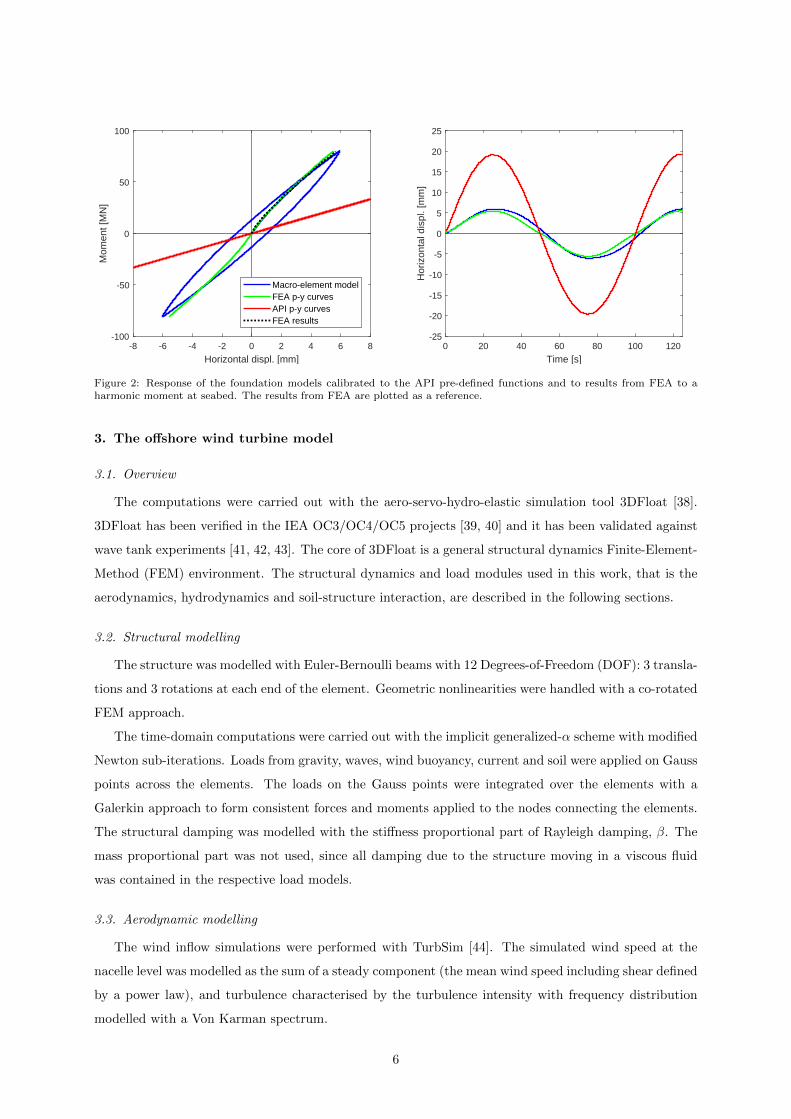
Figure 2: Response of the foundation models calibrated to the API pre-defined functions and to results from FEA to aharmonic moment at seabed. The results from FEA are plotted as a reference.

3. The offshore wind turbine model

3.1. Overview

The computations were carried out with the aero-servo-hydro-elastic simulation tool 3DFloat [38].

3DFloat has been verified in the IEA OC3/OC4/OC5 projects [39, 40] and it has been validated against

wave tank experiments [41, 42, 43]. The core of 3DFloat is a general structural dynamics Finite-Element-

Method (FEM) environment. The structural dynamics and load modules used in this work, that is the

aerodynamics, hydrodynamics and soil-structure interaction, are described in the following sections.

3.2. Structural modelling

The structure was modelled with Euler-Bernoulli beams with 12 Degrees-of-Freedom (DOF): 3 transla-

tions and 3 rotations at each end of the element. Geometric nonlinearities were handled with a co-rotated

FEM approach.

The time-domain computations were carried out with the implicit generalized-α scheme with modified

Newton sub-iterations. Loads from gravity, waves, wind buoyancy, current and soil were applied on Gauss

points across the elements. The loads on the Gauss points were integrated over the elements with a

Galerkin approach to form consistent forces and moments applied to the nodes connecting the elements.

The structural damping was modelled with the stiffness proportional part of Rayleigh damping, β. The

mass proportional part was not used, since all damping due to the structure moving in a viscous fluid

was contained in the respective load models.

3.3. Aerodynamic modelling

The wind inflow simulations were performed with TurbSim [44]. The simulated wind speed at the

nacelle level was modelled as the sum of a steady component (the mean wind speed including shear defined

by a power law), and turbulence characterised by the turbulence intensity with frequency distribution

modelled with a Von Karman spectrum.

6

The aerodynamic loads on the rotor blades were modelled with Blade Element Momentum theory

(BEM) with enhancements for dynamic inflow and yaw errors, as described in Bjorck [45]. For the idling

cases the rotor blades were pitched to feather. The generator characteristic had zero torque for low

revolutions per minute (rpm), and the rotor was therefore completely free to rotate.

The aerodynamic loads on the tower were modelled with quadratic drag.

3.4. Hydrodynamic modelling

The irregular wave kinematics were modelled as superposition of linear Airy waves for intermediate

water depth, according to the JONSWAP spectrum and wave spread modeled with the cos 2s approach,

as described in the DNV standards [35, 46]. No current was applied.

The hydrodynamic loads on the pile were modeled using the relative form of Morison’s equation

[47] with MacCamy-Fuchs corrections [48]. This means that the quadratic drag coefficient was modelled

frequency-independent, and that the frequency-dependent inertial loading, added mass and damping were

taken into account in a similar manner as in Linear Potential Theory, where the added mass at infinite

frequency is added to the mass matrix. The effect of frequency dependent added mass and damping

appears as forcing term, a convolution integral taking into account the history of motions.

3.5. Foundation modelling

Both the p-y curves and the macro-element models described in Section 2.2 were used to represent

the foundation behaviour in the numerical model of the OWT.

4. Validation with measurement data

4.1. Case study

The measurement data employed in the model validation correspond to an offshore wind turbine

structure located in the North Sea. The hub height of the OWT is 81.8 m above the lowest astronomical

tide (LAT). The transition piece is approximately 22 m high. The water depth is 21.9 m with respect

to LAT. The wind turbine is placed on a monopile foundation, with a diameter varying between 4.74

and 5.70 m, and a wall thickness varying between 50 and 77 mm. The pile toe is located 50.4 m below

LAT, leading to an embedded depth of 28.5 m. The soil consists of stiff clay with layers of dense sand.

The small strain shear modulus of the soil varies between 100 and 500 MPa along the pile, while the

undrained shear strength of the stiff clay varies between 50 and 300 kPa. The estimated friction angle of

the sand varies between 44 and 48 degrees. Fig. 3 provides and schematic view of the OWT dimensions

and soil layering.

From the available time histories of the tower response, three idling periods were selected. For these

cases, different wave and wind conditions, and different angles of misalignment between wind and waves

were encountered. Idling cases were chosen as the response of the entire OWT is more influenced by the

foundation performance during idling cases than during production cases [5].

In addition, sensitivity analyses were carried out in Section 6 to capture the impact on the results of

the wave loading due to uncertainties in the statistical wave parameters.

7

Accelerometers

Straingauges

Stiffclay

Densesand

Stiffclay

Seabed

LAT

102.7m

28.5m

4.7-5.7m

21.9m

Anemometer

Figure 3: Schematic view of the OWT dimensions, soil layering and measurements setup.

8

0 5 10 15 20 25 30

Time [s]

0

10

20

30

40W

ind

spee

d [m

/s]

(a) Wind speed at nacelle level.

0 5 10 15 20 25 30

Time [s]

-0.2

-0.1

0

0.1

0.2

FA

-acc

eler

atio

n [m

/s2]

(b) Acceleration at the tower bottom.

0 5 10 15 20 25 30

Time [s]

-20

-10

0

10

20

FA

-mom

ent [

MN

m]

(c) Moment at seabed.

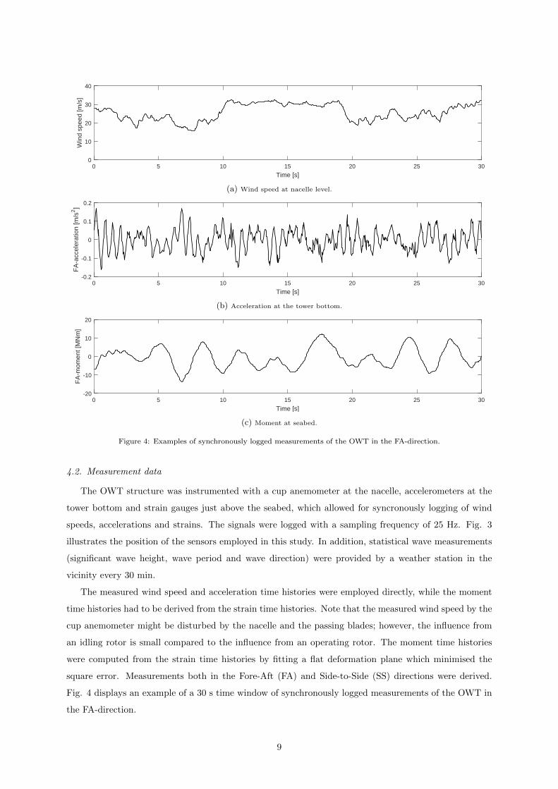
Figure 4: Examples of synchronously logged measurements of the OWT in the FA-direction.

4.2. Measurement data

The OWT structure was instrumented with a cup anemometer at the nacelle, accelerometers at the

tower bottom and strain gauges just above the seabed, which allowed for syncronously logging of wind

speeds, accelerations and strains. The signals were logged with a sampling frequency of 25 Hz. Fig. 3

illustrates the position of the sensors employed in this study. In addition, statistical wave measurements

(significant wave height, wave period and wave direction) were provided by a weather station in the

vicinity every 30 min.

The measured wind speed and acceleration time histories were employed directly, while the moment

time histories had to be derived from the strain time histories. Note that the measured wind speed by the

cup anemometer might be disturbed by the nacelle and the passing blades; however, the influence from

an idling rotor is small compared to the influence from an operating rotor. The moment time histories

were computed from the strain time histories by fitting a flat deformation plane which minimised the

square error. Measurements both in the Fore-Aft (FA) and Side-to-Side (SS) directions were derived.

Fig. 4 displays an example of a 30 s time window of synchronously logged measurements of the OWT in

the FA-direction.

9

4.3. Calibration of the numerical model

4.3.1. Structural model

The numerical model described in Section 3 was calibrated to the OWT structure described in Section

4.1. The finite element representation of the structure, displayed in Fig. 5, followed closely the detailed

drawings of the OWT. The cylinder and cone elements in 3DFloat were specified directly with diameter,

wall thickness and material properties. Equipment like ladders, J-tubes, bumpers and equipment in the

tower were represented as distributed mass per unit length or point masses. In addition, eigenvalue anal-

yses were performed with different element resolutions to ensure the structural response was independent

from element discretization.

The stiffness proportional β coefficient in the Rayleigh structural damping model was chosen to obtain

a damping ratio of 0.6% of critical at the first natural frequency. This value was chosen following the

structural damping calibrated in Shirzadeh et al. [23] to a similar OWT structure. Typical structural

damping ratios are in the range 0.5% and 1.5%, depending on whether additional damping sources, like

joints, are included [49]. Note that no tuning of the structure was performed in order to match the

measured natural frequencies.

4.3.2. Aerodynamic model

The calibration of the aerodynamic model requires parameters describing the deterministic and

stochastic wind properties for each case. For the deterministic wind speed, for the wind shear model, a

power law coefficient of 0.14 was assumed, and the average wind speeds listed in Table 1 were applied.

An air density of 1.225 kg/m3 was selected in all the cases. For the stochastic wind speed properties, the

turbulence intensities listed in Table 1 were employed.

The wind turbine rotor geometry and airfoil characteristics used in this paper were of a generic

design based on public information. The generic airfoil tables for the studied OWT were used without

modifications. Small adjustments on the controller settings and blade pitch angle were used to match

known properties of the rotor, such as rated rpm, rated power and thrust characteristics. For the idling

rotor cases described in this article, no further tuning was performed.

4.3.3. Hydrodynamic model

In the calibration of the hydrodynamic model, one has to specify the drag coefficient and the inertia

coefficient employed in Morison’s equation, together with the wave parameters. A drag coefficient of

1.10 was calculated based on the wave length and pile diameter, assuming a rough water-pile interface.

The inertia coefficient was calculated for each wave frequency using the MacCamy-Fuchs correction.

Input of significant wave height, wave peak period and wave direction were taken direcly from statistical

measurements listed in Table 1. A water density of 1025 kg/m3 was selected for all cases.

4.3.4. Foundation model

The two foundation models presented in Section 2.2 were calibrated to the approaches described in

Section 2.3 leading to the following combinations:

10

• API p-y curves. A p-y curve model that follows the API formulation for lateral loading of piles.

• FEA p-y curves. A p-y curve model calibrated to FEA of the soil and the foundation.

• Macro-element model. The macro-element model calibrated to FEA of the soil and the foundation.

Both the p-y curves model and the macro-element model were calibrated to results from FEA, since

this is considered the most accurate calibration approach. In addition, the p-y curves model were fitted

to the API p-y pre-defined functions. Despite p-y curves described by the API formulation generally

underestimate the foundation stiffness and natural frequency of the OWT, they were used in this study

because: (1) API p-y curves still represent the industry practice; (2) they were used in the initial design of

the OWT considered in the case study and (3) they have been used in comparable studies, e.g. Shirzadeh

et al. [23].

− 50 − 25 0 25 50y [m ]

Macro-elementmodel− 50

− 25

0

25

50

75

100

125

z [m

]

(a) Macro-element model

− 50 − 25 0 25 50y [m ]

FEAp-ycurves− 50

− 25

0

25

50

75

100

125

z [m

]

(b) FEA p-y curves

− 50 − 25 0 25 50y [m ]

APIp-ycurves− 50

− 25

0

25

50

75

100

125

z [m

]

(c) API p-y curves

Figure 5: Illustration of the finite element model of the OWT and sketch of the different foundation models.

The commercial software PLAXIS 3D described by Brinkgreve et al. [50] was employed to perform the

three-dimensional FEA. A mesh with roughly 200 000 10-noded tetrahedral soil elements was employed

with a denser discretization around the pile. Due to symmetry, only half of the geometry and the loads

were included. The pile was modelled as a solid volume with an equivalent stiffness, in a similar manner

as in Zdravkovic et al. [51], neglecting the stiffness of the soil plug. Pile installation effects were not

considered, and the pile was modelled as ’wished in place’ in initially undisturbed ground conditions.

The behaviour of the clay layers in the FEA was represented by the NGI-ADP soil model [52], which

describes the elasto-plastic, non-linear stress path dependent behaviour of saturated clays under undrained

monotonic loading conditions. The sand layers were represented with the Hardening Soil Small Strain

model [53], which captures the small strain soil stiffness and its non-linear dependency on the strain

amplitude. The constitutive model calibration was based on few direct simple shear and triaxial tests,

11

while the determination of the ε50 in the API formulation was derived from direct simple shear tests. For

the soil profile, best estimates of shear strength and shear modulus were selected. Note that the variability

in the soil properties around the best estimate was not considered in the calibration of foundation models.

The macro-element model was calibrated to the FEA load-displacement curves at the pile head fol-

lowing the procedure described in Page et al. [14]. The FEA p-y curves were extracted from the FEA

as follows. First, the bending moment along the pile and the lateral pile deflection were obtained at

different load levels. Then, the lateral resistance of the soil, p, was calculated at each depth as the second

derivative of the bending moment, and plotted against y. The resulting p-y curves where slightly tuned

to match perfectly the FEA results, and therefore the macro-element calibration. Fig. 2 compares the

results from FEA with the macro-element and the FEA p-y curves calibrations. Note that the three

curves overlap.

The added mass of the soil has been neglected in the foundation models. The added mass of the

soil is a simplified way to account for the frequency dependency of the foundation response. For typical

soil conditions found in offshore wind farms, the frequency dependency of the foundation response can

be neglected below a threshold value. For the OWT considered in this study, the threshold frequency

calculated with the formulae from Shadlou and Bhattacharya [54] is approximately 1.4 Hz. Given that

the measured first natural frequency of the OWT is approximately 0.33 Hz, most of the energy content

will be below the threshold, and therefore no noticeable frequency dependence is expected.

4.4. Simulations

The simulations were performed for 1800 seconds excluding transient parts. The different foundation

models required different time step sizes. Both the simulations with the macro-element model and with

API p-y curves were run with a step size of 0.01 s, while for the FEA p-y curves, a step size of 0.004 s was

employed. The computational times required to run one step were very similar for the macro-element

and for the p-y curves models. The p-y curves models were faster than the macro-element model with

respect to the computational time per step and per node. However, that was compensated by the number

of nodes required in each of the foundation models: in the simulations with the macro-element model,

only one node was needed to compute the foundation response, while in the simulations with p-y curves,

27 additional nodes representing the pile below seabed were required.

Separate tests on time step and element resolution were carried out to confirm that the simulated

response were not sensitive to resolution in time and space. In addition, for each idling case and for

each foundation model, 10 random seeds were generated. The simulated responses presented in Section

5 correspond to the average simulated response of the 10 seeds, plotted together with the maximum and

minimum simulated responses.

4.5. Comparison between measurements and simulations

In Section 5, a comparison between simulations and measurements is presented for the three idling

cases listed in Table 1. The simulated loads were computed employing the models presented in Section 3

calibrated to the parameters specified in Section 4.3. The same seeds (to model the turbulent wind and the

12

irregular waves) were employed for each case, so the results simulated with the different foundation models

are directly comparable. However, the comparison between the simulations and the measurements has

to be done in a qualitative manner, since the real environmental actions might differ from the simulated

actions. This is especially relevant for the simulated waves, since only wave statistics were available.

In the three idling cases considered, the rotor is facing the wind. This means that the fore-aft (FA)

direction is the wind direction and that the side-to-side (SS) direction is perpendicular to the wind. The

misalignment between wind and waves is therefore the angle between the wave direction and the FA

direction.

Table 1: Ambient conditions of the idling cases investigated

Case

number

Time

window

Wind

speed

Turbulence

intensity

Wave

height

Wave

period

Wind and wave

misalignment

[s] [m/s] [%] [m] [s] [degrees]

1 1800 7.94 16.46 1.20 5.26 6

2 1800 22.40 19.95 2.70 5.79 -50

3 1800 2.40 14.79 2.10 4.81 -86

4.6. Processing of the results

The measurements and the simulations are stochastic processes and cannot be compared directly in

the time domain. In order to draw a comparison, the same processing was applied to both the measured

and simulated time histories:

Fast Fourier Transform. The Fast Fourier Transform (FFT) was applied to both the accelerations and

moments to compute the Power Spectral Densisty (PSD) of the time histories. The PSD displays the

energy content of the system response at different frequencies. The time series were divided into intervals

with 50% overlap. The FFT was applied to each interval, and an average was calculated.

Root Mean Square. The Root Mean Square (RMS) of the acceleration signal was computed. Since the

measured and simulated accelerations have zero mean, the RMS is equivalent to the standard deviation.

Rainflow counting. Rainflow counting was applied to identify the main cycles and filter noise cycles in

the time-domain. It is a process that converts a random signal to a count of constant amplitude cycles.

It was employed to count the amplitude of the moments at the seabed, which was later plotted as a

probability of exceedance or employed to compute damage equivalent loads.

Cummulative probability of exceedance. The probability of exceedance calculates the probability that a

stochastic process may exceed some critical value, in this case the moment amplitude at the seabed. It was

calculated as follows: first, rainflow counting was applied to the moment time history, and the moment

amplitudes were sorted in increasing order. Then, the probability of exceedance was calculated as the

13

number of cycles that have a moment amplitude smaller than the critical value over the total number

of cycles in the time history. The probability of exceedance gives an indication of the distribution of

moment amplitudes in the simulations and the measurements.

1 Hz Damage Equivant Loads. The Damage Equivalent load is defined as the single-amplitude load that

causes the same amount of damage over a reference number of cycles Nk as the variable-amplitude load

time series Si with the corresponding number of cycles Ni

DEL =

(n∑

i=1

Ni

NkSmi

)1/m

(1)

Where n is the number of load ranges, and m is the inverse slope of the considered stress-cycle curve

(S −N curve) according to DNV [35]. The parameter m was set to 3.0. In the 1 Hz DEL, the reference

number of cycles Nk is calculated as the length of the time series times 1 Hz. A clear definition of DELs

can be found in Cosack [55].

5. Results and Discussion

5.1. Natural frequencies

This section compares the measured and simulated natural frequencies. The measured natural fre-

quencies were identified from the peaks of the Power Spectral Density (PSD) of the measured accelerations

at the tower bottom displayed in Fig. 6. The PSD was obtained from a 4800 seconds long idling case,

with an average wind speed of 9.4 m/s, an average wave height of 1.2 m and codirectional wind and waves.

The simulated natural frequencies were obtained from eigenvalue analyses in parked conditions, where

the blades were pitched to 90◦ and the rotor was locked, and for the three foundation models described

in Section 3.5. Included in Fig. 6 are vertical lines corresponding to the 10 lowest simulated natural

frequencies obtained with the macro-element model. The natural frequencies that directly relate to the

foundation modeling are the support structure bending frequencies. These are listed and visualized for

the three foundation models in Table 2, together with the measured values.

The measured natural frequencies agree well with the natural frequencies simulated with the macro-

element and with the FEA p-y curves. The simulation with API p-y curves underestimates the measured

first and second support structure natural frequencies by 11 % and by 18%, respectively. This agrees

with observations found in the literature. Kallehave et al. [56] and Zaaijer [57] compared the measured

first support structure natural frequency to the design frequency for monopile-based OWT modelled with

API p− y curves, and found that the natural frequency was generally underpredicted in the design, some

by more than 20%.

5.2. Wind speed at nacelle level

This section compares the measured and simulated wind speeds at the nacelle level in the FA direction,

both in the frequency and in the time-domain. Fig. 7 plots the comparison between the spectrum derived

14

10-1 100

Frequency [Hz]

10-8

10-6

10-4

10-2

PS

D o

f acc

eler

atio

n [(

m/s

2)/

Hz]

Measured accelerations in the FA-directionMeasured accelerations in the SS-directionSimulated support structure natural frequencies in the FA-directionSimulated support structure natural frequencies in the SS-directionSimulated blade bending frequencies

Figure 6: Comparison between the Power Spectral Density (PSD) of the measured accelerations and the 10 lowest naturalfrequencies simulated with the macro-element model.

Table 2: Comparison between the measured and the simulated natural frequencies for the first two tower modes

Measured

freq. (Hz)

Simulated freq. (Hz) Simulated modes

Macro-

element

model

FEA p-y

curves

API p-y

curvesFront view Side view Top view

1st Sup.

Struct. FA0.332 0.331 0.330 0.291

1st Sup.

Struct. SS0.336 0.335 0.334 0.293

2nd Sup.

Struct. FA1.650 1.670 1.661 1.322

2nd Sup.

Struct. SS1.650 1.677 1.667 1.339

from measurements and the Von Karman spectrum used in the simulations of Case 2. From the three

idling cases analysed, the simulated response in Case 2 is dominated by wind loading, while the responses

in Cases 1 and 3 are dominated by wave loading. Fig. 7 indicates that simulated wind speed agrees

reasonably well with the measured wind speeds up to the first support structure natural frequency, and

15

10-2 10-1 100 101

Frequency [Hz]

10-4

10-2

100

102

104

PS

D o

f win

d sp

eed

[(m

/s)

2/H

z]

MeasuredSimulated

Case 2

Figure 7: Power Spectral Density of the measured and simulated wind speed at the nacelle for Case 2.

it is overestimated for higher frequencies.

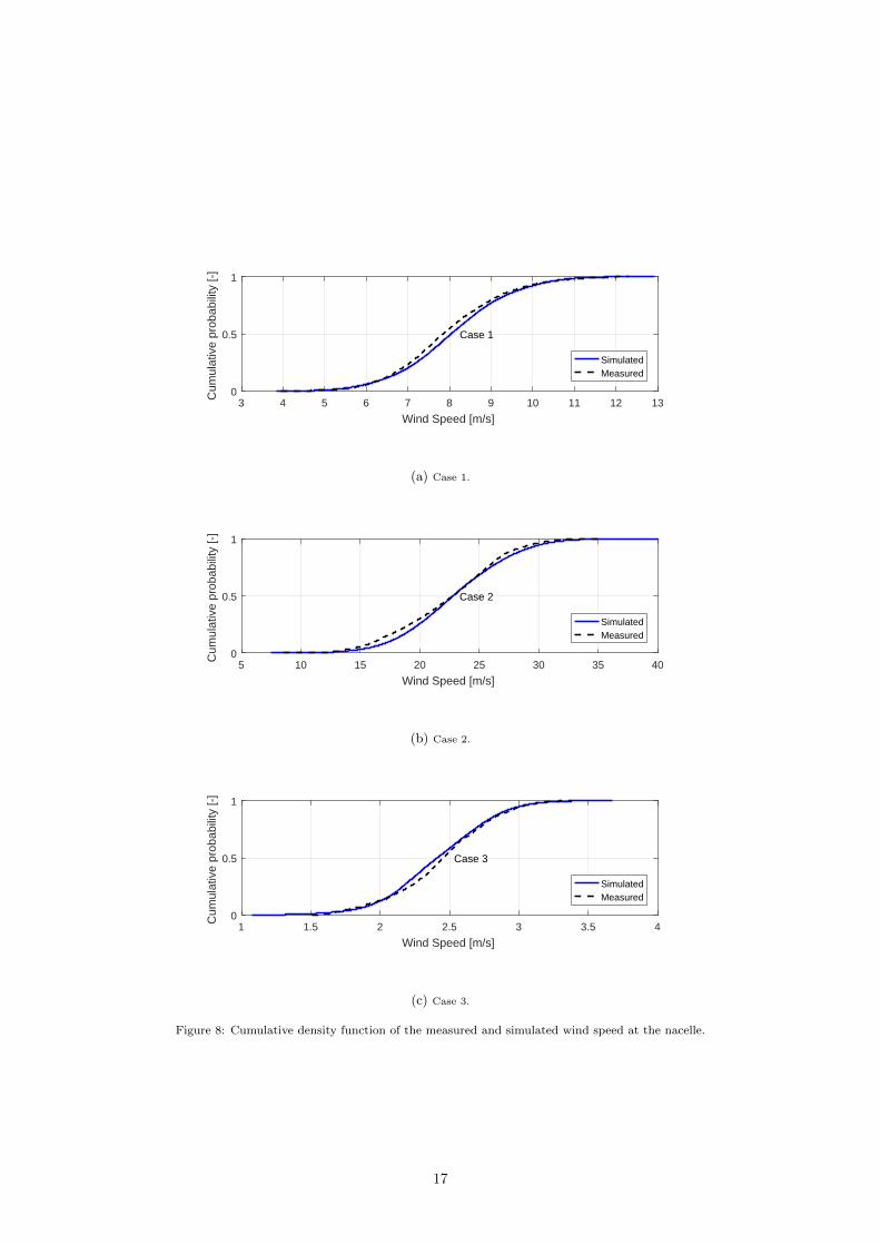
The cumulative density functions of the measured and simulated wind speeds are plotted in Fig. 8

for the three idling cases analysed. An acceptable agreement is found taking into account that the wind

speed is measured behind the rotor, and some disturbances in the wind inflow, and therefore in the wind

speed can be expected.

5.3. Accelerations at the tower bottom

Unlike the undamped natural frequencies, which depend only on the mass and stiffness properties

of the OWT and the soil conditions, the acceleration levels are determined also by the loads acting

on the structure. In the simulations, the loads acting on the structure were calculated based on the

available environmental measurements. Simulations with different foundation models used the same

wind and wave realisations, therefore, simulation results from different foundation models can be directly

compared to each other. However, the comparison between the measured and simulated accelerations

should be interpreted with caution, since the actual loads acting on the structure were not measured. It

is therefore not possible to know if the simulated actions were similar to the real actions. The impact of

the simulated actions on the structure was evaluated in the sensitivity study presented in Section 6.

The comparison between the accelerations at the tower bottom simulated (in the time domain) with

the different foundation models and the measurement data is presented by comparing spectra, in the

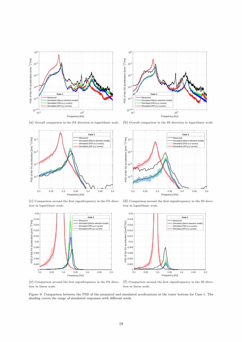
frequency domain, and by comparing the RMS. Figs. 9, 10 and 11 display, for the idling cases analysed,

the PSD of the measured and simulated acceleration at the tower bottom. First, subfigures (a) to (d) give

an overview of the PSD in logarithmic scale. Then, the details around the first tower bending frequency

are shown in (e) and (f) in linear scale. Note that the PSD in linear scale shows the contributions of

the different frequencies to the variance, and that the area under the PSD curves plotted in linear scale

16

3 4 5 6 7 8 9 10 11 12 13

Wind Speed [m/s]

0

0.5

1

Cum

ulat

ive

prob

abili

ty [-

]

Case 1

SimulatedMeasured

(a) Case 1.

5 10 15 20 25 30 35 40

Wind Speed [m/s]

0

0.5

1

Cum

ulat

ive

prob

abili

ty [-

]

Case 2

SimulatedMeasured

(b) Case 2.

1 1.5 2 2.5 3 3.5 4

Wind Speed [m/s]

0

0.5

1

Cum

ulat

ive

prob

abili

ty [-

]

Case 3

SimulatedMeasured

(c) Case 3.

Figure 8: Cumulative density function of the measured and simulated wind speed at the nacelle.

17

10-1 100

Frequency [Hz]

10-10

10-8

10-6

10-4

10-2

100

PS

D o

f the

FA

acc

eler

atio

n [(

m/s

2)2

/Hz]

MeasuredSimulated (Macro-element model)Simulated (FEA p-y curves)Simulated (API p-y curves)

Case 1

(a) Overall comparison in the FA direction in logarithmic scale.

10-1 100

Frequency [Hz]

10-10

10-8

10-6

10-4

10-2

100

PS

D o

f the

SS

acc

eler

atio

n [(

m/s

2)2

/Hz]


Case 1

(b) Overall comparison in the SS direction in logarithmic scale.

0.2 0.25 0.3 0.35 0.4 0.45 0.5

Frequency [Hz]

10-4

10-3

10-2

10-1

PS

D o

f the

FA

acc

eler

atio

n [(

m/s

2)2

/Hz] Measured

Simulated (Macro-element model)Simulated (FEA p-y curves)Simulated (API p-y curves)

Case 1

(c) Comparison around the first eigenfrequency in the FA direc-

tion in logarithmic scale.

0.2 0.25 0.3 0.35 0.4 0.45 0.5

Frequency [Hz]

10-4

10-3

10-2

10-1

PS

D o

f the

SS

acc

eler

atio

n [(

m/s

2)2

/Hz] Measured


Case 1

(d) Comparison around the first eigenfrequency in the SS direc-


0.2 0.25 0.3 0.35 0.4 0.45 0.5

Frequency [Hz]

0

0.002

0.004

0.006

0.008

0.01

0.012

0.014

0.016

0.018

0.02

PS

D o

f the

FA

acc

eler

atio

n [(

m/s

2)2

/Hz] Measured


Case 1

(e) Comparison around the first eigenfrequency in the FA direc-

tion in linear scale.

0.2 0.25 0.3 0.35 0.4 0.45 0.5

Frequency [Hz]

0

0.002

0.004

0.006

0.008

0.01

0.012

0.014

0.016

0.018

0.02

PS

D o

f the

SS

acc

eler

atio

n [(

m/s2

)2/H

z] MeasuredSimulated (Macro-element model)Simulated (FEA p-y curves)Simulated (API p-y curves)

Case 1

(f) Comparison around the first eigenfrequency in the SS direc-


Figure 9: Comparison between the PSD of the measured and simulated accelerations at the tower bottom for Case 1. Theshading covers the range of simulated responses with different seeds.

18

10-1 100

Frequency [Hz]

10-7

10-6

10-5

10-4

10-3

10-2

10-1

100

PS

D o

f the

FA

acc

eler

atio

n [(

m/s

2)2

/Hz]


Case 2


10-1 100

Frequency [Hz]

10-7

10-6

10-5

10-4

10-3

10-2

10-1

100

PS

D o

f the

SS

acc

eler

atio

n [(

m/s

2)2

/Hz]


Case 2


0.2 0.25 0.3 0.35 0.4 0.45 0.5

Frequency [Hz]

10-4

10-3

10-2

10-1

100

PS

D o

f the

FA

acc

eler

atio

n [(

m/s

2)2

/Hz] Measured


Case 2



0.2 0.25 0.3 0.35 0.4 0.45 0.5

Frequency [Hz]

10-4

10-3

10-2

10-1

100

PS

D o

f the

SS

acc

eler

atio

n [(

m/s

2)2

/Hz] Measured


Case 2



0.2 0.25 0.3 0.35 0.4 0.45 0.5

Frequency [Hz]

0

0.01

0.02

0.03

0.04

0.05

0.06

0.07

0.08

PS

D o

f the

FA

acc

eler

atio

n [(

m/s

2)2

/Hz] Measured


Case 2



0.2 0.25 0.3 0.35 0.4 0.45 0.5

Frequency [Hz]

0

0.01

0.02

0.03

0.04

0.05

0.06

0.07

0.08

PS

D o

f the

SS

acc

eler

atio

n [(

m/s2

)2/H


Case 2




relates to the RMS values. Table 3 lists the RMS values of the measured and simulated accelerations for

each of the idling cases analysed.

19

The comparison between the simulations with API p-y curves and with FEA p-y curves highlights the

effect of having different foundation stiffnesses. The only difference between the two simulations is the

calibration of the foundation model, which results in a lower foundation stiffness in the API p-y curves

model and a lower natural frequency. As a consequence, the position of the peaks corresponding to the

first and second support structure natural frequencies are found at lower frequencies in the PSD. Note

that the three foundation models predict the same blade natural frequencies. In addition, the acceleration

values are overpredicted, especially around the first natural frequency. This is because in the simulations

with API p-y curves, the support structure will undergo larger amounts of excitation of its fundamental

frequency from the wave spectrum. Moreover, larger displacements and accelerations are generated as a

consequence of the softer system.

The comparison between the FEA p-y curves and the macro-element model highlights the effect of

including foundation damping. Both the macro-element and FEA p-y curves models show very similar

foundation stiffness (see Fig. 2); however, the macro-element model includes hysteretic foundation damp-

ing in its formulation, while the FEA p-y curves do not. In overall, the difference between the PSD of

the accelerations at the tower bottom of the macro-element and the FEA p-y curves is small. This effect

is most visible in the peak corresponding to the first natural frequency.

In general, the comparison between the measurements and the simulations with the macro-element

model and FEA p-y curves is good, while the simulation results with API p-y curves do not agree well

with the measured spectra. Around the first support structure natural frequencies, the macro-element

model seems to agree with the measured accelerations better than the FEA p-y curves. A detailed

comparison between simulations and measurements reveals that:

• For frequencies higher than the first natural frequency, the simulated spectra are consistently lower

than the measured spectrum. This is because the structural damping was modelled proportional to

the frequency (as Rayleigh damping), while in reality the damping due to internal friction in steel

structures is fairly independent of frequency. In the simulations, the β parameter in the Rayleigh

damping model was selected to give a structural damping ratio of 0.6% at the first tower bending

frequency. This means that, at the second support structure natural frequency, the simulated

structural damping is 5 times larger than the selected value. Details at the second support structure

natural frequency could have been explored by re-running the simulations with a β parameter chosen

to give the correct structural damping at this frequency. However, an increase in accelerations

around this frequency would not have had a substantial contribution to the RMS, estimated from

the area under the curves in Figs. 9 to 11.

• In Case 2 (Fig. 10), the PSD of accelerations were not underestimated despite the overestimation of

structural damping at high frequencies. This is because the wind spectrum was also overestimated

at high frequencies, and the overestimation of structural damping compensated the overestimation

of the actions from the wind.

• In Case 1, the wave direction (from statistical data) is not consistent with the wave direction inferred

20

10-1 100

Frequency [Hz]

10-12

10-10

10-8

10-6

10-4

10-2

100

PS

D o

f the

FA

acc

eler

atio

n [(

m/s

2)2

/Hz]


Case 3


10-1 100

Frequency [Hz]

10-12

10-10

10-8

10-6

10-4

10-2

100

PS

D o

f the

SS

acc

eler

atio

n [(

m/s

2)2

/Hz]


Case 3


0.2 0.25 0.3 0.35 0.4 0.45 0.5

Frequency [Hz]

10-6

10-5

10-4

10-3

10-2

10-1

100

PS

D o

f the

FA

acc

eler

atio

n [(

m/s

2)2

/Hz] Measured


Case 3



0.2 0.25 0.3 0.35 0.4 0.45 0.5

Frequency [Hz]

10-6

10-5

10-4

10-3

10-2

10-1

100

PS

D o

f the

SS

acc

eler

atio

n [(

m/s

2)2

/Hz] Measured


Case 3



0.2 0.25 0.3 0.35 0.4 0.45 0.5

Frequency [Hz]

0

0.01

0.02

0.03

0.04

0.05

0.06

PS

D o

f the

FA

acc

eler

atio

n [(

m/s

2)2

/Hz] Measured


Case 3



0.2 0.25 0.3 0.35 0.4 0.45 0.5

Frequency [Hz]

0

0.01

0.02

0.03

0.04

0.05

0.06

PS

D o

f the

SS

acc

eler

atio

n [(

m/s2

)2/H


Case 3




21

from measured accelerations at the OWT. The measured accelerations in both FA and SS directions

(Fig. 9) are quite similar, which indicates that the misalignment between wind and waves might

be approximately 45◦. However a misalignment of only 6◦ was recorded in the statistical wave

measurements, and later used in the simulations. This might explain the overprediction of the FA

acceleration and the underprediction of the SS acceleration in Case 1.

Table 3: RMS values of the measured and simulated acelerations at the tower bottom for the different foundation models.

MeasuredSimulated

Macro-element model p-y curves from FEA API p-y curves

RMS RMS Difference to

measured

RMS Difference to

measured

RMS Difference to

measured[m/s2] [m/s2] [m/s2] [m/s2]

Case 1FA 0.0174 0.0158 -9% 0.0183 5% 0.0685 294%

SS 0.0175 0.0077 -56% 0.0085 -51% 0.0325 86%

Case 2FA 0.0438 0.0380 -13% 0.0452 3% 0.0816 86%

SS 0.0421 0.0389 -8% 0.0452 7% 0.0728 73%

Case 3FA 0.0193 0.0156 -19% 0.0187 -3% 0.0682 253%

SS 0.0171 0.0238 39% 0.0303 77% 0.1093 539%

Average -11% 6% 222%

Table 3 lists the RMS values of the measured and simulated accelerations for each of the idling cases

analysed. The difference between the measured RMS values and the RMS values of the simulations with

API p-y curves is similar to the difference found in Shirzadeh et al. [23]. Shirzadeh et al. [23] compared

RMS values of measured and simulated acelerations using API p-y curves in the foundation modelling,

and found that in general, the simulated accelerations were between a factor of two and three higher than

the measured accelerations.

5.4. Moments at seabed

This section presents a comparison between the measured and simulated moments at the seabed with

the different foundation models. The comparison is done both in the frequency domain, through the

PSD, and in the time domain, by the probability of exceedance of the cyclic moment.

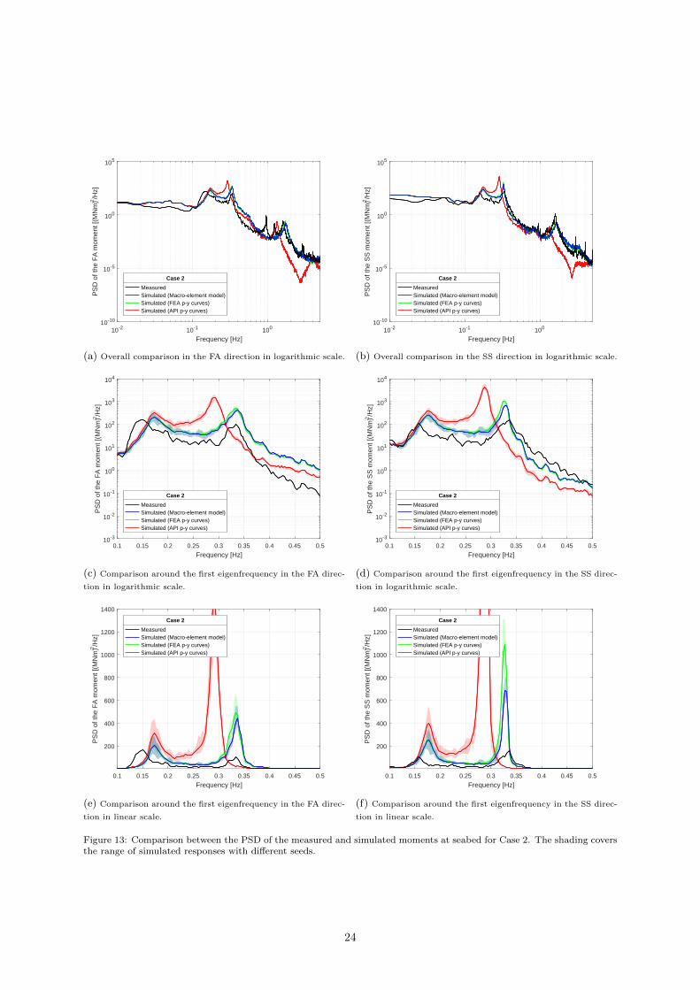
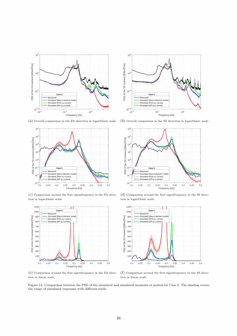
Figs. 12, 13 and 14 show the PSD of the measured and simulated moments at seabed for the three

foundations models and for Cases 1 to 3, respectively. Note that in the PSD of moments, the peak

corresponding to wave loading is more clear than in the PSD of accelerations. In addition, in the PSD of

moments, the peak corresponding to the second support structure natural frequency has relatively lower

energy content than in the PSD of accelerations, and therefore is less relevant for fatigue estimations.

The overall comparison between the measurements and simulations indicates that both the PSD

calculated with the macro-element and the FEA p-y curves agree well with the measurements, while the

simulations with API p-y curves predict a different dynamic response, which overpredicts the moment

amplitude. The simulations with the macro-element model predict lower moment amplitudes at the first

support structure natural frequency than the FEA p-y curves due to the presence of foundation damping.

A more detailed comparison between the simulations and measurements indicate that:

22

10-2 10-1 100

Frequency [Hz]

10-10

10-5

100

105

PS

D o

f the

FA

mom

ent [

(MN

m)2

/Hz]


Case 1


10-2 10-1 100

Frequency [Hz]

10-10

10-5

100

105

PS

D o

f the

SS

mom

ent [

(MN

m)2

/Hz]


Case 1


0.1 0.15 0.2 0.25 0.3 0.35 0.4 0.45 0.5

Frequency [Hz]

10-3

10-2

10-1

100

101

102

103

104

PS

D o

f the

FA

mom

ent [

(MN

m)2

/Hz]


Case 1



0.1 0.15 0.2 0.25 0.3 0.35 0.4 0.45 0.5

Frequency [Hz]

10-3

10-2

10-1

100

101

102

103

104

PS

D o

f the

SS

mom

ent [

(MN

m)2

/Hz]


Case 1



0.1 0.15 0.2 0.25 0.3 0.35 0.4 0.45 0.5

Frequency [Hz]

50

100

150

200

250

300

350

PS

D o

f the

FA

mom

ent [

(MN

m)2

/Hz]


Case 1



0.1 0.15 0.2 0.25 0.3 0.35 0.4 0.45 0.5

Frequency [Hz]

50

100

150

200

250

300

350

PS

D o

f the

SS

mom

ent [

(MN

m)2

/Hz]


Case 1



Figure 12: Comparison between the PSD of the measured and simulated moments at seabed for Case 1. The shading coversthe range of simulated responses with different seeds.

23

10-2 10-1 100

Frequency [Hz]

10-10

10-5

100

105

PS

D o

f the

FA

mom

ent [

(MN

m)2

/Hz]


Case 2


10-2 10-1 100

Frequency [Hz]

10-10

10-5

100

105

PS

D o

f the

SS

mom

ent [

(MN

m)2

/Hz]


Case 2


0.1 0.15 0.2 0.25 0.3 0.35 0.4 0.45 0.5

Frequency [Hz]

10-3

10-2

10-1

100

101

102

103

104

PS

D o

f the

FA

mom

ent [

(MN

m)2

/Hz]


Case 2



0.1 0.15 0.2 0.25 0.3 0.35 0.4 0.45 0.5

Frequency [Hz]

10-3

10-2

10-1

100

101

102

103

104

PS

D o

f the

SS

mom

ent [

(MN

m)2

/Hz]


Case 2



0.1 0.15 0.2 0.25 0.3 0.35 0.4 0.45 0.5

Frequency [Hz]

200

400

600

800

1000

1200

1400

PS

D o

f the

FA

mom

ent [

(MN

m)2

/Hz]


Case 2



0.1 0.15 0.2 0.25 0.3 0.35 0.4 0.45 0.5

Frequency [Hz]

200

400

600

800

1000

1200

1400

PS

D o

f the

SS

mom

ent [

(MN

m)2

/Hz]


Case 2




24

• The peak fequency corresponding to the wave excitation in the PSD does not agree with the peak

spectral frequency used in the simulated JONSWAP spectrum, which is based on statistical wave

measurements.

• The main wave direction from statistical measurements does not agree well with the direction in-

ferred from the measured acceleration and moments. This is specially relevant for Case 1, where

this diagreement leads to an overprediction of the moments in the FA direction and to an under-

prediction of the moments in the SS direction.

This suggests that the measured wave statistical data, which was employed as input to the numerical

model, might not represent the wave conditions at the exact OWT location.

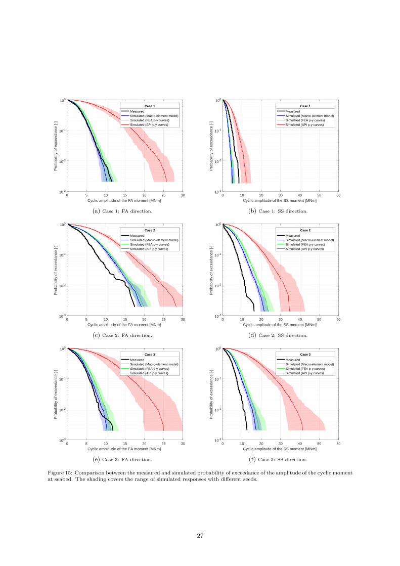
These conclusions are confirmed by looking at the probability of exceedance of the cyclic amplitude

of the moment at seabed displayed in Fig. 15. The results from both the macro-element model and the

FEA p-y curves agree well with the measurements, while the API p-y curves overpredict the moment

at the seabed by a factor of 2 to 3. This is in agreement with observations from Hald et al. [58]. Hald

et al. [58] compared the simulated and measured moments at different locations along the pile and found

that, close to the seabed, the measured moments were significantly smaller than the moments estimated

using API p-y curves. In addition, the macro-element model computes lower moments than the FEA p-y

curves, due to foundation damping. This effect is larger for the larger cyclic moment amplitudes.

5.5. Damage Equivalent Loads

A simplified but common way to compare the effect of the measured and simulated moments on the

fatigue, is by comparing the 1 Hz Damage Equivalent Loads (DELs). Table 4 lists the 1 Hz DEL of the

measured and simulated moments at seabed.

Table 4: 1 Hz Damage Equivalent Loads (DEL) of the measured and simulated moment at seabed for the different foundationmodels.

MeasuredSimulated

Macro-element model FEA p-y curves API p-y curves

1 Hz DEL 1 Hz DEL Difference to

measured

1 Hz DEL Difference to

measured

1 Hz DEL Difference to

measured[MNm] [MNm] [MNm] [MNm]

Case 1FA 2.96 3.07 4% 3.38 14% 8.62 191%

SS 2.46 1.51 -39% 1.58 -36% 3.95 61%

Case 2FA 4.29 5.62 31% 5.88 37% 8.25 92%

SS 4.09 5.88 44% 6.53 60% 10.79 164%

Case 3FA 2.88 3.12 8% 3.51 22% 8.44 193%

SS 3.48 5.01 44% 5.59 61% 13.77 296%

Average 15% 26% 166%

The comparison between the measured and simulated DELs indicates that the DELs are overpredicted

in the simulations. Note that measurements and simulations can only be compared in a qualitative

manner, since the simulated and real environmental actions might be different. However, the following

observations can be highlighted:

• The API p-y curves overestimate the DELs by a factor between 2 and 4 (166% on the average).

25

10-2 10-1 100

Frequency [Hz]

10-10

10-5

100

105

PS

D o

f the

FA

mom

ent [

(MN

m)2

/Hz]


Case 3


10-2 10-1 100

Frequency [Hz]

10-10

10-5

100

105

PS

D o

f the

SS

mom

ent [

(MN

m)2

/Hz]


Case 3


0.1 0.15 0.2 0.25 0.3 0.35 0.4 0.45 0.5

Frequency [Hz]

10-3

10-2

10-1

100

101

102

103

104

PS

D o

f the

FA

mom

ent [

(MN

m)2

/Hz]


Case 3



0.1 0.15 0.2 0.25 0.3 0.35 0.4 0.45 0.5

Frequency [Hz]

10-3

10-2

10-1

100

101

102

103

104

PS

D o

f the

SS

mom

ent [

(MN

m)2

/Hz]


Case 3



0.1 0.15 0.2 0.25 0.3 0.35 0.4 0.45 0.5

Frequency [Hz]

100

200

300

400

500

600

700

800

900

1000

1100

PS

D o

f the

FA

mom

ent [

(MN

m)2

/Hz]


Case 3



0.1 0.15 0.2 0.25 0.3 0.35 0.4 0.45 0.5

Frequency [Hz]

100

200

300

400

500

600

700

800

900

1000

1100

PS

D o

f the

SS

mom

ent [

(MN

m)2

/Hz]


Case 3




26

0 5 10 15 20 25 30

Cyclic amplitude of the FA moment [MNm]

10-3

10-2

10-1

100

Pro

babi

lity

of e

xcee

danc

e [-

]


Case 1

(a) Case 1: FA direction.

0 10 20 30 40 50 60

Cyclic amplitude of the SS moment [MNm]

10-3

10-2

10-1

100

Pro

babi

lity

of e

xcee

danc

e [-

]


Case 1

(b) Case 1: SS direction.

0 5 10 15 20 25 30


10-3

10-2

10-1

100

Pro

babi

lity

of e

xcee

danc

e [-

]


Case 2

(c) Case 2: FA direction.

0 10 20 30 40 50 60


10-3

10-2

10-1

100

Pro

babi

lity

of e

xcee

danc

e [-

]


Case 2

(d) Case 2: SS direction.

0 5 10 15 20 25 30


10-3

10-2

10-1

100

Pro

babi

lity

of e

xcee

danc

e [-

]


Case 3

(e) Case 3: FA direction.

0 10 20 30 40 50 60


10-3

10-2

10-1

100

Pro

babi

lity

of e

xcee

danc

e [-

]


Case 3

(f) Case 3: SS direction.

Figure 15: Comparison between the measured and simulated probability of exceedance of the amplitude of the cyclic momentat seabed. The shading covers the range of simulated responses with different seeds.

27

• The FEA p-y curves, which have the same formulation as the API p-y curves, but different calibra-

tion, overestimate the measured DEL by 26% on the average. The difference between the prediction

with API p-y curves and the prediction with FEA p-y curves highlights the effect of an accurate

calibration.

• The macro-element overetimates the measured DEL by 15% on the average. The difference of

roughly 10% between the macro-element model and the FEA p-y curves is due to the foundation

damping.

The comparison between the measured and simulated DELs gives some indication of the impact of

the foundation modelling on the fatigue. However, three idling cases are not enough to conclude about

the effect of the foundation models on the fatigue lifetime of the OWT. A complete fatigue assessment

requires consideration of the environmental conditions acting on the OWT during its lifetime. In order

to understand the effect of using the macro-element model vs. FEA p-y curves on the fatigue lifetime,

Næss [34] carried out a study on the OWT described in Section 4. The environmental conditions from

the UpWind design basis [59], corresponding to a site located in the North Sea, were employed to

cover the whole design lifetime. The study concluded that the fatigue damage over the lifetime of the

OWT simulated with the macro-element model was 22% lower than the fatigue damage over the lifetime

computed using FEA p-y curves.

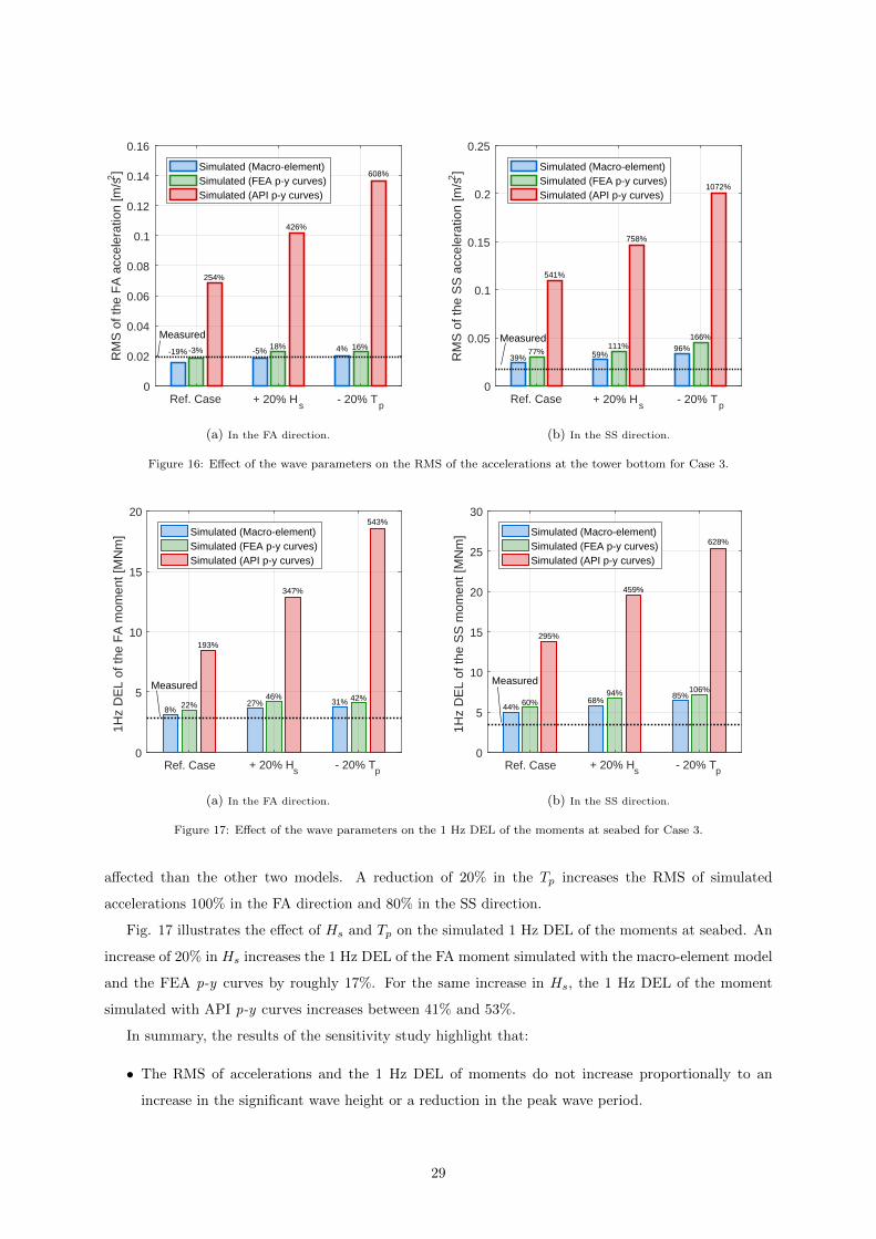
6. Sensitivity study on the wave parameters

This section presents and discusses the results from a sensitivity study on the significant wave height,

Hs, and peak wave period, Tp for Case 3. The effect of the wave parameters was investigated because:

(1) Shirzadeh et al. [23] found that Hs and Tp are the parameters that have the largest impact on

the vibration levels; (2) the Tp from the statistical wave measurements does not always agree will the

peak corresponding to the wave spectral peak in the PSD of moments, which indicates that the waves

measured in the vicinity of the OWT do not represent the wave conditions at the exact OWT location;

and (3) Shirzadeh et al. [23] showed that the wind parameters did not affect the RMS of accelerations

substantially.

Fig. 16 illustrates the effect of the significant wave height, Hs and wave peak period, Tp on the

simulated RMS of the accelerations at the tower bottom. An increase of 20% in Hs leads to an increase

between 14% to 18% in the RMS accelerations simulated using the macro-element model and the FEA

p-y curves. The model with API p-y curves is more sensitive to an increase in Hs. An increase of 20%

in Hs leads to an increase in the RMS of simulated accelerations of 48% in the FA direction and 33% in

the SS direction. In these simulations, the same seeds were used for all foundation models.

The reduction of 20% in Tp has larger impact on the simulated RMS of accelerations that an increase

of 20% in Hs. The RMS accelerations simulated with the macro-element model increases 28% in the

FA-direction and 41% in the SS-direction, while the RMS of accelerations simulated with FEA p-y curves

increases 16% in the FA-direction and 47% in the SS-direction. The model with API p-y curves is more

28

Ref. Case + 20% Hs

- 20% Tp

0

0.02

0.04

0.06

0.08

0.1

0.12

0.14

0.16

RM

S o

f the

FA

acc

eler

atio

n [m

/s2]

-19% -5% 4%-3% 18% 16%

254%

426%

608%

Measured

Simulated (Macro-element)Simulated (FEA p-y curves)Simulated (API p-y curves)

(a) In the FA direction.

Ref. Case + 20% Hs

- 20% Tp

0

0.05

0.1

0.15

0.2

0.25

RM

S o

f the

SS

acc

eler

atio

n [m

/s2]

39% 59%96%77%

111%166%

541%

758%

1072%

Measured


(b) In the SS direction.

Figure 16: Effect of the wave parameters on the RMS of the accelerations at the tower bottom for Case 3.

Ref. Case + 20% Hs - 20% Tp

0

5

10

15

20

1Hz

DE

L of

the

FA

mom

ent [

MN

m]

8%27% 31%22%

46% 42%

193%

347%

543%

Measured


(a) In the FA direction.

Ref. Case + 20% Hs - 20% Tp

0

5

10

15

20

25

30

1Hz

DE

L of

the

SS

mom

ent [

MN

m]

44%68%

85%60%

94% 106%

295%

459%

628%

Measured


(b) In the SS direction.

Figure 17: Effect of the wave parameters on the 1 Hz DEL of the moments at seabed for Case 3.

affected than the other two models. A reduction of 20% in the Tp increases the RMS of simulated

accelerations 100% in the FA direction and 80% in the SS direction.

Fig. 17 illustrates the effect of Hs and Tp on the simulated 1 Hz DEL of the moments at seabed. An

increase of 20% in Hs increases the 1 Hz DEL of the FA moment simulated with the macro-element model

and the FEA p-y curves by roughly 17%. For the same increase in Hs, the 1 Hz DEL of the moment

simulated with API p-y curves increases between 41% and 53%.

In summary, the results of the sensitivity study highlight that:

• The RMS of accelerations and the 1 Hz DEL of moments do not increase proportionally to an

increase in the significant wave height or a reduction in the peak wave period.

29

• Variations in the wave parameters affect signficantly the simulated RMS of accelerations and the 1

Hz DEL of moments, however, not as much as the difference between the API p-y curves and the

macro-element model and the FEA p-y curves.

• The API p-y curves model is more sensitive to a change in wave parameters than the macro-

element and the FEA p-y curves models. This is because in the simulations with API p-y curves,

the support structure will undergo larger amounts of excitation of its fundamental frequency from

the wave spectrum. Note that the difference between the first support natural frequency computed

with API p-y curves and computed with the macro-element and the FEA p-y curves is 11%.

7. Conclusions

This paper investigates the effect of the foundation model on the predicted response of a monopile-

based OWT installed in the North Sea by comparing simulations and full-scale field data. Measurements

of wind speed at nacelle level, accelerations at the tower bottom and moments at the seabed are used in

the comparison. The OWT structure and the environmental actions are implemented in the aero-servo-

hydro-elastic code 3DFloat. In the simulations, two foundation models (p-y curves and a macro-element

model) and two calibration approaches (API formulation and FEA) are evaluated, leading to the following

combinations: API p-y curves, FEA p-y curves and macro-element calibrated to FEA.

The comparison between the measured and simulated natural frequencies highlights the impact of

the calibration of the foundation model. The two foundation models calibrated to the results from

FEA provide accurate first and second support structure natural frequencies, while the foundation model

calibrated to the API formulation underpredicts the first and second natural frequencies by 11 and 18%,

respectively. Due to this difference, the simulations with API p-y curves predict a different dynamic

response than the measured and simulated response with the FEA p-y curves and macro-element models.

The comparison between the RMS of measured and simulated accelerations shows that the simulated

accelerations with API p-y curves overpredict the measured accelerations between a factor of two and

three. This is consistent with the findings from Shirzadeh et al. [23]. The simulated accelerations with the

macro-element model underpredict the measured accelerations by 11% in average, while the simulated

accelerations with FEA p-y curves overpredict the measured accelerations by 8% in average. This occurs

even when both foundation models give accurate predictions of the natural frequencies. It is believed

that it is due to an underprediction of the wave forces due to uncertain wave parameters. Note that the

difference between the macro-element model and FEA p-y curves is due to the generation of damping.

The comparison between the moments at the seabed indicate that the simulations overpredict the

measured moments for the three foundation models. This is considered conservative. The average differ-

ences between the measured and simulated 1 Hz DELs are as follows: macro-element model (15%), FEA

p-y curves (26%) and API p-y curves (166%). The difference between the API and the FEA p-y curves

illustrates the impact of an accurate calibration of the foundation model, while the difference between

the FEA p-y curves and the macro-element model highlights the impact of foundation damping. An

accurate prediction of the 1 Hz DEL of the moment gives an indication on how accurate the prediction

30

of the fatigue lifetime could be. In this regard, the simulations with the macro-element model calibrated

to FEA give the most accurate prediction. An accurate fatigue prediction is crucial for the OWT design,

since often the support structure design is fatigue-driven, where wave-induced fatigue in idling conditions

due to missing aero-elastic damping is frequently the main design driver.

In addition, the impact of the wave parameters on the simulated response is investigated in a sensitivity

study. The wave parameters have a large impact on the simulated accelerations and moments. However,

the impact of the foundation model calibration seems to be more important than an increase of 20% in

the significant wave height or a reduction of 20% in the peak wave period.

It is important to acknowledge the limitations of this study while interpreting the results. A single

OWT was studied, and only idling cases were considered. The simulated waves were based on statistical

wave measurements obtained from a weather station in the vicinity of the OWT. Comparison between

the statistical measurements and the acceleration and moments at the OWT suggested that the measured

wave statistical data might not represent the wave conditions at the exact OWT location. This might

explain some of the discrepancies between the simulated and measured responses.

Despite these limitations, this paper shows that, with a conceptually correct foundation model and a

realistic calibration, it is possible to match the measured natural frequency and predict accurate fatigue

loads. An accurate foundation model is not only important to estimate the fatigue lifetime of OWTs,

but also to avoid cost related to disagreements between designed and measured natural frequencies, such

as the engineering cost of re-evaluating the project certification loads or costs related to re-tuning of the

control system.

8. Acknowledgements

The financial support by the Norwegian Research Council through the project Reducing cost of off-

shore wind by integrated structural and geotechnical design (REDWIN), Grant No. 243984, is gratefully

acknowledged. We also would like to aknowledge Amir M. Kaynia and Hans Petter Jostad for their valu-

able comments during the development of the research and the writing of the paper, Kristoffer Skjolden

Skau for calibrating the soil parameters to the finite element model, Karin Noren-Cosgriff for support

with the measurements, and Alvaro Page for helping with the paper structure.

References

[1] A. Gazzo, F. Matzen, C. Farhangi, A. Lamdaouar, Offshore wind in Europe - Walking the tightrope

to success, Technical Report, Ernst & Young, 2015.

[2] I. R. TCP, Comparative Analysis of International Offshore Wind Energy Development (REWind Off-

shore), Technical Report, IEA Renewable Energy Technology Deployment Technology Collaboration

Programme (IEA RETD TCP), 2017.

31

[3] F. Vorpahl, H. Schwarze, T. Fischer, M. Seidel, J. Jonkman, Offshore wind turbine environment,

loads, simulation, and design, Wiley Interdisciplinary Reviews: Energy and Environment 2 (2013)

548–570.

[4] S. Schafhirt, A. Page, G. R. Eiksund, M. Muskulus, Influence of soil parameters on the fatigue

lifetime of offshore wind turbines with monopile support structure, Energy Procedia 94 (2016)

347–356.

[5] S. Aasen, A. M. Page, K. S. Skau, T. A. Nygaard, Effect of foundation modelling on the fatigue

lifetime of a monopile-based offshore wind turbine, Wind Energy Science 2 (2017) 361.

[6] API, Recommended Practice 2A-WSD. Planning, Designing, and Constructing Fixed Offshore Plat-

forms - Working Stress Design, 22 ed., American Petroleum Institute, 2014.

[7] M. Arshad, B. C. O’Kelly, Analysis and design of monopile foundations for offshore wind-turbine

structures, Marine Georesources & Geotechnology 34 (2016) 503–525.

[8] K. Lesny, Foundations for offshore wind turbines: tools for planning and design, VGE Verlag GmbH,

2010.

[9] P. Doherty, K. Gavin, Laterally loaded monopile design for offshore wind farms, Proceedings of the

Institution of Civil Engineers 165 (2011) 7–17.

[10] D. Kallehave, C. L. Thilsted, M. Liingaard, et al., Modification of the API p-y formulation of initial

stiffness of sand, in: Offshore Site Investigation and Geotechnics: Integrated Technologies-Present

and Future, Society of Underwater Technology, 2012.

[11] B. Byrne, R. McAdam, H. Burd, G. Houlsby, C. Martin, L. Zdravkovic, D. Taborda, D. Potts,

R. Jardine, M. Sideri, et al., New design methods for large diameter piles under lateral loading for

offshore wind applications, in: 3rd International Symposium on Frontiers in Offshore Geotechnics

(ISFOG 2015), Oslo, Norway, June, 2015, pp. 10–12.

[12] M. Damgaard, V. Zania, L. V. Andersen, L. B. Ibsen, Effects of soil-structure interaction on real

time dynamic response of offshore wind turbines on monopiles, Engineering Structures 75 (2014)

388–401.

[13] W. Beuckelaers, H. Burd, G. Houlsby, Integrated design method of monopile foundations for offshore

wind turbines using a kinematic hardening soil model, in: Proceedings of OSIG 2017 Conference,

Society for Underwater Technology, 2017.

[14] A. M. Page, G. Grimstad, G. R. Eiksund, H. P. Jostad, A macro-element pile foundation model for

integrated analyses of monopile-based offshore wind turbines, Ocean Engineering 167 (2018) 23 –

35.

[15] H. Matlock, Correlations for design of laterally loaded piles in soft clay, Offshore technology in civil

engineerings hall of fame papers from the early years (1970) 77–94.

32

[16] W. R. Cox, L. C. Reese, B. R. Grubbs, et al., Field testing of laterally loaded piles in sand, in:

Offshore Technology Conference, Offshore Technology Conference, 1974.

[17] L. C. Reese, W. R. Cox, F. D. Koop, et al., Field testing and analysis of laterally loaded piles in

stiff clay, in: Offshore Technology Conference, Offshore Technology Conference, 1975.

[18] B. Byrne, R. McAdam, H. Burd, G. Houlsby, C. Martin, W. Beuckelaer, L. Zdravkovic, D. Taborda,

D. Potts, R. Jardine, et al., PISA: new design methods for offshore wind turbine monopiles, in:

Proceedings of the Society for Underwater Technology Offshore Site Investigation and Geotechnics

8th International Conference on Smarter Solutions for Future Offshore Developments, 2017.

[19] N. J. Tarp-Johansen, L. Andersen, E. D. Christensen, C. Mørch, S. Frandsen, B. Kallesøe, Comparing

sources of damping of cross-wind motion, in: The European Offshore Wind Conference & Exhibition,

The European Wind Energy Association, 2009.

[20] W. De Vries, W. Versteijlen, A. Metrikine, J. Hoving, E. Smidt, Estimation of the vibration decre-

ment of an offshore wind turbine support structure caused by its interaction with soil, in: Proceedings

of the EWEA Offshore 2011 Conference, Amsterdam, The Netherlands, 29 November-1 December

2011, European Wind Energy Association, 2011.

[21] M. Damgaard, L. B. Ibsen, L. V. Andersen, J. Andersen, Cross-wind modal properties of offshore

wind turbines identified by full scale testing, Journal of Wind Engineering and Industrial Aerody-

namics 116 (2013) 94–108.

[22] C. Devriendt, P. J. Jordaens, G. De Sitter, P. Guillaume, Damping estimation of an offshore wind

turbine on a monopile foundation, IET Renewable Power Generation 7 (2013) 401–412.

[23] R. Shirzadeh, W. Weijtjens, P. Guillaume, C. Devriendt, The dynamics of an offshore wind turbine

in parked conditions: a comparison between simulations and measurements, Wind Energy 18 (2015)

1685–1702.

[24] B. Byrne, G. Houlsby, Foundations for offshore wind turbines, Philosophical Transactions of the

Royal Society of London A: Mathematical, Physical and Engineering Sciences 361 (2003) 2909–2930.

[25] A. M. Page, S. Schafhirt, G. R. Eiksund, K. S. Skau, H. P. Jostad, H. Sturm, et al., Alternative

numerical pile foundation models for integrated analyses of monopile-based offshore wind turbines, in:

The 26th International Ocean and Polar Engineering Conference, International Society of Offshore

and Polar Engineers, 2016.

[26] G. Houlsby, M. Cassidy, A plasticity model for the behaviour of footings on sand under combined

loading, Geotechnique 52 (2002) 117–129.

[27] B. Bienen, B. Byrne, G. Houlsby, M. Cassidy, Investigating six-degree-of-freedom loading of shallow

foundations on sand, Geotechnique 56 (2006) 367–379.

33

[28] C. Cremer, A. Pecker, L. Davenne, Cyclic macro-element for soil–structure interaction: material

and geometrical non-linearities, International Journal for Numerical and Analytical Methods in

Geomechanics 25 (2001) 1257–1284.

[29] K. S. Skau, G. Grimstad, A. M. Page, G. R. Eiksund, H. P. Jostad, A macro-element for integrated

time domain analyses representing bucket foundations for offshore wind turbines, Marine Structures

59 (2018) 158–178.

[30] V. Krathe, A. Kaynia, Implementation of a non-linear foundation model for soil-structure interaction

analysis of offshore wind turbines in FAST, Wind Energy 20 (2017) 695–712.

[31] A. M. Page, K. S. Skau, H. P. Jostad, G. R. Eiksund, A new foundation model for integrated analyses

of monopile-based offshore wind turbines, Energy Procedia 137 (2017) 100 – 107. 14th Deep Sea

Offshore Wind R&D Conference, EERA DeepWind’2017.

[32] A. Correia, A pile-head macro-element approach to seismic design of monoshaft-supported bridges,

Ph.D. thesis, European School for Advanced Studies in Reduction of Seismic Risk (ROSE School),

Pavia, Italy, 2011.

[33] Z. Li, P. Kotronis, S. Escoffier, C. Tamagnini, A hypoplastic macroelement for single vertical piles

in sand subject to three-dimensional loading conditions, Acta Geotechnica 11 (2016) 373–390.

[34] V. Næss, Optimization of Piles Supporting Monopile-Based Offshore Wind Turbines by Improved

Foundation Models, Master’s thesis, Norwegian University of Science and Technology, 2018.

[35] DNV, Design of offshore wind turbine structures - Offshore Standard DNV-OS-J101, DNV GL AS,

2014.

[36] K. Lesny, J. Wiemann, Finite-element-modelling of large diameter monopiles for offshore wind energy

converters, in: GeoCongress 2006: Geotechnical Engineering in the Information Technology Age,

2006, pp. 1–6.

[37] DNV, Support structures for wind turbines - Standard DNVGL-ST-0126, DNV GL AS, 2016.

[38] T. A. Nygaard, J. De Vaal, F. Pierella, L. Oggiano, R. Stenbro, Development, verification and

validation of 3DFloat; aero-servo-hydro-elastic computations of offshore structures, Energy Procedia

94 (2016) 425–433.

[39] W. Popko, F. Vorpahl, A. Zuga, M. Kohlmeier, J. Jonkman, A. Robertson, T. J. Larsen, A. Yde,

K. Saetertro, K. M. Okstad, et al., Offshore code comparison collaboration continuation (OC4),

Phase I-results of coupled simulations of an offshore wind turbine with jacket support structure:

Preprint, Technical Report, National Renewable Energy Lab.(NREL), Golden, CO (United States),

2012.

34

[40] A. Robertson, J. Jonkman, F. Vorpahl, W. Popko, J. Qvist, L. Frøyd, X. Chen, J. Azcona,

E. Uzunoglu, C. G. Soares, et al., Offshore code comparison collaboration continuation within

IEA wind task 30: Phase II results regarding a floating semisubmersible wind system, in: ASME

2014 33rd International Conference on Ocean, Offshore and Arctic Engineering, American Society

of Mechanical Engineers, 2014, pp. V09BT09A012–V09BT09A012.

[41] A. Myhr, T. A. Nygaard, Comparison of experimental results and computations for tension-leg-buoy

offshore wind turbines, Journal of Ocean and Wind Energy (2015).

[42] J. Azcona, F. Bouchotrouch, M. Gonzalez, J. Garciandıa, X. Munduate, F. Kelberlau, T. A. Nygaard,

Aerodynamic thrust modelling in wave tank tests of offshore floating wind turbines using a ducted

fan, in: Journal of Physics: Conference Series, volume 524, IOP Publishing, 2014, p. 012089.

[43] A. N. Robertson, F. F. Wendt, J. M. Jonkman, W. Popko, F. Vorpahl, C. T. Stansberg, E. E.

Bachynski, I. Bayati, F. Beyer, J. B. de Vaal, et al., OC5 project Phase I: validation of hydrody-

namic loading on a fixed cylinder, in: The Twenty-fifth International Ocean and Polar Engineering

Conference, International Society of Offshore and Polar Engineers, 2015.

[44] B. J. Jonkman, TurbSim user’s guide: Version 1.50, Technical Report, National Renewable Energy

Lab.(NREL), Golden, CO (United States), 2009.

[45] A. Bjorck, AERFORCE: Subroutine Package for unsteady Blade-Element/Momentum Calculations,

FFA Technical Note 2000-7 (2000).

[46] DNV, Environmental conditions and environmental loads - Recommended Practice DNVGL-RP-

C205, DNV GL AS, 2014.

[47] T. Sarpkaya, M. Isaacson, Mechanics of wave forces on offshore structures (1981).

[48] R. MacCamy, R. A. Fuchs, Wave forces on piles: a diffraction theory, Technical Report, Corps of

Engineers Washington DC Beach Erosion Board, 1954.

[49] R. Shirzadeh, C. Devriendt, M. A. Bidakhvidi, P. Guillaume, Experimental and computational

damping estimation of an offshore wind turbine on a monopile foundation, Journal of Wind Engi-

neering and Industrial Aerodynamics 120 (2013) 96–106.

[50] R. Brinkgreve, S. Kumarswamy, W. Swolfs, PLAXIS 2015. Reference Manual, Plaxis bv, 2015.

[51] L. Zdravkovic, D. Taborda, D. Potts, R. Jardine, M. Sideri, F. Schroeder, B. Byrne, R. McAdam,

H. Burd, G. Houlsby, et al., Numerical modelling of large diameter piles under lateral loading for

offshore wind applications, in: 3rd International Symposium on Frontiers in Offshore Geotechnics

(ISFOG 2015), Oslo, Norway, June, 2015.

[52] G. Grimstad, L. Andresen, H. P. Jostad, Ngiadp: Anisotropic shear strength model for clay, Inter-

national Journal for Numerical and Analytical Methods in Geomechanics 36 (2012) 483–497.

35

[53] T. Benz, Small-strain stiffness of soils and its numerical consequences, Ph.D. thesis, Institut fur

Geotechnik, Universitat Stuttgart, Pfaffenwaldring 35, 70569 Stuttgart, 2007.

[54] M. Shadlou, S. Bhattacharya, Dynamic stiffness of pile in a layered elastic continuum, Geotechnique

64 (2014) 303.

[55] N. Cosack, Fatigue load monitoring with standard wind turbine signals, Ph.D. thesis, Universitat

Stuttgart, 2010.

[56] D. Kallehave, B. W. Byrne, C. L. Thilsted, K. K. Mikkelsen, Optimization of monopiles for offshore

wind turbines, Philosophical Transactions of the Royal Society of London A: Mathematical, Physical

and Engineering Sciences 373 (2015) 20140100.

[57] M. B. Zaaijer, Foundation modelling to assess dynamic behaviour of offshore wind turbines, Applied

Ocean Research 28 (2006) 45–57.

[58] T. Hald, C. Mørch, L. Jensen, C. Bakmar, K. Ahle, Revisiting monopile design using py curves.

results from full scale measurements on horns rev, in: Proceedings of European Offshore Wind 2009

Conference, 2009.

[59] T. Fischer, W. De Vries, B. Schmidt, Upwind design basis (wp4: Offshore foundations and support

structures) (2010).

36

Date post:	07-Jan-2022
Category:	Documents
Upload:	others
View:	3 times
Download:	0 times

Impact of foundation modelling in o shore wind turbines ...

Documents