European Commission's 7th Framework Programme   Grant Agreement No. 226520

Project acronym: COMBINE

Project full title: Comprehensive Modelling of the Earth System for Better Climate

Prediction and Projection

Instrument: Collaborative Project & Large-scale Integrating Project

Theme 6: Environment Area 6.1.1.4: Future Climate

ENV.2008.1.1.4.1: New components in Earth System modelling for better climate projections

Start date of project: 1 May 2009 Duration: 48 Months

Deliverable Reference Number and Title: D8.4: Impacts of new component ESM scenarios

on biomass productivity and agriculture

Lead work package for this deliverable: WP8

Organization name of lead contractor for this deliverable: Wageningen University (WU)

Due date of deliverable: 31 October 2013 Actual submission date: 2 December 2013

Project co-funded by the European Commission within the Seven Framework Programme (2007-2013)

Dissemination Level PU Public x PP Restricted to other programme participants (including the Commission Services) RE Restricted to a group specified by the consortium (including the Commission Services) CO Confidential, only for members of the Consortium (including the Commission Services)

Introduction

Climate change can potentially have a large impact on future plant production and food resources. Different aspects of climate change, such as increase CO2 concentration [CO2], higher temperatures and changed rainfall all have different impact on plant production. In combination, these effects can either increase or decrease plant production and the net effect of climate change on plant production often depends on the interactions between these different factors (Ludwig and Asseng 2006; Asseng et al. 2009).

In the high latitude and mountainous regions higher temperatures have a positive impacts on plant production. Global warming increases both the length of the growing season and the growth rates. In the (sub)-tropics higher temperatures can negatively impact plant production directly through heat stress and an important indirect effect of global warming is increased plant water demand due to higher transpiration rates at warmer temperatures. This can potentially reduce plant production (Lawlor and Mitchell, 2000; Peng et al., 2004). However, higher [CO2] can counteract these negative effects of higher temperatures through lower stomatal conductance which reduces transpiration (Kimball et al., 1995; Garcia et al., 1998; Wall, 2001).

In general, higher [CO2] has a positive impact on plant production due to higher rates of photosynthesis and increased water use efficiency (Morison, 1985; Drake et al., 1997; Garcia et al., 1998), especially at low water and/or high nutrient availability (Kimball et al., 1995; Rogers et al., 1996; Amthor, 2001; Long et al., 2004). Due to the interaction with nutrient availability simulating the impact of CO2 on plant production at global scales remains problematic and different modelling systems give very different results (Elliot et al. in press).

Also water availability will have a large impact on future food production. Due to population growth and economic development the food demand will double in the coming decades. This will probably result in increased area with irrigation. Water demand and the need for irrigation is especially high in the semi-arid regions. Especially these regions the rainfall is reducing (see deliverable 8.2).

In the report we analysed the climate change impacts on water availability for agriculture, and primary plant production. . For these analyses we used the outputs of five different Earth System Models (ESMs ) used within the Combine project. For the analyses we used the model runs using the RCPs 4.5 and 8.5 (Moss et al. 2010).

Methods  Earth  System  Model  output  and  Bias  Correction  This analyses is using the output of six different Earth System Models used within the Combine project:

1. MPI-ESM-LR 2. IPSL-CM5A-LR 3. HADGEM2-ES 4. ECEARTH 5. CNRM-CM5 6. CMCC-CESM

For all CGM’s except for the CMCC- CESM model the historical, the rcp85 and rcp45 data were collected. For CGCC-CESM only the historical and the rcp85 data series were available. The meteorological variables included in the series are: windspeed, maximum temperature minimum temperature, mean daily temperature, surface downwelling shorwave radiation, surface downwelling longwave radiation, precipitation and snowfall.

Standardization

After downloading the data, the series were standardized. First, series of equal length were constructed. For the historical data the series comprised data from 1st January 1960 until 31st December 2005. The rcp45 and rcp85 comprised data from 1st January 2006 until 31st December 2100. Exceptions are the CMCC-CESM series, which started at the 1st January 1961 and the IPSL-CM5A-LR series which ended at the 31st of December 2099. Subsequently, for those data series that did not contain leap years the calendar type was set to “proleptic_gregorian” and data from February 28 was copied to February 29. Note that the HADGEM2-ES data series have a calendar year of 360 days. Depending on the year, leapyear or non leapyear, 5 or 6 days at the end of the year were copied and added in order to get a series of 365 or 366 days. Within a year days were reshuffled to form correct series that follow the “proleptic_gregorian” calendar.

Interpolation

Subsequently all data series were interpolated to a 0.5 x 0.5 degree grid size that is similar to the WATCH forcing data (centre of the first grid cell: 179.75 W and 89.75 N) (Weedon et al. 2011)

Bias correction

The temperature, precipitation and snowfall data series were bias corrected according methods developed by Piani et al. (2010). We used the bias correction script (written in IDL) that was made by Piani and Haerter within the WATCH project. The radiation and windspeed data series were bias corrected with the method used by Haddeland et al. 2012, using a python script in combination with the CDO package. Both the bias correction methods used the Watch forcing data series (1960-1999) as a reference. The bias correction took place on a dedicated linux server with extensive memory to accommodate the large data files.

LPJmL global hydrology and vegetation model

The global hydrology and dynamic vegetation model LPJmL (Biemans et al., 2011, Gerten et al., 2004, Bondeau et al., 2007, Rost et al., 2008) simulates water availability, the dynamics of natural vegetation, crop production and the associated irrigation water demand at high spatial (0.5 degree) and temporal (daily) resolution.

The hydrology of LPJmL consists of a vertical water balance (Gerten et al., 2004) and a lateral flow component (Rost et al., 2008, Biemans et al., 2011). Each grid cell consists of a 2-layer soil column, in which precipitation water (and in some locations also irrigation water) infiltrates and percolates. Water is evaporated directly from the first 20 cm of the upper soil layer, whereas transpiration takes place from both soil layers, depending on the root distribution of the vegetation in the cell. Daily runoff is calculated as the excess water above field capacity of the 2 soil layers plus the water percolating through the second layer. The lateral flow of runoff is calculated by a routing algorithm, which simulates the discharge at daily time steps by assuming a constant flow velocity of 1 m s-1 (Rost et al., 2008). The models’ performance in the simulation of mean annual discharge was validated for 300 river basins across the world (Biemans et al., 2009) and improved by adding a reservoir operation module (Biemans et al., 2011). A comparative study of global hydrological models showed that LPJmL performs well compared to other state-of-the-art global

hydrological models (Haddeland et al., 2011).

LPJmL contains irrigation and reservoir operation modules to simulate human interactions with the hydrological cycle (Biemans et al., 2011, Rost et al., 2008). The net irrigation water demand on irrigated land is defined as the amount of water needed to fill the soil to field capacity, but is never larger than the atmospheric evaporative demand. The gross irrigation demand, or withdrawal demand is then calculated by multiplying the net irrigation demand with a country specific efficiency factor, reflecting the type of irrigation system (Rohwer et al., 2007). Calculation of irrigation demands at global and continental scale were validated (Rost et al., 2008).

In grid cells where irrigation takes place, the irrigation demand is first withdrawn from the water stored in rivers and lakes within the grid cell. If this local water availability is not sufficient, water is taken from an adjacent grid cell with the highest upstream area. If the demand is still not fulfilled, water can be extracted from an irrigation reservoir, if the grid cell is near to one (or more) reservoirs (Biemans et al., 2011). Finally, if there is no surface water available to fulfil the total irrigation demand, water can be withdrawn from a source that is not explicitly specified in the model, which could be deep groundwater, or water transferred from other basins.

Part of the water withdrawn from the different water sources is already lost during the conveyance from source to field, according to a country specific conveyance efficiency factor (Rohwer et al., 2007). These conveyance losses are partly evaporated and partly returning to the river as return flow. Similarly, not all of the applied irrigation water is actually consumed by the crops. Part of the applied water will flow back to the river where it can be re-used downstream.

In contrast to other global hydrological models, LPJmL incorporates a dynamic global vegetation model, with a full representation of the global carbon cycle. The carbon and hydrological cycles are physically linked through the representation of photosynthesis. LPJmL simulates the establishment, growth and mortality of natural vegetation (Sitch et al., 2003) and of both rain-fed and irrigated agricultural vegetation (crops and pasture) (Bondeau et al., 2007). 12 Different food crops are distinguished, as well as one category representing all other crops. The growth of crops is simulated by daily accumulation of carbon to four different carbon pools (roots, stems, leaves and harvestable storage organs). The fraction of assimilated carbon allocated to the respective pools depends on the phenological stage of the crop, and is a function of heat unit accumulation. In case of water stress, the fraction allocated to leaves and storage organs is decreased. This influences both the total carbon uptake by not reaching optimal LAI shape, as well as the relative allocation to the harvestable storage organs, and therefore decreases the yield (Bondeau et al., 2007). Because limited water availability directly influences crop production, the LPJmL model is very suitable to quantify the effect of water shortage on food production. The total attainable yield depends on the availability of water in the soil, temperature, radiation and soil properties. Simulated yields for the twelve crops are calibrated to reported yields (FAO, 2012) by adjusting management intensities at country level. The management intensity is represented by a combination of three coupled parameters: the LAI-max (the maximum attainable leaf area index), the HI-max (maximum harvest index), and a parameter that scales biomass leaf-level biomass production to grid level, to represent for reduced productivity in parts of the cell. Details of this calibration procedure can be found in Fader et al. (2010)

This model description is adopted from Biemans et al. (submitted)

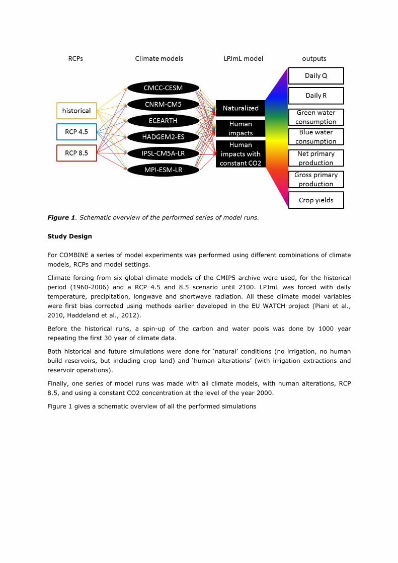
Figure 1. Schematic overview of the performed series of model runs. Study Design For COMBINE a series of model experiments was performed using different combinations of climate models, RCPs and model settings.

Climate forcing from six global climate models of the CMIP5 archive were used, for the historical period (1960-2006) and a RCP 4.5 and 8.5 scenario until 2100. LPJmL was forced with daily temperature, precipitation, longwave and shortwave radiation. All these climate model variables were first bias corrected using methods earlier developed in the EU WATCH project (Piani et al., 2010, Haddeland et al., 2012).

Before the historical runs, a spin-up of the carbon and water pools was done by 1000 year repeating the first 30 year of climate data.

Both historical and future simulations were done for ‘natural’ conditions (no irrigation, no human build reservoirs, but including crop land) and ‘human alterations’ (with irrigation extractions and reservoir operations).

Finally, one series of model runs was made with all climate models, with human alterations, RCP 8.5, and using a constant CO2 concentration at the level of the year 2000.

Figure 1 gives a schematic overview of all the performed simulations

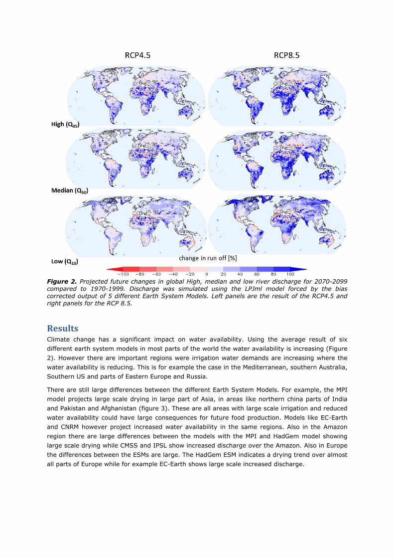
Figure 2. Projected future changes in global High, median and low river discharge for 2070-2099 compared to 1970-1999. Discharge was simulated using the LPJml model forced by the bias corrected output of 5 different Earth System Models. Left panels are the result of the RCP4.5 and right panels for the RCP 8.5.

Results  Climate change has a significant impact on water availability. Using the average result of six different earth system models in most parts of the world the water availability is increasing (Figure 2). However there are important regions were irrigation water demands are increasing where the water availability is reducing. This is for example the case in the Mediterranean, southern Australia, Southern US and parts of Eastern Europe and Russia.

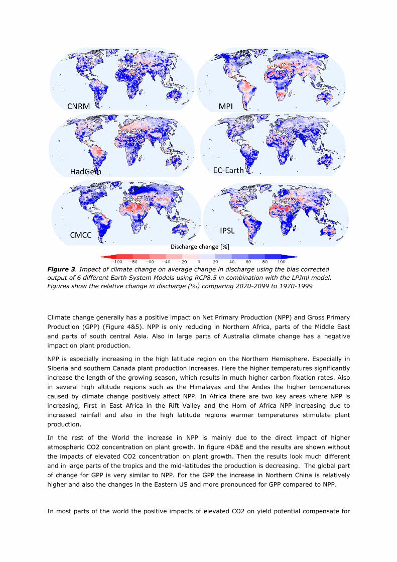
There are still large differences between the different Earth System Models. For example, the MPI model projects large scale drying in large part of Asia, in areas like northern china parts of India and Pakistan and Afghanistan (figure 3). These are all areas with large scale irrigation and reduced water availability could have large consequences for future food production. Models like EC-Earth and CNRM however project increased water availability in the same regions. Also in the Amazon region there are large differences between the models with the MPI and HadGem model showing large scale drying while CMSS and IPSL show increased discharge over the Amazon. Also in Europe the differences between the ESMs are large. The HadGem ESM indicates a drying trend over almost all parts of Europe while for example EC-Earth shows large scale increased discharge.

Figure 3. Impact of climate change on average change in discharge using the bias corrected output of 6 different Earth System Models using RCP8.5 in combination with the LPJml model. Figures show the relative change in discharge (%) comparing 2070-2099 to 1970-1999

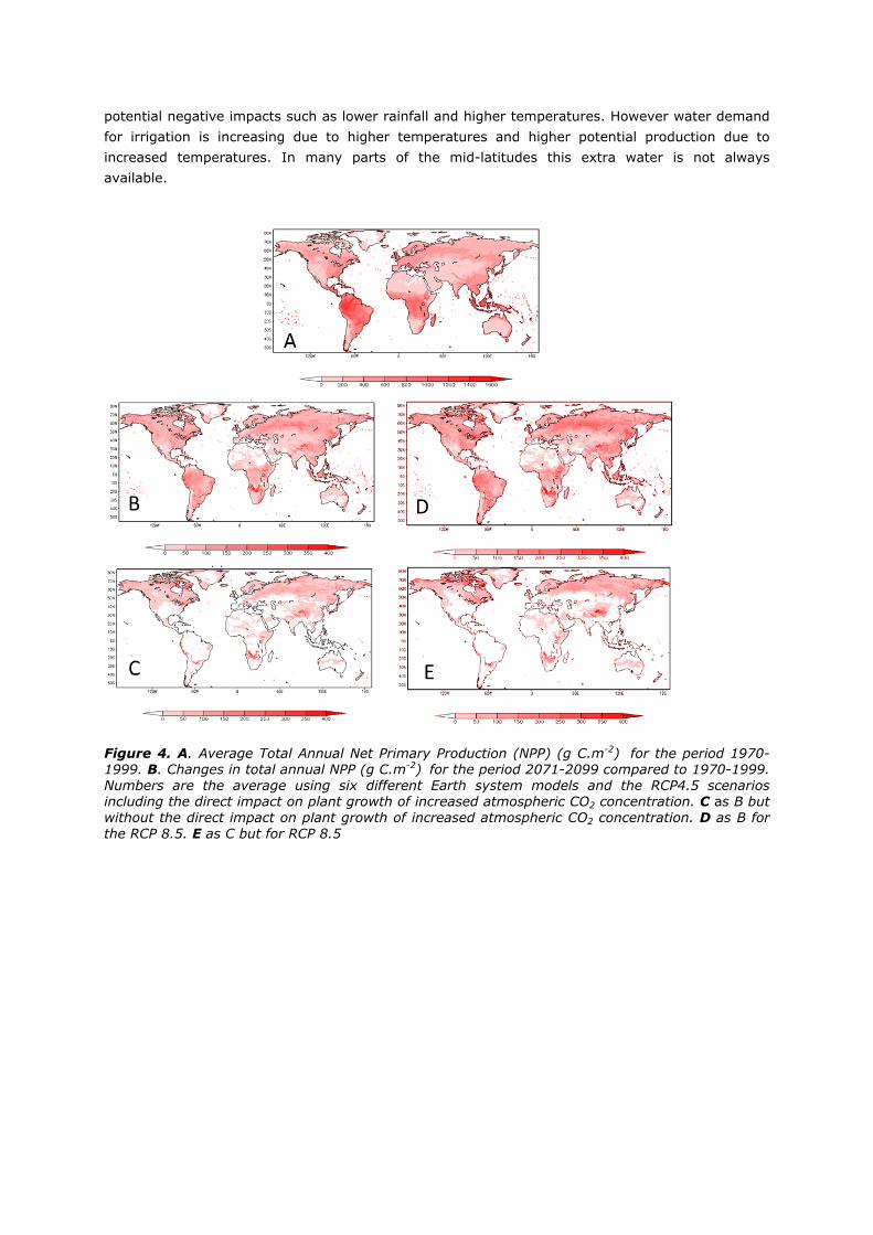
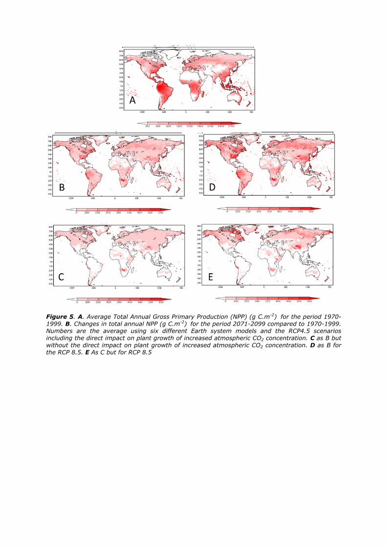
Climate change generally has a positive impact on Net Primary Production (NPP) and Gross Primary Production (GPP) (Figure 4&5). NPP is only reducing in Northern Africa, parts of the Middle East and parts of south central Asia. Also in large parts of Australia climate change has a negative impact on plant production.

NPP is especially increasing in the high latitude region on the Northern Hemisphere. Especially in Siberia and southern Canada plant production increases. Here the higher temperatures significantly increase the length of the growing season, which results in much higher carbon fixation rates. Also in several high altitude regions such as the Himalayas and the Andes the higher temperatures caused by climate change positively affect NPP. In Africa there are two key areas where NPP is increasing, First in East Africa in the Rift Valley and the Horn of Africa NPP increasing due to increased rainfall and also in the high latitude regions warmer temperatures stimulate plant production.

In the rest of the World the increase in NPP is mainly due to the direct impact of higher atmospheric CO2 concentration on plant growth. In figure 4D&E and the results are shown without the impacts of elevated CO2 concentration on plant growth. Then the results look much different and in large parts of the tropics and the mid-latitudes the production is decreasing. The global part of change for GPP is very similar to NPP. For the GPP the increase in Northern China is relatively higher and also the changes in the Eastern US and more pronounced for GPP compared to NPP.

In most parts of the world the positive impacts of elevated CO2 on yield potential compensate for

potential negative impacts such as lower rainfall and higher temperatures. However water demand for irrigation is increasing due to higher temperatures and higher potential production due to increased temperatures. In many parts of the mid-latitudes this extra water is not always available.

Figure 4. A. Average Total Annual Net Primary Production (NPP) (g C.m-2) for the period 1970-1999. B. Changes in total annual NPP (g C.m-2) for the period 2071-2099 compared to 1970-1999. Numbers are the average using six different Earth system models and the RCP4.5 scenarios including the direct impact on plant growth of increased atmospheric CO2 concentration. C as B but without the direct impact on plant growth of increased atmospheric CO2 concentration. D as B for the RCP 8.5. E as C but for RCP 8.5

Figure 5. A. Average Total Annual Gross Primary Production (NPP) (g C.m-2) for the period 1970-1999. B. Changes in total annual NPP (g C.m-2) for the period 2071-2099 compared to 1970-1999. Numbers are the average using six different Earth system models and the RCP4.5 scenarios including the direct impact on plant growth of increased atmospheric CO2 concentration. C as B but without the direct impact on plant growth of increased atmospheric CO2 concentration. D as B for the RCP 8.5. E As C but for RCP 8.5

 

Discussion  and  Conclusion  

Climate change has a large impact on future changes on water and food resources. At global scale climate change increases the water availability and plant production. This is especially the case in the northern parts of the northern hemisphere. Both CO2 concentration and temperatures are important constraints to plant production. Both these factors will increase in future and as a result the potential plant production will increase.

However It is important to note that the modelling framework used here does not include nutrients. So the changes in plant production reported here does not include the impact of nutrient limitations. The actual the responses of climate change however also depend on nutrient availability. Without sufficient nutrient availability CO2 enrichment will not result in much higher plant production. So to ensure that agricultural production will increase in the future improved nutrient management is necessary. To capitalise on the beneficial impacts of climate change it is important to improve the agricultural management strategies (Ludwig and Asseng 2006).

Another important factor affecting plant production is water availability. Climate change affects the rainfall and run-off processes and therefor affects both the ground and surface water avaiability . In large parts of the world, the water availability is increasing which could potentially have a positive impact on agricultural production. However there are also important regions in the world which could face reduced water availability. In several regions such as the Mediterranean and southern Australia water availability is already limiting agriculture. In these regions the potential for agriculture will reduce. The future changes in the hydrological cycle however remain highly uncertain and there are large differences between different Earth System models. This severely complicates the development of adaptation strategies.

It is also important to note that the current analyses focusses on changes in average plant production. Climate change also affects climate variability result in more temperature and rainfall extremes (see deliverable 8.2). The changes in climate variability also increase variability in plant production. This affects ecosystem stability and the reliability of agricultural production. At smaller scales this can affect especially self-subsistence farmers and at larges scales this impacts regional food security.

In conclusion our analyses shows that plant production will be impacted by future climate change. Especially in the high latitude regions plant production will increase. In the semi-arid region around the mid-latitudes plant production is more likely to reduce. However there are still large uncertainties in potential climate change impacts. The two most important uncertainties are firstly, to what extent CO2 concentrations will increase plant production and secondly, the impacts of global warming on the hydrological cycle.

 

References  Amthor J. S. (2001) Effects of atmospheric CO2 concentration on wheat yield: review of results from experiments using various approaches to control CO2 concentration. Field Crops Research 73, 1-34.

Asseng S., Ludwig F., Milroy S., Travasso M. I., Cao W., White J. W. & Wang E. (2009) A Simulation Analysis on Climate Change—Threats or Opportunities for Agriculture

Crop Modeling and Decision Support. pp. 277-81. Springer Berlin Heidelberg.

Biemans H. (2012) Water constraints on future food production. Wageningen Universityq.

Biemans H., Haddeland I., Kabat P., Ludwig F., Hutjes R. W. A., Heinke J., von Bloh W. & Gerten D. (2011) Impact of reservoirs on river discharge and irrigation water supply during the 20th century. Water Resources Research 47.

Biemans H., Hutjes R. W. A., Kabat P., Strengers B. J., Gerten D. & Rost S. (2009) Effects of Precipitation Uncertainty on Discharge Calculations for Main River Basins. Journal of Hydrometeorology 10, 1011-25.

Bondeau A., Smith P. C., Zaehle S., Schaphoff S., Lucht W., Cramer W. & Gerten D. (2007) Modelling the role of agriculture for the 20th century global terrestrial carbon balance. Global Change Biology 13, 679-706.

Drake B. G., Gonzalezmeler M. A. & Long S. P. (1997) More Efficient Plants: a Consequence of Rising Atmospheric Co2? Annual Review of Plant Physiology and Plant Molecular Biology 48, 609-39.

Fader M., Rost S., Muller C., Bondeau A. & Gerten D. (2009) Virtual water content of temperate cereals and maize: Present and potential future patterns. Journal of Hydrology 384, 218-31.

Garcia R. L., Long S. P., Wall G. W., Osborne C. P., Kimball B. A., Nie G. Y., Pinter P. J., Lamorte R. L. & Wechsung F. (1998) Photosynthesis and Conductance of Spring-Wheat Leaves: Field Response to Continuous Free-Air Atmospheric Co2 Enrichment. Plant Cell and Environment 21, 659-69.

Gerten D., Schaphoff S., Haberlandt U., Lucht W. & Sitch S. (2004) Terrestrial vegetation and water balance - hydrological evaluation of a dynamic global vegetation model. Journal of Hydrology 286, 249-70.

Haddeland I., Clark D. B., Franssen W., Ludwig F., Voss F., Arnell N. W., Bertrand N., Best M., Folwell S., Gerten D., Gomes S., Gosling S. N., Hagemann S., Hanasaki N., Harding R., Heinke J., Kabat P., Koirala S., Oki T., Polcher J., Stacke T., Viterbo P., Weedon G. P. & Yeh P. (2011) Multimodel Estimate of the Global Terrestrial Water Balance: Setup and First Results. Journal of Hydrometeorology 12, 869-84.

Haddeland I., Heinke J., Voß F., Eisner S., Chen C., Hagemann S. & Ludwig F. (2012) Effects of climate model radiation, humidity and wind estimates on hydrological simulations. Hydrol. Earth Syst. Sci 16, 305-18.

Kimball B. A., Morris C. F., Pinter P. J., Wall G. W., Hunsaker D. J., Adamsen F. J., Lamorte R. L., Leavitt S. W., Thompson T. L., Matthias A. D. & Brooks T. J. (2001) Elevated Co2, Drought and Soil Nitrogen Effects on Wheat Grain Quality. New Phytologist 150, 295-303.

Lawlor D. W. & Mitchell R. A. C. (2000) Crop ecosystems reponses to climatic change: wheat. In:

Climate change and global crop productivity (eds K. R. Reddy and H. F. Hodges) pp. 57-80. CAB International, Cambridge.

Long S. P., Ainsworth E. A., Rogers A. & Ort D. R. (2004) Rising Atmospheric Carbon Dioxide: Plants Face the Future. Annual Review of Plant Biology 55, 591-628.

Ludwig F. & Asseng S. (2006) Climate change impacts on wheat production in a Mediterranean environment in Western Australia. Agricultural Systems 90, 159-79.

Morison J. I. L. (1985) Sensitivity of stomata and water-use efficiency to high CO2. Plant Cell and Environment 8, 467-74.

Moss R. H., Edmonds J. A., Hibbard K. A., Manning M. R., Rose S. K., van Vuuren D. P., Carter T. R., Emori S., Kainuma M., Kram T., Meehl G. A., Mitchell J. F. B., Nakicenovic N., Riahi K., Smith S. J., Stouffer R. J., Thomson A. M., Weyant J. P. & Wilbanks T. J. (2010) The next generation of scenarios for climate change research and assessment. Nature 463, 747-56.

Peng S. B., Huang J. L., Sheehy J. E., Laza R. C., Visperas R. M., Zhong X. H., Centeno G. S., Khush G. S. & Cassman K. G. (2004) Rice yields decline with higher night temperature from global warming. Proceedings of the National Academy of Sciences of the United States of America 101, 9971-5.

Piani C., Haerter J. & Coppola E. (2010) Statistical bias correction for daily precipitation in regional climate models over Europe. Theoretical and Applied Climatology 99, 187-92.

Rogers G. S., Milham P. J., Gillings M. & Conroy J. P. (1996) Sink Strength May Be the Key to Growth and Nitrogen Responses in N-Deficient Wheat at Elevated Co2. Australian Journal of Plant Physiology 23, 253-64.

Rohwer J., Gerten D. & Lucht W. (2007) Development of funtional irrigation types for improved global crop modelling. Postdam Intstitute for Climate Impact Research, Postdam.

Rost S., Gerten D., Bondeau A., Lucht W., Rohwer J. & Schaphoff S. (2008) Agricultural green and blue water consumption and its influence on the global water system. Water Resources Research 44, W09405.

Sitch S., Smith B., Prentice I. C., Arneth A., Bondeau A., Cramer W., Kaplan J. O., Levis S., Lucht W., Sykes M. T., Thonicke K. & Venevsky S. (2003) Evaluation of ecosystem dynamics, plant geography and terrestrial carbon cycling in the LPJ dynamic global vegetation model. Global Change Biology 9, 161-85.

Wall G. W. (2001) Elevated Atmospheric Co2 Alleviates Drought Stress in Wheat. Agriculture Ecosystems & Environment 87, 261-71.

Weedon G. P., Gomes S., Viterbo P., Shuttleworth W. J., Blyth E., Österle H., Adam J. C., Bellouin N., Boucher O. & Best M. (2011) Creation of the WATCH Forcing Data and Its Use to Assess Global and Regional Reference Crop Evaporation over Land during the Twentieth Century. Journal of Hydrometeorology 12, 823-48.