IMPLEMENTATION CONSIDERATION OF M2M4 SINR ESTIMATION...

DEPARTMENT OF COMMUNICATION ENGINEERING DEGREE PROGRAMME IN WIRELESS COMMUNICATION

IMPLEMENTATION CONSIDERATION OF

M2M4 SINR ESTIMATION ALGORITHM

Author ___________________________________

Nouman Bashir

Supervisor ___________________________________

Matti Latva-aho

Accepted _______/_______2016

Grade ___________________________________

Bashir N. (2016) Implementation consideration of M2M4 SINR estimation

algorithm. University of Oulu, Department of Electrical and Information Engineering.

Master’s Thesis, 50 p.

ABSTRACT

Efficient use of wireless spectrum is needed, due to enormous increase in wireless

devices during last few years. In this context lot of effort is being done to make an

intelligent and cognitive radio system, which can use the spectrum

opportunistically. The ratio of the signal average power to the interference plus

noise average power is called signal to interference plus noise ratio (SINR). SINR

is one of the important parameters that can help in developing cognitive radio

systems, because on the basis of its calculation the spectrum can be utilized

efficiently.

The principle goal of this thesis is to implement a SINR estimation algorithm

for a cognitive radio network (CRN) test-bed. The proposed SINR estimation

algorithm is second order moment and fourth order moment (M2M4) SINR

estimation algorithm, where M2 and M4 are the second order moment and fourth

order moments respectively. The M2M4 estimation algorithm is one of the non-

data-aided (NDA) estimation algorithms. Hence, the algorithm takes the received

signal as input and calculates the second and fourth moments blindly. The

average signal power and average interference plus noise power can be calculated

from these second and fourth order moments, their ratio yields the SINR. The

M2M4 estimation algorithm is first simulated in MATLAB, and then it is

designed for system generator model to draw fair comparison between

simulations and system generator model. The experimental evaluation revealed

that despite of the word length constraint in the system generator model, it

performs reasonably well when compared to the ideal (MATLAB) solution.

The M2M4 estimation algorithm is tested and verified by different test cases,

to ensure its validity. The algorithm is tested for different signal strengths. The

result shows M2M4 is an efficient algorithm for the SINR estimation. However,

the proposed architecture could not fit into the aimed hardware because of heavy

design since it consume more resources than available.

Key words: SINR, estimation algorithms, M2M4, WARP, FPGA

TABLE OF CONTENTS

ABSTRACT

TABLE OF CONTENTS

PREFACE

LIST OF SYMBOLS AND ABBREVIATIONS

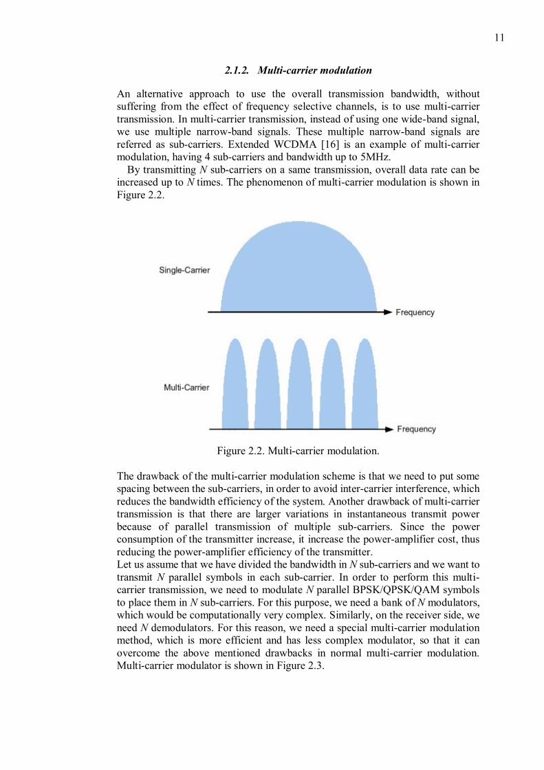
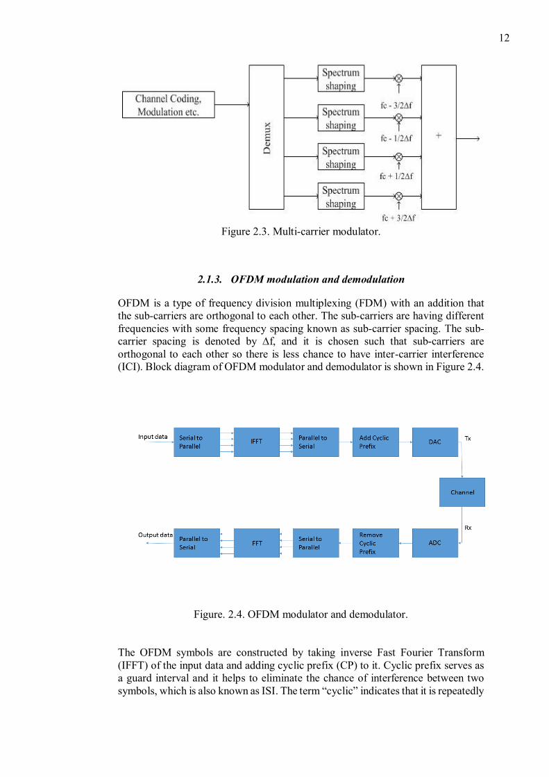
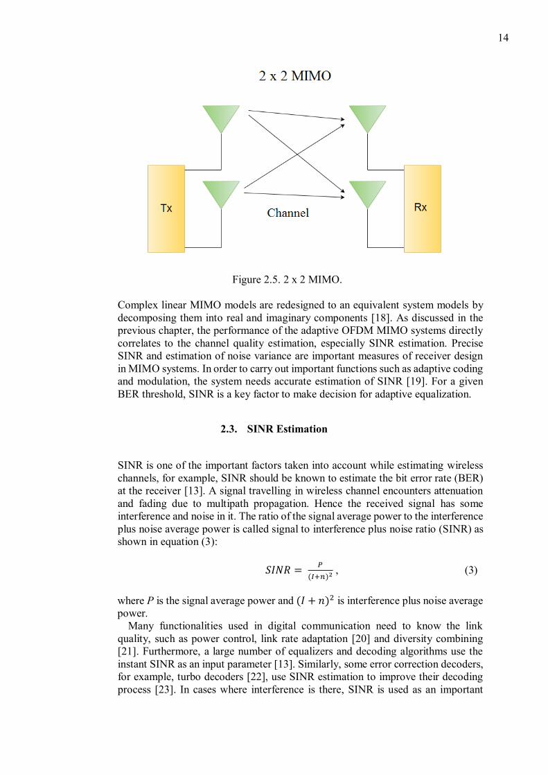
1. INTRODUCTION ............................................................................................ 7 2. SYSTEM MODEL ......................................................................................... 10

2.1. OFDM ................................................................................................ 10 2.1.1. Limitations in single-carrier modulation ................................. 10

2.1.2. Multi-carrier modulation ........................................................ 11 2.1.3. OFDM modulation and demodulation..................................... 12

2.2. MIMO ................................................................................................ 13 2.3. SINR Estimation ................................................................................. 14

2.3.1. Cramer Rao bound.................................................................. 18 2.4. Operation of the estimation algorithm ................................................. 22

3. IMPLEMENTATION PLATFORM ............................................................... 23 3.1. Hardware ............................................................................................ 23

3.1.1. FPGA board ........................................................................... 23 3.1.2. Radio board ............................................................................ 24

3.1.3. Clock Board ........................................................................... 26 3.2. OFDM Reference Design .................................................................... 27

3.2.1. Structure of OFDM reference design ...................................... 27 3.2.2. Training signal ....................................................................... 28

3.2.3. IP cores .................................................................................. 29 3.2.4. MIMO OFDM core ................................................................ 30

3.2.5. Xilinx tools............................................................................. 30 4. IMPLEMENTATION OF M2M4 ALGORITHM ........................................... 32

4.1. Design Consideration .......................................................................... 32 4.2. System Generator modelling ............................................................... 33

4.2.1. Word-length and binary point ................................................. 39 4.2.2. Introduction to CORDIC ........................................................ 40

4.3. Performance Verification .................................................................... 40 5. DISCUSSION ................................................................................................ 44

6. SUMMARY ................................................................................................... 45 7. REFERENCES ............................................................................................... 46

PREFACE

The work presented in this thesis was done for Cognitive Radio Trial Environment

(CORE) project at Centre for Wireless Communication (CWC), University of Oulu.

The aim of the thesis was to design an efficient SINR estimation algorithm, named

M2M4, and implement it on wireless open access research platform (WARP)

hardware.

I would like to thank my supervisor Prof. Matti Latva-aho for all his help and

guidance. Furthermore, I would also like to thank Harri Saarnisaari and Markku

Jokinen for their comments and guidance at every step of my thesis. I would also like

to thank WARP team members for their support and friendly work environment during

the thesis work. I would also like to thank all my friends specially Shahriar

Shahabuddin, Hassan Malik, Saad Saud, Irtiza Hassan and Ijaz Ahmad for their

support during my thesis writing. Finally, I would like to dedicate this thesis work to

all my family members for their love and support along the way.

Oulu, 04 May 2016.

Nouman Bashir

LIST OF SYMBOLS AND ABBREVIATIONS

Nsym Number of Symbols

Nss Number of samples per symbol

𝑥𝛾 Discrete time sampled baseband signal

𝑒𝛾 Discrete time sampled signal

𝑛𝛾 Discrete time sampled noise signal

휀 Expectation value

T Sampling time

3G 3rd Generation of mobile communications

ADC Analog to Digital Converter

AGC Automatic Gain Control

AWGN Additive White Gaussian Noise

BER Bit Error Rate

BRAM Block Random Access Memory

BS Base Station

CE Cognitive Engine

CIR Channel Impulse Response

CMC Center for Multimedia Communication

CORE COgnitive Radio trial Environment

CORDIC Coordinate Rotational Digital Computer

CP Cyclic Prefix

CR Cognitive Radio

CRB Cramer-Rao Bound

CRN Cognitive Radio Network

CSMA/CD Carrier Sense Multiple Access/Collision Detection

CWC Center for Wireless Communication

DA Data Aided

DAC Digital to Analog Converter

dB Decibel

dBm Decibel (milliwatt)

DSP Digital Signal Processing

ED Eigenvalue Decomposition

FCC Federal Communication Commission

FDM Frequency Division Multiplexing

FFT Fast Fourier Transform

FM Frequency Modulation

FPGA Field Programmable Gate Array

GHz Giga-Hertz

I/O Input/Output

I/Q In-phase/Quadrature

ISI Inter-Symbol Interference

ISM Industrial Scientific and Medical

LTE Long Term Evolution

LTE-A Long Term Evolution Advanced

M2M4 Second order Moment and Fourth order Moment

MAC Medium Access Control

MF Matched Filter

MHz Mega-Hertz

MIMO Multiple Input Multiple Output

ML Maximum Likelihood

MPSK M-Array Phase Shift Keying

NDA Non Data Aided

OFDM Orthogonal Frequency Division Multiplexing

PDF Probability Density Function

PLB Processor Local Bus

PM Phase Modulation

PowerPC Power Performance Computing

QoS Quality of Service

RF Radio Frequency

RSSI Received Signal Strength Indicator

RTT Round Trip Time

Rx Receive

SINR Signal to Interference plus Noise Ratio

SNR Signal to Noise Ratio

SNV Squared signal to Noise Variance

SRAM Static Random Access Memory

SSME Split Symbol Moment Estimator

SVR Signal to Variation Ratio

TV Tele-Vision

Tx Transmit

UE User Equipment

UHF Ultra High Frequency

UMTS Universal Mobile Telecommunication System

US United States

WARP Wireless open Access Research Platform

WSS Wide Sense Stationary

1. INTRODUCTION

Number of wireless devices has been increased dramatically during last couple of

years, and with the passage of time this increment is expected to be enormous due

to the fact that everything is going wireless. Modern wireless communication

systems are needed because of increase in number of applications, from the

traditional voice applications to multimedia applications, thus increasing the need

for higher data rate and faster transmission speed. The increase in wireless devices

also results in the problem of scarce spectrum availability.

While travelling in the wireless channel, the signal also suffers rapid fluctuation

in amplitude and phase, which could be due to different reasons, e.g., reflection,

diffraction etc. Due to this reason the transmitted signal might reach at the receiver

over many different paths. This phenomenon is called multipath propagation. These

multipath components of the signal cause fluctuations in the channel. These

fluctuations result in constructive or destructive interference, which is termed as

multipath fading. If either of the transmitter or receiver is moving, then the fading

effect will be time varying. In addition to the fading, other factors which distort the

signal are noise and interference.

Since the signal is propagated in wireless channels, ideally it is necessary to avoid

the fading effects and inter symbol interference (ISI) to maintain the throughput,

but in real life scenario it is rather difficult to do it. ISI is an unwanted phenomenon

in which one symbol gets interference from the subsequent symbols, thus making

the communication less reliable. A multicarrier modulation scheme can be used to

counter the frequency selective fading e.g. orthogonal frequency division

multiplexing (OFDM), which also provides resistance towards ISI [1]. In addition

to this, multiple antenna systems, multiple input multiple output (MIMO) are used,

i.e., spatial multiplexing, to increase the link capacity. A brief description of

multicarrier OFDM and MIMO systems is given in next chapter.

There is a need to design intelligent radio systems which can adapt the changes

in wireless channels. Wireless and mobile devices also have limited capabilities,

e.g., processing power, battery life and transmission range. Hence an intelligent

radio system is needed so that limited resources can be utilized efficiently. A lot of

research has been done, in this context, and researchers developed new wireless

radio access technologies, like Universal Mobile Telecommunication System

(UMTS) and Long Term Evolution (LTE). Moreover, some multi-carrier schemes

have been introduced, like OFDM, which are being used by LTE to enhance 3rd

Generation (3G) wireless technology [2].

This enhancement in 3G wireless technology is still not practical enough to

deliver modern services to the mobile users like high speed internet access and

mobile TV [3]. As discussed earlier, one more problem in this scenario is scarce

spectrum availability. The situation of available spectrum is creating problems to

spare bandwidth for long term evolution advanced (LTE-A) [4]. LTE-A is an

enhancement to the LTE communication standard. The solution for scarce spectrum

availability as proposed in [4], [5] is to deploy LTE-A at ultra-high frequency

(UHF) radio band.

However, the problem of scarce spectrum availability might not be addressed

properly because it is not always scarce spectrum availability rather it is inefficient

utility of the spectrum available. Federal Communication Commission (FCC)

carried out a study in USA which shows that most of the allocated spectrums are

under-utilized [6]. In this regard, cognitive radio (CR) is considered to be an

innovative idea and a good solution to the efficient use of spectrum [7]. CR is an

intelligent radio that gathers knowledge from its environment and adjusts its

parameters to utilize the spectrum efficiently and learns from the results obtained

[8]. Cognition cycle is defined in [9] as a cyclic process that observes the

environment, orients itself, plans, decides and acts. Cognition cycle is shown in

Figure 1.1.

Figure 1.1. Cognition cycle.

One of the important functions performed by a CR is gathering the information

from the outside environment like signal to noise ratio (SNR) measurements, round

trip time (RTT), received signal strength indicator (RSSI) etc. and make decisions

according to these parameters and finally achieve spectrum efficiency. Hence,

cognitive radio is enabling flexibility in the networks, so that the networks can be

more robust. It is expected that next generation wireless networks will support

multimedia applications, they have to carry a lot of traffic like video conferencing

and video calls. Therefore, network will be having a strict quality of service (QoS)

requirement. An efficient SINR estimation algorithm is required to fulfill the QoS

requirement, to perform efficient signal detection and link adaptation [10].

Another significant parameter for modern communication systems, for example

LTE, is link adaptation. Link adaptation is the ability to adapt the channel

parameters according to the link quality. In other words link adaptation can be

denoted as matching of modulation, coding and other control parameters according

to the radio link quality information. Due to frequency selective fading, LTE

subcarriers arrive at the receiver with different quality i.e. they vary over time and

frequency. The time varying behavior of frequency selective channels can be

exploited using link adaptation i.e., optimizing the performance of the channel by

selecting the best modulation, coding and rank scheme (MRCS). This performance

optimization is done according to the current channel state and under certain

constraint e.g., bit error rate (BER). Link adaptation is sufficient to mitigate the

frequency selective fading and utilize the maximum available capacity of the time

varying channel.

The performance of adaptive systems depends on the effectiveness of techniques

used in channel quality estimation, particularly SNR estimation [11]. For example,

OFDM systems use SNR estimation for adaptive coding and modulation, turbo

decoding, etc. [12]. Since interference signals are also present in the received signal

in addition to the noise signals, we use the term signal to interference plus noise

ratio (SINR) instead of SNR. SINR is one of the important indicator that defines

the quality of the data transmission [13]. A high SINR estimate gives us the

information that the link quality is good, and vice versa. Hence SINR is considered

to be one of the decisive factors while making decision for link adaptation in a CR.

This thesis is carried out as a part of cognitive radio trial environment (CORE)

project [14]. The principal goal of CORE project was to develop a testing

environment to test cognitive functionalities on different wireless environments.

This research focuses on the implementation of an efficient SINR estimation

algorithm on Wireless open-Access Research Platform (WARP). A SINR

estimation algorithm, named second order moment and fourth order moment

(M2M4) [15], is proposed.

The rest of the thesis is organized sequentially as follows: In chapter 2, different

SINR estimation algorithms are compared and the reason behind choosing the

M2M4 SINR estimation algorithm is discussed. In this chapter, operation of M2M4

estimation algorithm is also explained. Chapter 3 discusses hardware components

of WARP radio platform. Furthermore, chapter 3 also describes about the OFDM

reference design. Implementation of M2M4 SINR estimation algorithm on the

WARP radio platform is explained in chapter 4. In the same chapter, different tools

used during the implementation are also discussed. Additionally, chapter 4 includes

the performance analysis of the proposed SINR estimation algorithm. The

discussion and possible development in the future is presented in chapter 5. Finally,

the whole work is summarized in chapter 6.

10

2. SYSTEM MODEL

In this chapter we discuss the theoretical background of OFDM, MIMO and SINR

estimation. Different SINR estimation algorithms and their performance

comparison is also presented in this chapter.

2.1. OFDM

OFDM is a multi-carrier modulation scheme which uses the spectrum efficiently

because frequency band is divided into many subcarriers that are orthogonal to each

other. In order to understand the multi-carrier modulation, we need to overview the

drawbacks and limitations of single carrier modulation and the reason why multi-

carrier modulation is needed.

2.1.1. Limitations in single-carrier modulation

As discussed in the previous chapter that spectrum bandwidth is a limited resource

and the efficient use of the bandwidth is needed. In order to improve the date rate

in a given bandwidth, higher-order modulation schemes, e.g., quadrature phase shift

keying (QPSK), quadrature amplitude modulation (QAM) and 64-QAM are used.

The use of higher-order modulation scheme enables more information bits to be

transmitted per symbol. The number of bits per symbol are 2, 4 and 6 for QPSK,

16-QAM and 64-QAM respectively. Signal constellations of these modulations

schemes are given in Figure 2.1.

Figure 2.1. Signal constellations for QPSK, 16QAM and 64 QAM.

Since these single-carrier higher-order modulations schemes carry more

information bits, hence they can utilize the bandwidth efficiently by providing high

data rate. However, achieving high data rate require more SNR at the receiver, for

a given bit-error probability. It means 16-QAM and 64-QAM require more SNR at

the receiver, as compared to QPSK. Therefore it is difficult to achieve the high data

rates using single-carrier modulation in frequency selective fading channel. Due to

this limitation, we need to have some multi-carrier modulation scheme which can

perform better in the channels having high frequency selective fading.

11

2.1.2. Multi-carrier modulation

An alternative approach to use the overall transmission bandwidth, without

suffering from the effect of frequency selective channels, is to use multi-carrier

transmission. In multi-carrier transmission, instead of using one wide-band signal,

we use multiple narrow-band signals. These multiple narrow-band signals are

referred as sub-carriers. Extended WCDMA [16] is an example of multi-carrier

modulation, having 4 sub-carriers and bandwidth up to 5MHz.

By transmitting N sub-carriers on a same transmission, overall data rate can be

increased up to N times. The phenomenon of multi-carrier modulation is shown in

Figure 2.2.

Figure 2.2. Multi-carrier modulation.

The drawback of the multi-carrier modulation scheme is that we need to put some

spacing between the sub-carriers, in order to avoid inter-carrier interference, which

reduces the bandwidth efficiency of the system. Another drawback of multi-carrier

transmission is that there are larger variations in instantaneous transmit power

because of parallel transmission of multiple sub-carriers. Since the power

consumption of the transmitter increase, it increase the power-amplifier cost, thus

reducing the power-amplifier efficiency of the transmitter.

Let us assume that we have divided the bandwidth in N sub-carriers and we want to

transmit N parallel symbols in each sub-carrier. In order to perform this multi-

carrier transmission, we need to modulate N parallel BPSK/QPSK/QAM symbols

to place them in N sub-carriers. For this purpose, we need a bank of N modulators,

which would be computationally very complex. Similarly, on the receiver side, we

need N demodulators. For this reason, we need a special multi-carrier modulation

method, which is more efficient and has less complex modulator, so that it can

overcome the above mentioned drawbacks in normal multi-carrier modulation.

Multi-carrier modulator is shown in Figure 2.3.

12

Figure 2.3. Multi-carrier modulator.

2.1.3. OFDM modulation and demodulation

OFDM is a type of frequency division multiplexing (FDM) with an addition that

the sub-carriers are orthogonal to each other. The sub-carriers are having different

frequencies with some frequency spacing known as sub-carrier spacing. The sub-

carrier spacing is denoted by ∆f, and it is chosen such that sub-carriers are

orthogonal to each other so there is less chance to have inter-carrier interference

(ICI). Block diagram of OFDM modulator and demodulator is shown in Figure 2.4.

Figure. 2.4. OFDM modulator and demodulator.

The OFDM symbols are constructed by taking inverse Fast Fourier Transform

(IFFT) of the input data and adding cyclic prefix (CP) to it. Cyclic prefix serves as

a guard interval and it helps to eliminate the chance of interference between two

symbols, which is also known as ISI. The term “cyclic” indicates that it is repeatedly

13

prefixed after each symbol. The CP is efficient if its minimum length is equal to the

duration of channel impulse response (CIR). Baum et al. [17] describe that CP

shorter than the CIR effects in degradation of OFDM signal. He also explained that

the longer CP makes OFDM system more robust to timing errors.

There are several benefits of OFDM, one of them is that it utilizes the spectrum

efficiently by using large number of overlapping sub-carriers. Moreover it is robust

to frequency selective channels as compared to single carrier systems. As discussed

earlier, use of CP helps to eliminate the chance of ISI. Use of Fast Fourier

Transform (FFT) for modulation and demodulation makes its computational

efficiency better as compared to other techniques.

2.2. MIMO

In order to improve system capacity as discussed earlier, we can use several

antennas instead of single antenna for transmission and/or reception. This kind of

architecture is called MIMO system. The benefit of MIMO is that array gain, spatial

multiplexing and diversity gain jointly increases the system capacity. Therefore,

increasing the data throughput without additional bandwidth yields spectral

efficiency. Additionally, the capacity growth in MIMO is linear such that 2x2

MIMO doubles and 4x4 MIMO quadruples the capacity. MIMO system capabilities

are further illuminated by the fact that they are part of communication standards

like LTE, IEEE 802.16e and IEEE 802.11n [16].

Despite having a widespread application, the equipment cost of the MIMO

systems are high because of the multiple antennas used. Due to the same reason,

the complexity and the computational overhead of multi-dimensional signal

processing could surge.

Imagine a MIMO system having N number of antennas at the transmitter and M

number of antennas at the receiver such that N ≥ M. The signal received can be

represented mathematically as explained in equation (1):

𝑦𝑠 = 𝐻𝑠𝑥𝑠 + 𝑛𝑠 (1)

Where 𝐻𝑠 is channel matrix, 𝑥𝑠 is the transmitted signal, 𝑛𝑠 is the white Gaussian

noise and 𝑠 is referred to as the number of subcarriers. The noise vector 𝑛𝑠 is

independent and has complex zero mean. The channel matrix contains channel

coefficients ℎ𝑛,𝑚 where 𝑛 is the transmitting antenna and 𝑚 is receiving antenna.

The channel matrix can be expressed in equation (2) as:

𝐻𝑠 = (

ℎ1,1 ⋯ ℎ1,𝑁

⋮ ⋱ ⋮ℎ𝑀,1 ⋯ ℎ𝑀,𝑁

) (2)

14

Figure 2.5. 2 x 2 MIMO.

Complex linear MIMO models are redesigned to an equivalent system models by

decomposing them into real and imaginary components [18]. As discussed in the

previous chapter, the performance of the adaptive OFDM MIMO systems directly

correlates to the channel quality estimation, especially SINR estimation. Precise

SINR and estimation of noise variance are important measures of receiver design

in MIMO systems. In order to carry out important functions such as adaptive coding

and modulation, the system needs accurate estimation of SINR [19]. For a given

BER threshold, SINR is a key factor to make decision for adaptive equalization.

2.3. SINR Estimation

SINR is one of the important factors taken into account while estimating wireless

channels, for example, SINR should be known to estimate the bit error rate (BER)

at the receiver [13]. A signal travelling in wireless channel encounters attenuation

and fading due to multipath propagation. Hence the received signal has some

interference and noise in it. The ratio of the signal average power to the interference

plus noise average power is called signal to interference plus noise ratio (SINR) as

shown in equation (3):

𝑆𝐼𝑁𝑅 = 𝑃

(𝐼+𝑛)2 , (3)

where P is the signal average power and (𝐼 + 𝑛)2 is interference plus noise average

power.

Many functionalities used in digital communication need to know the link

quality, such as power control, link rate adaptation [20] and diversity combining

[21]. Furthermore, a large number of equalizers and decoding algorithms use the

instant SINR as an input parameter [13]. Similarly, some error correction decoders,

for example, turbo decoders [22], use SINR estimation to improve their decoding

process [23]. In cases where interference is there, SINR is used as an important

15

measure to determine link quality [24]. In multiuser wireless communication, SINR

holds a critical role in decision making for resource allocation at physical layer and

higher layers. The importance of SINR estimation is because of the fact that

numbers of wireless devices have been increased rapidly during past few years and

they cause interference in the spectrum [25].

Depending upon the amount of information available in the received signal,

SINR estimators are usually categorized into two types: data-aided (DA) and non-

data-aided (NDA) estimators. DA estimators work on the basis on known

transmitted data, also called pilots. DA estimators are further classified into two

types; TxDA and RxDA. DA estimator which needs the exact information from

transmitted sequence is termed as TxDA, and the DA estimator which uses the

estimate of transmitted sequence from receiver itself is called RxDA. While the

NDA estimators derive solely from the unknown information, or from the

information present in the received signal. NDA estimation is also termed as blind

estimation. DA estimators might have better performance but they have one

drawback, training symbols insertion might affect the throughput [26]. In [26],

Haifeng investigated the performance of different NDA estimation techniques.

During past few decades, lots of different SINR estimation techniques have been

developed. In [27], Pauluzzi and Beaulieu gave a comparison of different SINR

estimation algorithms. We discuss these estimation algorithms one by one:

1. The Split-Symbol Moment Estimator (SSME) [28] by Shah and Hinedi. The

working of SSME is based on the fact that the signals, having required information,

are correlated in the same symbol interval while the noise signals remain

uncorrelated. The SSME takes the received signal (yij) as input which is sum of

filtered signal (sij) and noise samples (nij):

𝑦𝑖𝑗 = 𝑠𝑖𝑗 + 𝑛𝑖𝑗 . (4)

The received signal symbols are divided into two halves Yαj and Yβj as:

𝑌𝛼𝑗 = ∑ 𝑦𝑖𝑗

(𝑁𝑠2

)−1

𝑖=0, (5)

𝑌𝛽𝑗 = ∑ 𝑦𝑖𝑗(𝑁𝑠−1)

𝑖=𝑁𝑠/2 . (6)

These two halves are summed and squared which gives Xssj, refer to equation (7):

𝑋𝑠𝑠𝑗 = (𝑌𝛼𝑗 + 𝑌𝛽𝑗)2. (7)

Then these two halves are multiplied which yields Xpj as depicted in equation (8):

𝑋𝑝𝑗 = 𝑌𝛽𝑗 . 𝑌𝛼𝑗. (8)

If the noise samples at the input are uncorrelated, then Xssj would be an estimate of

total power and Xpj would be an estimate to signal power, on per symbol basis.

These estimates are made better by averaging over n symbols, yielding mss and mp,

shown in equation (9) and (10):

𝑚𝑠𝑠 = 1/𝑛 ∑ 𝑋𝑠𝑠𝑗𝑛𝑗=1 , (9)

16

𝑚𝑝 = 1/𝑛 ∑ 𝑋𝑝𝑗𝑛𝑗=1 . (10)

Finally, mp is weighted and subtracted from mss to get estimate of noise power,

which is the used to estimate the SNR, as in equation (11):

𝑆𝑁𝑅∗ = 𝑚𝑝

2 (1

4𝑚𝑠𝑠−𝑚𝑝)

. (11)

2. Maximum Likelihood (ML) estimator [29] by Gagliardi and Thomas. It works

by converting the SINR estimation problem into classical ML estimation of signal’s

amplitude [26].

We considering a complex, discreet, band-limited model of coherent M-ary PSK

symbols in complex AWGN model, the signal received at the receiver can be

represented as:

𝑟𝑘 = √𝑆 𝑚𝑘 + √𝑁 𝑍𝑘, (12)

where 𝑆 is signal power scale factor, 𝑁 is noise power scale factor, 𝑍𝑘 is complex

AWGN with zero mean and 𝑚𝑘 is sampled information signal, which is given as

equation (13):

𝑚𝑘 = ∑ 𝑎𝑛𝑛 ℎ𝑘 − 𝑛𝑁𝑠𝑠, (13)

where ℎ𝑘 represents RRC filter tap coefficients. The above equation can be re-

written in terms of in-phase and quadrature components as in equation (14):

𝑟𝑘 = √𝑆(𝑚𝐼𝑘+ 𝑗𝑚𝑄𝑘

) + √𝑁 (𝑍𝐼𝑘+ 𝑗𝑍𝑄𝑘

). (14)

Let √𝑁 𝑍𝐼𝑘= 𝑉𝐼𝑘

and √𝑁 𝑍𝑄𝑘= 𝑉𝑄𝑘

represent in-phase and quadrature

components of the noise, respectively, each having zero mean and variance 𝑁/2.

We assume that in-phase and quadrature components of noise are independent with

probability density function (PDF) equation (15):

𝑓(𝑉𝐼𝑘, 𝑉𝑄𝑘

) = 1

𝜋𝑁 𝑒−(𝑉𝐼𝑘

2+𝑉𝑄𝑘2) 𝑁⁄

. (15)

The joint PDF of in-phase and quadrature components of received signal sample

can be written as equation (16):

𝑓(𝑟𝐼𝑘, 𝑟𝑄𝑘

|𝑆, 𝑁, 𝑖) = 1

𝜋𝑁 𝑒𝑥𝑝 (

(𝑟𝐼𝑘−√𝑆𝑚𝐼𝑘

(𝑖))2+(𝑟𝑄𝑘−√𝑆𝑚𝑄𝑘

(𝑖))2

𝑁) , (16)

where 𝑚𝐼𝑘

(𝑖) and 𝑚𝑄𝑘

(𝑖) are the real and imaginary parts of above equation, and the

superscript i denotes the ith sequence of 𝑀𝑁𝑠𝑦𝑚possible transmitted message

sequences [27]. We assume that both signal and noise sequences are independent

so their joint PDF is given by equation (17):

𝑓(𝐫𝐈, 𝐫𝐐|𝑆, 𝑁, 𝑖) = ∏ 𝑓(𝑟𝐼𝑘, 𝑟𝑄𝑘

|𝑆, 𝑁, 𝑖)𝐾−1𝑘=0

17

= (𝜋𝑁)−𝐾𝑒𝑥𝑝 [−1

𝑁(∑ (𝑟𝐼𝑘

− √𝑆𝑚𝐼𝑘

(𝑖))2𝐾−1𝑘=0 + ∑ (𝑟𝑄𝑘

− √𝑆𝑚𝑄𝑘

(𝑖))2𝐾−1𝑘=0 )] , (17)

where 𝐫𝐈 is sequence of in-phase components of received signal

{𝑟𝐼0, 𝑟𝐼1

, 𝑟𝐼2, … . , 𝑟𝐼𝑘−1

} and 𝐫𝐐 is sequence of quadrature components of the received

signal {𝑟𝑄0, 𝑟𝑄1

, 𝑟𝑄2, … . , 𝑟𝑄𝑘−1

}. The likelihood function is denoted by Γ and is given

as in equation (18):

Γ(𝑆, 𝑁, 𝑖) = ln 𝑓(𝐫𝐈, 𝐫𝐐|𝑆, 𝑁, 𝑖)

= −𝐾 ln(𝜋𝑁) − 1

𝑁 [(∑ (𝑟𝐼𝑘

− √𝑆𝑚𝐼𝑘

(𝑖))2𝐾−1𝑘=0 + ∑ (𝑟𝑄𝑘

− √𝑆𝑚𝑄𝑘

(𝑖))2𝐾−1𝑘=0 )] , (18)

In order to find the ML estimate of the SNR, we use the property that ML estimate

of the signal and noise is the ratio of ML estimate of signal and noise individually.

Hence ML estimate of SNR can be written as equation (19):

�� = ��𝑀𝐿

��𝑀𝐿 . (19)

The respective solution for ��𝑀𝐿 and ��𝑀𝐿 can be written as equation (20) and (21)

respectively:

��𝑀𝐿 = [1

𝐾∑ (𝑟𝐼𝑘

𝑚𝐼𝑘(��)+𝑟𝑄𝑘

𝑚𝑄𝑘(��))𝐾−1

𝑘=0

1

𝐾∑ [(𝑚𝐼𝑘

(��))2

+(𝑚𝑄𝑘(��))

2]𝐾−1

𝑘=0

]

2

, (20)

��𝑀𝐿 = 1

𝐾 ∑ (𝑟𝐼

2 + 𝑟𝑄2) − ��𝐾−1

𝑘=0 1

𝐾 ∑ [(𝑚𝐼𝑘

(��))2

+ (𝑚𝑄𝑘

(��))2

]𝐾−1𝑘=0 . (21)

3. Squared Signal to Noise Variance (SNV) [30] by Gilchriest. SNV works on the

matched filter (MF) and estimates the noise variance by taking the first moment and

the second moment of the sampled output. The sampled output of MF can be

expressed as equation (22):

[

1

𝑁𝑠𝑦𝑚 ∑ |𝑦𝑛|

𝑁𝑠𝑦𝑚−1

𝑛=0 ]2

1

𝑁𝑠𝑦𝑚−1 ∑ 𝑦𝑛−

1

𝑁𝑠𝑦𝑚(𝑁𝑠𝑦𝑚−1)[ ∑ |𝑦𝑛|

𝑁𝑠𝑦𝑚−1

𝑛=0 ]2𝑁𝑠𝑦𝑚−1

𝑛=0

. (22)

The SNV can be described as special case of ML SNR estimator, however the SNV

works at the optimally sampled output of MF. Whereas, ML operates on the

samples per symbol to the MF input.

4. Signal to Variation Ratio (SVR) estimator, as described by Brandao et al. in

[31], is a moments-based method and can be used to estimate channel quality in

AWGN channels. Originally the estimator was designed for M-ary PSK but in [27]

Pauluzzi et al. derived it for complex channels and showed how to use it for real-

time calculations without waiting for the whole training sequence.

The SVR estimator is a function of parameter β, which is expressed

mathematically by equation (23):

18

𝛽 = 𝐸{𝑦𝑛𝑦𝑛

∗𝑦𝑛−1𝑦𝑛−1∗}

𝐸{(𝑦𝑛𝑦𝑛∗)2}−𝐸{𝑦𝑛𝑦𝑛

∗𝑦𝑛−1𝑦𝑛−1∗}

, (23)

where E is the expectation operator. The term 𝐸{(𝑦𝑛𝑦𝑛∗)2} is the fourth order

moment, which will be explained later in this chapter. Simplifying other term in

equation (24), we get:

𝐸{𝑦𝑛𝑦𝑛∗𝑦𝑛−1𝑦𝑛−1

∗} = 𝑆2 + 2𝑆𝑁 + 𝑁2. (24)

We can write S/N = ρ, substituting it in equation (24) and simplifying the

equation (23) results in:

𝛽 = 𝜌2+2𝜌+1

(𝑘𝑎−1)𝜌2+2𝜌+(𝑘𝑤−1) , (25)

where 𝑘𝑎and 𝑘𝑤 are kurtosis of signal and kurtosis of noise respectively. The

equation (25) can be simplified to compute 𝜌, which is the SNR estimate for

complex channels:

��𝑆𝑉𝑅,𝐶𝑜𝑚𝑝𝑙𝑒𝑥 = (𝛽−1)± √(𝛽−1)2−[1−𝛽(𝑘𝑎−1)][1−𝛽(𝑘𝑤−1)]

1−𝛽(𝑘𝑎−1) . (26)

For real signals, the parameter 𝛽 is expressed mathematically as:

𝛽 = 𝐸{𝑦𝑛

2𝑦𝑛−12}

𝐸{𝑦𝑛4}−𝐸{𝑦𝑛

2𝑦𝑛−12}

. (27)

The term 𝐸{𝑦𝑛4} is fourth order moment, so the equation (27) is simplified same as

we simplified equation (23) and (24), we get the SVR estimator for real channels:

��𝑆𝑉𝑅,𝑅𝑒𝑎𝑙 = (2𝛽−1)± √(2𝛽−1)2−[1−𝛽(𝑘𝑎−1)][1−𝛽(𝑘𝑤−1)]

1−𝛽(𝑘𝑎−1) . (28)

5. Second order moment and fourth order moment (M2M4) [15] by Matzner and

Englberger, M2M4 is a well know estimator and it computes the second and fourth

order moments of the noisy signal. [26]. Detailed working of M2M4 estimator is

discussed in chapter 2.4.

2.3.1. Cramer Rao bound

To analyze the performance of any estimator, Cramer Rao Bound (CRB) is used as

a reference. It is named after two mathematicians Harald Cramer and C.R. Rao.

Cramer Rao bound states that variance of the estimate (𝜃) of any unknown

deterministic parameter (θ) is bounded by the reciprocal of the Fischer

information 𝐼(𝜃). Mathematically, it is written as:

𝑣𝑎𝑟 (𝜃) ≥ 1

𝐼(𝜃) , (29)

where 𝐼(𝜃) is the fisher information, defined as:

19

𝐼(𝜃) = 𝐸 [(𝜕𝑙(𝑥;0)

𝜕𝜃)

2

] (30)

= −𝐸 [𝜕2𝑙(𝑥;0)

𝜕𝜃2] , (31)

where 𝐸 is the expectation and 𝑙(𝑥; 0) is log of likelihood function:

𝑙(𝑥; 0) = log(𝑓(𝑥; 0)) . (32)

In [32] Thomas derived CRB for real channels and based on his derivation

Pauluzzi [27] derived CRB for complex channels and compared the results with

real channels. Mathematical expression for CRB is given by following equation:

[27]

𝑣𝑎𝑟{��} ≥ −(

𝜕

𝜕𝜌 𝐸{��})

2𝐸{

𝜕2Г

𝜕𝑁2}

𝐸{𝜕2Г

𝜕𝜌2}𝐸{𝜕2Г

𝜕𝑁2}−𝐸{𝜕2Г

𝜕𝜌𝜕𝑁}

2 , (33)

where Г is the likelihood function defined in equation (18), here we rewrite it

according to the terms 𝜌 and 𝑁:

Г(𝜌, 𝑁, 𝑖) = ln 𝑓(𝐫𝐈, 𝐫𝐐| 𝜌, 𝑁, 𝑖) (34)

= −𝐾 ln(𝜋𝑁) − 1

𝑁[∑ (𝑟𝐼𝑘

− √𝜌𝑁𝑚𝐼𝑘

(𝑖))2

+𝐾−1𝑘=0

∑ (𝑟𝑄𝑘− √𝜌𝑁𝑚𝑄𝑘

(𝑖))2

𝐾−1𝑘=0 ] . (35)

The expectation of the partial derivatives of the likelihood function from previous

equation:

𝐸 {𝜕2Г

𝜕𝜌2} = −

𝐾

2𝜌𝑁𝑠𝑠 , (36)

𝐸 {𝜕2Г

𝜕𝑁2} = −

𝐾(2+𝜌

𝑁𝑠𝑠⁄ )

2𝑁2 , (37)

𝐸 {𝜕2Г

𝜕𝜌𝜕𝑁} = −

𝐾

2𝑁𝑁𝑠𝑠 . (38)

Substituting the values of partial derivatives in equation (33), we get:

𝑣𝑎𝑟{��} ≥ 2𝜌

𝑁𝑠𝑦𝑚+

𝜌2

𝑁𝑠𝑠𝑁𝑠𝑦𝑚 . (39)

The equation (39) is the required Cramer Rao bound.

20

The graphical comparison of performance of the above mentioned estimation

algorithms, is shown in Figure 2.6 and figure 2.7. We simulated different estimators

using the same training symbols, but in our simulations we used random phase with

training symbols for M2M4 estimator, while with the SVR, SNV, and ML simply

training symbols were used. The similar comparison was also done by Pauluzzi et.al

in [27].

Figure 2.6. SNR estimation comparison.

21

Figure 2.7. MSE of SNR estimation algorithms.

According to the graphical results shown in Figure 2.6 and Figure 2.7, M2M4 SINR

estimation algorithm has better performance as compared to signal-to-variation

ratio (SVR) estimation and squared signal-to-noise variance (SNV), but it is almost

equal to the Cramer-Rao bound (CRB).

Apart from the comparison done by Pauluzzi and Beaulieu, there are some more

estimation algorithms which work on the basis on Eigenvalue decomposition (ED)

[33] [34] and they also do not need any prior information like modulation type or

data rate. In [27], Pauluzzi and Beaulieu concluded that M2M4 is one of best

performance estimation algorithms and that the M2M4 estimation algorithm is

easier to implement, as compared to other SINR estimators. Originally M2M4

estimator was developed for M-ary phase shift keying (MPSK) signals, and can be

used for phase modulation (PM) and frequency modulation (FM) signals. In [23],

Linn mentioned that M2M4 is one of the most widely used SINR estimators. A

hardware implementation of M2M4 estimation algorithm is presented in [35].

Since M2M4 estimator is a blind estimator, i.e., it does not require known

symbols for estimation. It has low computational complexity, so real time

implementation is easy [26]. It has a linear response and doesn’t have any upper

limit for estimation. It is because of these reasons I chose to work on M2M4

estimation algorithm for my thesis work.

22

2.4. Operation of the estimation algorithm

The operation principle of M2M4 estimation algorithm is explained in [13], [15].

The complex baseband signal at the output of the demodulator, if sampled at symbol

rate T, gives the sequence < 𝑥 > as in equation (40).

𝑥𝛾 = 𝑒𝛾 + 𝑛𝛾; 𝑥𝛾 , 𝑒𝛾 , 𝑛𝛾 ∈ 𝐶; ∀𝛾∈ 𝑍 (40)

where 𝛾 is for discrete time index, and 𝑒𝛾 and 𝑛𝛾 are discrete time signal and noise

samples respectively. The sequences < 𝑒 > and < 𝑛 > are assumed to be wide-sense

stationary (WSS) and since they are using Gaussian channel so their probability

density functions (PDF) are known. The aim is to compute average energy of the

signal (휀 {𝑒𝑒∗}) and average energy of the noise (휀{𝑛𝑛∗}) from the sequence of

received signal < 𝑥 > [13].

The second order moment is calculated as equation (41) and (42) respectively,

𝑀2 = 휀 {𝑥𝑥∗} = 휀{ 𝑒𝑒∗ + 𝑛𝑛∗ + 𝑒𝑛∗ + 𝑒∗𝑛 } (41)

𝑀2 = 휀{𝑒𝑒∗} + 휀{𝑛𝑛∗} = 𝑃𝑑 + 𝑃𝑛 (42)

And, fourth order moment is calculated as equation (43).

𝑀4 = 휀{(𝑥𝑥∗)2} = 휀{(𝑒𝑒∗)2} + 휀{(𝑛𝑛∗)2} + 4𝑃𝑑𝑃𝑛 (43)

where 𝑃𝑑 = 휀{𝑒𝑒∗} is the average signal power, 𝑃𝑛 = 휀{𝑛𝑛∗} is the average noise

power and 휀{. } denotes the expectation operator.

By solving (4), the signal average power is computed as equation (44).

𝑃𝑑 = √(2𝑀22 − 𝑀4) (44)

And the interference plus noise average power is computed from (45) as,

𝑃𝑛 = 𝑀2 − 𝑃𝑑 (45)

The required SINR is the ratio of average signal power 𝑃𝑠 and the average

interference plus noise power 𝑃𝑛 as in equation (46).

𝑆𝐼𝑁𝑅 =𝑃𝑑

𝑃𝑛=

√(2𝑀22−𝑀4)

𝑀2− √(2𝑀22−𝑀4)

(46)

23

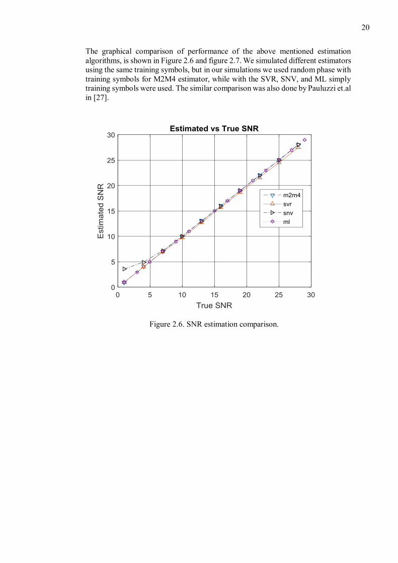
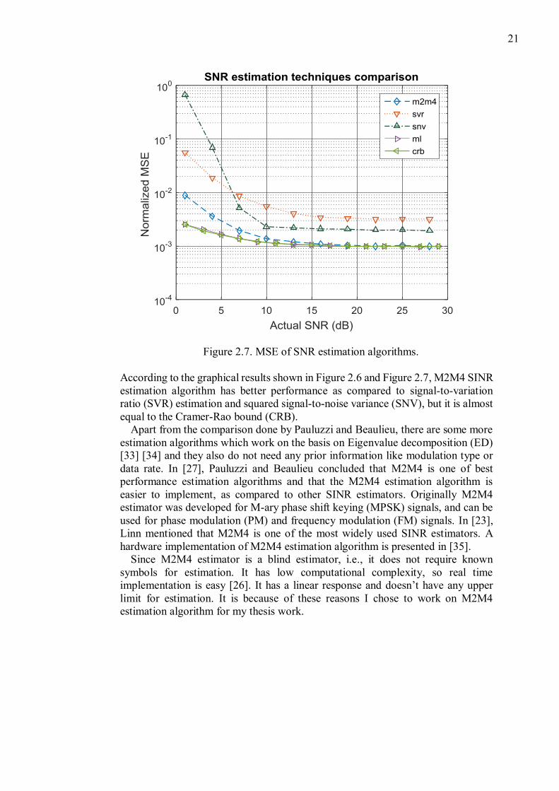
3. IMPLEMENTATION PLATFORM

The implementation platform used in this thesis work is Wireless Open Access

Research Platform (WARP). WARP has been developed by the researchers at

Centre for Multimedia Communication at Rice University USA. WARP platform

is a flexible test platform for wireless systems and it consists of FPGA chip

hardware and a reference design. Since the FPGA hardware is programmable one

can use them for implementation of customized physical layer as well as a MAC

layer and can be used as a prototype for new advanced wireless algorithms [36].

WARP board consists of four auxiliary slots for daughter cards. Two radio boards

are used to implement the real time MIMO scenario. The RF components on the

radio board are supporting 2.4 GHz and 5 GHz ISM channels. Custom I/O boards

can also be used in daughter card slots. Combination of both WARP hardware and

reference design makes a complete OFDM communication system; reference

design controls the hardware.

3.1. Hardware

The WARP board hardware mainly consists of 3 important components which are:

1. FPGA board

2. Radio board

3. Clock board

These hardware boards are described with detail in following:

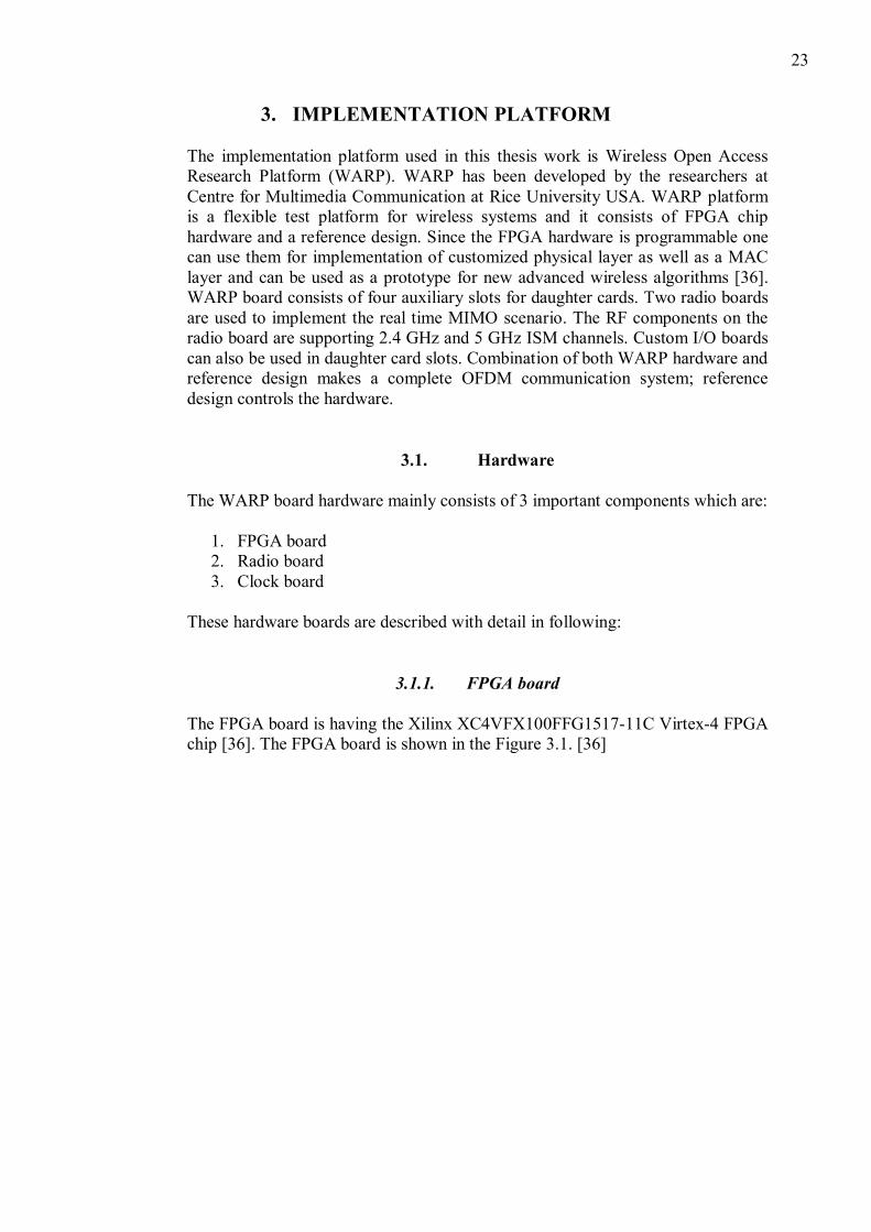
3.1.1. FPGA board

The FPGA board is having the Xilinx XC4VFX100FFG1517-11C Virtex-4 FPGA

chip [36]. The FPGA board is shown in the Figure 3.1. [36]

24

Figure 3.1. WARP FPGA board.

WARP FPGA is designed for intensive DSP operations, for example, parallel

processing of different algorithms. Advanced algorithms can be implemented at

higher layers using the powerPC processor cores which are embedded in this FPGA.

This FPGA has flexibility to connect various peripherals and to create multi-

processor systems [37].

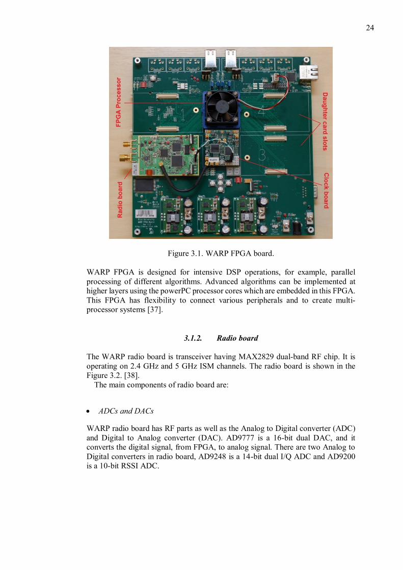
3.1.2. Radio board

The WARP radio board is transceiver having MAX2829 dual-band RF chip. It is

operating on 2.4 GHz and 5 GHz ISM channels. The radio board is shown in the

Figure 3.2. [38].

The main components of radio board are:

ADCs and DACs

WARP radio board has RF parts as well as the Analog to Digital converter (ADC)

and Digital to Analog converter (DAC). AD9777 is a 16-bit dual DAC, and it

converts the digital signal, from FPGA, to analog signal. There are two Analog to

Digital converters in radio board, AD9248 is a 14-bit dual I/Q ADC and AD9200

is a 10-bit RSSI ADC.

25

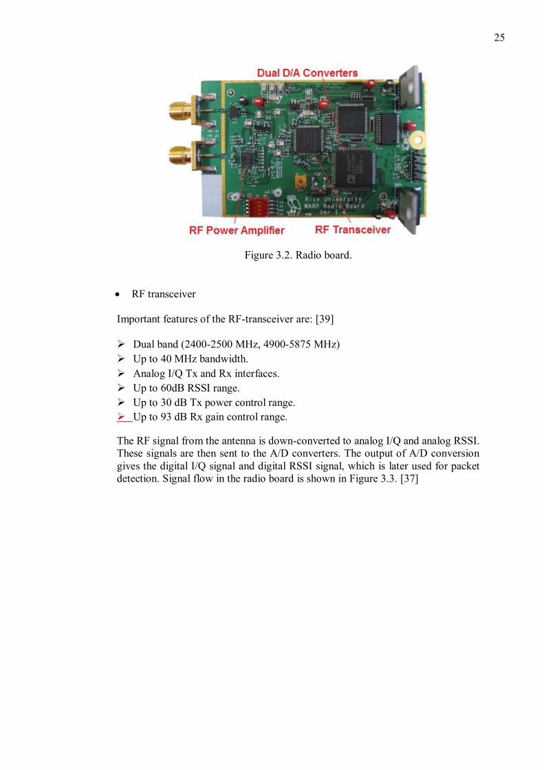
Figure 3.2. Radio board.

RF transceiver

Important features of the RF-transceiver are: [39]

Dual band (2400-2500 MHz, 4900-5875 MHz)

Up to 40 MHz bandwidth.

Analog I/Q Tx and Rx interfaces.

Up to 60dB RSSI range.

Up to 30 dB Tx power control range.

Up to 93 dB Rx gain control range.

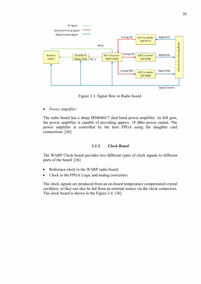
The RF signal from the antenna is down-converted to analog I/Q and analog RSSI.

These signals are then sent to the A/D converters. The output of A/D conversion

gives the digital I/Q signal and digital RSSI signal, which is later used for packet

detection. Signal flow in the radio board is shown in Figure 3.3. [37]

26

Figure 3.3. Signal flow in Radio board.

Power Amplifier

The radio board has a sharp IRM046U7 dual band power amplifier. At full gain,

the power amplifier is capable of providing approx. 18 dBm power output. The

power amplifier is controlled by the host FPGA using the daughter card

connections. [36]

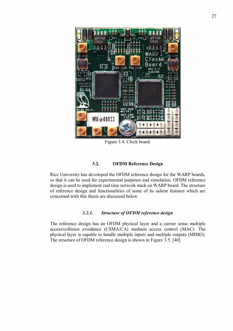
3.1.3. Clock Board

The WARP Clock board provides two different types of clock signals to different

parts of the board: [36]

Reference clock to the WARP radio board.

Clock to the FPGA Logic and analog converters.

The clock signals are produced from an on-board temperature compensated crystal

oscillator, or they can also be fed from an external source via the clock connectors.

The clock board is shown in the Figure 3.4. [36]

27

Figure 3.4. Clock board.

3.2. OFDM Reference Design

Rice University has developed the OFDM reference design for the WARP boards,

so that it can be used for experimental purposes and simulation. OFDM reference

design is used to implement real time network stack on WARP board. The structure

of reference design and functionalities of some of its salient features which are

concerned with this thesis are discussed below.

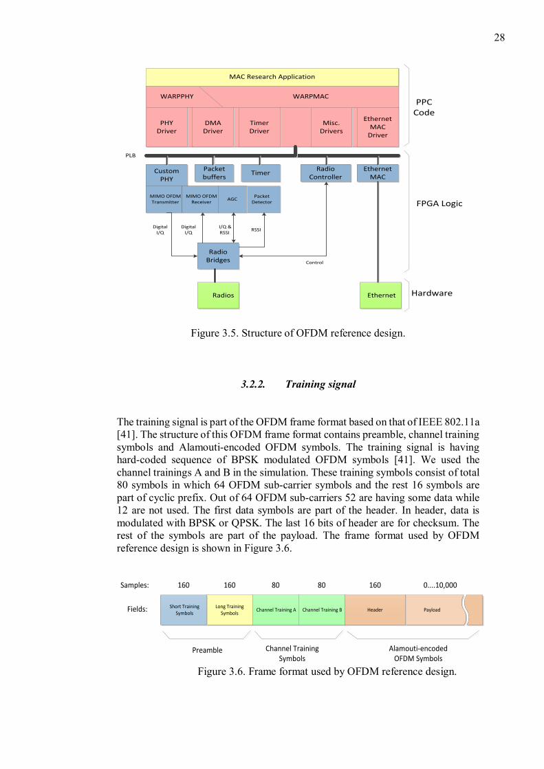
3.2.1. Structure of OFDM reference design

The reference design has an OFDM physical layer and a carrier sense multiple

access/collision avoidance (CSMA/CA) medium access control (MAC). The

physical layer is capable to handle multiple inputs and multiple outputs (MIMO).

The structure of OFDM reference design is shown in Figure 3.5. [40]

28

WARPPHY WARPMAC

PHYDriver

DMADriver

TimerDriver

Misc.Drivers

EthernetMAC

Driver

Ethernet MAC

Custom PHY

AGC

Packet buffers

TimerRadio

Controller

MIMO OFDM Transmitter

MIMO OFDM Receiver

Packet Detector

Radio Bridges

Radios Ethernet

MAC Research Application

PLB

Digital I/Q

Digital I/Q

I/Q & RSSI

RSSI

Control

PPC Code

FPGA Logic

Hardware

Figure 3.5. Structure of OFDM reference design.

3.2.2. Training signal

The training signal is part of the OFDM frame format based on that of IEEE 802.11a

[41]. The structure of this OFDM frame format contains preamble, channel training

symbols and Alamouti-encoded OFDM symbols. The training signal is having

hard-coded sequence of BPSK modulated OFDM symbols [41]. We used the

channel trainings A and B in the simulation. These training symbols consist of total

80 symbols in which 64 OFDM sub-carrier symbols and the rest 16 symbols are

part of cyclic prefix. Out of 64 OFDM sub-carriers 52 are having some data while

12 are not used. The first data symbols are part of the header. In header, data is

modulated with BPSK or QPSK. The last 16 bits of header are for checksum. The

rest of the symbols are part of the payload. The frame format used by OFDM

reference design is shown in Figure 3.6.

Long Training Symbols

Channel Training A Channel Training B HeaderShort Training

SymbolsPayloadFields:

Samples: 160 160 80 80 160 0....10,000

Preamble Channel Training Symbols

Alamouti-encoded OFDM Symbols

Figure 3.6. Frame format used by OFDM reference design.

29

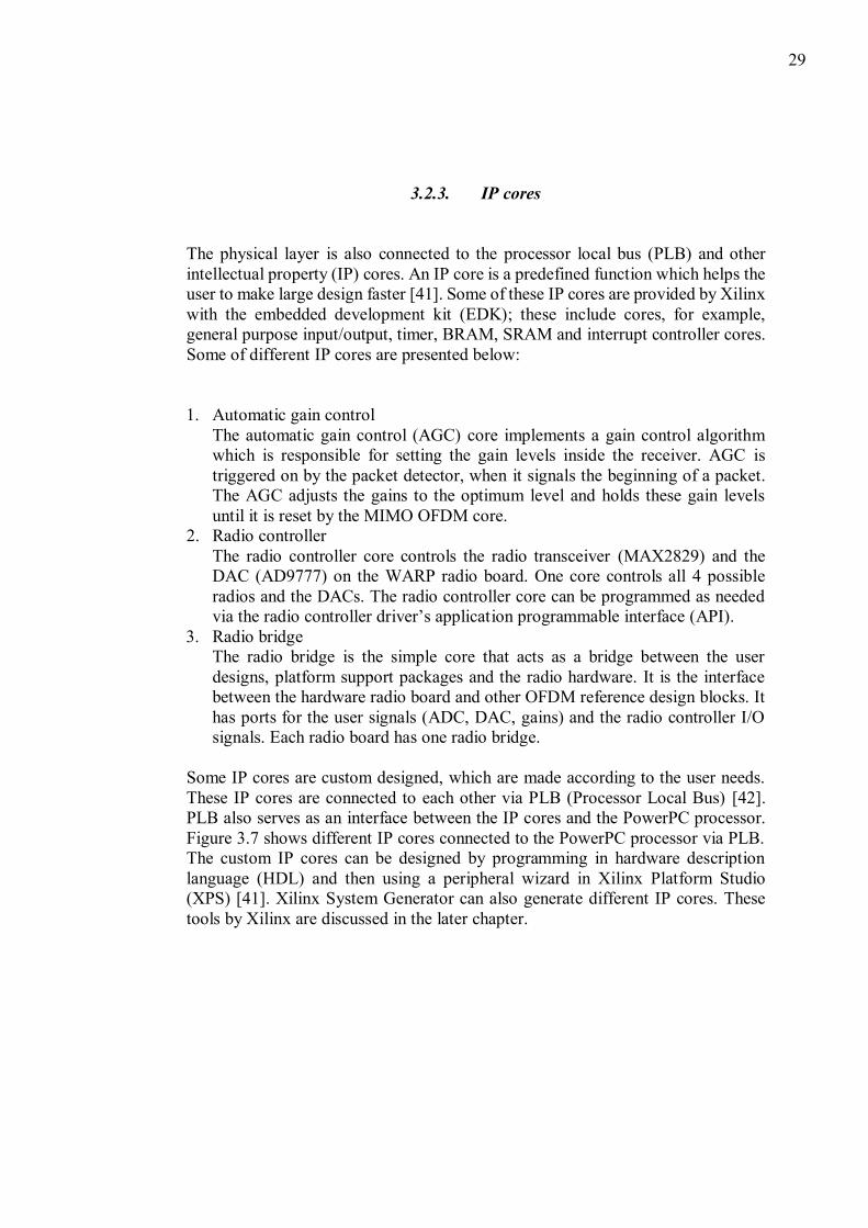
3.2.3. IP cores

The physical layer is also connected to the processor local bus (PLB) and other

intellectual property (IP) cores. An IP core is a predefined function which helps the

user to make large design faster [41]. Some of these IP cores are provided by Xilinx

with the embedded development kit (EDK); these include cores, for example,

general purpose input/output, timer, BRAM, SRAM and interrupt controller cores.

Some of different IP cores are presented below:

1. Automatic gain control

The automatic gain control (AGC) core implements a gain control algorithm

which is responsible for setting the gain levels inside the receiver. AGC is

triggered on by the packet detector, when it signals the beginning of a packet.

The AGC adjusts the gains to the optimum level and holds these gain levels

until it is reset by the MIMO OFDM core.

2. Radio controller

The radio controller core controls the radio transceiver (MAX2829) and the

DAC (AD9777) on the WARP radio board. One core controls all 4 possible

radios and the DACs. The radio controller core can be programmed as needed

via the radio controller driver’s application programmable interface (API).

3. Radio bridge

The radio bridge is the simple core that acts as a bridge between the user

designs, platform support packages and the radio hardware. It is the interface

between the hardware radio board and other OFDM reference design blocks. It

has ports for the user signals (ADC, DAC, gains) and the radio controller I/O

signals. Each radio board has one radio bridge.

Some IP cores are custom designed, which are made according to the user needs.

These IP cores are connected to each other via PLB (Processor Local Bus) [42].

PLB also serves as an interface between the IP cores and the PowerPC processor.

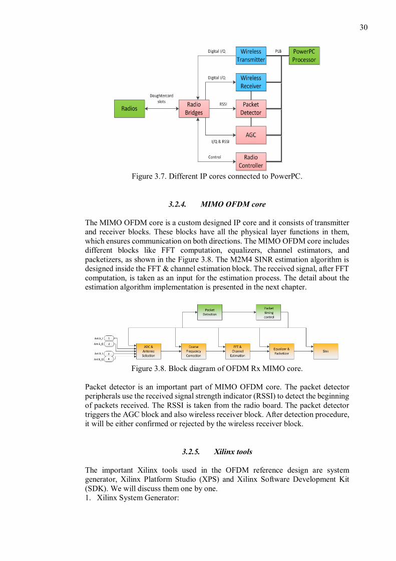
Figure 3.7 shows different IP cores connected to the PowerPC processor via PLB.

The custom IP cores can be designed by programming in hardware description

language (HDL) and then using a peripheral wizard in Xilinx Platform Studio

(XPS) [41]. Xilinx System Generator can also generate different IP cores. These

tools by Xilinx are discussed in the later chapter.

30

Figure 3.7. Different IP cores connected to PowerPC.

3.2.4. MIMO OFDM core

The MIMO OFDM core is a custom designed IP core and it consists of transmitter

and receiver blocks. These blocks have all the physical layer functions in them,

which ensures communication on both directions. The MIMO OFDM core includes

different blocks like FFT computation, equalizers, channel estimators, and

packetizers, as shown in the Figure 3.8. The M2M4 SINR estimation algorithm is

designed inside the FFT & channel estimation block. The received signal, after FFT

computation, is taken as an input for the estimation process. The detail about the

estimation algorithm implementation is presented in the next chapter.

Figure 3.8. Block diagram of OFDM Rx MIMO core.

Packet detector is an important part of MIMO OFDM core. The packet detector

peripherals use the received signal strength indicator (RSSI) to detect the beginning

of packets received. The RSSI is taken from the radio board. The packet detector

triggers the AGC block and also wireless receiver block. After detection procedure,

it will be either confirmed or rejected by the wireless receiver block.

3.2.5. Xilinx tools

The important Xilinx tools used in the OFDM reference design are system

generator, Xilinx Platform Studio (XPS) and Xilinx Software Development Kit

(SDK). We will discuss them one by one.

1. Xilinx System Generator:

31

Xilinx System Generator is one of the key components used in digital signal

processing (DSP) targeted design platforms. It provides system modeling and

automatic code generation from Simulink. One of the key features of systems

generator is to build and debug high-performance DSP systems in Simulink by

using Xilinx blockset; that contains functions for signal processing, error

correction, arithmetic operations, memories and digital logic [43]. It also

supports bit and cycle accurate floating and fixed point implementation. It also

implements automatic code generation of VHDL or Verilog from Simulink; it

targets specific IP cores from Xilinx blockset and also supports custom HDL

through its HDL import flow [43]. It develops highly parallel systems with

advanced FPGAs. System generator provides shared memory abstraction of the

HW/SW interface, automatically generating the bus interface logic and software

drivers.

2. Xilinx Platform Studio:

Xilinx Platform Studio (XPS) is an important component of the Xilinx

integrated software environment (ISE); which is designed for synthesis and

analysis of HDL designs to enable the hardware designers to easily built,

connect and configure embedded processor based systems. The true potential of

XPS is its ability to configure plug and play IP cores from Xilinx embedded IP

library. It also provides flexibility to design highly custom processors according

to the project needs. It employs graphical design views and also provides correct

by design wizard to help designers to design custom processor systems in a short

time [44].

3. Xilinx Software Development Kit:

Xilinx Software Development Kit (SDK) is the complete integrated design

environment (IDE) for creating powerful and optimized software applications

for all Xilinx embedded microprocessors. It provides complete software design

and supports debug flows including multicore and hardware/software debug

capabilities. It supports custom libraries and device drivers [45].

32

4. IMPLEMENTATION OF M2M4 ALGORITHM

The algorithm which was chosen for the implementation of the SINR estimation is

M2M4, also described in chapter 2. The algorithm was simulated in different

scenarios (i.e., for different SINR levels as input) in order to check its behavior and

verify its performance. The algorithm was simulated in MATLAB and then

designed in system generator model. The estimator was designed using the system

generator model of the OFDM reference design and a custom block was added

inside the FFT and channel estimation block in the OFDM Rx MIMO IP core.

Performance verification is done by using the same input SNR for MATLAB

simulations as well as for the system generator model. The process is repeated

several times, for each channel SNR, to check the validity of the results. The

comparison is drawn between simulations and system generator model.

4.1. Design Consideration

As discussed earlier this is non-data aided estimator therefore, it is not required to

determine training signals for SINR estimation. In the current scenario, training

signal is only required for the timing synchronization with the received signal,

without the phase information of the training symbols. The description of the

training signal used is already presented in Chapter 3. Presently, we assume that the

receiver has already done the time synchronization and thus phase estimation is not

required before the SINR estimation, which simplifies the operation of the

estimator. Since the modulation method is known to us, hence we used the training

signal to create the realistic scenario for the SINR estimation. We used the same

training signal, which was used by the OFDM reference design as discussed in

section 3.2.2. The training signal is represented mathematically by a vector having

1,-1 and 0 as its elements, where 1 and -1 show the discreet signal amplitudes and

0 depicts no signal. The training signal contains 64 OFDM sub-carrier symbols, out

of which 52 are used while 12 are not used.

The channel is simulated using Monte Carlo simulation method, which is used to

determine the sensitivity of a complex system by varying system parameters [46].

In this case, the system parameters are random phase; noise and SNR. The training

signal is multiplied with the random complex exponential to simulate the random

phase. Secondly, additive white Gaussian noise (AWGN) is introduced for each

SNR level to simulate the received signal, having noise and interference in it. The

channel SNR is increased sequentially with a constant step of 5 dB.

The received signal is squared for each sample and the mean is computed. This

yields second order moment (𝑀2), as shown in equation (41) and (42). The squared

samples are again squared and the mean computation gives fourth order moment

(𝑀4), as shown in equation (43). The 𝑀4 is subtracted from two times squared 𝑀2,

square root of the resultant gives the received signal power (𝑃𝑑), as shown in

equation (44). The 𝑃𝑑 is subtracted from 𝑀2, which yields Interference plus Noise

power (𝑃𝑛), as shown in equation (45). SINR can be computed by the ratio of 𝑃𝑑 and 𝑃𝑛, as shown in equation (46). All of the above mentioned mathematical

calculations are done by using a nested loop. Then the mean of estimated SINR is

33

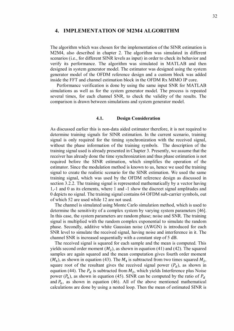
calculated for each channel SNR level. All the mathematical calculations are shown

in the form of block diagram in Figure 4.1.

Figure 4.1. Block diagram of M2M4 estimator.

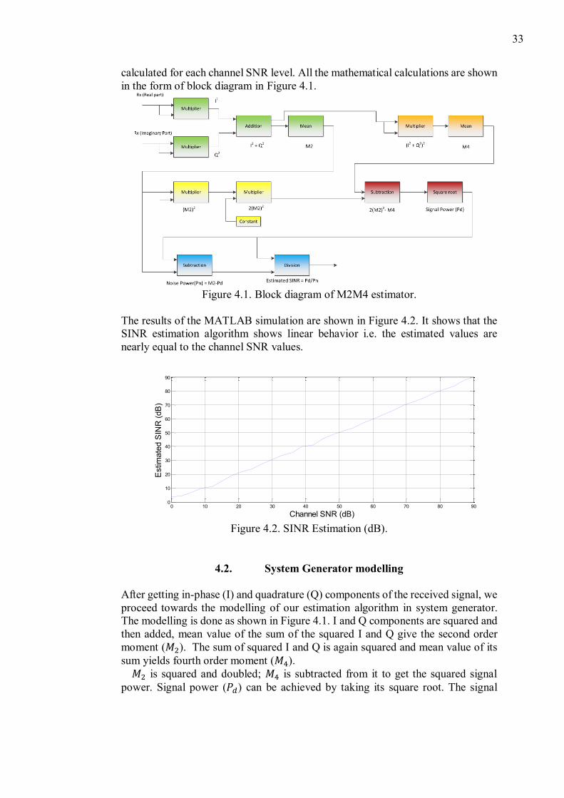
The results of the MATLAB simulation are shown in Figure 4.2. It shows that the

SINR estimation algorithm shows linear behavior i.e. the estimated values are

nearly equal to the channel SNR values.

Figure 4.2. SINR Estimation (dB).

4.2. System Generator modelling

After getting in-phase (I) and quadrature (Q) components of the received signal, we

proceed towards the modelling of our estimation algorithm in system generator.

The modelling is done as shown in Figure 4.1. I and Q components are squared and

then added, mean value of the sum of the squared I and Q give the second order

moment (𝑀2). The sum of squared I and Q is again squared and mean value of its

sum yields fourth order moment (𝑀4).

𝑀2 is squared and doubled; 𝑀4 is subtracted from it to get the squared signal

power. Signal power (𝑃𝑑) can be achieved by taking its square root. The signal

0 10 20 30 40 50 60 70 80 900

10

20

30

40

50

60

70

80

90

Channel SNR (dB)

Estim

ate

d S

INR

(dB

)

34

power is subtracted from 𝑀2 to get the noise power (𝑃𝑛). The SINR estimate can be

calculated from the ratio of 𝑃𝑑 and 𝑃𝑛.

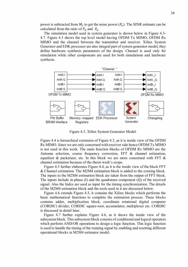
The simulation model used in system generator is shown below in Figure 4.3-

4.7. Figure 4.3 shows the top level model having OFDM Tx MIMO, OFDM Rx

MIMO and the channel between the transmitter and receiver. Xilinx System

Generator and EDK processor are also integral part of system generator model, they

define hardware synthesis parameters of the design. Channel is used only for

simulation while other components are used for both simulations and hardware

synthesis.

Figure 4.3. Xilinx System Generator Model.

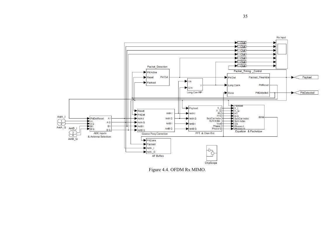
Figure 4.4 is hierarchical extension of Figure 4.3, as it is inside view of the OFDM

Rx MIMO. Since we are only concerned with receiver side hence OFDM Tx MIMO

is not used in this work. The main function blocks of OFDM Rx MIMO are the

Antenna selection, coarse frequency correction, FFT & channel estimation,

equalizer & packetizer, etc. In this block we are more concerned with FFT &

channel estimation because of the thesis work’s scope.

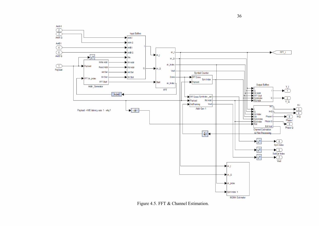
Figure 4.5 further elaborates Figure 4.4, as it is the inside view of the block FFT

& Channel estimation. The M2M4 estimation block is added to the existing block.

The inputs to the M2M4 estimation block are taken from the output of FFT block.

The inputs include in-phase (I) and the quadrature component (Q) of the received

signal. Also the Index are used as input for the timing synchronization. The details

of the M2M4 estimation block and the tools used in it are discussed below.

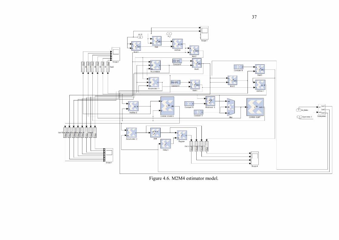
Figure 4.6 extends Figure 4.5, it contains the Xilinx blocks which performs the

basic mathematical functions to complete the estimation process. These blocks

contains adder, multiplication block, coordinate rotational digital computer

(CORDIC) divider, CORDIC square-root, accumulator, multiplexer etc. CORDIC

is discussed in detail later.

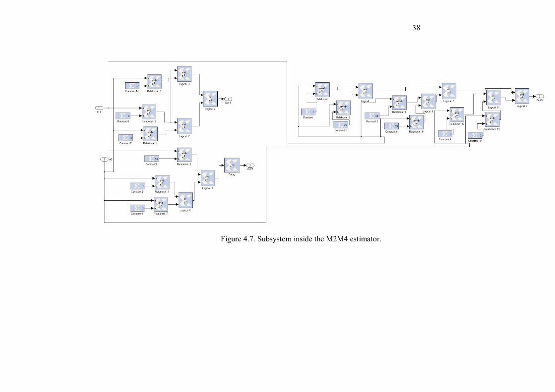
Figure 4.7 further explains Figure 4.6, as it shows the inside view of the

subsystem block. This subsystem block consists of conditional and logical operators

which perform AND/OR operations to design a logic function. This logic function

is used to handle the timing of the training signal by enabling and resetting different

operational blocks in M2M4 estimator model.

35

Figure 4.4. OFDM Rx MIMO.

36

Figure 4.5. FFT & Channel Estimation.

37

Figure 4.6. M2M4 estimator model.

38

Figure 4.7. Subsystem inside the M2M4 estimator.

39

4.2.1. Word-length and binary point

Word-length is an important parameter to discuss in regard to the implementation

of M2M4 SINR estimator. Word-length is the data handling capacity, i.e., input or

output of a processor block (in bits). For example, if word length is equal to 5 bits

and all bits are dedicated for integer part then it means that the maximum value that

can be stored in that is 25-1, i.e., 31 in decimal number format. In the simulations

we used fixed point numbers, which contain an integer followed by its fractional

part. Since in DSP systems, a real number is represented in binary number format

therefore we use binary point in fixed point numbers. Binary point is analogous to

the decimal point in the decimal number format. If some calculations results in

negative number, we dedicate a separate bit, called sign bit.

The number of bits show the total number of bits or word-length which one block

can process or compute; binary point is the fractional part of that number. Table 1

shows the word-lengths and binary point used by each component of the M2M4

estimator design. In the following table “Addsub” block had 16 bits word-length

and the binary point is also 16 it means that the input to this block just is a small

fraction so that we use all the bits to represent the fractional part. Likewise, for the

block “constant-8”, word-length is 16 but the fractional part is 15, input to or from

this block is a number which can be represented in 1 bit but the rest 15 bits are

allocated for the binary point.

Table 1. Word-lengths of M2M4 estimator components

Component

name

Number

of bits

Binary

Point

Accumulator 16 -

Accumulator-1 16 -

Accumulator-2 30 -

Addsub 16 16

Addsub-1 18 18

Addsub-2 16 16

Constant-8 16 15

Constant-9 16 15

Constant-10 16 14

Constant-11 16 16

Constant-12 16 16

Cordic divider 24 20

Cordic sqrt 18 18

Mult 16 16

Mult-1 16 16

Mult-2 16 16

Mult-3 18 16

Mult-4 16 16

Mult-5 18 16

Mult-6 18 18

40

Mux 18 18

Shift 16 14

4.2.2. Introduction to CORDIC

Complex arithmetic operations are the fundamentals of any DSP system.

Numerous DSP algorithms rely heavily on different trigonometric, arithmetic and

complex computations. In order to estimate these computations, different

algorithms have been proposed in recent years. One of the widely practiced and

intuitively simple algorithm is Coordinate Rotation Digital Computer algorithm

(CORDIC). In a nutshell, the methodology computes by iterative sequence of

addition, subtraction and shift operations. CORDIC iterations can be computed

using the following equations:

𝑥𝑖+1 = 𝑥𝑖 − 𝑚. 𝜇𝑖 . 𝑦𝑖 . 𝛿𝑚,𝑖 (47)

𝑦𝑖+1 = 𝑦𝑖 + 𝜇𝑖 . 𝑥𝑖. 𝛿𝑚,𝑖 (48)

𝑧𝑖+1 = 𝑧𝑖 − 𝜇𝑖 . 𝛼𝑚,𝑖 (49)

The variable 𝑚 specifies the coordinate system i.e. circular, linear or hyperbolic.

The rotation angle 𝛼𝑚,𝑖 is observed by the variable 𝑧𝑖 . The variable 𝜇𝑖 defines the

rotation direction. In order to avoid multiplications, the variable 𝛿𝑚,𝑖 is defined as:

𝛿𝑚,𝑖 = 𝑑−𝑠𝑚,𝑖 (50)

𝛿𝑚,𝑖 = 2−𝑠𝑚,𝑖 (51)

Less hardware cost makes CORDIC a utility in the practical world. Besides being

cost effective CORDIC is relatively simple. It uses bit shift operations such as (2

adders + 2 shifters) instead of (4 multiplier + 2 adders). However, as also discussed

by [47], CORDIC has some design considerations, it takes N iterations to achieve

n-bit precision. Secondly, the carry propagate mechanism is slow. Additionally, it

has a low throughput rate and occupies a large area for the computation of shift

operations. Also Zhang et al mentioned in [48], because of less coverage angle and

increased pipeline series, CORDIC consumes lot of hardware resources and has

limited processing speed.

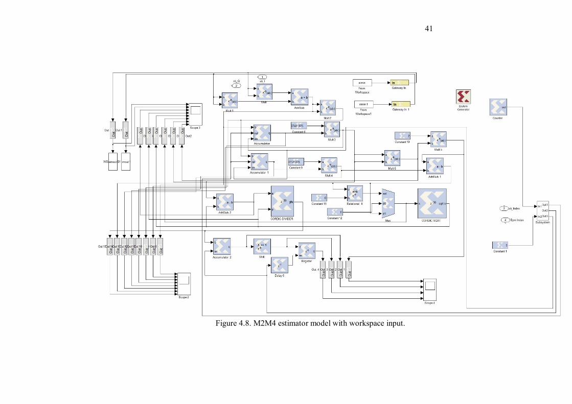
4.3. Performance Verification

The MATLAB simulation, which is discussed in section 4.1, returns SINR value

for a given channel SNR. The performance of estimator was verified by using the

same channel SNR as input to the system generator model, and then compared with

the simulation. The channel SNR range used for performance verification is from 5

dB to 40 dB. The function block “simin” is used to input the data from the

simulation workspace to the reference design. Figure 4.8 shows the model designed

to test and verify the performance of M2M4 estimator.

41

Figure 4.8. M2M4 estimator model with workspace input.

42

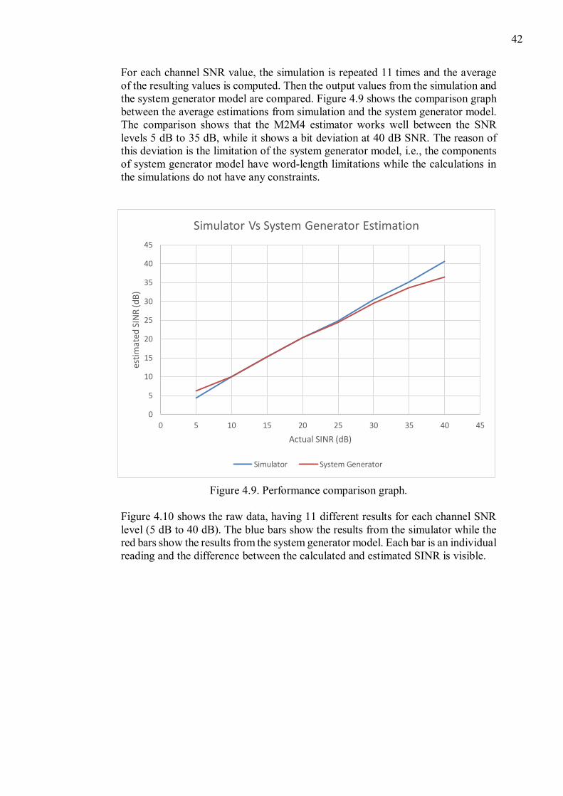
For each channel SNR value, the simulation is repeated 11 times and the average

of the resulting values is computed. Then the output values from the simulation and

the system generator model are compared. Figure 4.9 shows the comparison graph

between the average estimations from simulation and the system generator model.

The comparison shows that the M2M4 estimator works well between the SNR

levels 5 dB to 35 dB, while it shows a bit deviation at 40 dB SNR. The reason of

this deviation is the limitation of the system generator model, i.e., the components

of system generator model have word-length limitations while the calculations in

the simulations do not have any constraints.

Figure 4.9. Performance comparison graph.

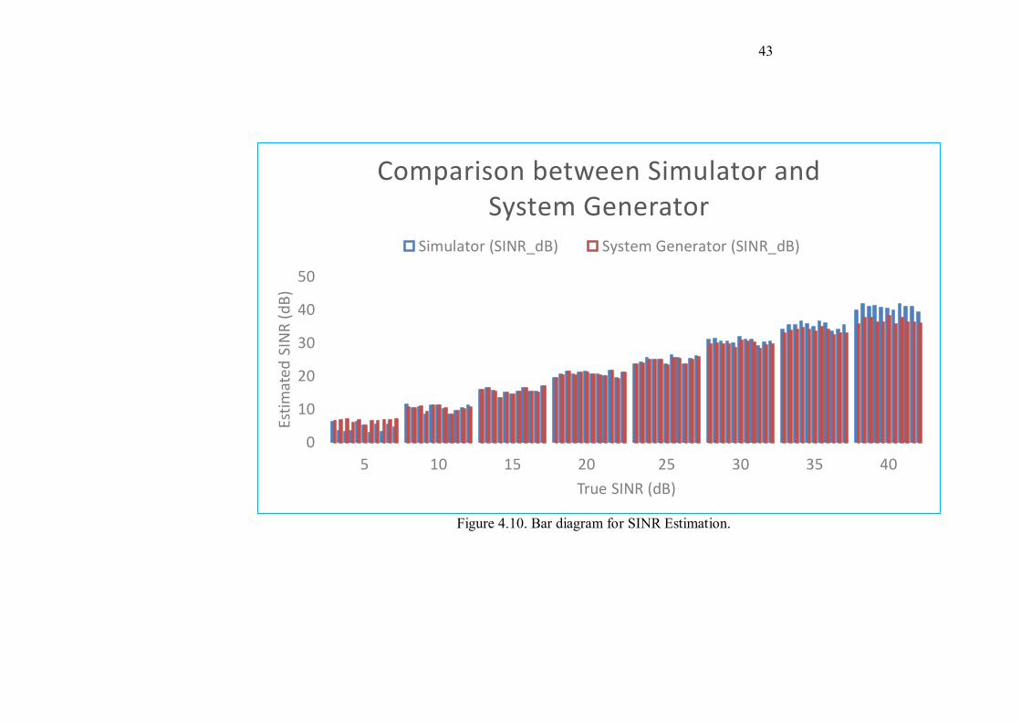
Figure 4.10 shows the raw data, having 11 different results for each channel SNR

level (5 dB to 40 dB). The blue bars show the results from the simulator while the

red bars show the results from the system generator model. Each bar is an individual

reading and the difference between the calculated and estimated SINR is visible.

0

5

10

15

20

25

30

35

40

45

0 5 10 15 20 25 30 35 40 45

esti

mat

ed S

INR

(dB

)

Actual SINR (dB)

Simulator Vs System Generator Estimation

Simulator System Generator

43

Figure 4.10. Bar diagram for SINR Estimation.

0

10

20

30

40

50

5 10 15 20 25 30 35 40

Esti

mat

ed

SIN

R (

dB

)

True SINR (dB)

Comparison between Simulator and System Generator

Simulator (SINR_dB) System Generator (SINR_dB)

44

5. DISCUSSION

In this section, three general subtopics related to the thesis work are discussed: (a)

problems, (b) alternate methods, and (c) future improvements.

The main problem faced in the thesis was that the design could not be fitted into

the WARP hardware. One reason of this was the heavy design which consumes

more resources than available in the hardware. CORDIC square-root and CORDIC

divider blocks are used in the design, which occupies a lot of hardware resources

and they require large word-length for precise calculations. In the recent years,

pipelined architecture became the most suitable architecture for CORDIC.

However, as discussed in previous chapter, the computational cost cannot be

undermined. Recently, researchers have proposed CORDIC using less number of

iterations and optimized shift sequences for acceptable level of accuracy.

The word-length adjustment is an important issue because of quantization effect,

since we are using the quantized data for mathematical calculations in real time

DSP systems. The word-lengths of different components in the system generator

model are presented in Table 1. It is clear from the Table 1 that CORDIC square-

root and CORDIC divider are inefficient in terms of hardware consumption, as

compared to others, and since they are having more word-lengths; the calculation

is complex. In other words, the SINR estimation model we designed require more

FPGA hardware resources than available.

Figure 4.8 shows the comparison between the simulation and system generator

model. It shows that the M2M4 estimator works efficiently in the range from 5 dB

to 35 dB SINR level. It deviates from the curve at 40 dB SINR level which is

because of word-length limitation of the system generator model, i.e. , the precision

of model is limited due to the restricted word-length. This constraint cannot be

observed in simulations, hence the results are different at higher SINR levels.

Alternative methods can be adopted to fit this design into the WARP FPGA chip.

We suggested the use of functional blocks other than CORDIC square-root and

CORDIC divider blocks, which uses less hardware resources. Smartly selecting

application specific blocks rather than CORDIC blocks, will also reduce the

complexity of the design. Experimental evaluation also revealed that by using look-

up table for computing the square-root and division results in low resource

occupation.

Further improvements can also be done in the existing design in the future. In

[49] Bertrand mentions that generating of hardware architecture is complex

because word-lengths should be analyzed in depth to determine exactly what kind

of hardware resources are needed. He also proposed an automated design

methodology which is based on high-level synthesis.

45

6. SUMMARY

The aim of the thesis is to introduce an efficient SINR estimation algorithm for

WARP. The thesis is a part of CORE project which aims to develop a testing

environment to test cognitive functionalities on different wireless environments.

SINR estimation algorithm named M2M4 is proposed for implementation on

WARP.

The SINR plays an important role in wireless networks because many

functionalities need to know the link quality. Depending upon the amount of

information available in the received signal, SINR estimators are categorized into

two types: data aided (DA) and non-data aided (NDA). During the past few decades,

a lot of different SINR estimation techniques have been developed. Different SINR

estimation techniques have been studied, for example SSME, ML, SNV and M2M4.

After studying different SINR estimation techniques, M2M4 estimation algorithm

is chosen for the thesis work because it has low computational complexity. Also it

has a linear response and no upper limit for estimation.

Implementation was done on wireless open-access research platform (WARP)

and the important functionalities of WARP were discussed in this work. WARP has

been developed by center for multimedia communications at Rice University, USA.

WARP consists of FPGA chip hardware and a reference design. The FPGA chip in

WARP is Xilinx Virtex-4 FPGA chip. Combination of hardware and reference

design makes a complete OFDM communication system. WARP is a flexible test

platform and it is programmable. Hence it can be used for implementation of

customized physical layer and MAC layer. M2M4 estimation algorithm was

implemented with reference design to enable the use of SINR estimation

information for future research.

M2M4 estimation algorithm is first simulated in MATLAB and then it is

designed for WARP using Xilinx System Generator tool. System generator is

digital logic design tool which works with MATLAB Simulink and it is capable of

generating HDL codes for hardware implementation. M2M4 estimation algorithm

is simulated in different environments by taking different SINR levels as input, to

check its behavior. Also the performance of the estimator is verified by using the

input from the MATLAB program to the system generator. The same simulation is

repeated 11 times to get better average values and the results are compared. The

comparison shows that M2M4 estimator is efficient.

The results proved that the estimator is working efficiently. The M2M4 estimator

design could not be fitted into the WARP because the hardware requirements for

this design are very high. In other words, the design require more FPGA resources.

CORDIC square root and CORDIC divider are the most resource consuming

components. Eyeing the future work in hardware systems, we suggest

improvements in CORDIC square root and CORDIC divider components, as their

resource consumption makes them inefficient for many practical applications. We

suggest and demonstrated that one of the alternatives for CORDIC components

could be look up tables. For the future work, we plan to implement the same design

using other components which do not require much hardware resources.

46

7. REFERENCES

[1] Zivkovic, M.; Mathar, R., "An improved preamble-based SNR estimation

algorithm for OFDM systems," Personal Indoor and Mobile Radio

Communications (PIMRC), 2010 IEEE 21st International Symposium on

, vol., no., pp.172,176, 26-30 Sept. 2010

URL: http://ieeexplore.ieee.org/stamp/stamp.jsp?tp=&arnumber=56719

16&isnumber=5671569

[2] LTE standard specifications (accessed on July 25 2012) URL:

http://www.3gpp.org/lte

[3] Hoikkanen A. (2007) Economics of 3G Long-Term Evolution: the

Business Case for the Mobile Operator. In: IFIP International Conference

on Wireless and Optical Communications Networks, July 2-4, p.1-5.

[4] Zhao X., Guo Z. & Guo Q. (2010) A Cognitive Based Spectrum Sharing

Scheme for LTE Advanced Systems.

In:International Congress on Ultra Modern Telecommunications and

Control Systems and Workshops (ICUMT), October 18-20, p. 965-969.

[5] Lien S. & Chen K. (2011) Statistical Traffic Control For Cognitive Radio

Empowered LTE-Advanced with Network MIMO. In: IEEE Conference

on Computer Communications Workshops (INFOCOM), April 10-15,

p.80-84.

[6] Federal Communications Commission (2002) Spectrum Policy Task

force Report, ET Docket No. 02-135.

[7] Pan M., Zhang C., Li P. & Fang Y. (2011) Joint Routing and Link

Scheduling for Cognitive Radio Networks under Uncertain Spectrum

Supply. In: IEEE Proceedings of INFOCOM, April 10-15, p.2237-2245.

[8] Matinmikko M. (2012) Spectrum sharing using cognitive radio system

capabilities: Methods to obtain and exploit knowledge of spectrum

availability, Ph.D. dissertation, VTT Technical Research Centre, Finland.

[9] Mitola J. (2000) Cognitive radio: integrated agent architecture for

software defined radio, Ph.D. dissertation, Royal Institute of Technology

(KTH), Sweden.

[10] Lopez-Valcarce, R.; Mosquera, C., "Sixth-Order Statistics-Based Non-

Data-Aided SNR Estimation," Communications Letters, IEEE , vol.11,

no.4, pp.351,353, April 2007


40&isnumber=4155617

http://ieeexplore.ieee.org/stamp/stamp.jsp?tp=&arnumber=5671916&isnumber=5671569






47

[11] Ong, Sylvia Ai Ling (2012) SNR estimation using extended kalman filter

technique for orthogonal frequency division multiplexing (OFDM)

system. Masters thesis, Universiti Tun Hussein Onn Malaysia.

[12] Xiaodong Xu; Ya Jing; Xiaohu Yu, "Subspace-based noise variance and

SNR estimation for OFDM systems [mobile radio applications],"

Wireless Communications and Networking Conference, 2005 IEEE ,

vol.1, no., pp.23,26 Vol. 1, 13-17 March 2005.


70&isnumber=30728

[13] Matzner R. An SNR estimation algorithm for complex baseband signals

using higher order statistics. Facta Universitatis (Ni\\u s), 6(1):41–52,

1993.

[14] CORE project (2012), CWC University of Oulu. URL:

http://www.cwc.oulu.fi/researchseminar2012/project_core.html.

[15] Matzner, R.; Englberger, F.; "An SNR estimation algorithm using fourth-

order moments," Information Theory, 1994. Proceedings., 1994 IEEE

International Symposium on , vol., no., pp.119, 27 Jun-1 Jul 1994.

URL:http://ieeexplore.ieee.org/stamp/stamp.jsp?tp=&arnumber=394869

&isnumber=8959

[16] Dahlman, E., Parkvall, S., Skold, J., & Beming, P. (2010). 3G evolution:

HSPA and LTE for mobile broadband. Academic press.

[17] M. Batariere, K. Baum and T. P. Krauss, "Cyclic prefix length analysis

for 4G OFDM systems," Vehicular Technology Conference, 2004.

VTC2004-Fall. 2004 IEEE 60th, 2004, pp. 543-547 Vol. 1.

doi: 10.1109/VETECF.2004.1400066.


66&isnumber=30410

[18] Shahabuddin, S., & Juntti, M. DESIGN OF APPLICATION-SPECIFIC

SIGNAL PROCESSORS FOR ITERATIVE TURBO DECODER.

[19] Das, A., & Rao, B. D. (2012). SNR and noise variance estimation for

MIMO systems. Signal Processing, IEEE Transactions on, 60(8), 3929-

3941.

[20] Balachandran, K.; Kadaba, S.R.; Nanda, S., "Channel quality estimation

and rate adaptation for cellular mobile radio," Selected Areas in

Communications, IEEE Journal on , vol.17, no.7, pp.1244,1256, Jul 1999


3&isnumber=16902



http://www.cwc.oulu.fi/researchseminar2012/project_core.html







48

[21] Zander, J., "Performance of optimum transmitter power control in

cellular radio systems," Vehicular Technology, IEEE Transactions on ,

vol.41, no.1, pp.57,62, Feb 1992


5&isnumber=3431

[22] Summers T. A. and Wilson S. G. , "SNR Mismatch and Online

Estimation in Turbo Decoding", IEEE Trans. Commun., vol. 46, no. 4,

pp 421-423, Apr. 1998.

[23] Linn, Y., "A Carrier-Independent Non-Data-Aided Real-Time SNR

Estimator for M-PSK and D-MPSK Suitable for FPGAs and ASICs,"

Circuits and Systems I: Regular Papers, IEEE Transactions on , vol.56,

no.7, pp.1525,1538, July 2009


72&isnumber=5153552

[24] Yunfei Chen; Beaulieu, N.C., "NDA estimation of SINR for QAM

signals," Communications Letters, IEEE , vol.9, no.8, pp.688,690, Aug

2005


83&isnumber=32148

[25] Sorooshyari, S.; Chee-wei Tan; Poor, H.V., "On Maximum-Likelihood

SINR Estimation of MPSK in a Multiuser Fading Channel," Vehicular

Technology, IEEE Transactions on , vol.59, no.8, pp.4175,4181, Oct.

2010.


62&isnumber=5601981

[26] Haifeng Xiao; Shi, Y.Q.; Wei Su; Kosinski, J., "An investigation of non-

data-aided SNR estimation techniques for analog modulation signals,"

Sarnoff Symposium, 2010 IEEE , vol., no., pp.1,5, 12-14 April 2010.


06&isnumber=5469698

[27] Pauluzzi, D.R.; Beaulieu, N.C., "A comparison of SNR estimation

techniques for the AWGN channel," Communications, IEEE

Transactions on , vol.48, no.10, pp.1681,1691, Oct 2000.


3&isnumber=18877

[28] Shah, B.; Hinedi, S., "The split symbol moments SNR estimator in

narrow-band channels," Aerospace and Electronic Systems, IEEE

Transactions on, vol.26, no.5, pp.737,747, Sep 1990.


9&isnumber=3173

[29] Gagliardi, R.M.; Thomas, C., "PCM Data Reliability Monitoring

Through Estimation of Signal-to-Noise Ratio," Communication















49

Technology, IEEE Transactions on , vol.16, no.3, pp.479,486, June 1968.


51&isnumber=23719

[30] Gilchriest C.E. , "Signal-to-noise monitoring," JPL Space Programs

Summary, vol. IV, no. 37-27, pp. 169-184, June 1966.

[31] A. L. Brandão, L. B. Lopes, and D. C. McLernon, “In-service monitoring

of multipath delay and cochannel interference for indoor mobile

communication systems,” Proc. IEEE Int. Conf. Communications, vol. 3,

pp. 1458–1462, May 1994.

[32] C. M. Thomas, “Maximum Likelihood Estimation of Signal-to-Noise

Ratio,” Ph.D. dissertation, Univ. of Southern California, Los Angeles,

1967.

[33] Sui Dan; Ge Lindong, "On the Blind SNR Estimation for IF Signals,"

Innovative Computing, Information and Control, 2006. ICICIC '06. First

International Conference on , vol.2, no., pp.374,378, Aug. 30 2006-Sept.

1 2006.


04&isnumber=35657

[34] Sui Dan; Ge Lindong, "A Blind SNR Estimator for Digital Bandpass

Signals," ITS Telecommunications Proceedings, 2006 6th International

Conference on , vol., no., pp.1334,1337, June 2006.


35&isnumber=4068498

[35] Matzner R., Engleberger F., and Siewert R., “Analysis and design of a

blind statistical SNR estimator,” in AES 102nd Convention, München,

Germany, Mar. 1997.

[36] Hardware User Guide, FPGA Board V2.2, Rice University, USA.

http://warpproject.org/trac/wiki/HardwareUsersGuides/FPGABoard_v2.

2 (accessed on 3 March 2014)

[37] Hanninen, T.; Vartiainen, J.; Juntti, M.; Raustia, M.; , "Implementation

of spectrum sensing on wireless open-access research platform," Applied

Sciences in Biomedical and Communication Technologies (ISABEL),

2010 3rd International Symposium on , vol., no., pp.1-5, 7-10 Nov. 2010


10&isnumber=5702759

[38] http://warpproject.org/trac/wiki/HardwareUsersGuides/RadioBoard_v1.

4 (accessed on 18 July 2013)

[39] http://warpproject.org/trac/wiki/HardwareUsersGuides/RadioBoard_v1.

4/RF (accessed on 18 July 2013)







http://warpproject.org/trac/wiki/HardwareUsersGuides/FPGABoard_v2.2

http://warpproject.org/trac/wiki/HardwareUsersGuides/FPGABoard_v2.2



http://warpproject.org/trac/wiki/HardwareUsersGuides/RadioBoard_v1.4

http://warpproject.org/trac/wiki/HardwareUsersGuides/RadioBoard_v1.4

http://warpproject.org/trac/wiki/HardwareUsersGuides/RadioBoard_v1.4/RF

http://warpproject.org/trac/wiki/HardwareUsersGuides/RadioBoard_v1.4/RF

50

[40] http://warpproject.org/trac/wiki/OFDMReferenceDesign (accessed on 24

August 2013)

[41] Murphy, Patrick O. "Design, Implementation and Characterization of a

Cooperative Communications System." Doctoral Thesis, Rice University

URL: http://warpproject.org/w/MurphyPhDThesis

[42] http://warpproject.org/trac/wiki/Exercises/13_4/IntroToXPS/w2

(accessed on 24 August 2013)

[43] http://www.xilinx.com/tools/sysgen.htm (Accessed on 2nd April, 2013)

[44] http://www.xilinx.com/tools/xps.htm (Accessed on 2nd April, 2013)

[45] http://www.xilinx.com/tools/sdk.htm (Accessed on 2nd April, 2013)

[46] http://www.mathworks.se/discovery/monte-carlo-simulation.html

(Accessed on 12th May, 2014)

[47] Hu, Y.H., "CORDIC-based VLSI architectures for digital signal

processing," in Signal Processing Magazine, IEEE , vol.9, no.3, pp.16-

35, July 1992.


7&isnumber=3852

[48] Chaozhu Zhang, Jinan Han, and Ke Li, “Design and Implementation of

Hybrid CORDIC Algorithm Based on Phase Rotation Estimation for

NCO,” The Scientific World Journal, vol. 2014, Article ID 897381, 8

pages, 2014.

[49] Bertrand Le Gal, Emmanuel Casseau (2011) Word-Length Aware DSP

Hardware Design Flow Based on High-Level Synthesis, Journal of signal

processing systems.

http://warpproject.org/trac/wiki/OFDMReferenceDesign

http://warpproject.org/w/MurphyPhDThesis

http://warpproject.org/trac/wiki/Exercises/13_4/IntroToXPS/w2

http://www.xilinx.com/tools/sysgen.htm

http://www.xilinx.com/tools/xps.htm

http://www.xilinx.com/tools/sdk.htm

http://www.mathworks.se/discovery/monte-carlo-simulation.html



Date post:	19-Mar-2018
Category:	Documents
Upload:	nguyentram
View:	236 times
Download:	0 times

IMPLEMENTATION CONSIDERATION OF M2M4 SINR ESTIMATION...

Documents