Implementation of Hydro Power Plant

Optimization for Operation and Production

Planning

Oskar Tengberg

Mechanical Engineering, master's level

2019

Luleå University of Technology

Department of Engineering Sciences and Mathematics

Acknowledgement

This thesis could not have been done without the help of the people of Vattenfallwhere I would like to give a special thank to my supervisor Jonas Funkquist forguiding me through the project.

Advice given by Stefan Sandgren and Magnus Lovgren from Vattenfall has beena great help in providing me knowledge and support in the subject. I wouldalso like to thank my colleague Jonas Almgrund from KTH who also worked onthe same project.

Finally I would like to thank Professor Inge Soderkvist at LTU for being myexaminer for this thesis.

i

Abstract

Output power of hydro power plant was modelled and an optimization algorithmwas implemented in a tool for optimizing hydro power plants. The tool max-imizes power output of a hydro power plant by distributing water over a set ofactive units in the power plant which will be used in planning of electricity pro-duction. This tool was built in a MATLAB environment, using the optimizationtoolbox, and a GUI was developed for Vattenfall. The optimization tool wasbased on the same architecture as the current tool used for this kind of optim-ization which is to be replaced by the work presented in this thesis. Therefore,the goal was to achieve the same optimal results as the current optimization tool.

Power output of three of Vattenfall’s hydro power plants were computed andtwo of these plants were optimized. These power output results were comparedto results from the optimization tool currently used. This showed differenceswithin the inaccuracy of measurements of ≤ 0.3%. These three power plantsproved that the new tool is sufficient to replace the current tool but furthertesting is recommended to be conducted on more of Vattenfall’s hydro powerplants to prove its consistency.

ii

Nomenclature

η Efficiency [-]

ρ Density [kg/m3]

a Transformer polynomial constant [-]

b Generator polynomial constant [-]

c Polynomial constant [-]

g Gravitational acceleration [m/s2]

Gi Unit number i [-]

H Hydraulic head [m]

Hbr Gross height [m]

Hf Head loss [m]

Hlwl Lower water level [m]

Huwl Upper water level [m]

m No. of inactive units [-]

n No. of active units [-]

nf No. of water passages [-]

P Power [MW ]

Q Volumetric flow rate [m3/s]

S Active unit combination [-]

iii

Contents

1 Introduction 21.1 Research aim and limitations . . . . . . . . . . . . . . . . . . . . 31.2 General hydro power plants . . . . . . . . . . . . . . . . . . . . . 41.3 Planning of electricity production . . . . . . . . . . . . . . . . . . 71.4 Plant and river optimization . . . . . . . . . . . . . . . . . . . . . 7

2 Literature Review 92.1 Previous Studies on Hydro Unit Optimization . . . . . . . . . . . 92.2 Optimization Algorithms . . . . . . . . . . . . . . . . . . . . . . 92.3 Combinatorial optimization . . . . . . . . . . . . . . . . . . . . . 92.4 Summary & Conclusion of Literature Review . . . . . . . . . . . 10

3 Theory 113.1 General optimization . . . . . . . . . . . . . . . . . . . . . . . . . 113.2 Objective function in hydro power plant optimization . . . . . . 123.3 Problem setup . . . . . . . . . . . . . . . . . . . . . . . . . . . . 163.4 Optimization algorithm: initial point . . . . . . . . . . . . . . . . 18

3.4.1 Strategy 1 . . . . . . . . . . . . . . . . . . . . . . . . . . . 183.4.2 Strategy 2 . . . . . . . . . . . . . . . . . . . . . . . . . . . 183.4.3 Strategy 3 . . . . . . . . . . . . . . . . . . . . . . . . . . . 183.4.4 Peps-factor . . . . . . . . . . . . . . . . . . . . . . . . . . 19

3.5 Production efficiencies . . . . . . . . . . . . . . . . . . . . . . . . 19

4 Method 214.1 SEVAP architecture . . . . . . . . . . . . . . . . . . . . . . . . . 214.2 Software . . . . . . . . . . . . . . . . . . . . . . . . . . . . . . . . 22

4.2.1 Local optimization . . . . . . . . . . . . . . . . . . . . . . 224.2.2 Global optimization . . . . . . . . . . . . . . . . . . . . . 23

4.3 Testing and validation . . . . . . . . . . . . . . . . . . . . . . . . 23

5 Results 255.1 Testing and validation . . . . . . . . . . . . . . . . . . . . . . . . 255.2 Production results . . . . . . . . . . . . . . . . . . . . . . . . . . 275.3 Limitation . . . . . . . . . . . . . . . . . . . . . . . . . . . . . . . 32

6 Discussion and conclusions 336.1 Discussion . . . . . . . . . . . . . . . . . . . . . . . . . . . . . . . 336.2 Conclusion . . . . . . . . . . . . . . . . . . . . . . . . . . . . . . 336.3 Future work . . . . . . . . . . . . . . . . . . . . . . . . . . . . . . 34

A Data files

B New SEVAP GUI

1

1 Introduction

Vattenfall’s largest area of interest is energy production, more specific generationof electricity, which is produced and sold throughout many countries such asSweden, Germany, Great Britain, Denmark and Holland. Vattenfall has a goalof making its production of electricity around the globe fossil free to counteractthe global warming and the other negative effects on the environment. This goalhas already been reached in Sweden having its electricity production consistingof hydro power, nuclear power, wind and solar power and its distribution isrepresented in figure 1.

Figure 1: Distribution of Vattenfalls production of electricity. [1]

As the need for electricity increases over time and the nuclear power plants willbe phased out to reach a net zero production electricity production, companiesare left with two options: import electricity by buying from other countries orincrease the supply of hydro, wind and solar power to compensate the demand.Importing electricity could be expensive and considered non-reliable as a countryshould be self sustaining and in control of its own production of energy andelectricity in case of emergency. This leaves Vattenfall with the other optionof increasing the production of other sources. The nuclear power is mainlyused as a base load which will need to find a replacement. Since hydro power ishighly controllable, in contrast to solar and wind energy, it is normally used as adispatchable generation which follows to match the current load and controllingthe frequency [2].

Construction of new hydro power plants in Sweden is considered a difficulttask since new lawmaking is required because the rivers are now protected by thedifferent authorities [3]. Companies such as Vattenfall are researching togetherwith institutes to increase the output without building new hydro power plants[4]. Such an increase in power output could either be done by allowing morewater flow through the hydro power plant, installing a more efficient turbine or

2

shaping the canals and rivers to reduce negative interference on the flow. Allof these adjustments requires physical modifications and will therefore be anexpensive task. Optimizing the operation of a power plant is another approach.Having a mathematical model of a given power plant with respect to a givensets of parameters, one could optimize the power plant with respect to theseparameters. By operating the power plant without considering an optimal setof parameters the company could loose a large quantity of electricity productionwhich in terms means a loss of economic growth.

Vattenfalls normally produce 33 TWh [8] from hydro power plants annuallywhich is a multi billion kronor business. An increase of production, from smartoptimized set of parameters of just 1 % would result in an extra production of330 GWh which would give electricity to extra 132000 households worth 234.63MSEK/year based on 71.1 ore/KWh [9]. This increase of 330 GWh/year isalmost the equivalent of the yearly production of Naverede [10]. The increasein production would not only increase Vattenfalls production but eliminates theneed of investing money in building a new hydro power plant. This is in linewith Energimyndigheten’s thinking and authorities laws.

1.1 Research aim and limitations

The aim of this study is to implement an optimization algorithm for hydro powerplants based on a previous software at Vattenfall. The optimization algorithmwill find the best distribution of water between the units in a hydro powerplant. The original tool was created in an environment where computationalpower was scarce. This led to compromises and simplifications in the algorithmswhich have not been updated since they were created. This have led to somequestions:

• How is the power output of the power plants modelled for the differentstation types?

• How is a new optimization tool (SEVAP) implemented in MATLAB?

• How well does the implemented optimization of this thesis perform?

Motivation for this work is to modernize the tool for further development, im-plementation and combination of a production planning tool. Prior to the workpresented in this thesis, functions for importing data and polynomial fittinghave already been implemented along with parts of a new GUI.

This study is limited to the resources Vattenfall has in terms of computa-tional power and toolboxes and functions built-in in MATLAB for necessaryalgorithms. This study has been done in parts with another master thesis stu-dent Jonas Almgrund from KTH who’s main focus of his thesis has been toevaluate different optimization algorithms in terms of global and local optimaand computation time.

3

1.2 General hydro power plants

A hydro power plant converts energy stored as potential energy to electric en-ergy by allowing the water, stored with a hydraulic head (height), run througha turbine which turns a generator connected to the electrical grid through atransformer. A simple version of a hydro power plant is represented in figure 2.

Figure 2: Overview of a simple hydro power plant. Water stored in the reser-voir with a potential energy due to a hydraulic head is led through a turningturbine converting potential energy to electrical energy through generator andthe transformer. Source: Vattenfall [5]

The water will first hit a fence which filters out any unwanted objects. Afterclearing the fence and the intake gate, the water travels through a penstock intothe system of turbine, or unit as it is often referred to, and then through a drafttube into the downstream.

Each unit is equipped with a set of guide vanes which guides the water intothe turbine blades as seen in figure 3. The geometry of the turbine blades inducesa rotating motion which translates to the generator thus generating electricity.Guide vanes which guides the water towards the turbine are adjustable in termsof their angle of attack to the water. In the case of a Kaplan and bulb turbinesthe angle of attack of the turbine blades are adjustable.

4

Figure 3: Cross section of a Kaplan turbine. Water is guided through the guidevanes into the turbine which is connected to the generator through the turbineaxle. Angle of attack of guide vanes and blades are adjustable. Source: U.S.Army Corps of Engineers [6]

A unit is turned off by closing the guide vanes, however there may still exista gap in the guide vanes resulting in leakage and therefore a loss of water andelectric energy production.

A hydro power plant is often built with multiple units to increase flexibility.Typical setup of a simple multiple unit power plant is presented in figure 4.Each unit has its own penstock which delivers the water from the upstreamor water reservoir, splitting the total flow Qtot into components Q1, Q2, ..., Qn.Each unit also have its own draft tube leading the water downstream.

5

Figure 4: Multiple sets of turbines or units (G1 through Gn) may exist in onehydro power plant and the penstocks and draft tubes may be unique for eachunit. The sum of each component Q1, Q2, ..., Qn is the total flow, Qtot, of waterthrough the power plant.

In a more complicated setup some of the hydro power plant may consist ofa network of penstocks and draft tubes where the units may share the samepenstock and/or draft tube.

Considering sets of hydro power plants along a river one should also considerthe losses between plants in the specific river. Figure 5 demonstrates how theheight of the outlet of one hydro power plant may differ from the inlet of thefollowing power plant resulting in a loss of hydraulic head along a river. Thisphenomena is caused by friction in the river but also due to the travel time ofthe water between the power plants.

6

Figure 5: Different hydro power plants along a river experience a drop in waterlevel between outlet and inlet.

If a hydro power plant is studied locally, neglecting the effects of the river andonly accounting for a hydraulic head in terms of a height (between intake andend of draft tube) it will be referred to as station type 1. If river effects arenot neglected and instead of a hydraulic head, upper and lower water level(Huwl/Hlwl) are presented, the same power plant will now be referred to as astation type 2.

1.3 Planning of electricity production

Electricity production must match the demand, hence it is important to forecastan approximation of the demand as a baseline and set the planning of productionaccordingly. In the case of hydro power plants which are used as dispatchablegeneration, real-time algorithms are also used to match the demand more accur-ately along with the baseline planning. This is done by the market, Nord Pool,where electricity is traded. The balancing regulates frequencies in the powergrid and is also a part of the market.

1.4 Plant and river optimization

System operation planning of hydro power plant electricity generation is sched-uled in terms of short-/medium-/long-term problems. Short- through long-termplanning ranges from sub-hourly to yearly basis based on forecasting the loadon the electrical grid as well as natural phenomenons. Weather and climatemust be accounted for to ensure that there exist enough water in the reservoirsthroughout the periods according to laws and the interests of the company.These plannings are done in a steady-state condition.

In the 1970’s Vattenfall hired a consultant firm to develop an optimizationtool for river optimization called SEVAP which is an acronym for System ForEffektiv VattenPlanering (Swedish for system for effiecient water planning). Itwas implemented in the programming language Fortran 77 which back then ranon punch cards. This was adapted for VAX computers in the 1980’s and lateradapted for Windows but still compiled in Fortran 77. SEVAP is a tool which

7

produces baseline data for production planning from optimization of one hydropower plant and its river at a time based on real-world efficiency tests of eachpower plant. SEVAP produces optimized distribution of water flow over theunits for a given total flow through the hydro power plant. The results fromSEVAP is sent to markets and used to further plan the operations of the powerplants.

The efficiency tests conducted gathers information of the characteristics ofthe hydro power plant such as: efficiencies and losses with respect to flow andheight, ranges of operation (flow and height) of each unit, leakage, power withrespect to guide vane angle and turbine angle as well as finding which penstockand draft tube that generates losses to which unit. This data is polynomial fittedto enable the evaluation of the power output given a set of input parametersand therefore optimization can be conducted.

SEVAP has features which outputs tables and plots of the polynomial fits(efficiencies, losses, power output) and optimization results (power output, effi-ciencies and distributions).

The graphical user interface of the current version of SEVAP is presented infigure 6.

Figure 6: Latest version of SEVAP developed for windows.

8

2 Literature Review

2.1 Previous Studies on Hydro Unit Optimization

Optimizing hydro power plants is a well studied subject throughout severaltheses and journals. Main focus of these works have been on either networks ofhydro power plants in a river system or on real-time optimization of the poweroutput. A common factor of many studies is the minimization of water usage fora given power output requested by the power plant. An exception is the work ofFinardi and da Silva where a given mass flow of water through the hydro powerplant is to be optimized to output the most amount of energy possible [18].In the work of Bortoni the authors described how the variation of character-istics of the different units in a hydro power plants lays the foundation for theoptimization of the unit commitment [15].

2.2 Optimization Algorithms

As stated by Finardi and da Silva, the characteristics of hydro power plantproduction of a unit is highly nonlinear and is bounded by a maximum andminimum allowed mass flow of water through each unit and constrained bya total mass flow through the hydro power plant [18]. Knowing this, variousoptimization algorithms can be utilized. The authors stated that LagrangianRelaxation is the most used technique to solve unit commitment in hydro powerplants but instead they propose the use of Projected Gradient methods (GRP).The study by Bortoni describes how the optimization using Lagrangian Relaxa-tion is solved using the commercially available software LINGO R© [15]. Anothermethod was tested in the works of Cristian Finardi and Reolon Scuzziato. Theyused the Augmented Lagrangian and compared to the Lagrangian Relaxationwhich showed a more feasible solution but a slower computational time [19].

2.3 Combinatorial optimization

Multiple turbine units results in a multidimensional problem which quickly in-creases in computational demands due to it’s combinatorial problems. A unitcan be set to open (allowing flow) or closed (disabled). This gives a binaryrepresentation of the combinations of active units, S. Therefore, the number ofcombinations of active units grows exponentially with the number of turbinesas

nS = 2nu − 1, (1)

where nS is number of combinations and nu is the number of units. As discussedin the work of Bortoni , there are different approaches to the combinatorial op-timization problem of higher dimensions [15]. Their work discusses the use ofheuristics and exact methods. The practicality of heuristic methods for a large

9

sets of units is presented as time efficient since its solution returns which combin-ation is good enough. That is, the solution may satisfy the problem formulationbut lack of best optimal solution of combination as it never checks the othercombinations. Exact method is a brute force (also referred to as exhaustivesearch) algorithm which tests all combinations. It is therefore time consumingbut will always result in an optimal combinatorial solution [16]. The time con-suming aspect is key for Bortoni et al.’s choise of combinatorial optimizationalgorithm since their study concerns online decision making or in other termsreal-time control of the hydro power plant. This is why their preferred method isthe heuristic method. Another algorithm for solving the combinatorial problemis presented by Siu, Nash and Shawwash, which is the network programmingalgorithm. However, this algorithm is designed for real-time optimization anddoes not result in the optimal solution [17].

2.4 Summary & Conclusion of Literature Review

The studied literature gave insight in how one could do real time optimization.This is not in line with Vattenfalls demand of operation planning foundationwhich is a steady-state problem. Most of the literature about hydro unit com-mitment tend to present solutions on river optimization with networks of powerplants. It is in the interest of Vattenfall to optimize a single hydro power plantat a time, then, in a later step, optimize a network of power plants. A commontrend in the hydro unit commitment literature is to formulate the problem as tominimize the water usage for a given demand of power output from said powerplant(s). Since Vattenfalls planning of operation relies on power output from agiven water flow, the same approach as Finardi and da Silva will be used.

The heuristic method of quickly choosing a good enough solution will notbe utilized since the time aspect does not play an important role. Thereforean exact method that finds the best combination of active units by optimizingamong all the combinations available will be used.

The nonlinear behaviour and the constraints of a unit are considered butnot non convexity behaviour and how the global optimum is then reached.

10

3 Theory

3.1 General optimization

The word optimum originates from latin and means best or very good. In math-ematics a minima is defined as: ”there exists a function value which is less thanany other function values”. That is f(xk) is a global minima if

f(xk) ≤ f(x), ∀ x ∈ X. (2)

Local minima exist if the function value is the smallest value in a small region,N(x), i.e, f(xk) is a local minima if

f(xk) ≤ f(x), ∀ x ∈ X and x ∈ N(xk). (3)

Figure 7 shows an example of a continuous two dimensional function ”peaks”with its global and local optimum marked within the region of

x = {−3 ≤ x ≤ 3,−3 ≤ y ≤ 3}. (4)

Figure 7: Global and local maximum/minimum representation of MATLAB’sbuilt-in two dimensional ”peaks” function.

Local optima are found by finding where the derivative satisfies

df

dx= 0 (5)

or, for a multidimensional problem, when the gradient of the function satisfies

∇f = 0. (6)

11

A more complicated function of higher dimension would lead to the requirementof numerical algorithms and approximations. A common numerical algorithmworks by starting at a point and ”walks” towards the optimal solution and as

xk+1 = xk + tkdk (7)

where xk+1 is the position at step k+1, tk is the step length at step k, and dk isthe direction at step k [7]. The process is repeated until a minimum/maximumis reached according to some criteria. A tolerance is typically used to determinewhen a minimum is reached.

Optimization algorithms differ in how the step size tk and direction dk aredetermined. Some algorithms are more suitable for specific type of problemsand they are typically governed by if the problem is continuous, if there exist agradient, if the gradient is derivable, etc.

Since optimization algorithms strive to minimize a function an optimiza-tion problem is setup by formulating an objective function (cost function) tominimize. To maximize a function, f , is the same as

max f = min(−f). (8)

3.2 Objective function in hydro power plant optimization

The following equations and functions have been gathered from the documentedbinder [12] and by reverse engineering the current SEVAP code in Fortran 77.

The total output power of a hydro power plant is the sum of n transformerpower outputs PTr,i i = 1, .., n as

P =

n∑i=1

PTr,i. (9)

PTr,i is a function of the power output from the generator, Pg,i, as

PTr,i(PG,i) =

− bi,1+12bi,2

+√( bi,1+1

2bi,2

)2 − bi,0−PG,i

bi,2, for bi,2 6= 0

PG,i−bi,01+bi,1

, for bi,2 = 0(10)

and the generator power output, PG,i, is a function of the mechanical power

PG,i(PT,i) =

−ai,1+12ai,2

+√(ai,1+1

2ai,2

)2 − ai,0−PT,i

ai,2, for ai,2 6= 0

PT,i−ai,01+ai,1

, for ai,2 = 0(11)

for constants ai,1, ai,2, ai,3, bi,1, bi,2 and bi,3 which are specified for each unit

12

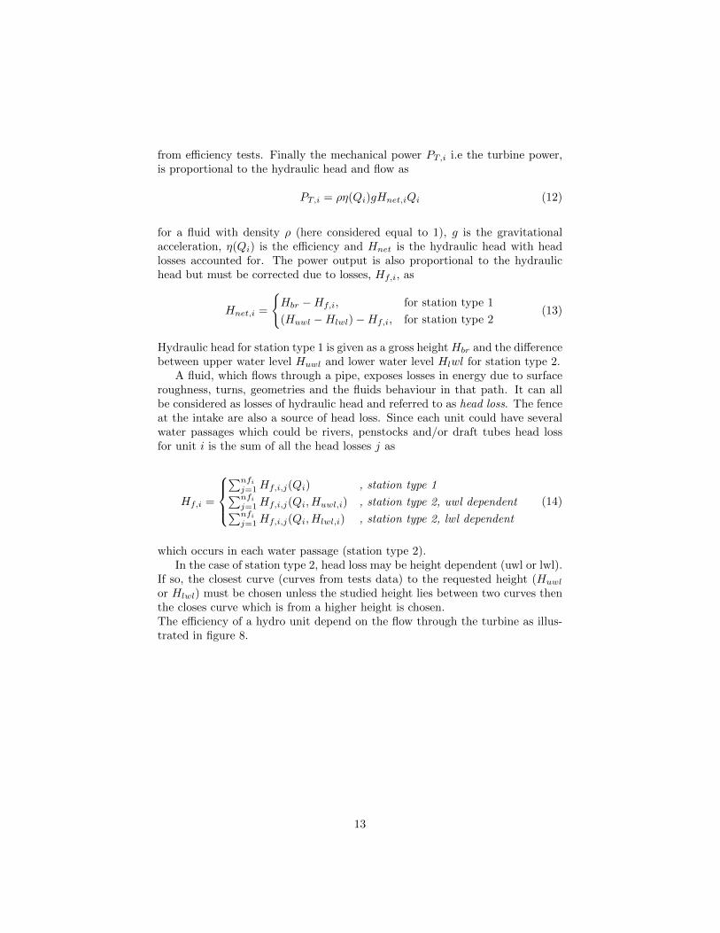
from efficiency tests. Finally the mechanical power PT,i i.e the turbine power,is proportional to the hydraulic head and flow as

PT,i = ρη(Qi)gHnet,iQi (12)

for a fluid with density ρ (here considered equal to 1), g is the gravitationalacceleration, η(Qi) is the efficiency and Hnet is the hydraulic head with headlosses accounted for. The power output is also proportional to the hydraulichead but must be corrected due to losses, Hf,i, as

Hnet,i =

{Hbr −Hf,i, for station type 1

(Huwl −Hlwl)−Hf,i, for station type 2(13)

Hydraulic head for station type 1 is given as a gross height Hbr and the differencebetween upper water level Huwl and lower water level Hlwl for station type 2.

A fluid, which flows through a pipe, exposes losses in energy due to surfaceroughness, turns, geometries and the fluids behaviour in that path. It can allbe considered as losses of hydraulic head and referred to as head loss. The fenceat the intake are also a source of head loss. Since each unit could have severalwater passages which could be rivers, penstocks and/or draft tubes head lossfor unit i is the sum of all the head losses j as

Hf,i =

∑nfij=1Hf,i,j(Qi) , station type 1∑nfij=1Hf,i,j(Qi, Huwl,i) , station type 2, uwl dependent∑nfij=1Hf,i,j(Qi, Hlwl,i) , station type 2, lwl dependent

(14)

which occurs in each water passage (station type 2).In the case of station type 2, head loss may be height dependent (uwl or lwl).

If so, the closest curve (curves from tests data) to the requested height (Huwl

or Hlwl) must be chosen unless the studied height lies between two curves thenthe closes curve which is from a higher height is chosen.The efficiency of a hydro unit depend on the flow through the turbine as illus-trated in figure 8.

13

Figure 8: Hill-diagram of efficiency versus volumetric flow rate for a given netheight. Retrieved from [13].

The efficiency is also dependent on the net height. Efficiencies at differentheights is gathered (nominal heights), and to estimate efficiency values in theregions outside the known lines, interpolation or extrapolation is used. Forvalues between the curves, linear interpolation is used.

For a studied net height that lies between two efficiency curves in terms oftheir respective nominal heights, green and red area in figure 9, the efficiency isthen linearly interpolated.

14

Figure 9: Efficiency dependent on head and flow is calculated in different ways.It is either interpolated between two curves or extrapolated using incompress-ibility equation.

In the green area

ηi(Hnet,i) = ηHnom,1 +ηHnom,1 − ηHnom,2Hnom,1 −Hnom,2

(Hnet,i −Hnom,1

). (15)

is used. In the case of the red area, where one of the curve is too short, in-terpolation will be done from the shorter curve to the longer curve graduallyskewed until both ends are reached and interpolation is done between the twoend points. Gradually skewing interpolation is done with

Pkn = 1− Hnom,1

Hnet,i(16)

pk =Hnom,2 −Hnet,i

PknHnet,i(17)

∆Qk = Qi −Qmax,1 (18)

∆QL = Pk∆Qk (19)

Qakt,2 = Qi + ∆QL (20)

Qakt,1 = Qmax,1 (21)

15

and if Qakt,2 > Qmax,2 then Qakt,2 is corrected using

∆Qut =(Qak,2 −Qmax,2)Hnet,i

Hnet,i −Hnom,i(22)

Qakt,1 = Qmax,1 + ∆Qut (23)

Qakt,2 = Qmax,2 + ∆Qut. (24)

Efficiency is then calculated using cubic splines with Qakt,1 and Qakt,2 as inputparameters and interpolated for Hnet,i in Hnom,1 < Hnet,i < Hnom,2.

Polynomials together with breakpoints to form cubic splines, f(x), are widelyused to calculate several factors with respect to input parameters, x. For the ef-ficiency and guide vane angle of attack f(x) corresponds to η(Qi) and A0i(PT,i)respectively.

Equations 16 through 24 is altered to fit problems were either ηHnom,1 islonger than ηHnom,2 or the other way around.

If the head lies in the blue area in figure 9 above or below a measuredefficiency at nominal height Hnom,i the incompressibility equation is used toextrapolate the nominal flow as

Qnom,i = Qi

√Hnom,i

Hnet,i(25)

which is then used to calculate the efficiency using the cubic splines where f(x)now corresponds to η(Qnom,i).

3.3 Problem setup

The objective is to find the best combination flows Q1, Q2, Q3, ..., Qn betweenthe active hydro power plant units which maximizes the power output of thepower plant as

max(P (S,H,Qtot, Q1, Q2, ..., Qn)) (26)

where S is the active unit combination, H is the head, Qtot is the total flow.The active unit combinations can only be represented as a discrete value makingthe problem which makes the objective problem formulation a mixed integernonlinear programming problem. By computing the optimal flow distributionfor all the combinations, nS , requested heights and total flow the problem thenbecomes a nonlinear problem. The optimization problem must also satisfy thereal-world restrictions and limitations as

16

max(P (Q1, Q2, ..., Qn)) (27)

s.t. Qtot =

n∑i

Qi +

m∑k

Qleakage,k (28)

Qmin,i ≤ Q ≤ Qmax,i. (29)

The problem is constrained by equality constraint 28 which states that totalwater flow through the hydro power plant is the sum of all the flows throughactive units and the leakage of the inactive units. The simple bounds 29 aregoverned by the allowed water flow through each turbine.

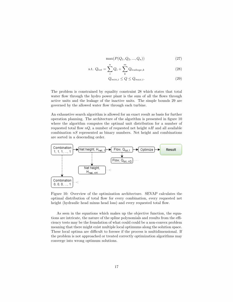
An exhaustive search algorithm is allowed for an exact result as basis for furtheroperation planning. The architecture of the algorithm is presented in figure 10where the algorithm computes the optimal unit distribution for a number ofrequested total flow nQ, a number of requested net height nH and all availablecombination nS represented as binary numbers. Net height and combinationsare sorted in a descending order.

Figure 10: Overview of the optimization architecture. SEVAP calculates theoptimal distribution of total flow for every combination, every requested netheight (hydraulic head minus head loss) and every requested total flow.

As seen in the equations which makes up the objective function, the equa-tions are intricate, the nature of the spline polynomials and results from the effi-ciency tests may be the foundation of what could could be a non-convex problemmeaning that there might exist multiple local optimums along the solution space.These local optima are difficult to foresee if the process is multidimensional. Ifthe problem is not approached or treated correctly optimization algorithms mayconverge into wrong optimum solutions.

17

3.4 Optimization algorithm: initial point

To ensure that SEVAP will reach the best local optimum as possible optimizingequation 27 through 29, three strategies are used to generate three differentinitial guesses where the optimization algorithm starts from.

3.4.1 Strategy 1

Strategy number one works by prioritizing the unit which allows smallest flowsby maximizing its flow while making sure the other units stay within acceptedflows. When the first unit is maximized the next unit with the second lowestallowed flow is maximized until all they units are maxed out. This strategystates that low flow results in low efficiency.

3.4.2 Strategy 2

Strategy number two is based on the previous calculated optimum (previoustotal flow if previous total flow exist) by adding flow proportional to that pointto make sure the sum of the new start point is equal to the total flow throughthe power plant as

∆Q = Qtot,k −Qtot,k−1, (30)

Qk = Qk−1

(1 +

∆Q∑ni Qi,k−1

), (31)

for total flow and distributed flow number k. This strategy assumes that thenext optimum would lie close to the previous optimum.

3.4.3 Strategy 3

Strategy three distributes the flow over the active units proportionally withrespect to each maximum allowed flow by

∆Q = Qtot,k −Qtot,k−1 (32)

Q = Qk−1 + ∆QQmax −Qmin∑n

i (Qmax,i −Qmin,i). (33)

For a two or three dimensional problem this could be considered as the diag-onal of the rectangle/cuboid which makes up the solution space. This strategymakes sure that even if strategy one and two get stuck in local optimum on oneside of the ”diagonal” of the solution space strategy three may introduce newoptimums.

18

3.4.4 Peps-factor

The result of each optimization is compared to the results from the previouschosen strategy and a factor Peps [MW ], which is specified for each powerplant (typically 0.2% of maximum power output), to ensure a smooth transitionbetween strategies as possible as total flow Qtot changes. For the first flowSEVAP will always chose strategy number 1 and for the rest of the flows SEVAPwill choose according to the flow chart in figure 11.

Figure 11: Schematic overview of how to choose between the initial guessstrategies accounting for the Peps factor for a smooth transition between thedistributions given previous chosen strategy was strategy 1. Results from allthe strategies are compared.

Without the Peps factor, one strategy may find an optimum with a distribu-tion Q which is the complete opposite in terms of flow distribution of the unitsof another strategy which may be the better solution for the next step but thegain of power may be very small due to the nature of the objective functionor even numerical errors. This could result in unnecessary switching betweenthe units and lead to an increased wear of the units. An example of a two unitpower plant would be going from a distribution of 20/80 % of total flow to 80/20% for a small increase in power in proportion to the power output

3.5 Production efficiencies

The theoretical available power output is calculated using the gravitational con-stant g, hydraulic head H and the total flow Qtot as

Pnat = gρHQtot (34)

19

for no head loss and 100% efficiency. Power loss Pf can be calculated as thedifference between theoretical power and actual power output as

Pf = Pnat − P. (35)

The total plant efficiency is described as the fraction between actual poweroutput and the theoretical available output

ηplant =P

Pnat.. (36)

The relative efficiency scales the efficiency according to the inverse of its highestefficiency which ensure it peaks at 1 as

ηrelative(Qi, H, S) =ηplant(Qi, H, S)

max(ηplant(H)

) (37)

Limited efficiency is defined as differentiating the power output of the powerplant with respect to the total flow and offsetting the curve likewise the relativeefficiency as

ηlimited =dP

dQtot· 1

max(ηplant(H)

) . (38)

20

4 Method

4.1 SEVAP architecture

The main goal of this project was to implement the new SEVAP into MATLAB.The architecture of SEVAP system is presented in figure 12.

Figure 12: General flow chart of the optimization process from efficiency testdata to data for operation planning.

Optimization of a hydro power plants starts by performing so called index tests,i.e. experimental efficiency tests on said plant gathering data points. Eachunits characteristics are examined finding point data for ηi(Qi), A0i(PT,i) andgenerator- and transformer efficiency as well as leakages as the nominal hy-draulic head Hnom,i is noted for extrapolation and/or interpolation accordingly.The network of penstocks and draft tubes are examined in terms of their con-nections and intersections to figure out how the water enters and leaves eachunit to find the losses of said units. The head loss Hf,i(Qi) is noted at a specificheight be it Huwl,i, hlwl,i or Hnom,i. Head loss of the river is examined the sameway as the penstocks and draft tubes. The power plant is also studied in termsof if the efficiency and/or head loss is dependent on the water levels and noted

21

accordingly. This could be due to geometries in the outflow, river upstream anddownstream or due to a wide range of operating hydraulic heads.

The characteristics of the hydro power plant and its setup is compiled intoseparate files. Once the data points are stored in separate files, SEVAP will im-port the files to fit polynomials to the data points. For this cubic splines are usedto obtain continuous derivatives, a prerequisites for gradient-based optimizationmethods.

Using the polynomial splines data, SEVAP can produce what is called theQP-table which describes flow Qi, turbine output power PT,i and guide vanesettings A0,i for each unit and net height.

SEVAP now have what is needed to start the optimization but must firstcheck if the power plant is a station type 1 or 2.

In the case of a station type 1 the optimization is done and SEVAP outputs theresult in a table displaying unit distributions for each requested total flow, grossheight and combination. The three efficiencies from equation 36 through 38 isthen calculated and plotted for all heights and combination. The same goesfor station type 2 but instead of gross height the table displays uwl and lwl.Station type 2 will also do what is called a system for operation optimization orSOPT for short. SOPT examines the results from the optimization and picksout the best combination for all the requested flows for a given combination ofuwl and lwl which resembles the envelope of the optimization.

Circled in red in figure 12 is a Quasi-SOPT which is made for comparisononly and will not be implemented in the new SEVAP.

4.2 Software

MATLAB has a wide variety of pre-built functions and toolboxes (extensions)which can be implemented which has been thoroughly tested and consideredreliable. Some of which are for local and/or global optimization for constrainedand unconstrained problems ready to be used. While the global optimizationalgorithms is build to find the global optimum, a good set of starting pointstrategies (based on knowing the problem) along with a local optimization al-gorithm is often faster and may even converge to the same optimum as theglobal algorithm.

4.2.1 Local optimization

The current version of SEVAP uses the iterative search method optimizationengine VE03 written by the HSL group [14] in Fortran 77. VE03 finds theminimum of a general function f(x) of n variables x1, x2, ..., xn subject to simplebounds and linear constraints suits this optimization problem. The optimizationengine calls a subroutine to calculate the objective function f(x) and a vectorof the first derivatives δf

δxi. If the problem turns out to be too difficult to find

its derivative the user may have to do some approximation and simplifications

22

which may lead to uncertainties in the representation of objective function. TheHSL group then recommends the user to find the first derivative numericallyusing the finite difference method

δf

δx=f(x + he1)− f(x)

h(39)

where e1 is the vector (1, 0, 0, ..., 0) and so on and small h. However, thisnumerical derivation has not been implemented by Vattenfall in Fortran in thecurrent version.

The optimization toolbox in Matlab has a local optimization solver calledfmincon() which is an iterative search algorithm. Just as VE03 fmincon is agradient based method which minimizes constrained continuous problems withsimple bounds and have a continuous first derivative but does require the firstderivative as an input [11].

4.2.2 Global optimization

The global optimization toolbox in Matlab has a few build-in algorithms forfinding the global optimum of a constrained problem with simple bounds, glob-alsearch(), multistart() and particleswarm(). Both global search and multi startare based on the fmincon algorithm for convergence but has different approachesfor choosing a start point. Global search perform a local convergence from astarting point x0 and generates trial points based on the converged point whichare evaluated if their suitable as starting points in advance. The result from thestarting points are then compared for the best result. Multi start uses a morestraight forward brute force method where it will generate multiple startingpoints and converge from there and finally evaluate the results. Particle swarmis a population based algorithm similar to that of a genetic algorithm which doesnot require starting point. A number of particles are generated which movesin steps in the region evaluating the objective function at each step and thendecide upon a new direction and step size. Each particle tends towards its bestlocation as well as the flocks best location found.

Previous results using the old version of SEVAP running VE03 with thethree strategies will be compared to the results from fmincon() using the samethree strategies and the results from globalsearch() as well as particleswarm()and be evaluated in terms of its run time. As this master thesis project wasdone parts with Jonas Almgrund the study and results of different optimizationalgorithms can be found in his report on alternative optimization algorithms forhydro power plants [21].

4.3 Testing and validation

For validating the new implemented SEVAP three hydro power plants (out ofVattenfalls many power plants) was chosen for test. The chosen power plants willbe remained anonymous with pseudonyms and input data will not be presented

23

in this report due to security reasons and trade secrets. Numerical results willalso be hidden for the same reason. The three chosen power plants are presentedin table 1 with each number of units and size.

Table 1: Hydro power plants tested with the new verison of SEVAP.

Power plant No. units Size Water level dependent

Nattan 1 small unit and head lossMellerdrag station 3 medium no

Rakneforsen kraftverk 6 medium/large no

Nattan has three water level dependent unit file for its one unit and two headlosses with one consisting of three water level dependent files. Mellerdrag hasone unit file per unit and four head loss files. Rakneforsen has one unit file perunit and eight head loss files.

All of the power plants will be calculated as station type 2. The new versionof SEVAP produces the same production planning foundation as the currentversion and the difference between the two versions will be tested by finding thedifference:

• Between current result and new result, Ptot, based on the same distribu-tions Q1, ...Qn, from current version of SEVAP. This validates the object-ive function.

• Between old and new results, Ptot, to tests the optimization tools.

Since the studied power plants are station types 2 the difference will be foundusing the SOPT-tables only for the requested heights. OPT-tables will not becompared due to the large data output from the optimization which rendersvisual representation difficult.

Comparison between the current version of SEVAP can only be done usingfiles which have been outputted and therefore been rounded to three decimalplaces whereas the results from the new SEVAP can be stored in MATLAB andhave a double precision. These difference in precision’s might lead to fluctuationin the difference between the two results.

Production and distribution curves will be presented for just one of thestation due to the large amount of data per station available.

Inaccuracy of testing equipment for index/efficiency test is ±0.3% [20].

24

5 Results

The new SEVAP built in MATLAB does require MATLAB R2018b or laterversion with optimization toolbox installed to run.

The data files that the new SEVAP imports is presented in appendix A andthe new GUI of SEVAP is presented in the appendix B.

5.1 Testing and validation

The one unit hydro power plant Nattan validates the objective function in termsof water level dependence in figure 13. No optimization has been done due thereonly being one unit.

N51P

0 20 40 60 80 100 120 140 160 180 200

Qtot

[m3/s]

0

1

2

P [K

W]

Pcalculated

- PImported

H1

H2

H3

H4

H5

H6

Figure 13: Validation of Nattan.

As seen in figure 13 the difference between power from the six requested heads,H1, ...,H6, calculated from current SEVAP solution and power imported fromSEVAP solution lies around rounding errors. Computation time ≈ 0.02 seconds.

Figure 14 shows the difference between new SEVAP optimization and cur-rent SEVAP optimization as well as the difference between power calculatedfrom current SEVAP solution and power imported from current SEVAP forMellerdrag station.

25

0 100 200 300 400 500 600 700

Qtot

[m3/s]

-50

0

50

100P

[K

W] H

1

H2

H3

H4

0 100 200 300 400 500 600 700

Qtot

[m3/s]

0

2

4 H1

H2

H3

H4

0 100 200 300 400 500 600 700

Qtot

[m3/s]

0

1

2

P [K

W]

Pcalculated

- Pimported H

1

H2

H3

H4

Figure 14: Validation of Mellerdrag station and optimized output power compar-ison between new and current SEVAP for the four requested heights, H1, ...,H4.

Comparison between the optimized output power shows difference around 0 permill with a few exceptions with 4 per mill in the favour of the new optimizationalgorithms. Comparison between calculated and imported is less than 2 kW.Computation and optimization time ≈ 47 seconds.

Optimization results for the six unit hydro power plant Rakneforsen kraftverkis presented in figure 15 as well as validation of power output calculation forthis large set of units and head losses.

26

0 100 200 300 400 500 600 700 800

Qtot

[m3/s]

-200

0

200

P [K

W]

H1

H2

H3

H4

H5

H6

H7

H8

0 100 200 300 400 500 600 700 800

Qtot

[m3/s]

-2

0

2

4

H1

H2

H3

H4

H5

H6

H7

H8

0 100 200 300 400 500 600 700 800

Qtot

[m3/s]

0

0.5

1

P [K

W]

Pcalculated

- Pimported

H1

H2

H3

H4

H5

H6

H7

H8

Figure 15: Validation of Rakneforsen kraftverk and optimized output powercomparison between new and current SEVAP for the requested heights,H1, ...,H8.

The new SEVAP optimized output power proves a better solution in termsof power output P for some flow, Qtot, but has a dip at full capacity of lessthan −0.2% compared to current SEVAP optimization. Validation of the poweroutput calculation shows that difference lies within rounding error proving thenew SEVAP solution. Comparison is in the favour of the new SEVAP if thepower plant is not on full capacity. Optimization and computation time ≈ 32minutes.

5.2 Production results

This section will present production result from the new SEVAP.Optimized distribution based on the SOPT for Rakneforsens kraftverk is

presented in figure 16.

27

0 100 200 300 400 500 600 700

Q [m3/s]

A0

i [%

] A1

A2

A3

A4

A5

A6

(a) Guide vane angle A0i.

0 100 200 300 400 500 600 700

Q [m3/s]

Qi [m

3/s

]

Q1

Q2

Q3

Q4

Q5

Q6

(b) Flow, Qi.

0 100 200 300 400 500 600 700

Q [m3/s]

Pi [

MW

]

P1

P2

P3

P4

P5

P6

(c) Transformer power, Ptr,i.

Figure 16: Distributed variables versus total flow rate for Rakneforsens kraftverkfor one combination of Huwl and Hlwl.

One of the units in Rakneforsens kraftverk shows to be the more favourable unitas optimization allocates production to that unit for most of the steps. Thisunit is also the unit with the highest capacity of this power plant.

Results of the plant efficiency from the optimization, OPT+, for one com-bination of Huwl and Hlwl all the S = 2n− 1, this case S = 63 combinations, ispresented in figure 17 as well as the associated SOPT-curve.

28

0 100 200 300 400 500 600 700

Q [m3/s]

PE

[%

]

(a) OPT+.

0 100 200 300 400 500 600 700

Q [m3/s]

PE

[%

]

(b) SOPT.

Figure 17: Plant efficiency in terms of OPT and SOPT for Rakneforsenskraftverk for one combination of Huwl and Hlwl.

Various step size in Qtot increment in the OPT+ for the different combinationresulted in a lower resolution of the SOPT-curve. A high step size was usedto reduce computation time down to ≈ 32 minutes. The OPT+ figure showsclearly why it is necessary to switch combination. As total flow, Qtot, increases,each combination’s efficiency peaks and then reduces. Each combination’s rangeof operation is also visible in the plot.

29

The limited efficiency (Swedish: gransverkningsgrad) of the OPT+ in figure17a for Rakneforsen kraftverk is presented in figure 18.

0 100 200 300 400 500 600 700

Q [m3/s]

LE

[%

]

Figure 18: Limited efficiency of Rakneforsen kraftverk.

The limited efficiency how sensitive each combination is to change of total flow,Qtot.

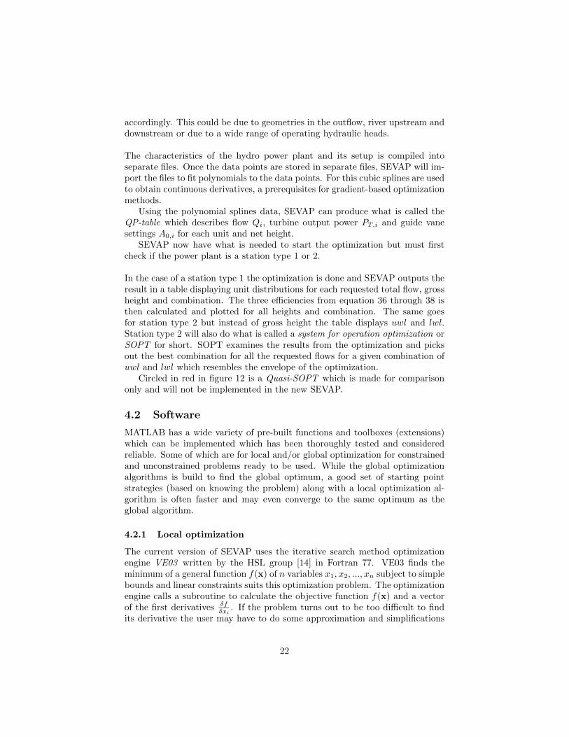
Figure 19 shows the same OPT+ and SOPT as previously presented resultsin terms of power output compared to theoretical power output for the samehydraulic head and flow Qtot.

30

0 100 200 300 400 500 600 700

Q [m3/s]

P [M

W]

Theoretical output

(a) OPT+.

0 100 200 300 400 500 600 700

Q [m3/s]

P [M

W]

Actual output

Theoretical output

(b) SOPT.

Figure 19: Power output from OPT+ and SOPT for Rakneforsens kraftverk forone combination of Huwl and Hlwl.

Figure 19 shows actual power output in relation to theoretical power outputwhich together with 17 shows the characteristics of this power plant and thebig dip towards higher flow. With values along the Y-axis of the SOPT-curve,market department of Vattenfall can match electric power generated from eachpower plant to demand.

31

5.3 Limitation

The current SEVAP has been fitted with functionalities to handle specific hydropower plants with a more intricate design. One of which is Harspranget wherethe draft tubes are interconnected affecting the flow in each draft tube dueto flow distribution. These exceptions have not been implemented in the newversion of SEVAP.

Due to limited work time not all of Vattenfall’s hydro power plants have beentested in the new version of SEVAP to verify the reliability of the new SEVAP.Functions for post processing the results from the optimization and SOPT havebeen written but not implemented in the new version of SEVAP GUI and mustbe run manually in the MATLAB command window.

32

6 Discussion and conclusions

6.1 Discussion

Validation of the three chosen power plants proved that the new SEVAP couldindeed compute the correct power output within accuracy of the measurementsand rounding. Some fluctuation did occur which might also be due to truncationand numerical errors or even the modelling of the power output. Although, onecannot draw the conclusion that the function for calculating the power outputis accurate before thoroughly testing it with more of Vattenfalls hydro powerplants and comparing it with current SEVAP results to ensure that the marketdepartment receives correct data for production planning.

This thesis did not study different types of algorithms such as algorithmspecified for finding global optima which in terms could lead to an even bet-ter solution and therefore higher income than what is currently implemented orwhat this thesis suggests. The method used was a combination of brute force forcombinatorial optimization and then a gradient based optimization algorithmfor optimizing the objective function for handling the mixed integer nonlinearproblem. As the computation and optimization times are not specified as scarceresource one could even consider utilizing brute force for finding an optimal solu-tion for the objective function. This would be done by computing the poweroutput with multiple discrete steps of Q1, ...Qn. Resolution of the steps usedfor this brute force would effect the optimization run-time and tolerance of thesolution. However in reality brute force method will most likely consume toomuch time and might not be considered a liable option.

As of now Peps works as a hard limit. If Peps = 0.2 MW and a strategyresults in a power increase of 0.19 MW, the new strategy and its solution willbe ignored no matter the distance to the previous distribution. A switch from20/80 to 80/20 is treated the same as switching from 20/80 to 22/78.

6.2 Conclusion

The main conclusion of this work are:

• The MATLAB implementation of SEVAP reached the same results asthe current FORTRAN 77 based version down to rounding errors andmeasurement inaccuracies.

• The computational time for the MATLAB implementation of SEVAP ismuch longer compared to the FORTRAN implementation of SEVAP. Thisis, however, no big disadvantage since the optimizations are done offlineand are not time critical.

• The new implementation of SEVAP is more flexible and easily integratedwith future projects for further development.

33

6.3 Future work

The Peps-factor is a hard coded value for each power plant (based on total poweroutput) but could instead be implemented in the objective function as a pen-alty for moving further away from the distribution in the previous Qtot valueoptimized for. This would ensure a smooth transition while not skipping bettersolutions close to the previous solution distribution.

As of writing this thesis, the layout of the output files are based on the con-strained output format from punch cards. This could be modernised and easethe workability. This project completed the implementation of optimization(OPT, OPT+ and SOPT) part of SEVAP for the standard power plants andoutputs files with the correct format but further work might include reformat-ting the output data files.

The new SEVAP optimizes for a range of Qtot starting from the sum of act-ive unit’s

∑ni Qmin,i ≤ Qtot ≤

∑ni Qmax,i but upon presenting the progress of

this work Vattenfall presented the need of reformulating the range in terms ofmaximum and minimum allowed power output, Pmin and Pmax. An option toreformulate the problem in terms of minimize water usage for a given power out-put could also be implemented. Implementation of this at market using SEVAPsresults could lead to a lower resolution and rounding errors could occur.

As of writing this thesis the new SEVAP require that the user runs the programthrough MATLAB. If the program were to be compiled into an executable pro-gram based on machine code computational time would be reduced drasticallyand the user will no longer need to understand the MATLAB UI. Although,this cannot be done for the optimization toolbox. Parallel computing toolboxcould also be implemented to reduce computational time even more.

The GUI developed was not the main focus of this work and may come tochange as Vattenfall now has the MATLAB functions for computing power out-put and optimizing power plants.

34

References

[1] Elens ursprung och miljopaverkan - Vattenfall. (2019). Retrieved fromhttps://www.vattenfall.se/elavtal/energikallor/elens-ursprung/

[2] Statens energimyndighet. (2014). Vad avgor ett vattenkraftverks betydelsefor elsystemet. Eskilstuna.

[3] Byman, K., Koebe, C. (2016). Sveriges framtida elproduktion. Stockholm:Kungl. Ingenjorsvetenskapsakademien (IVA).

[4] Molin, J., Andersson, H. (2016). Vattenkraft. Retrieved fromhttp://www.energimyndigheten.se/fornybart/vattenkraft/

[5] Sa fungerar vattenkraftverk - Vattenfall. (2019). Re-trieved from https://corporate.vattenfall.se/om-energi/el-och-varmeproduktion/vattenkraft/sa-fungerar-vattenkraft/

[6] File:Water turbine (en).svg - Wikimedia Commons. (2008). Retrieved fromhttps://commons.wikimedia.org/wiki/File:Water_turbine_(en).svg

[7] J. lundgren, M. Ronnqvist, P. Varbrand. Linjar och icke-linjar optimering.Lund: Studentlitteratur, 2001

[8] Vattenfall. (December, 2012) Rekordar for vattenkraften[Online].https://corporate.vattenfall.se/press-och-media/nyheter/

import-nyheter/rekordar-for-vattenkraften/. [Accessed 11 Feb.,2019].

[9] Vattenfall. (2009, July) Fordelar och nackdelar med olika kraftslag[Online].https://corporate.vattenfall.se/press-och-media/nyheter/

import-nyheter/fordelar-och-nackdelar-med-olika-kraftslag/.[Accessed 11 Feb., 2019].

[10] Von Klopp, H. (2011). Naverede. Retrieved from http://www.vonklopp.

se/wordpress/?p=2671.

[11] Find minimum of constrained nonlinear multivariable function - MATLABfmincon- MathWorks Nordic. Retrieved from https://se.mathworks.com/

help/optim/ug/fmincon.html#busp5fq-6

[12] Dahlin. J. [BINDER] SEVAP optimization, PY-OM - Vattenfall Vatten-kraft AB.

[13] Finardi, E., Silva, E., Sagastizabal, C. (2005). Solving the unit commit-ment problem of hydropower plants via Lagrangian Relaxation and Sequen-tial Quadratic Programming. Computational Applied Mathematics, 24(3).doi: 10.1590/s0101-82052005000300001

[14] (2011). Retrieved from http://www.hsl.rl.ac.uk/archive/specs/

ve03.pdf

35

[15] Bortoni, E., Bastos, G., Abreu, T. and Kawkabani, B. (2015). Optimalpower distribution between units of a hydro power plant. Renewable Energy,75, p.536.

[16] (Lecture notes)CSC 8301 - Design and Analysis of Algorithms. (2017).

[17] Siu, T., Nash, G. and Shawwash, Z. (2001). A practical hydro, dynamicunit commitment and loading model. IEEE Transactions on Power Systems,16(2).

[18] Finardi, E. and da Silva, E. (2005). UNIT COMMITMENT OF SINGLEHYDROELECTRIC PLANT. Electric Power Systems Research, 75(2-3),pp.116-123.

[19] Cristian Finardi, E. and Reolon Scuzziato, M. (2013). Hydro unit commit-ment and loading problem for day-ahead operation planning problem. Inter-national Journal of Electrical Power & Energy Systems, 44(1), pp.7-16.

[20] Kraftkonsult. (2009-01-30) Produktionsekonomi i Vattenkraftanlaggningar- Anlaggningsprov och utvardering.

[21] Almgrund, J. (2019). Alternative Methods for Operational Optimiza-tion of Hydro Power Plants, Unpublished manuscript, Kungliga TekniskaHogskolan, Stockholm.

36

A Data files

The new SEVAP software works by importing the same data files from theindex/efficiency tests as current SEVAP imports. The data is split into threefiles; unit, head loss and a station file. Figure 20 shows the layout of the unitfiles. The data is represented in ASCII format in ’.txt’ files and the first columnis used to identify what data is stored in each row and first row is always theheader which stores general information.

Figure 20: Input data file format for unit No. i (Gi) for plant Nattan.

First row, T, stores the shorted station name, unit number i, at which heightthis data was gathered, leakage at guide vane angle 0◦, minimum and maximumallowed flow through the unit. Rows P and A are measured data points ofthe mechanical power (PT ) with respect to guide vane angle. Rows Q and Vholds the data points for flow and efficiency of the unit. Row X and Z arethe weights for the data points for the spline fitting. Row B and D are thebreak points for A0i(PT ) and ηi(Qi) respectively for the spline fitting whichgenerates coefficients stored on rows K1,K2, ...,Kb and M1,M2, ...,Md. RowE and G holds the date of spline fitting, root mean square error, maximumdeviation of the spline fittings. Maximum efficiency and the flow responsible forthis efficiency is presented in row G.

Layout of the head loss data file is presented in figure 21.

Figure 21: Input data file format for head loss for water passage No. j.

The first row, F, holds the shortened name, which water passage, j, is rep-resented. In the case of water level dependence head loss the specified Huwl

or Hlwl is presented in the header dependent on which dependence the waterpassage has which is presented in the station file. This position is left empty ifthe head loss is not dependent on the water level. Rows Q and H stores themeasured data of Qi(Hf,j). Row B holds the break points for the cubic splineswhich generates the coefficients stored in the rows K1,K2, ...,Kb. Row E storesthe date which the spline fitting was performed, root mean square error andmaximum deviation of the spline fitting.

There are no difference between station type 1 and 2 for the unit and headloss files but there exist differences in the station files as seen in figure 22.

(a) Station type 1, NA54. (b) Station type 2, NA54P.

Figure 22: Input data files (NA54/NA54P) for power plant Nattan.

The header contains the full name of the power plant as well as the shortenedname, station number, number of units, number of water passages, routinedirective for computing the head loss and the Peps-factor. Number of unitsand number of water passages must have minimum one data file each. Rowsstarting with M represents which head loss file applies to which water passageusing a binary combination. If a station has 3 units and head loss file 1 appliesto number 2 and 3, M1 will then be 0, 1, 1. Row N stores the net heights usedto calculate the QP-table. For station type 1 there exists a row B which holdsthe gross heights which are the gross heights used for optimization. For stationtype 2 row Y holds the upper and lower water levels for the optimization andSOPT results. The coefficients for calculating the generator and transformersefficiency is stored in row G for each unit as ai1, ai2, ai3 and bi1, bi2, bi3. If thereexist water level dependent head losses (only station type 2) it is represented inthe rows F for water passages j and weather it is dependent on the Huwl or theHlwl with a number 1 or 2.

Each power plant stores its data files in a folder named after it shortenedname (one for station type 1 and 2).

B New SEVAP GUI

The GUI of the new SEVAP is presented in 23

Figure 23: GUI of the new SEVAP.

By assigning the directory to the input files in options all the power plantsdata folders is listed in table circled in red as number 1 in the GUI. By clickingon one of the power plants, all its data files appear in the table circled as number

2. Curve fitting is done by choosing a data file (unit or head loss) and by clickingthe button Calculate which is circled as number 3. Window 6 and 7 presentsthe results from the polynomial fitting for post processing. Once all the curvefittings are done the user may enter the Qtot step size for each combination inthe table circled 4 for the optimization. If there exists a directory file withsaved desired step sizes it is automatically filled in the table when choosing thepower plant in table circled 1. If not, default value is set to 10. Resolutionfor the SOPT file must also be assigned. Default value is set to the maximumstep size for the optimization if no other value is set by the user. Optimizationcan be done by pressing the button ”Optimization” circled as number 8. Notyet implemented in the GUI are the production plots but they are ploted inseparate windows.

The program automatically generates files storing the OPT/OPT+ andSOPT files in the same format as the current SEVAP (based on a constrainedpunch card formatting) to ensure market department can utilize the result fromthe optimization. OPT and OPT+ files consists of a header with active units,maximum and minimum flows, Hbr (OPT) or Huwl and Hlwl (OPT+), dateof optimization. Below the header is the total flow and power output as wellas each distribution of flow, power output and guide vane angle of active units.This repeats for all active unit combinations and heights. SOPT files are format-ted with a header like that of the OPT+ but outputs all the distribution of allthe units which only needs to repeat for all the heights.