25
Implementation of the Black, Derman and Toy Model Seminar Financial Engineering o.Univ.-Prof. Dr. Engelbert J. Dockner University of Vienna Summer Term 2003 Christoph Klose Li Chang Yuan
Implementation of the Black, Derman and Toy Model
Seminar Financial Engineering o.Univ.-Prof. Dr. Engelbert J. Dockner
University of Vienna Summer Term 2003
Christoph Klose Li Chang Yuan
Implementation of the Black, Derman and Toy Model Page 2
Contents of this paper Contents of this paper....................................... 2 1. Introduction to Term Structure Models..................... 3 2. Term Structure Equation for Continuous Time............... 4 3. Overview - Basic Processes of One-Factor Models........... 7 4. The Black Derman and Toy Model (BDT)...................... 8 4.1. Characteristics......................................... 8 4.2. Modeling of an “artificial” Short-Rate Process.......... 9
Valuing Options on Treasury Bonds ....................... 13 4.3. The BDT-Model and Reality.............................. 16 5. Implementation and Application of the BDT-Model.......... 19 6. List of Symbols and Abbreviations........................ 23 7. References............................................... 24 8. Suggestions for further reading.......................... 25
Implementation of the Black, Derman and Toy Model Page 3
1. Introduction to Term Structure Models
Interest rate derivatives are instruments that are in some way
contingent on interest rates (bonds, swaps or just simple
loans that start at a future point in time). Such securities
are extremely important because almost every financial
transaction is exposed to interest rate risk – and interest
rate derivatives provide the means for controlling this risk.
In addition, same as with other derivative securities,
interest rate derivatives may also be used to enhance the
performance of investment portfolios. The interesting and
crucial question is what are these instruments worth on the
market and how can they be priced.
In analogy to stock options, interest rate derivatives depend
on their underlying, i.e. the interest rate. Bond prices
depend on the movement of interest rates, so do bond options.
The question of pricing contingent claims on interest rates
comes down to the question of how the underlying can be
modeled. Future values are uncertain, but with the help of
stochastic models it is possible to get information about
possible interest rates. The tool needed is the term structure
– the evolution of spot rates over time. One has to consider
both, the term structure of interest rates and the term
structure of interest rate volatilities. Term structure models,
also known as yield curve models, describe the probabilistic
behavior of all rates. They are more complicated than models
used to describe a stock price or an exchange rate. This is
because they are concerned with movements in an entire yield
curve – not with changes to a single variable. As time passes,
the individual interest rates in the term structure change. In
addition, the shape of the curve itself is liable to change.
We have to distinguish between equilibrium models and no-
arbitrage models. In an equilibrium model the initial term
structure is an output from the model, in a no-arbitrage model
Implementation of the Black, Derman and Toy Model Page 4 it is an input to the model. Equilibrium models usually start
with the assumption about economic variables and derive a
process for the short-term risk-free rate r.1 They then explore
what the process implies for bond prices and option prices.
The disadvantage of equilibrium models is that they do not
automatically fit today’s term structure. No-arbitrage models
are designed to be exactly consistent with today’s term
structure. The idea is based on the risk-neutral pricing
formula when a bond is valued over a single period of time
with binominal lattice.
2. Term Structure Equation for Continuous Time
In our paper we prefer to use discrete time models, because
the data available is always in discrete form and easier to
compute. The continues time models do not provide us with
useful solutions in the BDT world2, nevertheless they are the
fundamental and older part of interest rate derivatives.
Continuous time models are more transparent and give a better
understanding of the BDT model, therefore we here give a short
general introduction into this material.
We assume that the following term structure equation3 is given:
( ) ( ) ( ) 0, 221, =⋅−⋅⋅+⋅+ Π trPrtPrtPP rrrt σµ
with
tP
Pt∂
∂= ;
rP
Pr∂
∂= ;
r
PPrr
∂
∂= 2
2
We have a second order partial differential equation. It is of
course of great importance that the partial differential
1 When r(t) is the only source of uncertainty for the term structure, the short rate is modeled by One-Factor Models. 2 The continuous time models can lead to closed form mathematical solutions. But in the BDT case, we cannot find such a solution. 3 Rudolf (2000) pp.38-40
Implementation of the Black, Derman and Toy Model Page 5 equation above leads to solutions for interest derivatives.
Not every Ito process can solve the term structure above.
It turns out that some Ito processes which are affine term
structure models lead to a solution.
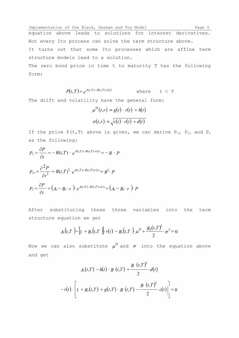
The zero bond price in time t to maturity T has the following
form:
( ) ( )eTtP trTtBTtA ⋅−= ),(),(, where t < T
The drift and volatility have the general form:
( ) ( ) ( ) ( )thtrtgrt +⋅≡Π ,µ
( ) ( ) ( ) ( )tdtrtcrt +⋅≡,σ
If the price P(t,T) above is given, we can derive Pr, Prr and Pt
as the following:
PBeTtBtP
P trTtBTtAr ⋅−=⋅−=
∂
∂= ⋅− )(),(),(),(
PBeTtBr
PP trTtBTtA
rr ⋅=⋅=∂
∂= ⋅− 2)(),(),(2
2 ),(2
( ) ( ) PrBAerBAtP
P tttrTtBTtA
ttt ⋅⋅−=⋅⋅−=∂
∂= ⋅− )(),(),(
After substituting these three variables into the term
structure equation we get
( ) ( )[ ] ( ) ( ) ( )0
2,
,,1, 22
=⋅+⋅−⋅+− Π σµTtBtTtBtrTtBTtA ttt
Now we can also substitute µΠ and σ into the equation above
and get
( ) ( ) ( )( )
( )tdTtB
TtBthTtAt ⋅+⋅−2
,,,
2
( ) ( ) ( ) ( )( )
( ) 02
,,,,1
2
=
⋅−⋅++⋅− tc
TtBTtBTtgTtBtr t
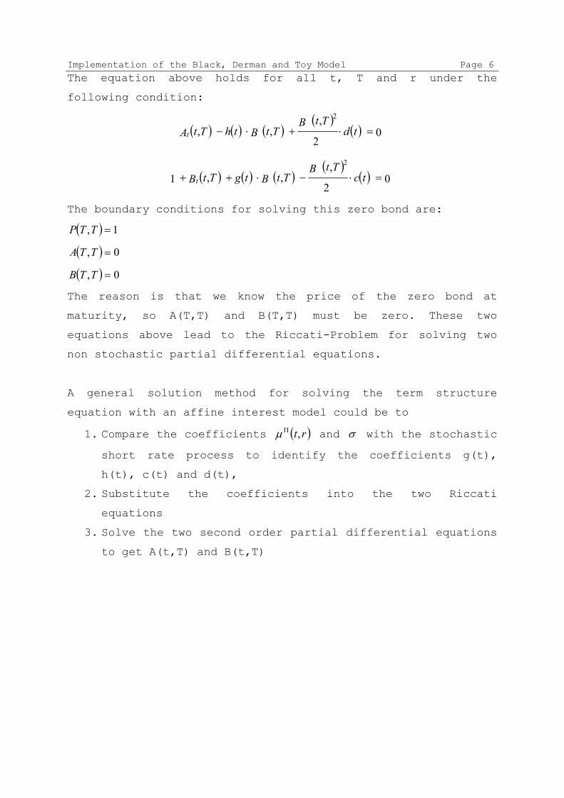
Implementation of the Black, Derman and Toy Model Page 6 The equation above holds for all t, T and r under the
following condition:
( ) ( ) ( )( )
( ) 02
,,,
2
=⋅+⋅− tdTtB
TtBthTtAt
( ) ( ) ( )( )
( ) 02
,,,1
2
=⋅−⋅++ tcTtB
TtBtgTtBt
The boundary conditions for solving this zero bond are:
( ) 1, =TTP
( ) 0, =TTA
( ) 0, =TTB
The reason is that we know the price of the zero bond at
maturity, so A(T,T) and B(T,T) must be zero. These two
equations above lead to the Riccati-Problem for solving two
non stochastic partial differential equations.
A general solution method for solving the term structure
equation with an affine interest model could be to
1. Compare the coefficients ( )rt,Πµ and σ with the stochastic
short rate process to identify the coefficients g(t),
h(t), c(t) and d(t),
2. Substitute the coefficients into the two Riccati
equations
3. Solve the two second order partial differential equations
to get A(t,T) and B(t,T)
Implementation of the Black, Derman and Toy Model Page 7
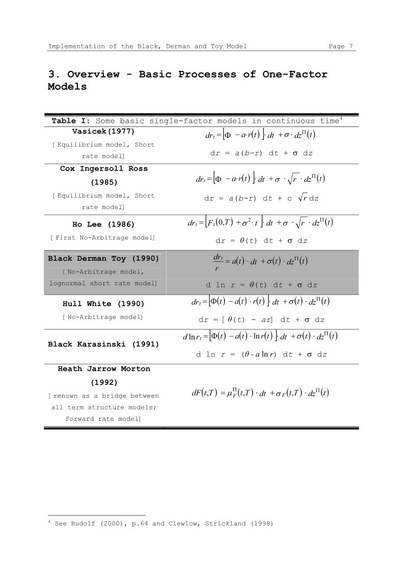
3. Overview - Basic Processes of One-Factor Models
Table I: Some basic single-factor models in continuous time4 Vasicek(1977)
[Equilibrium model, Short
rate model]
( )[ ] ( )tdzdttradrtΠ⋅+⋅⋅−Φ= σ
dr = a(b-r) dt + σ dz
Cox Ingersoll Ross
(1985)
[Equilibrium model, Short
rate model]
( )[ ] ( )tdzrdttradrtΠ⋅⋅+⋅⋅−Φ= σ
dr = a(b-r) dt + c r dz
Ho Lee (1986)
[First No-Arbitrage model]
( )[ ] ( )tdzrdttTFdr ttΠ⋅⋅+⋅⋅+= σσ 2,0
dr = θ(t) dt + σ dz
Black Derman Toy (1990)
[No-Arbitrage model,
lognormal short rate model]
( ) ( ) ( )tdztdttardrt Π⋅+⋅= σ
d ln r = θ(t) dt + σ dz
Hull White (1990)
[No-Arbitrage model]
( ) ( ) ( )[ ] ( ) ( )tdztdttrtatdrtΠ⋅+⋅⋅−Φ= σ
dr = [θ(t) - ar] dt + σ dz
Black Karasinski (1991) ( ) ( ) ( )[ ] ( ) ( )tdztdttrtatrd t
Π⋅+⋅⋅−Φ= σlnln
d ln r = (θ - a ln r) dt + σ dz
Heath Jarrow Morton
(1992)
[renown as a bridge between
all term structure models;
Forward rate model]
( ) ( ) ( ) ( )tdzTtdtTtTtdF FFΠΠ ⋅+⋅= ,,, σµ
4 See Rudolf (2000), p.64 and Clewlow, Strickland (1998)
Implementation of the Black, Derman and Toy Model Page 8
4. The Black Derman and Toy Model (BDT)
4.1. Characteristics The term structure model developed in 1990 by Fischer Black,
Emanuel Derman and William Toy is a yield-based model which
has proved popular with practitioners for valuing interest
rate derivatives such as caps and swaptions etc. The Black,
Derman and Toy model (henceforth BDT model) is a one-factor
short-rate (no-arbitrage) model – all security prices and
rates depend only on a single factor, the short rate – the
annualized one-period interest rate. The current structure of
long rates (yields on zero-coupon Treasury bonds) for various
maturities and their estimated volatilities are used to
construct a tree of possible future short rates. This tree can
then be used to value interest-rate-sensitive securities.
Several assumptions are made for the model to hold:
• Changes in all bond yields are perfectly correlated.
• Expected returns on all securities over one period are
equal.
• The short rates are log-normally distributed
• There exists no taxes or transaction costs.
As with the original Ho and Lee model, the model is developed
algorithmically, describing the evolution of the term
structure in a discrete-time binominal lattice framework.
Although the algorithmic construction is rather opaque with
regard to its assumptions about the evolution of the short
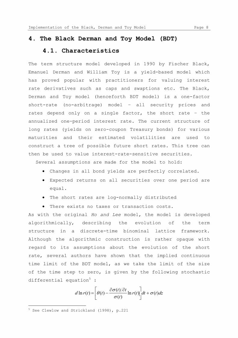
rate, several authors have shown that the implied continuous
time limit of the BDT model, as we take the limit of the size
of the time step to zero, is given by the following stochastic
differential equation5 :
dztdttrt
ttttrd )()(ln
)()(
)()(ln σσσ
θ +
∂∂−=
5 See Clewlow and Strickland (1998), p.221
Implementation of the Black, Derman and Toy Model Page 9 This representation of the model allows to understand the
assumption implicit in the model. The BDT model incorporates
two independent functions of time, θ(t) and σ(t), chosen so
that the model fits the term structure of spot interest rates
and the term structure of spot rate volatilities. In contrast
to the Ho and Lee and Hull and White model, in the BDT
representation the short rates are log-normally distributed;
with the resulting advantage that interest rates cannot become
negative. An unfortunate consequence of the model is that for
certain specifications of the volatility function σ(t) the
short rate can be mean-fleeing rather than mean-reverting. It
is popular among practitioners, partly for the simplicity of
its calibration and partly because of its straightforward
analytic results. The model furthermore has the advantage that
the volatility unit is a percentage, confirming with the
market conventions.
4.2. Modeling of an “artificial” Short-Rate Process In this chapter we describe a model of interest rates that can
be used to value any interest-rate-sensitive security. In
explaining how it works, we concentrate on valuing options on
Treasury bonds. We want to examine how the model works in an
imaginary world in which changes in all bond yields are
perfectly correlated, expected returns on all securities over
one period are equal, short rates at any time are lognormally
distributed and there are neither taxes nor trading costs.
We can value a zero bond of any maturity (providing our tree
of future short rates goes out far enough) using backward
induction. We simply start with the security’s face value at
maturity and find the price at each node earlier by
discounting future prices using the short rate at that node.
The term structure of interest rates is quoted in yields,
rather than prices. Today’s annual yield, y, of the N-zero in
Implementation of the Black, Derman and Toy Model Page 10 terms of its price, S, is given by the y that satisfies the
following equation (1). Similarly the yields (up and down) one
year from now corresponding to the prices Su and Sd are given
by equation (2).
NyS
)1(100+
= (1), 1,
, )1(100
−+= N
dudu y
S (2)
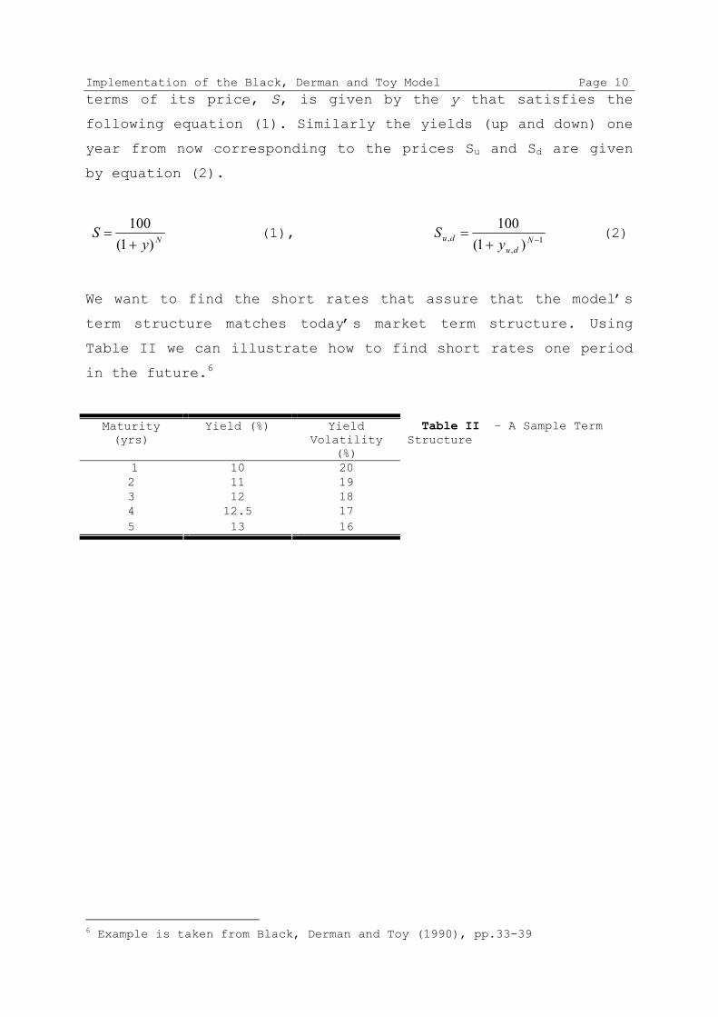
We want to find the short rates that assure that the model’s
term structure matches today’s market term structure. Using
Table II we can illustrate how to find short rates one period
in the future.6
Maturity (yrs)
Yield (%) Yield Volatility
(%) 1 10 20 2 11 19 3 12 18 4 12.5 17 5 13 16
Table II – A Sample Term Structure
6 Example is taken from Black, Derman and Toy (1990), pp.33-39
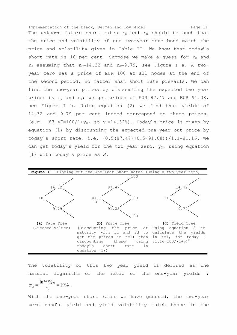
Implementation of the Black, Derman and Toy Model Page 11 The unknown future short rates ru and rd should be such that
the price and volatility of our two-year zero bond match the
price and volatility given in Table II. We know that today’s
short rate is 10 per cent. Suppose we make a guess for ru and
rd assuming that ru=14.32 and rd=9.79, see Figure I a. A two-
year zero has a price of EUR 100 at all nodes at the end of
the second period, no matter what short rate prevails. We can
find the one-year prices by discounting the expected two year
prices by ru and rd; we get prices of EUR 87.47 and EUR 91.08,
see Figure I b. Using equation (2) we find that yields of
14.32 and 9.79 per cent indeed correspond to these prices.
(e.g. 87.47=100/1+yu, so yu=14.32%). Today’s price is given by
equation (1) by discounting the expected one-year out price by
today’s short rate, i.e. (0.5(87.47)+0.5(91.08))/1.1=81.16. We
can get today’s yield for the two year zero, y2, using equation
(1) with today’s price as S.
Figure I – Finding out the One-Year Short Rates (using a two-year zero)
(a) Rate Tree
(Guessed values) (b) Price Tree
(Discounting the price at maturity with ru and rd to get the prices in t=1; then discounting these using today’s short rate in equation (1))
(c) Yield Tree Using equation 2 to calculate the yields in t=1, for today :81.16=100/(1+y)2
The volatility of this two year yield is defined as the
natural logarithm of the ratio of the one-year yields :
%192
ln 79.933.14
2 ==σ .
With the one-year short rates we have guessed, the two-year
zero bond’s yield and yield volatility match those in the
10
9.79
14.32
81.16
91.08
87.47
100
100
100
11
9.79
14.32
Implementation of the Black, Derman and Toy Model Page 12 observed term structure of Table II. This means that our
guesses for ru and rd were right. Had they been wrong, we would
have found the correct ones by trial and error.
So an initial short rate of 10 per cent followed by equally
probable one-year short rates of 14.32 and 9.79 per cent
guarantee that our model matches the first two years of the
term structure.
Implementation of the Black, Derman and Toy Model Page 13
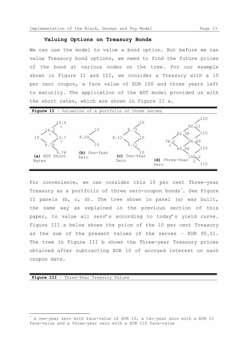
Valuing Options on Treasury Bonds
We can use the model to value a bond option. But before we can
value Treasury bond options, we need to find the future prices
of the bond at various nodes on the tree. For our example
shown in Figure II and III, we consider a Treasury with a 10
per cent coupon, a face value of EUR 100 and three years left
to maturity. The application of the BDT model provided us with
the short rates, which are shown in Figure II a.
Figure II – Valuation of a portfolio of three zeroes
For convenience, we can consider this 10 per cent Three-year
Treasury as a portfolio of three zero-coupon bonds7. See Figure
II panels (b, c, d). The tree shown in panel (a) was built,
the same way as explained in the previous section of this
paper, to value all zero’s according to today’s yield curve.
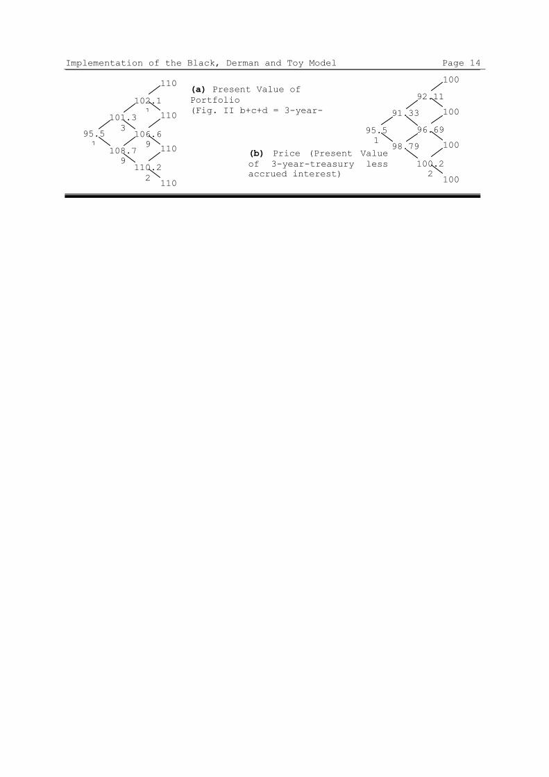
Figure III a below shows the price of the 10 per cent Treasury
as the sum of the present values of the zeroes – EUR 95.51.
The tree in Figure III b shows the Three-year Treasury prices
obtained after subtracting EUR 10 of accrued interest on each
coupon date.
Figure III – Three-Year Treasury Values
7 a one-year zero with face-value of EUR 10, a two-year zero with a EUR 10 face-value and a three-year zero with a EUR 110 face-value
10
14.32
9.79
19.42
13.77
9.76
9.09
10
10
8.12
8.75
9.11
10
10
10
78.30
82.58
89.68
92.11
96.69
100.22
110
110
110
110
(a) BDT Short Rates
(b) One-Year Zero (c) Two-Year
Zero (d) Three-Year Zero
Implementation of the Black, Derman and Toy Model Page 14
95.51
101.33
108.79
102.11
106.69
110.22
110
110
110
110
95.51
91.33
98.79
92.11
96.69
100.22
100
100
100
100(a) Present Value of Portfolio (Fig. II b+c+d = 3-year-
(b) Price (Present Value of 3-year-treasury less accrued interest)
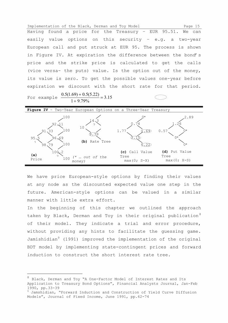
Implementation of the Black, Derman and Toy Model Page 15 Having found a price for the Treasury – EUR 95.51. We can
easily value options on this security – e.g. a two-year
European call and put struck at EUR 95. The process is shown
in Figure IV. At expiration the difference between the bond’s
price and the strike price is calculated to get the calls
(vice versa- the puts) value. Is the option out of the money,
its value is zero. To get the possible values one-year before
expiration we discount with the short rate for that period.
For example 15.3%79.91
)22.5(5.0)69.1(5.0=
++
Figure IV – Two-Year European Options on a Three-Year Treasury
We have price European-style options by finding their values
at any node as the discounted expected value one step in the
future. American-style options can be valued in a similar
manner with little extra effort.
In the beginning of this chapter we outlined the approach
taken by Black, Derman and Toy in their original publication8
of their model. They indicate a trial and error procedure,
without providing any hints to facilitate the guessing game.
Jamishidian9 (1991) improved the implementation of the original
BDT model by implementing state-contingent prices and forward
induction to construct the short interest rate tree.
8 Black, Derman and Toy “A One-Factor Model of Interest Rates and Its Application to Treasury Bond Options”, Financial Analysts Journal, Jan-Feb 1990, pp.33-39 9 Jamshidian, “Forward Induction and Construction of Yield Curve Diffusion Models”, Journal of Fixed Income, June 1991, pp.62-74
95.51
91.33
98.79
92.11
96.69
100.22
100
100
100
100
10
14.32
9.79 1.77
0.74
3.15
0*
1.69
5.22
(c) Call Value Tree max(0; S-X)
0.57
1.26
0*
2.89
0*
0*
(d) Put Value Tree max(0; X-S)
(b) Rate Tree
(a) Price (* … out of the
money)
Implementation of the Black, Derman and Toy Model Page 16 Bjerksund and Stensland 10 developed an alternative to
Jamshidian’s forward induction method which proves to be even
more efficient. With the help of two formulas they provide a
closed form solution to the calibration problem. Given the
initial yield and volatility curves a bond price tree is
modeled that helps to approximate the short interest rate tree.
The idea is to use information from the calculated tree to
adjust input, which is used to generate a new tree by the two
approximation formulas. Avoiding iteration procedures they
assure shorter computation times and accurate results.
4.3. The BDT-Model and Reality
The BDT model offers in comparison to the Ho-Lee model more
flexibility. In the case of constant volatility the expected
yield of the Ho-Lee model moves exactly parallel, but the BDT
model allows more complex changes in the yield-curve shape.
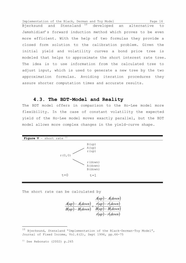
Figure V – short rate 11
The short rate can be calculated by
( ) ( )( ) ( )
( ) ( )( ) ( )( ) ( )( ) ( )downrupr
downBupBdownruprdownAupA
downBupBdownAupA
−−−−
=−−
10 Bjerksund, Stensland “Implementation of the Black-Derman-Toy Model”, Journal of Fixed Income, Vol.6(2), Sept 1996, pp.66-75 11 See Rebonato (2002) p.265
r(0,0)
B(up) A(up) r(up)
r(down) A(down) B(down)
t=0 t=1
Implementation of the Black, Derman and Toy Model Page 17 From the equation above (right side) we can easily derive the
sensitivity of Bond prices of different maturities to changes
in the short rates.12
The sensitivity of the short rates is strongly dependent on
the shape of the yield curve. Upward sloping term structure
tend to produce an elasticity above 1.
It must be stressed that using BDT, which is a one-factor
model, does not mean that the yield curve is forced to move
parallel. The crucial point is that only one source of
uncertainty is allowed to affect the different rates. In
contrast to linearly independent rates, a one factor model
implies that all rates are perfectly correlated. Of course,
rates with different maturity are not perfectly correlated.
One factor models are brutally simplifying real life. So two
(or three) factor models would be a better choice to match the
rates. 13
12 See Rebonato (2002) p.264 13 Francke (2000) p.11-14
Implementation of the Black, Derman and Toy Model Page 18 Mainly three advantages using one factor models rather than
two or three factor models can be mentioned:
1. It is easier to implement
2. It takes much less computer time
3. It is much easier to calibrate
The ease of calibration to caps is one of the advantages in
the case of the BDT model. It is considered by many
practitioners to outperform all other one-factor models.
The BDT model suffers from two important disadvantages14:
• Substantial inability to handle conditions where the
impact of a second factor could be of relevance because
of the one-factor model
• Inability to specify the volatility of yields of
different maturities independently of future volatility
of the short rate
An exact match of the volatilities of yields of different
maturities should not be expected and, even if actually
observed, should be regarded as a little more than fortuitous.
Another disadvantage of the BDT model is that the fundamental
idea of a short rate process, that follows a mean reversion,
does not hold under the following circumstance. If the
continuous time BDT risk neutral short rate process has the
form:
( ) ( ) ( ) ( )[ ]{ } ( ) ( )tdztdttrtfttrd ⋅+⋅−⋅+= σψθ lnln ,
where:
( )tu .. is the median of the short rate distribution at time t
( ) ( )t
tut∂
∂=
lnθ
( )t
tf∂
∂−=
σln,
( ) ( )tut ln=ψ
14 See Rebonato (2002) p.268
Implementation of the Black, Derman and Toy Model Page 19 For constant volatility ( const=σ ), 0, =f , the BDT model does not
display any mean reversion.
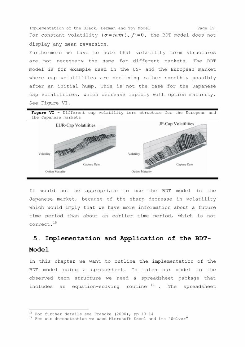
Furthermore we have to note that volatility term structures
are not necessary the same for different markets. The BDT
model is for example used in the US- and the European market
where cap volatilities are declining rather smoothly possibly
after an initial hump. This is not the case for the Japanese
cap volatilities, which decrease rapidly with option maturity.
See Figure VI.
Figure VI - Different cap volatility term structure for the European and the Japanese markets
It would not be appropriate to use the BDT model in the
Japanese market, because of the sharp decrease in volatility
which would imply that we have more information about a future
time period than about an earlier time period, which is not
correct.15
5. Implementation and Application of the BDT-
Model
In this chapter we want to outline the implementation of the
BDT model using a spreadsheet. To match our model to the
observed term structure we need a spreadsheet package that
includes an equation-solving routine 16 . The spreadsheet
15 For further details see Francke (2000), pp.13-14 16 For our demonstration we used Microsoft Excel and its “Solver”
Implementation of the Black, Derman and Toy Model Page 20 equation takes advantage of the forward equation and is an
appropriate method when the number of periods is not large.
A simple way 17 of writing our model is to assume that the
values in the short rate (rks) lattice are of the form
sbkks
kear =
We index the nodes of a short rate lattice according to the
format (k,s), where k is the time (k=0,1,…,n) and s is the
state (s=0,1,…,k). Here ak is a measure of the aggregate drift,
bk represents the volatility of the logarithm of the short rate
from time k-1 to k. Many practitioners choose to fit the rate
structure only 18 , holding the future short rate volatility
constant19. So in the simplest version of the model, the values
of bk are all equal to one value b. The ak’s are then assigned
so that the implied term structure matches the observed term
structure.
(Step 1) We get the data of a yield curve and paste it into
Excel. 20 To match it to our BDT model, we have to make
assumptions concerning volatility. For our case we suppose to
have measured the volatility to be 0.01 per year, which means
that the short rate is likely to fluctuate about one
percentage point during a year. (Inputs are shown with grey
background in Figure VII a)
(Step 2) We introduce a row for the parameters ak. These
parameters are considered variable by the program. Based on
these parameters the short rate lattice is constructed. We can
enter some values close to the observed spot rate, so we can
neatly see the development of the lattices. What we have done
so far is shown in Figure VII a.
17 See Luenberger (1998), p.400 18 For a justification of this see Clewlow and Strickland (1998) Section 7.7. (pp.222-223) 19 The convergent continuous time limit as shown on page 8 therefore reduces to the following equation : d ln r = θ(t) dt + σ dz . This process can be seen as a lognormal version of the Ho and Lee model. 20 In our case we obtained the spot rate curve from the ÖKB website (http://www.profitweb.at/apps/ yieldcourse/index.jsp).
Implementation of the Black, Derman and Toy Model Page 21
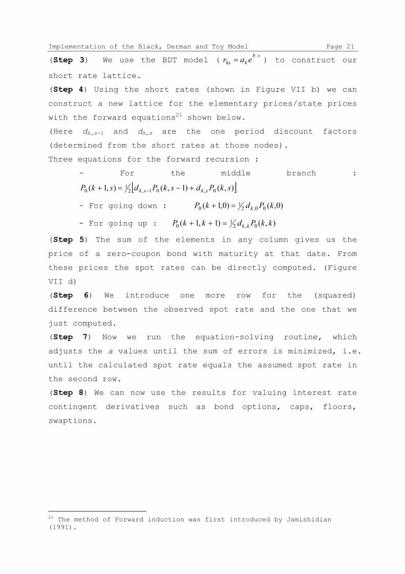
(Step 3) We use the BDT model (sb
kks ear = ) to construct our
short rate lattice.
(Step 4) Using the short rates (shown in Figure VII b) we can
construct a new lattice for the elementary prices/state prices
with the forward equations21 shown below.
(Here dk,s-1 and dk,s are the one period discount factors
(determined from the short rates at those nodes).
Three equations for the forward recursion :
- For the middle branch :
[ ]),()1,(),1( 0,01,21
0 skPdskPdskP sksk +−=+ −
- For going down : )0,()0,1( 00,21
0 kPdkP k=+
- For going up : ),()1,1( 0,21
0 kkPdkkP kk=++
(Step 5) The sum of the elements in any column gives us the
price of a zero-coupon bond with maturity at that date. From
these prices the spot rates can be directly computed. (Figure
VII d)
(Step 6) We introduce one more row for the (squared)
difference between the observed spot rate and the one that we
just computed.
(Step 7) Now we run the equation-solving routine, which
adjusts the a values until the sum of errors is minimized, i.e.
until the calculated spot rate equals the assumed spot rate in
the second row.
(Step 8) We can now use the results for valuing interest rate
contingent derivatives such as bond options, caps, floors,
swaptions.
21 The method of Forward induction was first introduced by Jamishidian (1991).
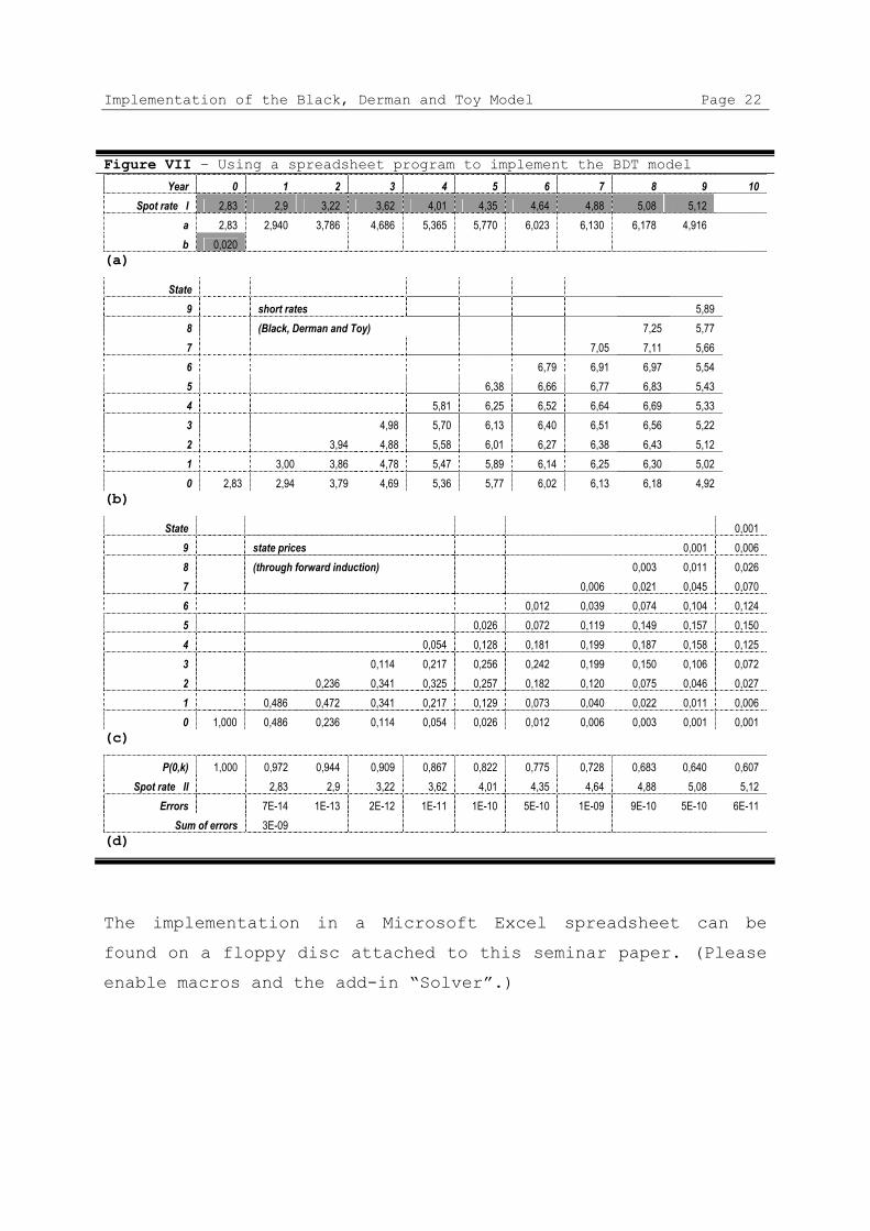
Implementation of the Black, Derman and Toy Model Page 22 Figure VII – Using a spreadsheet program to implement the BDT model
Year 0 1 2 3 4 5 6 7 8 9 10 Spot rate I 2,83 2,9 3,22 3,62 4,01 4,35 4,64 4,88 5,08 5,12
a 2,83 2,940 3,786 4,686 5,365 5,770 6,023 6,130 6,178 4,916 b 0,020
(a)
State 9 short rates 5,89 8 (Black, Derman and Toy) 7,25 5,77 7 7,05 7,11 5,66 6 6,79 6,91 6,97 5,54 5 6,38 6,66 6,77 6,83 5,43 4 5,81 6,25 6,52 6,64 6,69 5,33 3 4,98 5,70 6,13 6,40 6,51 6,56 5,22 2 3,94 4,88 5,58 6,01 6,27 6,38 6,43 5,12 1 3,00 3,86 4,78 5,47 5,89 6,14 6,25 6,30 5,02 0 2,83 2,94 3,79 4,69 5,36 5,77 6,02 6,13 6,18 4,92
(b)
State 0,001 9 state prices 0,001 0,006 8 (through forward induction) 0,003 0,011 0,026 7 0,006 0,021 0,045 0,070 6 0,012 0,039 0,074 0,104 0,124 5 0,026 0,072 0,119 0,149 0,157 0,150 4 0,054 0,128 0,181 0,199 0,187 0,158 0,125 3 0,114 0,217 0,256 0,242 0,199 0,150 0,106 0,072 2 0,236 0,341 0,325 0,257 0,182 0,120 0,075 0,046 0,027 1 0,486 0,472 0,341 0,217 0,129 0,073 0,040 0,022 0,011 0,006 0 1,000 0,486 0,236 0,114 0,054 0,026 0,012 0,006 0,003 0,001 0,001
(c)
P(0,k) 1,000 0,972 0,944 0,909 0,867 0,822 0,775 0,728 0,683 0,640 0,607 Spot rate II 2,83 2,9 3,22 3,62 4,01 4,35 4,64 4,88 5,08 5,12
Errors 7E-14 1E-13 2E-12 1E-11 1E-10 5E-10 1E-09 9E-10 5E-10 6E-11 Sum of errors 3E-09
(d)
The implementation in a Microsoft Excel spreadsheet can be
found on a floppy disc attached to this seminar paper. (Please
enable macros and the add-in “Solver”.)
Implementation of the Black, Derman and Toy Model Page 23
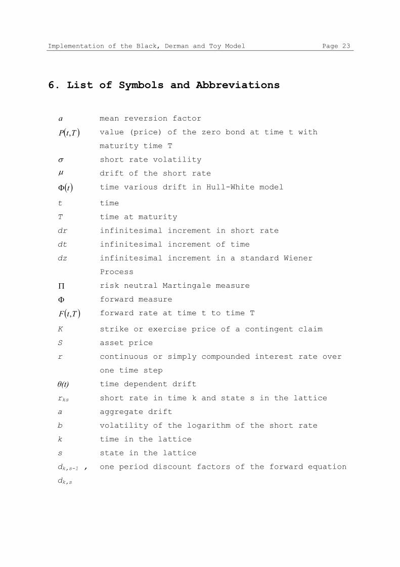
6. List of Symbols and Abbreviations
a mean reversion factor
( )TtP , value (price) of the zero bond at time t with
maturity time T
σ short rate volatility
µ drift of the short rate
( )tΦ time various drift in Hull-White model
t time
T time at maturity
dr infinitesimal increment in short rate
dt infinitesimal increment of time
dz infinitesimal increment in a standard Wiener
Process
Π risk neutral Martingale measure
Φ forward measure
( )TtF , forward rate at time t to time T
K strike or exercise price of a contingent claim
S asset price
r continuous or simply compounded interest rate over
one time step
θ(t) time dependent drift
rks short rate in time k and state s in the lattice
a aggregate drift
b volatility of the logarithm of the short rate
k time in the lattice
s state in the lattice
dk,s-1 ,
dk,s
one period discount factors of the forward equation
Implementation of the Black, Derman and Toy Model Page 24
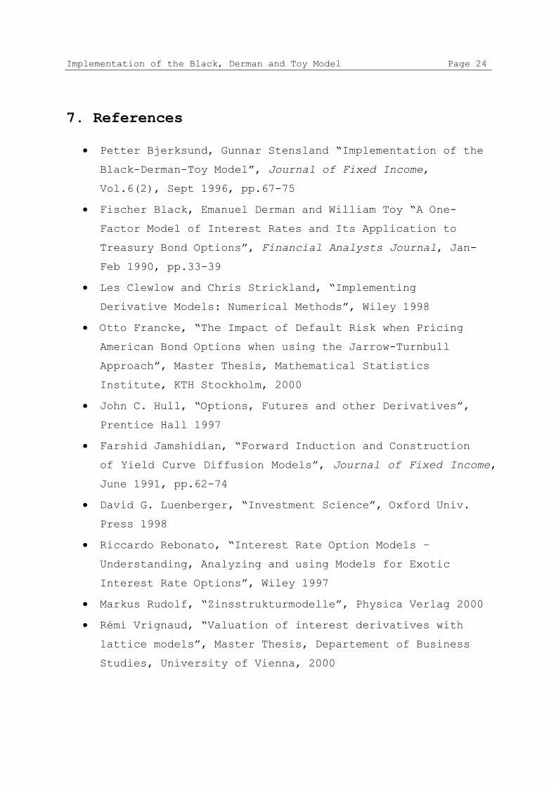
7. References
• Petter Bjerksund, Gunnar Stensland “Implementation of the
Black-Derman-Toy Model”, Journal of Fixed Income,
Vol.6(2), Sept 1996, pp.67-75
• Fischer Black, Emanuel Derman and William Toy “A One-
Factor Model of Interest Rates and Its Application to
Treasury Bond Options”, Financial Analysts Journal, Jan-
Feb 1990, pp.33-39
• Les Clewlow and Chris Strickland, “Implementing
Derivative Models: Numerical Methods”, Wiley 1998
• Otto Francke, “The Impact of Default Risk when Pricing
American Bond Options when using the Jarrow-Turnbull
Approach”, Master Thesis, Mathematical Statistics
Institute, KTH Stockholm, 2000
• John C. Hull, “Options, Futures and other Derivatives”,
Prentice Hall 1997
• Farshid Jamshidian, “Forward Induction and Construction
of Yield Curve Diffusion Models”, Journal of Fixed Income,
June 1991, pp.62-74
• David G. Luenberger, “Investment Science”, Oxford Univ.
Press 1998
• Riccardo Rebonato, “Interest Rate Option Models –
Understanding, Analyzing and using Models for Exotic
Interest Rate Options”, Wiley 1997
• Markus Rudolf, “Zinsstrukturmodelle”, Physica Verlag 2000
• Rémi Vrignaud, “Valuation of interest derivatives with
lattice models”, Master Thesis, Departement of Business
Studies, University of Vienna, 2000
Implementation of the Black, Derman and Toy Model Page 25
8. Suggestions for further reading
• T.G., Bali, Karagozoglu “Implementation of the BDT-Model
with Different Volatility Estimators”, Journal of Fixed
Income, March 1999, pp.24-34
• Fischer Black, Piotr Karasinsky , “Bond and Option
Pricing when Short Rates are Lognormal”, Financial
Analysts Journal, July-August 1991, pp.52-59
• John Hull, Alan White, “New Ways with the Yield Curve”,
Risk, October 1990a
• John Hull, Alan White, “One Factor Interest-Rate Models
and the Valuation of Interest-Rate Derivative Securities”,
Journal of Financial and Quantitative Analysis, Vol. 28,
June 1993, pp.235-254
• John Hull, Alan White, “Pricing Interest-Rate Derivative
Securities”, Review of Financial Studies, Vol. 4, 1990b,
pp.573-591
• R. Jarrow and S. Turnbull “Pricing Derivatives on
Financial Securities subject to Credit Risk”. The Journal
of Finance, March 1995, pp. 53-85
• R. Jarrow, D. Lando and Turnbull, “A Markov Model for the
Term Structure of Credit Risk Spreads”. The review of
financial studies, 1997 Vol. 10, No.2.


