* Corresponding author: w.zuo@miami.edu

Huang, S., Zuo, W., Sohn, M. “Improved Cooling Tower Control of Legacy Chiller Plants by

Optimizing the Condenser Water Set Point,” Building and Environment, 111, pp. 33-46, 2017.

Improved Cooling Tower Control of Legacy Chiller Plants by

Optimizing the Condenser Water Set Point

Sen Huang a+, Wangda Zuo a,*, Michael D. Sohn b

a Department of Civil, Architectural and Environmental Engineering, University of Miami,

1251 Memorial Drive, Coral Gables, FL 33146, U.S.A. b Energy Analysis and Environmental Impacts Division, Lawrence Berkeley National

Laboratory, 1 Cyclotron Road, Berkeley, CA 94720, U.S.A. + Current Address: Electricity Infrastructure and Buildings Division, Pacific Northwest National

Laboratory, 902 Battelle Boulevard, WA 99354, U.S.A.

Abstract:

Achieving the optimal control of cooling towers is critical to the energy-efficient operation of current or

legacy chiller plants. Although many promising control methods have been proposed, limitations in their

applications exist for legacy chiller plants. For example, some methods require the change of the plant’s

overall control structure, which can be difficult to legacy chiller plants; some methods are too complicated

and computationally intensive to implement in old building control systems. To address the above issues,

we develop an operational support system. This system employs a model predictive control scheme to

optimize the condenser water set point and can be applied in chiller plants without changes in the control

structure. To further facilitate the implementation, we propose to increase the optimization accuracy by

selecting a better starting point. The results from a case study with a real legacy chiller plant in Washington

D.C. show that the proposed operational support system can achieve up to around 9.67% annual energy

consumption savings for chillers and cooling towers. The results also show the proposed starting point

selection method can achieve a better accuracy and a faster computational speed than commonly used

methods. In addition, we find that we can select a lower optimization frequency for the studied case since

the impact of the optimization frequency on the energy savings is not significant while a lower optimization

frequency does reduce the computational demand to a great extent.

2

Keywords: Model Predictive Control; Condenser Water Set Point; Optimization Starting Point;

Optimization Frequency; Modelica

Nomenclature

𝑡 Time

𝐸|𝑡0

𝑡0+Δ𝑡 Energy consumption during the optimization period [𝑡0, 𝑡0 + ∆𝑡)

𝑃 Power

𝑇 Temperature

�̇� Cooling load

𝑆 State vector

𝑃𝐿𝑅 Part load ratio

𝐶𝑂𝑃 Coefficient of performance

𝜀 Effectiveness

𝑐 Constant coefficient

𝑦 Cooling tower fan speed ratio

Superscript

𝑃 Predicted

∗ With error

Subscript

𝑐𝑤 Condenser water

𝑐ℎ𝑤 Chilled water

𝑠𝑒𝑡 Set point

𝑤𝑏 Outdoor wet bulb temperature

𝐿 Low limit

𝐻 High limit

𝑙𝑜𝑤 The lowest possible value

ℎ𝑖𝑔 The highest possible value

𝑡𝑤 Cooling tower

3

𝑐ℎ Chiller

𝑒𝑛𝑡 Entering the chiller

𝑙𝑒𝑎 Leaving the chiller

𝑠𝑡𝑎 Starting point

𝑎𝑝𝑝 Approach

𝑛𝑜𝑚 Nominal

𝑒𝑣𝑎 Evaporator

𝑐𝑜𝑛 Condenser

𝑠𝑡𝑎𝑒𝑟𝑟 Static error

4

* Corresponding author: w.zuo@miami.edu

1. Introduction

Chiller plants are widely used to provide cooling to buildings [1]. As a result, about 5.17×1011 MJ annual

energy consumption in the commercial buildings is attributed to chillers alone, which are the key

components of chiller plants [1]. Including other components, such as cooling towers and pumps, the total

energy consumption by chiller plants is even higher. Thus, it is necessary to enhance the energy efficiency

of chiller plants.

Depending on how chillers reject the waste heat, chiller plants can be categorized as water-cooled and air-

cooled. Water-cooled chiller plants with cooling towers are commonly used for large buildings. A typical

water-cooled chiller plant consists of two water loops: a chilled water loop and a condenser water loop. The

chilled water loop transfers the cooling energy generated by the chiller to the demand side; the condenser

water loop rejects the waste heat from the chiller to the ambient environment through the water evaporation

occurs in cooling towers [2].

Water-cooled chiller plants are typically controlled by a two-level control structure. The low-level control

(local controller) is enabled by a feedback control system. For instance, the temperature of the condenser

water leaving the cooling towers is typically controlled by adjusting the speed of the cooling tower fans to

meet a predefined set point, which is referred as condenser water set point. The upper-level control

(supervisor controller) is used to specify set points for the local controller and other time-dependent modes

of operation [2]. Conventionally, set points are fixed at the nominal values.

One commonly used approach to improve energy efficiency of chiller plants is to optimize the control of

the cooling towers: one can reduce chiller energy consumption by increasing cooling tower fan speeds so

that the temperature of the condenser water entering the chillers is reduced. However, higher fan speeds

mean that cooling towers will use more energy. Thus, the goal is to minimize the total energy consumption

of cooling towers and chillers by adjusting the fan speeds of cooling towers.

Due to the nonlinear nature of chiller plant energy use, identifying the optimal cooling tower fan speed is

challenging. For example, the energy performance curves of chillers and cooling towers are usually

nonlinear and sometimes non-convex, which means the commonly used system analysis tools, such as

linear optimization methods, may not be suitable for this problem. In addition, according to the ASHRAE

Handbook [2], the optimal fan speeds of cooling towers may be affected by both the cooling load and

weather conditions. Therefore, finding optimal cooling tower fan speed is also a multiple-input problem.

6

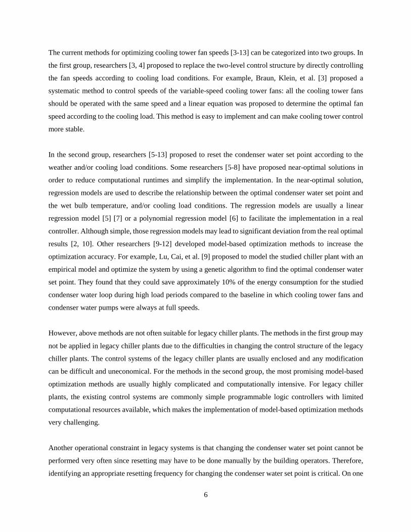
The current methods for optimizing cooling tower fan speeds [3-13] can be categorized into two groups. In

the first group, researchers [3, 4] proposed to replace the two-level control structure by directly controlling

the fan speeds according to cooling load conditions. For example, Braun, Klein, et al. [3] proposed a

systematic method to control speeds of the variable-speed cooling tower fans: all the cooling tower fans

should be operated with the same speed and a linear equation was proposed to determine the optimal fan

speed according to the cooling load. This method is easy to implement and can make cooling tower control

more stable.

In the second group, researchers [5-13] proposed to reset the condenser water set point according to the

weather and/or cooling load conditions. Some researchers [5-8] have proposed near-optimal solutions in

order to reduce computational runtimes and simplify the implementation. In the near-optimal solution,

regression models are used to describe the relationship between the optimal condenser water set point and

the wet bulb temperature, and/or cooling load conditions. The regression models are usually a linear

regression model [5] [7] or a polynomial regression model [6] to facilitate the implementation in a real

controller. Although simple, those regression models may lead to significant deviation from the real optimal

results [2, 10]. Other researchers [9-12] developed model-based optimization methods to increase the

optimization accuracy. For example, Lu, Cai, et al. [9] proposed to model the studied chiller plant with an

empirical model and optimize the system by using a genetic algorithm to find the optimal condenser water

set point. They found that they could save approximately 10% of the energy consumption for the studied

condenser water loop during high load periods compared to the baseline in which cooling tower fans and

condenser water pumps were always at full speeds.

However, above methods are not often suitable for legacy chiller plants. The methods in the first group may

not be applied in legacy chiller plants due to the difficulties in changing the control structure of the legacy

chiller plants. The control systems of the legacy chiller plants are usually enclosed and any modification

can be difficult and uneconomical. For the methods in the second group, the most promising model-based

optimization methods are usually highly complicated and computationally intensive. For legacy chiller

plants, the existing control systems are commonly simple programmable logic controllers with limited

computational resources available, which makes the implementation of model-based optimization methods

very challenging.

Another operational constraint in legacy systems is that changing the condenser water set point cannot be

performed very often since resetting may have to be done manually by the building operators. Therefore,

identifying an appropriate resetting frequency for changing the condenser water set point is critical. On one

7

side, a low resetting frequency can reduce efforts by the building operators. On the other side, a low

frequency may reduce the energy savings due to the failure in capitalizing on the system dynamics; in

addition, a lower optimization frequency leads to a longer prediction horizon for model inputs. The

prediction accuracy will be likely decreased with a longer prediction horizon [14], which means more

uncertainties will be introduced into the optimization. Thus, it is important to quantitatively evaluate the

impact of the optimization frequency on the energy consumption by chiller plants.

This study attempts to develop an operational support system to optimize cooling tower operation for legacy

chiller plants. Our system uses the predicted cooling load and wet bulb temperature as inputs for a model

predictive scheme to search the optimal condenser water set points for a future period. The operators can

then manually change the set points in the chiller control system, which alleviates the difficulty in the

implementation for legacy building systems as it does not require the deployment of the algorithms in

existing legacy controllers. To improve the optimization accuracy and increase the optimization speed, we

also proposed an approach temperature based method for the selection of optimal search starting point. The

proposed method was then assessed using a case study on a legacy chiller plant located in Washington D.C.

In this case study, the energy saving is estimated based on offline simulations. To quantify the impact of

set points changing frequency on the energy savings, we also evaluated the energy savings with different

optimization frequencies in the case study.

Compared to the existing literature, this study makes the following contributions: first, we proposed an

operational support system to optimize the cooling tower operation for legacy chiller plants, which is easier

to implement than existing methods. Second, an approach temperature based method for selecting the

starting point was developed to improve the accuracy and increase the speed of the model-based condenser

water set point optimization. The approach temperature based method demonstrated a better performance

compared to three commonly used methods. Third, we presented a systematic evaluation for the impact of

the optimization frequency on the energy savings by the condenser water set point optimization. The

evaluation can help operators determine the optimal resetting frequency.

2. Model Predictive Control for Optimizing the Condenser Water Set Point

2.1 Optimization Problem Definition

For the condenser water set point optimization, we consider a water-cooled chiller plant with multiple

chillers and multiple cooling towers. The primary chilled water pumps and condenser water pumps are

constant speed pumps. For each cooling tower, there is a variable speed fan controlled by one condenser

water set point. We assume that all the cooling towers are controlled by the same condenser water set point

8

and there is no other independent variable in the optimization. Since the change of the condenser water set

point doesn’t affect the operation of pumps, the optimization problem can be defined as

argmin

𝑇𝑐𝑤,𝑠𝑒𝑡(𝑡0)(𝐸𝑡𝑜𝑡|𝑡0

𝑡0+Δ𝑡) = min (∫ (𝑃𝑐ℎ(𝑡) +

𝑡0+∆𝑡

𝑡0

𝑃𝑡𝑤(𝑡))𝑑𝑡)

for 𝑡 ∈ [𝑡0, 𝑡0 + ∆𝑡)

(1)

𝑃𝑐ℎ(𝑡) = 𝑓(𝑇𝑐𝑤,𝑒𝑛𝑡(𝑡), �̇�𝑃(𝑡), 𝑆𝑐ℎ(𝑡)) (2)

𝑃𝑡𝑤(𝑡) = 𝑓(𝑇𝑤𝑏𝑃 (𝑡), 𝑇𝑐𝑤,𝑠𝑒𝑡(𝑡0), 𝑇𝑐𝑤,𝑙𝑒𝑎(𝑡), 𝑆𝑡𝑤(𝑡)) (3)

s.t. 𝑇𝑐𝑤,𝑠𝑒𝑡,𝐿 ≤ 𝑇𝑐𝑤,𝑠𝑒𝑡(𝑡0) ≤ 𝑇𝑐𝑤,𝑠𝑒𝑡,𝐻, (4)

𝑇𝑐𝑤,𝑒𝑛𝑡(𝑡) = 𝑓(𝑇𝑤𝑏𝑃 (𝑡), 𝑇𝑐𝑤,𝑠𝑒𝑡(𝑡0), 𝑇𝑐𝑤,𝑙𝑒𝑎(𝑡), 𝑆𝑡𝑤), (5)

𝑇𝑐𝑤,𝑙𝑒𝑎(𝑡) = 𝑓(�̇�𝑃(𝑡), 𝑃𝑐ℎ(𝑡), 𝑇𝑐𝑤,𝑒𝑛𝑡(𝑡), 𝑆𝑐ℎ), (6)

where 𝐸𝑡𝑜𝑡|𝑡0

𝑡0+Δ𝑡 is the total energy consumption of the chillers and cooling towers during the optimization

period [𝑡0, 𝑡0 + ∆𝑡), 𝑃𝑐ℎ is the power of the chillers while 𝑃𝑡𝑤 is the power of the cooling towers, 𝑇𝑐𝑤,𝑠𝑒𝑡

is the condenser water set point, �̇�𝑃 is the predicted cooling load over [𝑡0, 𝑡0 + ∆𝑡), 𝑇𝑤𝑏𝑃 is the predicted

wet bulb temperature over [𝑡0, 𝑡0 + ∆𝑡), 𝑇𝑐𝑤,𝑒𝑛𝑡 and 𝑇𝑐𝑤,𝑙𝑒𝑎 are the temperature of the condenser water

entering and leaving the chillers, respectively. 𝑆𝑐ℎ and 𝑆𝑡𝑤 are the state vectors of the chillers and the

cooling towers (e.g. equipment operating status, water temperature in chiller condenser and evaporator),

respectively. 𝑇𝑐𝑤,𝑠𝑒𝑡,𝐿 and 𝑇𝑐𝑤,𝑠𝑒𝑡,𝐻 are the low and high limits of the condenser water set point during

[𝑡0, 𝑡0 + ∆𝑡). Using the evaporative cooling, the cooling tower cannot cool the condenser water to a

temperature lower than the outdoor web bulb temperature, 𝑇𝑤𝑏. Thus, the actual 𝑇𝑐𝑤,𝑠𝑒𝑡,𝐿 can be determined

by

𝑇𝑐𝑤,𝑠𝑒𝑡,𝐿 = 𝑚𝑖𝑛𝑖𝑚𝑢𝑚{𝑇𝑖 ∈ {𝑇1, … , 𝑇𝑛} | 𝑇𝑖 ≥ 𝑇𝑤𝑏,𝐿𝑃 }, (7)

where {𝑇1, … , 𝑇𝑛} is the set of all the possible values for the condenser water set point, 𝑇𝑤𝑏,𝐿𝑃 is the lowest

𝑇𝑤𝑏𝑃 during [𝑡0, 𝑡0 + ∆𝑡). The 𝑇𝑐𝑤,𝑠𝑒𝑡,𝐻 is set as

𝑇𝑐𝑤,𝑠𝑒𝑡,𝐻 = 𝑚𝑎𝑥𝑖𝑚𝑢𝑚 {𝑇1, … , 𝑇𝑛} . (8)

In addition, �̇�𝑃 can be estimated using the load prediction model shown in [15] and 𝑇𝑤𝑏𝑃 (𝑡) can be obtained

from the weather forecast service.

2.2 Optimization Framework for Chiller Plants

To implement the optimization described in the section 2.1, we developed a framework for the chiller plant

controls optimization. The core of the framework is a system model of the studied chiller plant and an

optimization engine. The plant model can be re-initialized during the runtime for continuous optimization.

9

In addition, Python scripts are developed to automate the pre-processing, optimization and post-processing

processes.

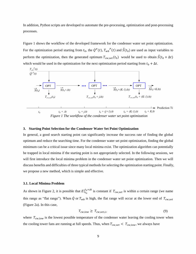
Figure 1 shows the workflow of the developed framework for the condenser water set point optimization.

For the optimization period starting from 𝑡0, the �̇�𝑃(𝑡), 𝑇𝑤𝑏𝑃(𝑡) and 𝑆(𝑡0) are used as input variables to

perform the optimization, then the generated optimum 𝑇𝑐𝑤,𝑠𝑒𝑡(𝑡0) would be used to obtain 𝑆(𝑡0 + ∆𝑡)

which would be used in the optimization for the next optimization period starting from 𝑡0 + ∆𝑡.

Figure 1 The workflow of the condenser water set point optimization

3. Starting Point Selection for the Condenser Water Set Point Optimization

In general, a good search starting point can significantly increase the success rate of finding the global

optimum and reduce the searching time. For the condenser water set point optimization, finding the global

minimum can be a critical issue since many local minima exist. The optimization algorithm can potentially

be trapped in local minima if the starting point is not appropriately selected. In the following sessions, we

will first introduce the local minima problem in the condenser water set point optimization. Then we will

discuss benefits and difficulties of three typical methods for selecting the optimization starting point. Finally,

we propose a new method, which is simple and effective.

3.1. Local Minima Problem

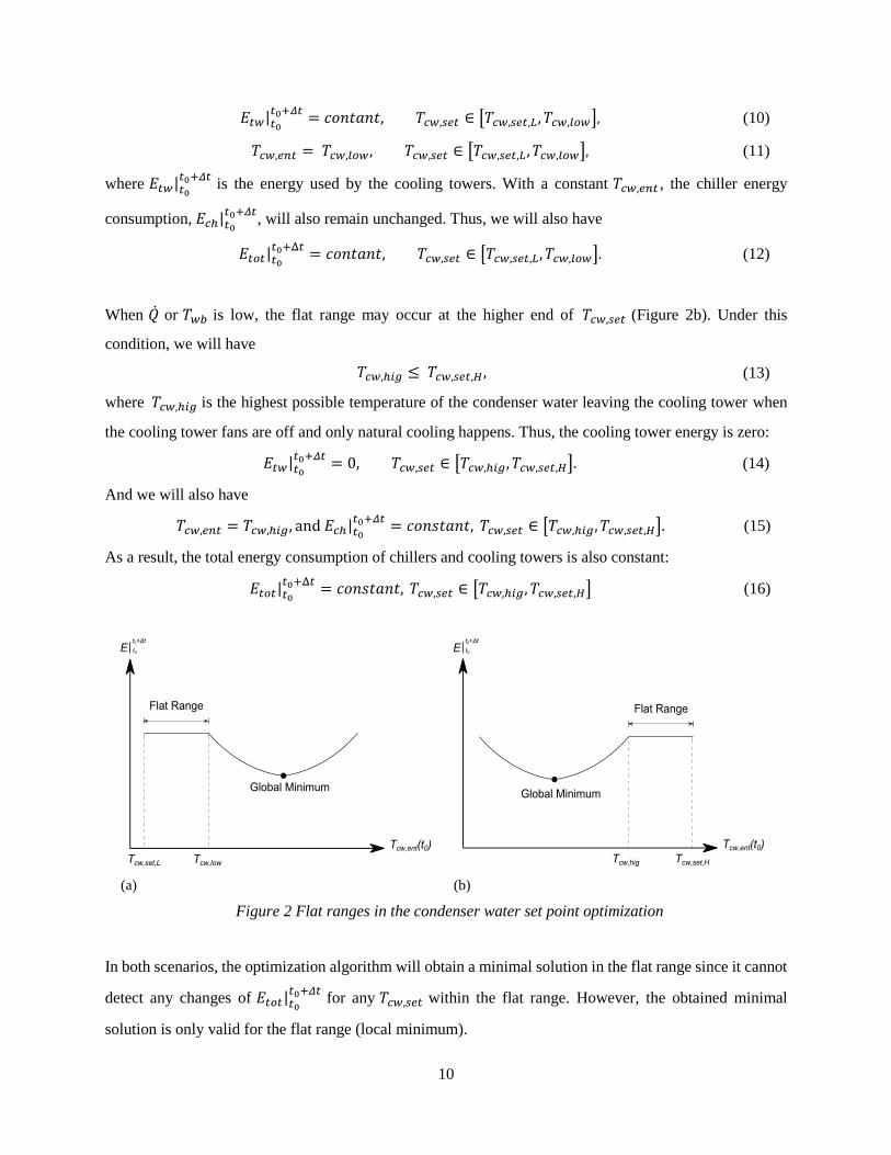
As shown in Figure 2, it is possible that 𝐸|𝑡0

𝑡0+𝛥𝑡 is constant if 𝑇𝑐𝑤,𝑠𝑒𝑡 is within a certain range (we name

this range as “flat range”). When �̇� or 𝑇𝑤𝑏 is high, the flat range will occur at the lower end of 𝑇𝑐𝑤,𝑠𝑒𝑡

(Figure 2a). In this case,

𝑇𝑐𝑤,𝑙𝑜𝑤 ≥ 𝑇𝑐𝑤,𝑠𝑒𝑡,𝐿 , (9)

where 𝑇𝑐𝑤,𝑙𝑜𝑤 is the lowest possible temperature of the condenser water leaving the cooling tower when

the cooling tower fans are running at full speeds. Thus, when 𝑇𝑐𝑤,𝑠𝑒𝑡 < 𝑇𝑐𝑤,𝑙𝑜𝑤, we always have

10

𝐸𝑡𝑤|𝑡0

𝑡0+𝛥𝑡= 𝑐𝑜𝑛𝑡𝑎𝑛𝑡, 𝑇𝑐𝑤,𝑠𝑒𝑡 ∈ [𝑇𝑐𝑤,𝑠𝑒𝑡,𝐿, 𝑇𝑐𝑤,𝑙𝑜𝑤], (10)

𝑇𝑐𝑤,𝑒𝑛𝑡 = 𝑇𝑐𝑤,𝑙𝑜𝑤, 𝑇𝑐𝑤,𝑠𝑒𝑡 ∈ [𝑇𝑐𝑤,𝑠𝑒𝑡,𝐿 , 𝑇𝑐𝑤,𝑙𝑜𝑤], (11)

where 𝐸𝑡𝑤|𝑡0

𝑡0+𝛥𝑡 is the energy used by the cooling towers. With a constant 𝑇𝑐𝑤,𝑒𝑛𝑡 , the chiller energy

consumption, 𝐸𝑐ℎ|𝑡0

𝑡0+𝛥𝑡, will also remain unchanged. Thus, we will also have

𝐸𝑡𝑜𝑡|𝑡0

𝑡0+Δ𝑡= 𝑐𝑜𝑛𝑡𝑎𝑛𝑡, 𝑇𝑐𝑤,𝑠𝑒𝑡 ∈ [𝑇𝑐𝑤,𝑠𝑒𝑡,𝐿 , 𝑇𝑐𝑤,𝑙𝑜𝑤]. (12)

When �̇� or 𝑇𝑤𝑏 is low, the flat range may occur at the higher end of 𝑇𝑐𝑤,𝑠𝑒𝑡 (Figure 2b). Under this

condition, we will have

𝑇𝑐𝑤,ℎ𝑖𝑔 ≤ 𝑇𝑐𝑤,𝑠𝑒𝑡,𝐻 , (13)

where 𝑇𝑐𝑤,ℎ𝑖𝑔 is the highest possible temperature of the condenser water leaving the cooling tower when

the cooling tower fans are off and only natural cooling happens. Thus, the cooling tower energy is zero:

𝐸𝑡𝑤|𝑡0

𝑡0+𝛥𝑡= 0, 𝑇𝑐𝑤,𝑠𝑒𝑡 ∈ [𝑇𝑐𝑤,ℎ𝑖𝑔, 𝑇𝑐𝑤,𝑠𝑒𝑡,𝐻]. (14)

And we will also have

𝑇𝑐𝑤,𝑒𝑛𝑡 = 𝑇𝑐𝑤,ℎ𝑖𝑔, and 𝐸𝑐ℎ|𝑡0

𝑡0+𝛥𝑡= 𝑐𝑜𝑛𝑠𝑡𝑎𝑛𝑡, 𝑇𝑐𝑤,𝑠𝑒𝑡 ∈ [𝑇𝑐𝑤,ℎ𝑖𝑔, 𝑇𝑐𝑤,𝑠𝑒𝑡,𝐻]. (15)

As a result, the total energy consumption of chillers and cooling towers is also constant:

𝐸𝑡𝑜𝑡|𝑡0

𝑡0+Δ𝑡= 𝑐𝑜𝑛𝑠𝑡𝑎𝑛𝑡, 𝑇𝑐𝑤,𝑠𝑒𝑡 ∈ [𝑇𝑐𝑤,ℎ𝑖𝑔, 𝑇𝑐𝑤,𝑠𝑒𝑡,𝐻] (16)

(a)

(b)

Figure 2 Flat ranges in the condenser water set point optimization

In both scenarios, the optimization algorithm will obtain a minimal solution in the flat range since it cannot

detect any changes of 𝐸𝑡𝑜𝑡|𝑡0

𝑡0+𝛥𝑡 for any 𝑇𝑐𝑤,𝑠𝑒𝑡 within the flat range. However, the obtained minimal

solution is only valid for the flat range (local minimum).

11

3.2. Current Methods for Selecting Starting Point

To mitigate the local minima problem in the condenser water set point optimization, it is critical to start the

search outside the flat range. Unfortunately, generic starting point selection methods, such as the middle

point method, the multiple starting point method, and the previous value method may not be well-suited for

avoiding the flat range problem.

The middle point method uses the middle point between the low bound and high bound of the independent

variable as the starting point. Because it is the simplest method to reduce the distance of the starting point

and the global minimum, the middle point method is widely used in optimization problems when only one

global minimum is believed to exist [16, 17]. However, for the optimization problem with multiple local

minima, the middle point method may lead to a local minimum if the local minimum is near the middle

point.

As an improvement of middle point method, a multiple starting point method was proposed [18]. In this

method, multiple starting points are generated randomly from a uniform distribution between the low and

high bounds for the independent variable to increase the possibility that starting points are close to the

global minimum. However, it still does not guarantee the global minimum and may increase the searching

time with multiple starting points [19].

Alternatively, the previous value method [20] uses the optimal value resulted from the previous search as

the starting points of the present search. The previous value method is based on the assumption that the

optimal results for two adjacent optimization periods are likely close if the system states and inputs are

similar. However, it may not work properly if the system states and inputs of two optimization periods are

significantly different.

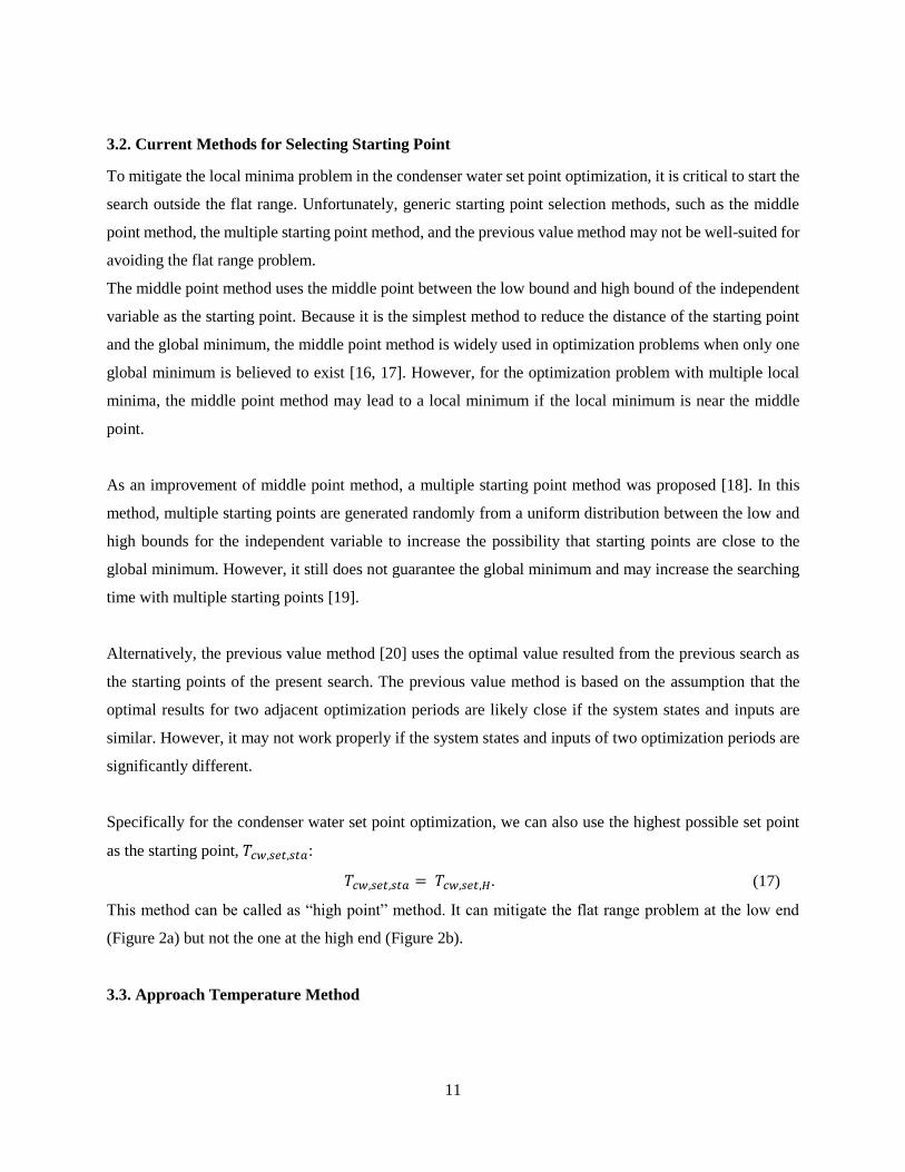
Specifically for the condenser water set point optimization, we can also use the highest possible set point

as the starting point, 𝑇𝑐𝑤,𝑠𝑒𝑡,𝑠𝑡𝑎:

𝑇𝑐𝑤,𝑠𝑒𝑡,𝑠𝑡𝑎 = 𝑇𝑐𝑤,𝑠𝑒𝑡,𝐻. (17)

This method can be called as “high point” method. It can mitigate the flat range problem at the low end

(Figure 2a) but not the one at the high end (Figure 2b).

3.3. Approach Temperature Method

12

To address the limitation of the current starting point selection methods for the condenser water set point

optimization, we propose an approach temperature based method by considering the physics of the chiller

plant. To avoid the flat range, 𝑇𝑐𝑤,𝑠𝑒𝑡,𝑠𝑡𝑎 should satisfy

𝑇𝑐𝑤,𝑠𝑒𝑡,𝑠𝑡𝑎 ∈ [𝑇𝑐𝑤,𝑙𝑜𝑤, 𝑇𝑐𝑤,ℎ𝑖𝑔]. (18)

The challenge is how to predict 𝑇𝑐𝑤,𝑙𝑜𝑤 and 𝑇𝑐𝑤,ℎ𝑖𝑔. Although some sophisticated cooling tower

performance models [21, 22] can be used to predict 𝑇𝑐𝑤,𝑙𝑜𝑤 and 𝑇𝑐𝑤,ℎ𝑖𝑔, they are too complicated for the

starting point selection. In this study, we propose to estimate the 𝑇𝑐𝑤,𝑙𝑜𝑤 based on the nominal approach

temperature Δ𝑇𝑎𝑝𝑝,𝑛𝑜𝑚, which is the difference between the temperature of condenser water leaving the

cooling tower and the wet bulb temperature at the nominal condition. The predicted 𝑇𝑐𝑤,𝑙𝑜𝑤 will be:

𝑇𝑐𝑤,𝑙𝑜𝑤𝑃 = {

𝑇𝑐𝑤,𝑠𝑒𝑡,𝐿 𝑇𝑤𝑏 < 𝑇𝑐𝑤,𝑠𝑒𝑡,𝐿 − Δ𝑇𝑎𝑝𝑝,𝑛𝑜𝑚

𝑇𝑐𝑤,𝑠𝑒𝑡,𝐻 𝑇𝑤𝑏 > 𝑇𝑐𝑤,𝑠𝑒𝑡,𝐻 − Δ𝑇𝑎𝑝𝑝,𝑛𝑜𝑚

𝑟𝑜𝑢𝑛𝑑 (𝑇𝑤𝑏 + Δ𝑇𝑎𝑝𝑝,𝑛𝑜𝑚) 𝑂𝑡ℎ𝑒𝑟𝑠 , (19)

where 𝑟𝑜𝑢𝑛𝑑() is the function shown as follows:

𝑟𝑜𝑢𝑛𝑑(𝑇) = 𝑚𝑎𝑥 {𝑇𝑖 ∈ {𝑇1, … , 𝑇𝑛} | 𝑇𝑖 ≤ 𝑇)}, (20)

where {𝑇1, … , 𝑇𝑛} is the set of all the possible values for 𝑇𝑐𝑤,𝑠𝑒𝑡 defined in equation (7). We then set:

𝑇𝑐𝑤,𝑠𝑒𝑡,𝑠𝑡𝑎 = 𝑇𝑐𝑤,𝑙𝑜𝑤𝑃 , (21)

It is worth mentioning that under certain conditions [23], it is possible that

Δ𝑇𝑎𝑝𝑝 > Δ𝑇𝑎𝑝𝑝,𝑛𝑜𝑚, (22)

where Δ𝑇𝑎𝑝𝑝 is the actual approach temperature. This will lead to

𝑇𝑐𝑤,𝑠𝑒𝑡,𝑠𝑡𝑎 = 𝑇𝑐𝑤,𝑙𝑜𝑤𝑃 < 𝑇𝑐𝑤,𝑙𝑜𝑤. (23)

In this case, the condition defined in (14) is no longer met and 𝑇𝑐𝑤,𝑠𝑒𝑡,𝑠𝑡𝑎 will be located in the flat range.

4. Case Study

To evaluate the performances of the proposed system and starting point selection methods, as well as to

identify how optimization frequency affects the condenser water set point optimization, we implemented

the proposed model predictive control in a real chiller plant. Then we performed an offline optimization

using the historical cooling load and wet bulb temperature data as the inputs. The results are also reported

in this section.

4.1 Case Description

The studied chiller plant is located in Washington D.C., U.S.A. The chiller plant has a primary-secondary

chilled water distribution loop and our optimization focused on the primary loop. As shown in Figure 3, the

13

chiller plant consists of three identical chillers, three identical cooling towers, three identical primary chilled

water pumps, and three identical condenser water pumps. The chiller capacity is 970 ton. Each chiller has

one dedicated chilled water pump, one dedicated condenser water pump, and one dedicated cooling tower.

The temperature of chilled water leaving the chiller, 𝑇𝑐ℎ𝑤,𝑙𝑒𝑎, is set as 3.89oC. The campus we studied had

a legacy HVAC system and the AHU units could only handle chiller water at around 3.89oC. The cooling

tower has a nominal fan power as 37 kW, the nominal wet bulb temperature, 𝑇𝑤𝑏,𝑛𝑜𝑚, is 25.56oC

and ∆𝑇𝑎𝑝𝑝,𝑛𝑜𝑚 is 3.89 K. A local controller is used to modulate the speeds of the cooling tower fans to

maintain the temperature of the condenser water leaving the cooling towers as 29.44oC. In the condenser

water loop, a three-way valve is employed to modulate the condenser flow rates through the cooling towers

so that 𝑇𝑐𝑤,𝑒𝑛𝑡 is not less than 15.00oC, which is the lowest temperature can be accepted by the chillers.

Figure 3 The schmatic of the studied chiller plant (the primary loop)

A supervisor controller is used to control the chiller operation status according to the measured cooling

load. As described in Figure 4, there are four operating states for the chiller plant. For instance, “One On”

means there is only one chiller in operation. The three chillers can be turned on or off sequentially. A chiller

should not be turned on/off unless the measured cooling load is larger/smaller than a certain critical point

plus/minus a dead band, such as 50 ton. The critical points are defined as 90.00% of the sum of the operating

Chiller 3

Chiller 2

Chiller 1

Cooling

Tower 3

Condenser Water Pumps

Primary Pumps

Bypass

Cooling

Tower 1

Cooling

Tower 2

Temperature Sensor

14

chillers’ nominal cooling capacity. Besides the dead-band, a waiting period of 900 s is also applied to avoid

chiller short cyclings.

Figure 4 The state graph for the supervisor controller

4.2 Plant Models

In this study, we used Modelica to model the plant performance. Examples of building related modeling

with Modelica include the modeling of building envelopes, a data center cooling system, and a chiller plant

[12, 24-26].

We modeled the chiller plant using component models from Modelica Buildings library [24] and the state

graph described in Figure 4 with the Modelica_StateGraph2 library [27]. Modelica models were created

and compiled with a commercial Modelica environment Dymola [28]. A hierarchical model structure has

been applied and Figure 5 shows the top-level model, which represents the schematic in Figure 3. The

subsystems for Chillers, Cooling Towers with Bypass and so on are packaged as single component models

in the top-level model. Since our study focused on the primary loop, we prescribed the cooling load at the

secondary loop using a Cooling Load model. Different than the system schematic, the top-level model also

includes the control system, such as the Supervisor Controller model. The solid lines represent the pipes

and the dashed lines are the paths for control signals and other inputs for the simulation, such as weather

data and cooling load data.

AllOff

OneOn

TwoOn

On

Load > 970x0.9+50 ton(Waiting Period = 900 s)

Load > 1940x0.9+50 ton(Waiting Period = 900 s)

Off

AllOn

Load < 970x0.9-50 ton(Waiting Period = 900 s)

Load < 1940x0.9-50 ton(Waiting Period = 900 s)

15

Figure 5 Diagram of the top-level Modelica model for the studied chiller plant

Figure 6 Diagram of the subsystem model for the Chillers

Figure 6 shows the subsystem model for Chillers. The three chillers are connected in parallel and each

chiller can be started independently. The inputs for this subsystem include the control signal (ON/OFF) for

each chiller, the chilled water set point and the temperature of the chilled and condenser water entering the

chillers. The output is the power of each chiller. A Chillers.Carnot model in the Buildings library is used

to calculate the power of each chiller:

𝑃𝑐ℎ = 𝑃𝑐ℎ,𝑛𝑜𝑚𝑃𝐿𝑅𝐶𝑂𝑃𝑛𝑜𝑚/(𝑇𝑒𝑣𝑎

𝑇𝑐𝑜𝑛−𝑇𝑒𝑣𝑎𝜀𝑐𝑎𝑟𝑛𝑜𝑡𝜀𝑃𝐿𝑅(𝑃𝐿𝑅)), (24)

16

where 𝑃𝑐ℎ,𝑛𝑜𝑚 is the nominal power of the chiller, 𝑃𝐿𝑅 is the partial load ratio, 𝐶𝑂𝑃𝑛𝑜𝑚 is the chiller’s

coefficient of performance at the nominal condition, 𝑇𝑒𝑣𝑎 and 𝑇𝑐𝑜𝑛 are the temperatures in the evaporator

and condenser sides of the chiller, respectively. In this study, 𝑇𝑒𝑣𝑎 and 𝑇𝑐𝑜𝑛 were assumed to be equal to

𝑇𝑐ℎ𝑤,𝑙𝑒𝑎 and 𝑇𝑐𝑤,𝑒𝑛𝑡, respectively. The 𝜀𝑐𝑎𝑟𝑛𝑜𝑡 is the Carnot effectiveness (assumed to be constant) and

𝜀𝑃𝐿𝑅 is the chiller’s operation effectiveness at partial loads, which is a function of PLR:

𝜀𝑃𝐿𝑅(𝑃𝐿𝑅) = 𝑐1 + 𝑐2𝑃𝐿𝑅 + 𝑐3𝑃𝐿𝑅2 + (1 − 𝑐1 − 𝑐2 − 𝑐3)𝑃𝐿𝑅3, (25)

where 𝑐1, 𝑐2, 𝑐3 are constant coefficients. In order to mimic the internal capacity control of each chiller, a

PI controller was used to modulate PLR for each chiller to maintain 𝑇𝑐ℎ𝑤,𝑙𝑒𝑎 as 3.89oC.

Figure 7 Diagram of the subsystem model for the Cooling Towers with Bypass

Figure 7 shows the diagram of the Cooling Towers with Bypass subsystem model. The model inputs include

the control signal (ON/OFF) for each cooling tower, the temperature of the condenser water entering the

cooling towers, the condenser water set point, and 𝑇𝑤𝑏. The outputs are the power of each cooling tower.

The bypass valve and the associated control are also included in this model. The cooling tower is modeled

with the model CoolingTowers.YorkCalc in the Buildings library. The model calculates the approach

temperature using a purely-empirical YorkCalc correlation [29]. The fan power 𝑃𝑡𝑤 is computed as

𝑃𝑡𝑤 = 𝑃𝑡𝑤,𝑛𝑜𝑚𝑦3. (26)

where 𝑦 is the fan speed ratio and 𝑃𝑡𝑤,𝑛𝑜𝑚 is the nominal fan power. A PI controller is used to adjust 𝑦

according to 𝑇𝑐𝑤,𝑠𝑒𝑡.

17

The subsystem model for the Supervisor Controller is shown in Figure 8. The core of the Supervisor

Controller is a state graph model that is in the middle of the model diagram. It consists of state (oval icon)

and transition (bar icon) modules. The state modules were used to represent the four states described in

Figure 4. The transition module determines when to switch one state to another state. Each transition module

has one preceding state and one succeeding state. When the conditions are met, the transition fires.

Figure 8 Diagram of the subsystem model for the Supervisor Controller

We calibrated chiller models using one week measured data. In the calibration, we used the temperatures

of the condenser and chilled water entering the chillers as input variables. The goal was to minimize the

difference between the measured and simulated power of chiller by tuning the coefficients of the chiller

performance curve (𝑐1, 𝑐2, 𝑐3 , 𝑐4 in equation (25)), the nominal condenser water temperature, and the

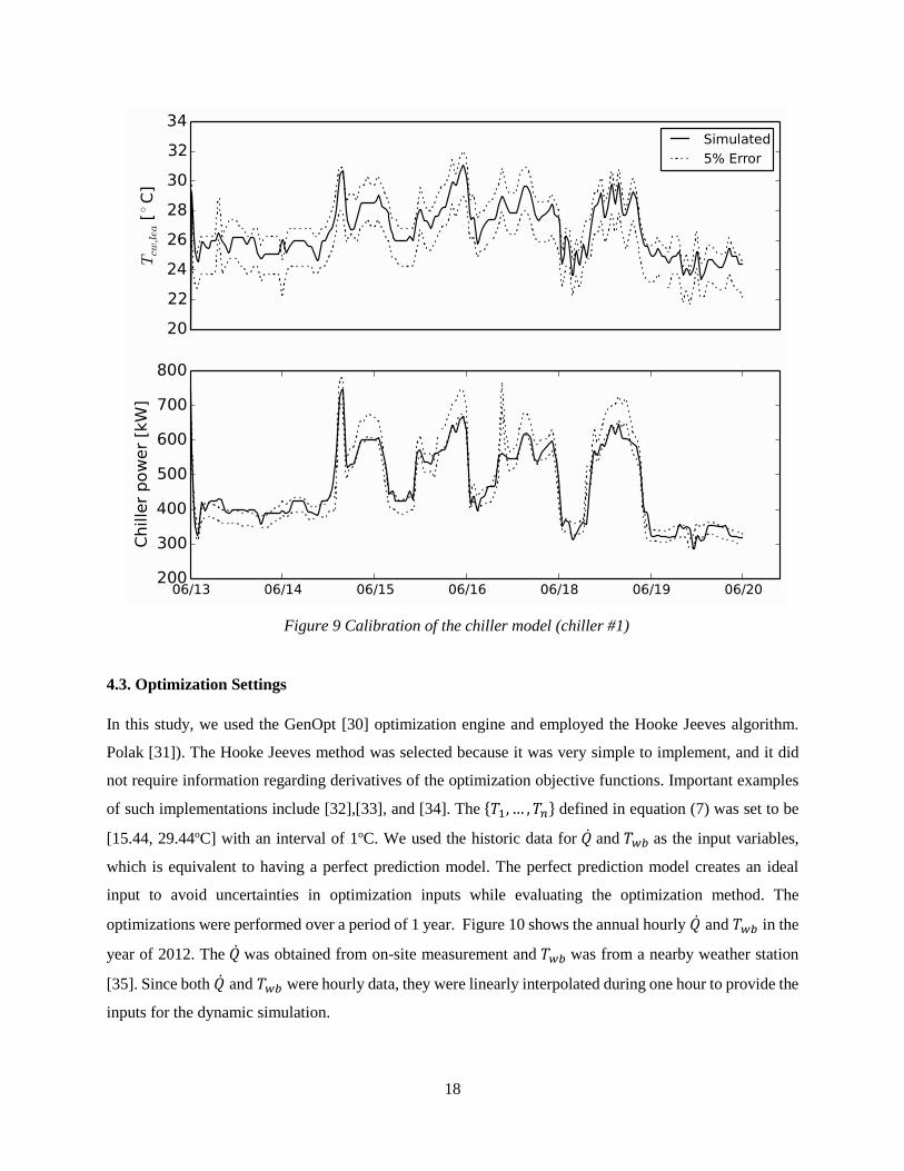
chilled water temperature. Figure 9 shows the calibration result of chiller #1 for one week in 2012. The

calibrated model can predict a close result for the temperature of the condenser water leaving the chiller,

𝑇𝑐𝑤,𝑙𝑒𝑎, and the chiller power since the relative errors of most of the predictions are less than 5%.

AllOff

OneOn

TwoOn

T1

T2

T4

T6

{0,1,2,3}

else: 0.0

multiSwitch

ThreeOn

T3

T5

replicator combiTable1D

CooLoa

y

18

Figure 9 Calibration of the chiller model (chiller #1)

4.3. Optimization Settings

In this study, we used the GenOpt [30] optimization engine and employed the Hooke Jeeves algorithm.

Polak [31]). The Hooke Jeeves method was selected because it was very simple to implement, and it did

not require information regarding derivatives of the optimization objective functions. Important examples

of such implementations include [32],[33], and [34]. The {𝑇1, … , 𝑇𝑛} defined in equation (7) was set to be

[15.44, 29.44oC] with an interval of 1oC. We used the historic data for �̇� and 𝑇𝑤𝑏 as the input variables,

which is equivalent to having a perfect prediction model. The perfect prediction model creates an ideal

input to avoid uncertainties in optimization inputs while evaluating the optimization method. The

optimizations were performed over a period of 1 year. Figure 10 shows the annual hourly �̇� and 𝑇𝑤𝑏 in the

year of 2012. The �̇� was obtained from on-site measurement and 𝑇𝑤𝑏 was from a nearby weather station

[35]. Since both �̇� and 𝑇𝑤𝑏 were hourly data, they were linearly interpolated during one hour to provide the

inputs for the dynamic simulation.

19

(a)

(b)

Figure 10 Input data for the optimziation (a) cooling load (b) wet bulb temperature

20

To evaluate the impact of the optimization frequency on the energy savings from the condenser water set

point optimization, we performed optimizations with three different frequencies: once an hour (Hourly

OPT), once a day (Daily OPT) and once a week (Weekly OPT) using historic data as perfect predictions of

�̇� and 𝑇𝑤𝑏. An exhaustive search method with a frequency as once an hour (Hourly ES) was used as the

benchmark.

The optimizations were performed using a Dell Precision T7600 Tower Workstation computer with a Four

Core XEON processor (E5-2609, 2.4GHz, 10M, 6.4 GT/s). The operation system is Windows 7 Ultimate.

4.4. Evaluation of Starting Point Selection Methods

In this section, we evaluated the performances of four different starting point selection methods. The four

methods are: approach temperature, middle point, previous value, and high point. All the four methods are

implemented in Hourly OPT.

Table 1 shows the accuracy of the optimization with four starting point selection methods compared with

the Hourly ES. There are 8,760 searches performed for the hourly optimization over a year. None of the

starting point selection methods could guarantee the global minimum for all searches. With a better starting

point, the search using the approach temperature method could mitigate the local minima problem and had

the lowest failure point ratio (the ratio of number of failure searches in finding global optimal to the total

number of searches). This means the accuracy of the simple estimation on the approach temperature doesn’t

significantly impact the searching of the optimal results in this study. The failure ratio of the middle point

method and the high point method were about twice of the approach temperature method. The previous

value method experienced the highest failure rate, which is more than three times compared to the approach

temperature method. This means that the search with the previous value method is more likely trapped by

local minima. However, it is surprising that the energy saving penalties for the failures were significantly

smaller compared to the searching failure ratios.

21

Table 1 Comparison of the accuracy using different starting point selection methods

Approach

Temperature High Point

Previous

Value Middle Point

Benchmark

(Exhaustive

Search)

Number of

Failure

Searches

315 814 1,080 715 N/A

Failure

Search Ratio 3.59% 9.27% 12.30% 8.14% N/A

Annual

Energy

Consumption

[kWh]

5,028,148 5,030,700 5,030,545 5,028,436 5,027,758

Annual

Energy

Saving Ratio

9.67% 9.63% 9.63% 9.67% 9.68%

Table 2 compares the computational performances of four methods. Depending on the starting point

selection methods, the number of simulations needed by the optimization arranges from 30,989 to 52,285

which is significantly less than 113,658 simulations required by the exhaustive search. In terms of the

computing time, the previous value method had the best performance and it reduced the number of

simulations by around 72.73% and computing time by about 55.74% compared to the exhaustive search.

The approach temperature method had similar performance as the previous value method. The high point

method and the middle point method had lower reduction ratios for both the number of simulation (54.00%-

57.82%) and computing time (40.40% - 42.25%).

Table 2 Comparison of the computational performance using different starting point selection methods

Approach

Temperature High Point

Previous

Value Middle Point

Exhaustive

Search

Number of

Simulation 34,585 52,285 30,989 47,941 113,658

Number of

Simulation

Reduction

Ratio

69.57% 54.00% 72.73% 57.82% N/A

Computing

Time [s] 25,045 32,933 24,459 31,914 55,258

Computing

Time

Reduction

Ratio

54.68% 40.40% 55.74% 42.25% N/A

22

It is worth mentioning that the average CPU time for each hourly optimization is around 2.86-6.31s, which

is significantly less than the optimization period. Thus, we believe that the model and the optimization is

fast enough to perform optimization more frequently.

To get more insights on when and why each method failed to find the global minimum, we studied four

different scenarios. The first scenario happened when �̇� or 𝑇𝑤𝑏 was low. In this scenario, the flat range was

likely to occur at the high end. As shown in Figure 11 (a), the flat range was between 27.44oC and 29.44oC.

Since the high point method selected 𝑇𝑐𝑤,𝑠𝑒𝑡,𝐻 as 29.44oC, it was trapped by the local minima within the

flat range. Other methods selected a starting point outside the flat range and successfully found the global

minimum.

The second scenario occurred when �̇� was extremely low. This could happen in the winter that the chiller

was still running to provide cooling for building internal zones, such as computer rooms, even 𝑇𝑤𝑏 is very

low. The flat range extended to a very low temperature (Figure 11(b)) and both the middle point method

and high point method failed to find the global minimum.

The third scenario happened when 𝑇𝑤𝑏 < 𝑇𝑤𝑏,𝑛𝑜𝑚 and �̇� was relatively high. As mentioned earlier,

equation (19) may underestimate 𝑇𝑐𝑤,𝑙𝑜𝑤. In that case, the approach temperature method will get stuck in

the local minima. For instance, in Figure 11 (c), 𝑇𝑐𝑤,𝑠𝑒𝑡,𝑠𝑡𝑎 given by equation (19) was 24.44oC, which was

still in the flat range of [21.44, 24.44oC]. Since the initial search step is 2.00oC, the optimization algorithm

found that both 𝑇𝑐𝑤,𝑠𝑒𝑡 = 22.44oC and 26.44oC cause a higher energy consumption than 𝑇𝑐𝑤,𝑠𝑒𝑡 = 24.44oC,

but missed the global minimum at 25.44oC. In this case, using a smaller initial search step, such as 1.00oC

may avoid the problem. However, this is at the cost of longer searching time.

The fourth scenario appeared when the difference between the optimal 𝑇𝑐𝑤,𝑠𝑒𝑡 for the adjacent optimization

periods was significant. This made the previous value method fail to reach the global minimum. As shown

in Figure 11 (d), the previous value method was stuck at 22.44oC, which was the optimal 𝑇𝑐𝑤,𝑠𝑒𝑡 for the

previous optimization period.

23

(a)

(b)

(c)

(d)

Figure 11 The scenarios when different starting point selection methods failed to find the global

minmum

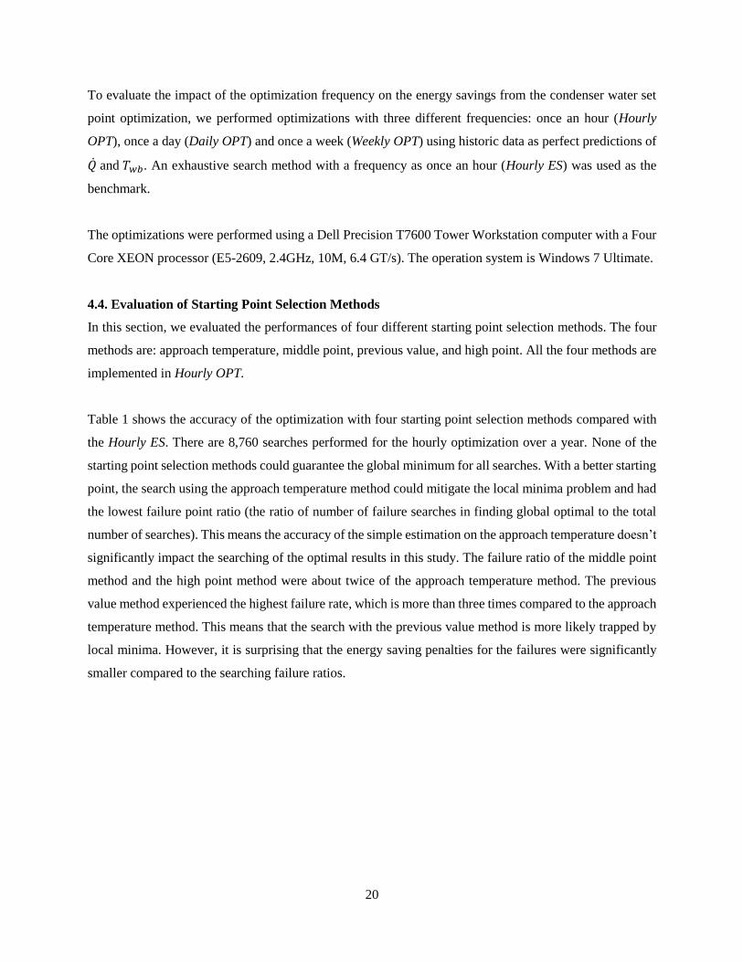
To understand why relatively large searching failure ratios only led to small differences in energy savings,

we analyzed the energy saving penalty due to failures in identifying the optimal condenser water set point.

Based on Figure 12, for all the methods, more than 90% of the energy saving penalties are less than 5%.

As shown in Figure 11, the energy saving penalties can be as low as 0.20%. Thus, although the searching

failure ratios of those methods are up to 12.30%, the impact of the searching failures on the total energy

savings is not quite significant.

24

Figure 12 The energy saving penalty due to the failure in predicting the optimal condenser water set

point

4.5 Evaluation of the Impact of the Optimization Frequency on the Energy Saving

To model the uncertainties in the load and weather prediction due to long prediction horizons (one day and

one week), we used the following equation to generate the synthetic errors:

�̇�∗ = �̇� + 𝑟𝑎𝑛𝑑𝑜𝑚(−Δ�̇� , Δ�̇�), (27)

𝑇𝑤𝑏∗ = 𝑇𝑤𝑏 + 𝑟𝑎𝑛𝑑𝑜𝑚(−Δ𝑇𝑤𝑏 , Δ𝑇𝑤𝑏) + 𝑇𝑠𝑡𝑎𝑒𝑟𝑟, (28)

where �̇�∗ and 𝑇𝑤𝑏∗ are the predicted cooling load and wet bulb temperature with errors. 𝑇𝑠𝑡𝑎𝑒𝑟𝑟 is the static

error occurs in the wet bulb temperature prediction. For the hourly optimization, we assumed Δ�̇� = 0 W,

Δ𝑇𝑤𝑏 = 0 K, and 𝑇𝑠𝑡𝑎𝑒𝑟𝑟 = 0 K so that we could use the results of the Hourly OPT as the benchmark for

comparison. For the daily optimization, Δ�̇� = 20%�̇�𝑛𝑜𝑚 , Δ𝑇𝑤𝑏 = 1 K, and 𝑇𝑠𝑡𝑎𝑒𝑟𝑟 = 1 K respectively.

For the weekly optimization, Δ�̇� = 40%�̇�𝑛𝑜𝑚 , Δ𝑇𝑤𝑏 = 2 K and Δ𝑇𝑤𝑏 = 0 K, and 𝑇𝑠𝑡𝑎𝑒𝑟𝑟 = 1 K. The

𝑟𝑎𝑛𝑑𝑜𝑚(𝑎, 𝑏) is a function that returns a random value between the input range [a, b]. A daily optimization

and a weekly optimization using the above inputs were named Daily OPT with Error and Weekly OPT with

Error, respectively. The approach temperature starting point selection method was applied in all

optimizations.

Table 3 compares the performance of the optimization with different optimization frequencies. The Hourly

OPT provided almost the same solution as the Hourly ES with about half of the computing time. By further

reducing the number of optimizations, the Daily OPT and the Weekly OPT achieved an around 95.00% time

25

and 97.00% reduction in computing time with only 0.07% and 0.09% penalty in predicted energy saving

than the Hourly ES, respectively. Compared to the Hourly OPT, the Daily Opt and the Weekly OPT were

about 10 times and 15 times faster and provides energy savings of only 0.07% less. The reason why the

Daily Opt and the Weekly OPT did not achieve 24 times and 168 times faster than the Hourly OPT is

because the daily and weekly simulation cost more time to solve than the hourly simulation. Even with

uncertainties in the �̇� and 𝑇𝑤𝑏 prediction, the Daily OPT with Error and the Weekly OPT with Error got a

similar energy savings compared to the Daily OPT and the Weekly OPT.

Table 3 Perforamnces of different optimization frequencies

Hourly

OPT Daily OPT

Daily OPT

with Error Weekly OPT

Weekly OPT

with Error

Annual Energy

Consumption [kWh] 5,028,148 5,031,571 5,031,752 5,032,502 5,032,199

Energy Saving Ratio 9.67% 9.60% 9.60% 9.58% 9.59%

Computing Time [s] 25,045 2,536 2,796 1,658 1,912

Computing Time

Reduction Ratio 54.68% 95.41% 94.94% 97.00% 96.54%

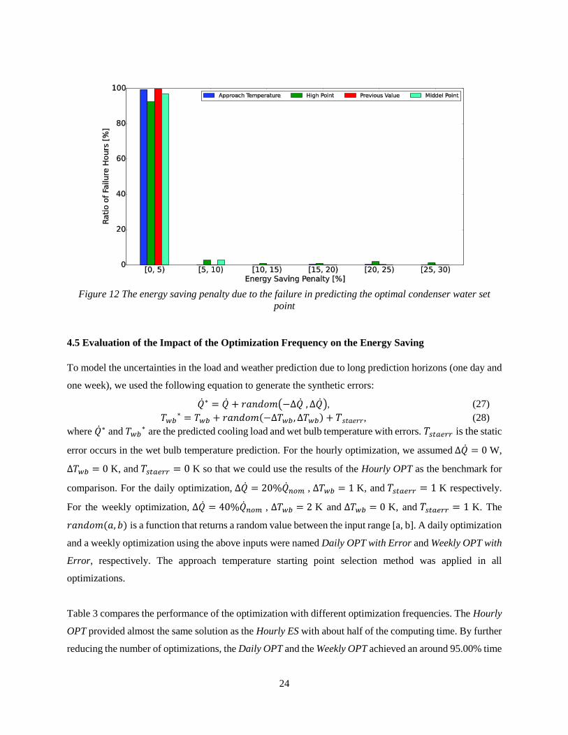
To understand why the impact of the optimization frequency on the energy savings is not significant, we

investigated the profiles of the inputs for the condenser water set point optimization. Figure 13 shows the

distribution of the daily and weekly standard deviations in the wet bulb temperature in Washington D.C. in

2012. The standard deviations in the wet bulb temperature of all the days and the weeks are less than 6.00oC.

This means the weather of the studied period (year of 2012) in Washington D.C. is relatively temperate

with a small variation in the wet bulb temperature. We then looked at the cooling load distribution, since

there are different cooling load profiles for different seasons in the cooling period, we selected two typical

days with different cooling load profiles: one day is from the mild season (April 20th, Friday) and the other

day is from the hot season (July 20th, Friday). Both the mild day and the hot day have the daily standard

deviation in the wet bulb temperature less than 6.00oC.

26

Figure 13 The distribution of the standard deviations for the wet bulb temperature of Washington

D.C. in 2012

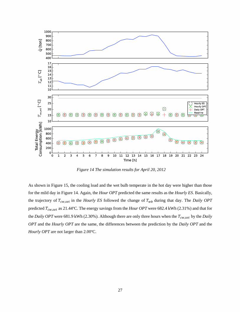
For the mild day, the cooling load changed from around 400 ton to 900 ton and the wet bulb temperate was

from 11.00oC to 16.00oC (Figure 14). The Hourly OPT predicted the same results as the Hourly ES and a

2,648 kWh (16.14%) energy saving was achieved. The Daily OPT produced a slightly different result with

energy savings of 16.13%. The 𝑇𝑐𝑤,𝑠𝑒𝑡 was constant as 15.44oC from 0:00 to 13:00 because of the low wet

bulb temperate. The 𝑇𝑐𝑤,𝑠𝑒𝑡 began to increase at 14:00 after 𝑇𝑤𝑏 passed 15.00oC. At around 17:00, 𝑇𝑐𝑤,𝑠𝑒𝑡

suddenly raised to 20.44oC. The reason for the quick increase is that at 17:00, the cooling load decreased

from 900 ton to 731 ton and the number of operating chillers reduced from 2 to 1. As a result, the cooling

load was met by the remained operating chillers. With the increased cooling load, it took more effort for

the dedicated cooling tower to cool the condenser water to the given 𝑇𝑐𝑤,𝑠𝑒𝑡, which makes the optimal

𝑇𝑐𝑤,𝑠𝑒𝑡 increase. After 17:00, 𝑇𝑐𝑤,𝑠𝑒𝑡 began to decrease to reflect the reduced cooling load. It returned to

15.44oC at 19:00 and remained unchanged for the rest time. The Daily OPT predicted 𝑇𝑐𝑤,𝑠𝑒𝑡 as 15.44oC

and there are only four hours when the 𝑇𝑐𝑤,𝑠𝑒𝑡 by the Daily OPT and the Hourly OPT was different.

27

Figure 14 The simulation results for April 20, 2012

As shown in Figure 15, the cooling load and the wet bulb temperate in the hot day were higher than those

for the mild day in Figure 14. Again, the Hour OPT predicted the same results as the Hourly ES. Basically,

the trajectory of 𝑇𝑐𝑤,𝑠𝑒𝑡 in the Hourly ES followed the change of 𝑇𝑤𝑏 during that day. The Daily OPT

predicted 𝑇𝑐𝑤,𝑠𝑒𝑡 as 21.44oC. The energy savings from the Hour OPT were 682.4 kWh (2.31%) and that for

the Daily OPT were 681.9 kWh (2.30%). Although there are only three hours when the 𝑇𝑐𝑤,𝑠𝑒𝑡 by the Daily

OPT and the Hourly OPT are the same, the differences between the prediction by the Daily OPT and the

Hourly OPT are not larger than 2.00oC.

28

Figure 15 The simulation results for July 20, 2012

Based on the above analysis, we can see that despite of different cooling load profiles, the lower daily

deviation in the wet bulb temperature makes the difference between the predictions by the Daily OPT and

the Hour OPT not obvious.

Similarly, the wet bulb temperature does not change significantly over a week so that the Weekly OPT could

achieve similar performance to the Daily OPT. The standard deviations for the weeks, to which April 20

and July 20 belong, are 3.36oC and 1.81oC, respectively. As a result, the predictions by the Weekly OPT for

the two weeks are 15.44oC and 24.44 oC, which are both close to the results by the Daily OPT for April 20

and July 20, respectively.

29

5. Conclusion

In this paper, we proposed an operational support system to improve the operational efficiency of condenser

water loops in legacy chiller plants. We evaluated how different starting point selection methods and the

optimization frequency affect the condenser water set point optimization results via a case study. Based on

the results of the case study, the following conclusions can be drawn:

1) The proposed system can achieve significant energy savings for the studied chiller plant. The

annual energy saving ratio is up to around 9.67%. It should be noted that the energy savings is

reached without adding new equipment or requiring significant efforts for implementation.

2) Optimization starting point selection does not significantly impact energy savings from the

condenser water set point optimization for the studied chiller plant significantly, although it does

impact the computing time and the failure rate on finding the global optimum. The previous value

method can achieve the fastest search but it also obtains the largest failure number. The approach

temperature method is promising since it has a failure rate 2-3 times lower than other methods. The

computing time of the approach temperature method is almost the same as the previous value

method.

3) The optimization frequency doesn’t significantly affect the energy savings from the condenser

water set point optimization for the studied chiller plant. This is because the daily and weekly

variation in the wet bulb temperature is not very large for the site in the studied year, which leads

to small differences between the predictions of the optimal condenser water set point with different

optimization frequencies.

In this paper, we demonstrated the performance of the operational support system via a single chiller plant

with one type of climate condition. It will be interesting to perform more simulations to access the energy

saving potential of this approach for different plant configurations, cooling loads, and climates in the future

work. As a pilot study, we manually developed the dedicated model for the studied plant and calibrated the

models according to the measured data. To enable the large scale application, it is worth investigating how

to automatize the procedure for creating and calibrating the chiller plant models so that the efforts for

implementation can be minimized.

30

Acknowledgement

This research was supported by the U.S. Department of Defense under the ESTCP program. The authors

thank Marco Bonvini, Michael Wetter, Mary Ann Piette, Jessica Granderson, Oren Schetrit, Rong Lily Hu

and Guanjing Lin for the support provided through the research.

This research also emerged from the Annex 60 project, an international project conducted under the

umbrella of the International Energy Agency (IEA) within the Energy in Buildings and Communities (EBC)

Programme. Annex 60 will develop and demonstrate new-generation computational tools for building and

community energy systems based on Modelica, Functional Mockup Interface and BIM standards.

Reference

[1] Westphalen D, Koszalinski S. Energy Consumption Characteristics of Commercial Building HVAC

Systems Volume I : Chillers, Refrigerant Compressors,and Heating Systems. Arthur D. Little, Inc.; 2001.

[2] ASHRAE. ASHRAE Handbook HVAC Application. Atlanta: ASHRAE, Inc.; 2011.

[3] Braun JE, Klein SA, Mitchell JW, Beckham WA. Application of optimal control to chilled water

systems without storage. ASHRAE Trans 1989;95(1):663-75.

[4] Hydeman M, Zhuo G. Optimizing Chilled Water Plant Control. ASHRAE J 2007;54(3):56-74.

[5] Sun J, Reddy A. Optimal Control of Building HVAC&R Systems using Complete Simulation-based

Sequential Quadratic Programming (CSB-SQP). Build Environ 2005;40(5):657-69.

[6] Yu FW, Chan KT. Optimization of Water-cooled Chiller System with Load-based Speed Control.

Appl Energ 2008;85(2008):931-50.

[7] Zhang Z, Li H, Turner WD, Deng S. Optimization of the Cooling Tower Condenser Water Leaving

Temperature using a Component-based Model. ASHRAE Trans 2011;117(1):934-44.

[8] Malara ACL, Huang S, Zuo W, Sohn MD, Celik N. Optimal Control of Chiller Plants using Bayesian

Network. In: Proceedings of The 14th International Conference of the IBPSA Hyderabad, 2015. p. 449-

55.

[9] Lu L, Cai W, Soh YC, Xie L, Li S. HVAC System Optimization - Condenser Water Loop. Energ

Convers Manage 2004;45(4):613-30.

[10] Ma Z, Wang S, Xu X, Xia F. A Supervisory Control Strategy for Building Cooling Water Systems

for Practical and Real Time Applications. Energ Convers Manage 2008;49(8):2324-36.

[11] Lee KP, Cheng TA. A Simulation–optimization Approach for Energy Efficiency of Chilled Water

System. Energ Buildings 2012;54(2012):290-6.

[12] Huang S, Zuo W. Optimization of the Water-cooled Chiller Plant System Operation. In: Proceedings

of ASHRAE/IBPSA-USA Building Simulation Conference, Atlanta, GA, U.S.A., 2014. p. 300-7.

[13] Ma Y, Borrelli F, Hencey B, Coffey B, Bengea S, Haves P. Model Predictive Control for the

Operation of Building Cooling Systems. IEEE Trans Control Syst Technol 2010;20(3):796 - 803.

[14] Lazos D, Sproul A, Ka M. Development of Hybrid Numerical and Statistical Short Term Horizon

Weather Prediction Models for Building Energy Management Optimisation. Build Environ;90(2015):82-

95.

31

[15] Huang S, Zuo W, Sohn MD. A Bayesian Network Model for Predicting the Cooling Load of

Educational Facilities. In: Proceedings of ASHRAE and IBPSA-USA SimBuild 2016 Building

Performance Modeling Conference, Salt Lake City, UT, 2016.

[16] Hassin R, Henig M. Dichotomous Search for Random Objects on an Interval. Math Oper Res

1984;9(2):301-8.

[17] Eiselt HA, Sandblom. Linear Programming and its Applications. 2007 ed. Berlin: Springer-Verlag

Berlin Heidelberg; 2007.

[18] Fernandes FP, Costa MFP, Fernandes EMGP, Rocha AMAC. Multistart Hooke and Jeeves Filter

Method for Mixed Variable Optimization. In: Proceedings of the 11th international conference of

numerical analysis and applied mathematics Rhodes, Greece, 2013. p. 614-7.

[19] Gyorgy A. Efficient Multi-start Strategies for Local Search Algorithms. J Artif Intell Res

2011;41(2011):407-44.

[20] Kelman A, Ma Y, Borrelli F. Analysis of Local Optima in Predictive Control for Energy Efficient

Buildings. J Build Perform Simu 2012;6(3):236–55.

[21] Sutherland JW. Analysis of Mechanical Draught Counterflow Air/Water Cooling Towers. J Heat

Transfer 1983;105(3):576-83.

[22] Braun JE, Klein SA, Mitchell JW. Effectiveness Models for Cooling Towers and Cooling Coils.

ASHRAE Trans 1989;95(2):164-74.

[23] Schwedler M. Effect of Heat Rejection Load and Wet Bulb on Cooling Tower Performance.

ASHRAE J 2014;56(1):16-22.

[24] Wetter M, Zuo W, Nouidui T, Pang X. Modelica Buildings library. J Build Perform Simu

2014;7(4):253-70.

[25] Nouidui TS, Phalak K, Zuo W, Wetter M. Validation of the Window Model of the Modelica

Buildings Library. In: Proceedings of the 9th International Modelica Conference, Munich, Germany,

2012. p. 727-36.

[26] Zuo W, Wetter M, Li D, Jin M, Tian W, Chen Q. Coupled Simulation of Indoor Enviroment, HVAC

and Control System by using Fast Fluid Dynamics and the Modelica Buildings Library. In: Proceedings

of ASHRAE/IBPSA-USA Building Simulation Conference, Atlanta, GA, U.S.A., 2014. p. 56-63.

[27] Otter M, Årzén K-E, Dressler I. StateGraph - a Modelica Library for Hierarchical State Machines. In:

Proceedings of the 4th International Modelica Conference, Hamburg, Germany, 2005. p. 569-78.

[28] Dassault Systems. Dymola. <http://www.3ds.com/products-services/catia/capabilities/modelica-

systems-simulation-info/dymola> (accessed

[29] Input Output Reference: the Encyclopedic Reference to EnergyPlus Input and Output.

<http://apps1.eere.energy.gov/buildings/energyplus/pdfs/inputoutputreference.pdf> (accessed May 14.

2015).

[30] Wetter M. GenOpt - a Generic Optimization Program. In: Proceedings of the 7th IBPSA Conference,

Rio de Janeiro, Brazil, 2001. p. 601-8.

[31] Polak E. Optimization. Algorithms and consistent approximations. Appl Math Sci 1997;124(

[32] Wetter M, Polak E. Building design optimization using a convergent pattern search algorithm with

adaptive precision simulations. Energ Buildings 2005;37(6):603-12.

[33] Coffey B. Approximating model predictive control with existing building simulation tools and offline

optimization. J Build Perform Simu 2013;6(3):220-35.

[34] Bagirov AM, Barton AF, Mala-Jetmarova H, Nuaimat AA, Ahmed ST, Sultanova N, et al. An

algorithm for minimization of pumping costs in water distribution systems using a novel approach to

pump scheduling. Mathematical and Computer Modelling 2013;67(3-4):873-86.

[35] National Climatic Data Center. Quality Controlled Local Climatological Data.

<http://www.ncdc.noaa.gov/data-access/land-based-station-data/land-based-datasets/quality-controlled-

local-climatological-data-qclcd> (accessed May 14. 2015).