Contents lists available at SciVerse ScienceDirect
Powder Technology
j ourna l homepage: www.e lsev ie r .com/ locate /powtec
Improved digital image analysis technique for the evaluation of segregation inpseudo-2D beds
O.O. Olaofe a, K.A. Buist a, N.G. Deen a,⁎, M.A. van der Hoef a,b, J.A.M. Kuipers a
a Eindhoven University of Technology, Chemical Engineering and Chemistry Dept., PO Box 513, 5600 MB Eindhoven, The Netherlandsb University of Twente, Faculty of Science and Technology, PO Box 217, 7500 AE Enschede, The Netherlands
In addition to information on the behavior of bubbles, the dynamics of mixing and segregation is often re-quired because of its importance in describing physical and chemical processes involving fluidized suspen-sions. In this work, the enhanced capacities of state-of-the-art photographic instruments have beenadopted in a new Digital Image Analysis (DIA) technique for the evaluation of local compositions and degreesof segregation in lab-scale pseudo-2D gas–solid fluidized beds. Furthermore, the newly developed imageanalysis technique permits the simultaneous evaluation of bed height and bubble size and position. The ex-tent of mixing and segregation for polydisperse systems can be determined more accurately when the differ-ent particle species are classified by distinct colors. The reproducibility of lab measurements was found to besatisfactory, and the extents of segregation in snapshots of a Discrete Element Method (DEM) simulation,evaluated using the new technique, were found to be in good agreement with exact values calculated fromindividual particle positions in the DEM.
In the past couple of decades, there has been a dramatic increasein the capacity of computer processors making it possible to success-fully simulate complex systems. However, in order to fully validatethe models used in these simulations there is the increasing need toget accurate and detailed quantitative experimental data.
Over the years, different techniques for probing the dynamics offluidized bed have been developed. These techniques generally fallinto one of two main categories: intrusive or non-intrusive tech-niques. The intrusive techniques are largely based on resistance, im-pedance, inductance, piezoelectric or thermal probes while thenon-intrusive techniques are mostly based on photographic, X-ray,light scattering or laser techniques [1]. The intrusive techniques, tosome extent, however, interfere with the dynamics of beds, unlikethe non-intrusive techniques.
In recent years, the advances in digital imaging systems and pro-cessing have led to an increase in the application of photography inthe study of lab-scale fluidized beds. It is particularly suitable forpseudo-2D gas–solid systems where the inter-phase boundary iseasy to detect and the effect of bed depth is minimal.
Caicedo et al. [2] used data collected from a CCD camera to deter-mine the influence of reduced velocity on the shape factor and aspectratio of bubbles formed in a 2D fluidized bed. Lim et al. [3] investigat-ed the distributions of bubble pierced length as well as some other
rights reserved.
bubble size measures, experimentally, by employing Digital ImageAnalysis methods. Hull et al. [4] developed semi-empirical correla-tions for the average size and rise velocity of bubbles in a2D-bubbling fluidized bed, with and without simulated horizontaltube bundles, using digitized images captured with a CCD camera.Goldschmidt et al. [5] developed a whole-field, non-intrusive, DigitalImage Analysis technique to study the dynamics and segregationrates in pseudo-2D dense gas-fluidized beds. In their work, a 3-CCDcolor camera was used to demonstrate that, using binary mixture ofparticles, the local mixture composition could be determined within10% accuracy. Furthermore, they showed that even small bubblesand voidage waves could be detected with their technique. However,by working with a camera of limited capacity and by carrying out theimage processing directly in the RGB color spectrum, the accuracy oftheir technique was rather limited. Shen et al. [6], using the imageprocessing toolbox of Matlab achieved a high level of automationin the acquisition, processing and analysis of digitized images oftwo-dimensional bubbling fluidized beds captured with a digitalvideo camera. They used the time-average data from the images toobtain bubble diameter, velocity, bubble number density and gasthroughflow. Bokkers et al. [7] substituted the fluid seeds in PIVwith bed particles to obtain particle velocity fields in 2D fluidizedbed experiments monitored with a monochrome high-speed digitalcamera. An image analysis technique, based on the computation ofthe cross correlation of bubble images with multiple spatial resolu-tions, was proposed by Cheng et al. [8] for measuring the bubblevelocity fields at high bubble number density in two dimensionalswarms. In their work, the PIV algorithm gave better results, compared
to several PTV schemes, because of its robustness in measuring the op-tical and dynamic characteristics of bubbles.
Some works have extended the application of photography to 3Dbeds. Zhu et al. [9] determined the size distribution of nano-particleagglomerates at the top of a cylindrical fluidized bed after analyzingthe images captured with a CCD camera. Also, Wang et al. [10] usedlaser-based planar imaging, with the aid of a high-resolution digitalCCD camera, to determine the shape and size of aggregates innano-particle fluidization experiment carried out in a column withrectangular cross-section.
In addition to information on the dynamics of bubbles, the dynam-ics of mixing and segregation is often desired. With the exception ofGoldschmidt et al. [5], none of the aforementioned works are ableto predict the time evolution of the extents of segregation in polydis-perse systems. In this work, the non-intrusive Digital Image Analysis(DIA) technique implemented by Goldschmidt et al. [5] was im-proved by utilizing a state-of-the-art photographic apparatus and anew image processing procedure to measure in-situ the degrees ofsegregation in polydisperse systems, particularly in binary and terna-ry systems, by differentiating colored particles by the unique colorthey express in pixels.
2. Experimental set-up
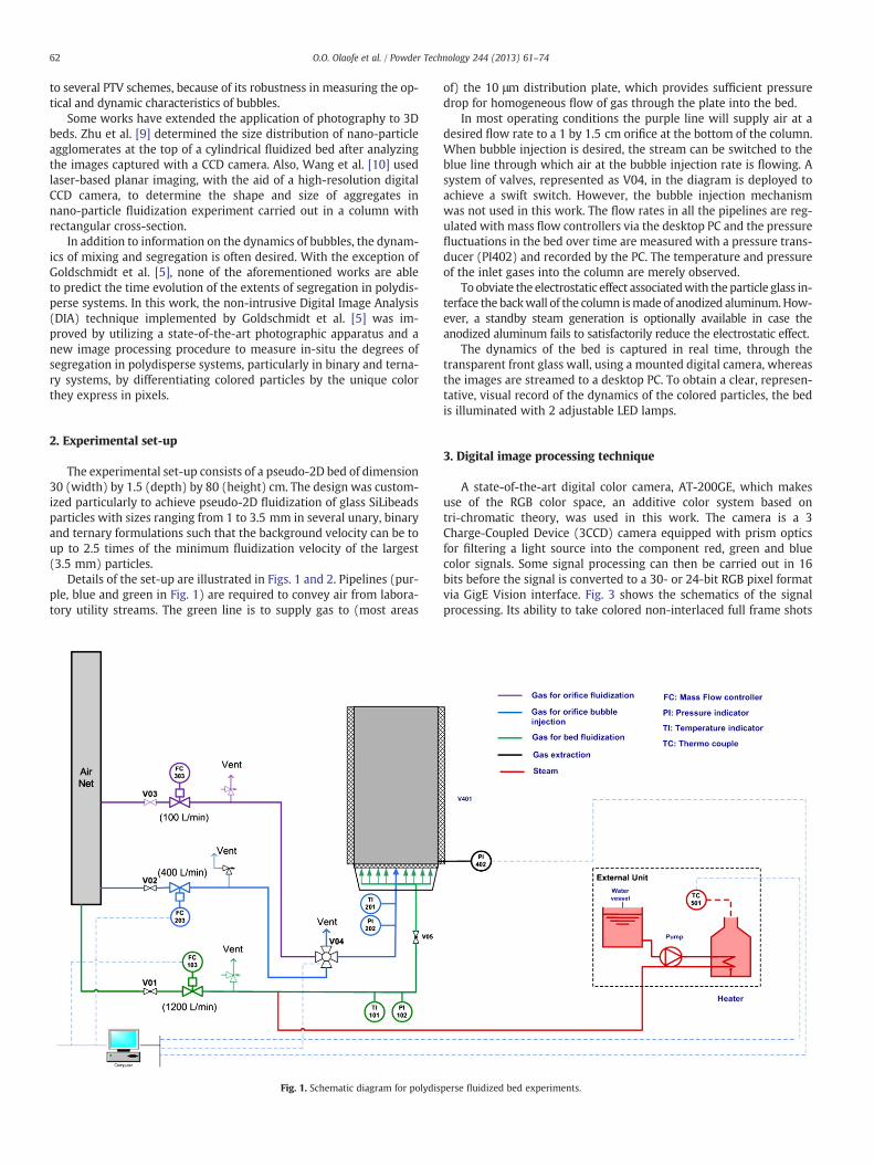
The experimental set-up consists of a pseudo-2D bed of dimension30 (width) by 1.5 (depth) by 80 (height) cm. The design was custom-ized particularly to achieve pseudo-2D fluidization of glass SiLibeadsparticles with sizes ranging from 1 to 3.5 mm in several unary, binaryand ternary formulations such that the background velocity can be toup to 2.5 times of the minimum fluidization velocity of the largest(3.5 mm) particles.
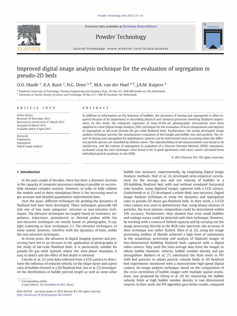
Details of the set-up are illustrated in Figs. 1 and 2. Pipelines (pur-ple, blue and green in Fig. 1) are required to convey air from labora-tory utility streams. The green line is to supply gas to (most areas
Fig. 1. Schematic diagram for polydis
of) the 10 μm distribution plate, which provides sufficient pressuredrop for homogeneous flow of gas through the plate into the bed.
In most operating conditions the purple line will supply air at adesired flow rate to a 1 by 1.5 cm orifice at the bottom of the column.When bubble injection is desired, the stream can be switched to theblue line through which air at the bubble injection rate is flowing. Asystem of valves, represented as V04, in the diagram is deployed toachieve a swift switch. However, the bubble injection mechanismwas not used in this work. The flow rates in all the pipelines are reg-ulated with mass flow controllers via the desktop PC and the pressurefluctuations in the bed over time are measured with a pressure trans-ducer (PI402) and recorded by the PC. The temperature and pressureof the inlet gases into the column are merely observed.
To obviate the electrostatic effect associatedwith the particle glass in-terface the backwall of the column ismade of anodized aluminum.How-ever, a standby steam generation is optionally available in case theanodized aluminum fails to satisfactorily reduce the electrostatic effect.
The dynamics of the bed is captured in real time, through thetransparent front glass wall, using a mounted digital camera, whereasthe images are streamed to a desktop PC. To obtain a clear, represen-tative, visual record of the dynamics of the colored particles, the bedis illuminated with 2 adjustable LED lamps.
3. Digital image processing technique
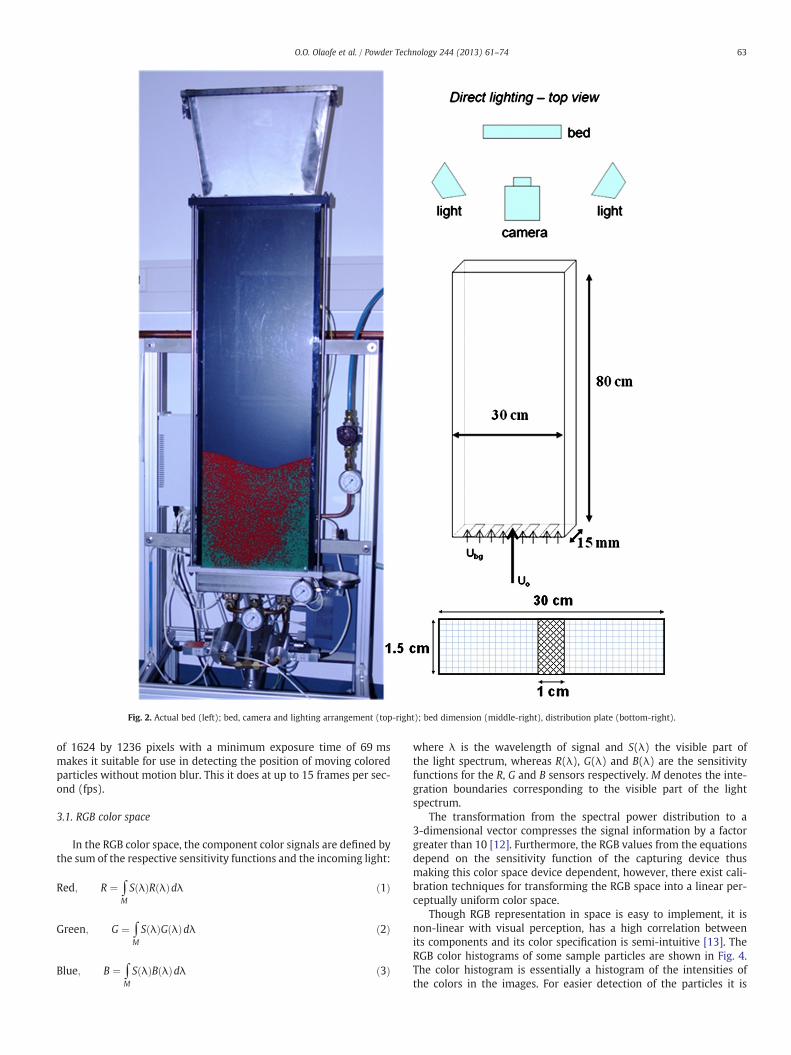
A state-of-the-art digital color camera, AT-200GE, which makesuse of the RGB color space, an additive color system based ontri-chromatic theory, was used in this work. The camera is a 3Charge-Coupled Device (3CCD) camera equipped with prism opticsfor filtering a light source into the component red, green and bluecolor signals. Some signal processing can then be carried out in 16bits before the signal is converted to a 30- or 24-bit RGB pixel formatvia GigE Vision interface. Fig. 3 shows the schematics of the signalprocessing. Its ability to take colored non-interlaced full frame shots
perse fluidized bed experiments.
Fig. 2. Actual bed (left); bed, camera and lighting arrangement (top-right); bed dimension (middle-right), distribution plate (bottom-right).
63O.O. Olaofe et al. / Powder Technology 244 (2013) 61–74
of 1624 by 1236 pixels with a minimum exposure time of 69 msmakes it suitable for use in detecting the position of moving coloredparticles without motion blur. This it does at up to 15 frames per sec-ond (fps).
3.1. RGB color space
In the RGB color space, the component color signals are defined bythe sum of the respective sensitivity functions and the incoming light:
Red; R ¼ ∫Μ
S λð ÞR λð Þdλ ð1Þ
Green; G ¼ ∫Μ
S λð ÞG λð Þdλ ð2Þ
Blue; B ¼ ∫Μ
S λð ÞB λð Þdλ ð3Þ
where λ is the wavelength of signal and S(λ) the visible part ofthe light spectrum, whereas R(λ), G(λ) and B(λ) are the sensitivityfunctions for the R, G and B sensors respectively. Μ denotes the inte-gration boundaries corresponding to the visible part of the lightspectrum.
The transformation from the spectral power distribution to a3-dimensional vector compresses the signal information by a factorgreater than 10 [12]. Furthermore, the RGB values from the equationsdepend on the sensitivity function of the capturing device thusmaking this color space device dependent, however, there exist cali-bration techniques for transforming the RGB space into a linear per-ceptually uniform color space.
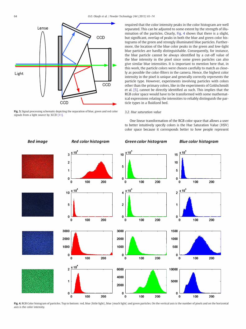
Though RGB representation in space is easy to implement, it isnon-linear with visual perception, has a high correlation betweenits components and its color specification is semi-intuitive [13]. TheRGB color histograms of some sample particles are shown in Fig. 4.The color histogram is essentially a histogram of the intensities ofthe colors in the images. For easier detection of the particles it is
required that the color intensity peaks in the color histogram are wellseparated. This can be adjusted to some extent by the strength of illu-mination of the particles. Clearly, Fig. 4 shows that there is a slight,but significant, overlap of peaks in both the blue and green color his-tograms of the green and strongly illuminated blue particles. Further-more, the location of the blue color peaks in the green and low-lightblue particles are hardly distinguishable. Consequently, for instance,the blue particle cannot be always identified by a cut-off value ofthe blue intensity in the pixel since some green particles can alsogive similar blue intensities. It is important to mention here that, inthis work, the particle colors were chosen carefully to match as close-ly as possible the color-filters in the camera. Hence, the highest colorintensity in the pixel is unique and generally correctly represents theparticle type. However, experiments involving particles with colorsother than the primary colors, like in the experiments of Goldschmidtet al. [5], cannot be directly identified as such. This implies that theRGB color space would have to be transformed with some mathemat-ical expressions relating the intensities to reliably distinguish the par-ticle types in a fluidized bed.
3.2. Hue saturation value
One linear transformation of the RGB color space that allows a userto better intuitively specify colors is the Hue Saturation Value (HSV)color space because it corresponds better to how people represent
t) and green particles. On the vertical axis is the number of pixels and on the horizontal
H ¼ 5þ B′ when R ¼ max R;G;Bð Þ; G ¼ min R;G;Bð Þ ð9Þ
H ¼ 1−G′ when R ¼ max R;G;Bð Þ; G≠min R;G;Bð Þ ð10Þ
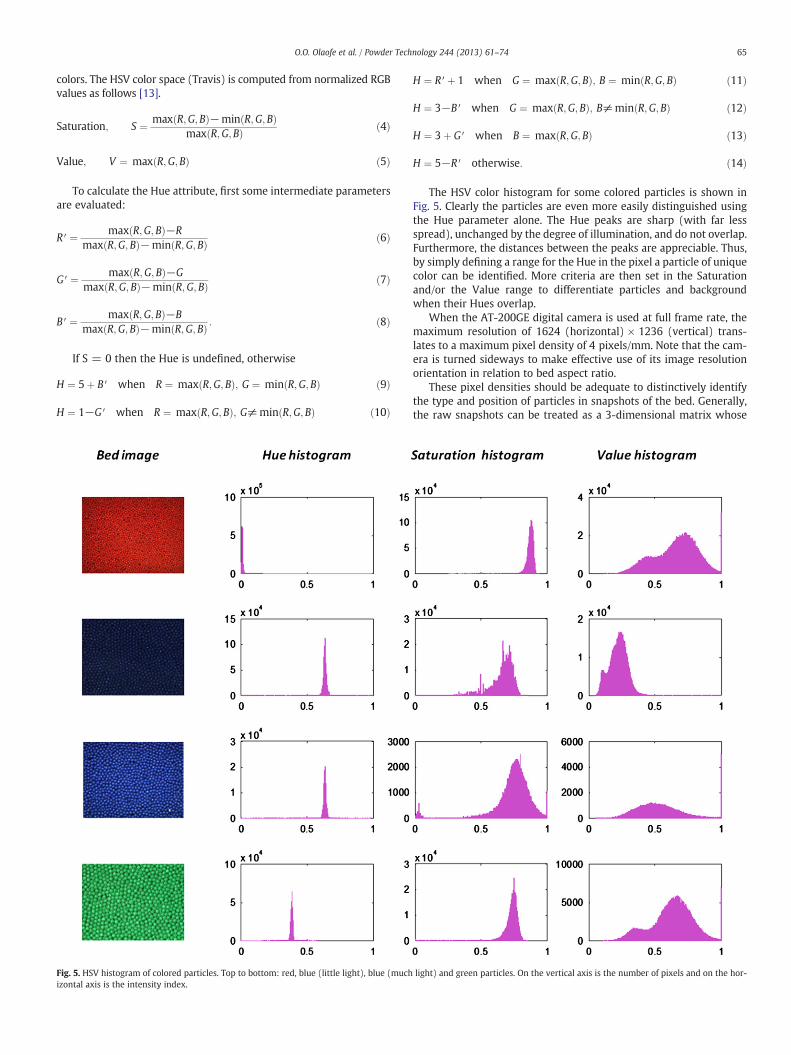
Fig. 5. HSV histogram of colored particles. Top to bottom: red, blue (little light), blue (muchizontal axis is the intensity index.
H ¼ R′þ 1 when G ¼ max R;G;Bð Þ; B ¼ min R;G;Bð Þ ð11Þ
H ¼ 3−B′ when G ¼ max R;G;Bð Þ; B≠min R;G;Bð Þ ð12Þ
H ¼ 3þ G′ when B ¼ max R;G;Bð Þ ð13Þ
H ¼ 5−R′ otherwise: ð14Þ
The HSV color histogram for some colored particles is shown inFig. 5. Clearly the particles are even more easily distinguished usingthe Hue parameter alone. The Hue peaks are sharp (with far lessspread), unchanged by the degree of illumination, and do not overlap.Furthermore, the distances between the peaks are appreciable. Thus,by simply defining a range for the Hue in the pixel a particle of uniquecolor can be identified. More criteria are then set in the Saturationand/or the Value range to differentiate particles and backgroundwhen their Hues overlap.
When the AT-200GE digital camera is used at full frame rate, themaximum resolution of 1624 (horizontal) × 1236 (vertical) trans-lates to a maximum pixel density of 4 pixels/mm. Note that the cam-era is turned sideways to make effective use of its image resolutionorientation in relation to bed aspect ratio.
These pixel densities should be adequate to distinctively identifythe type and position of particles in snapshots of the bed. Generally,the raw snapshots can be treated as a 3-dimensional matrix whose
light) and green particles. On the vertical axis is the number of pixels and on the hor-
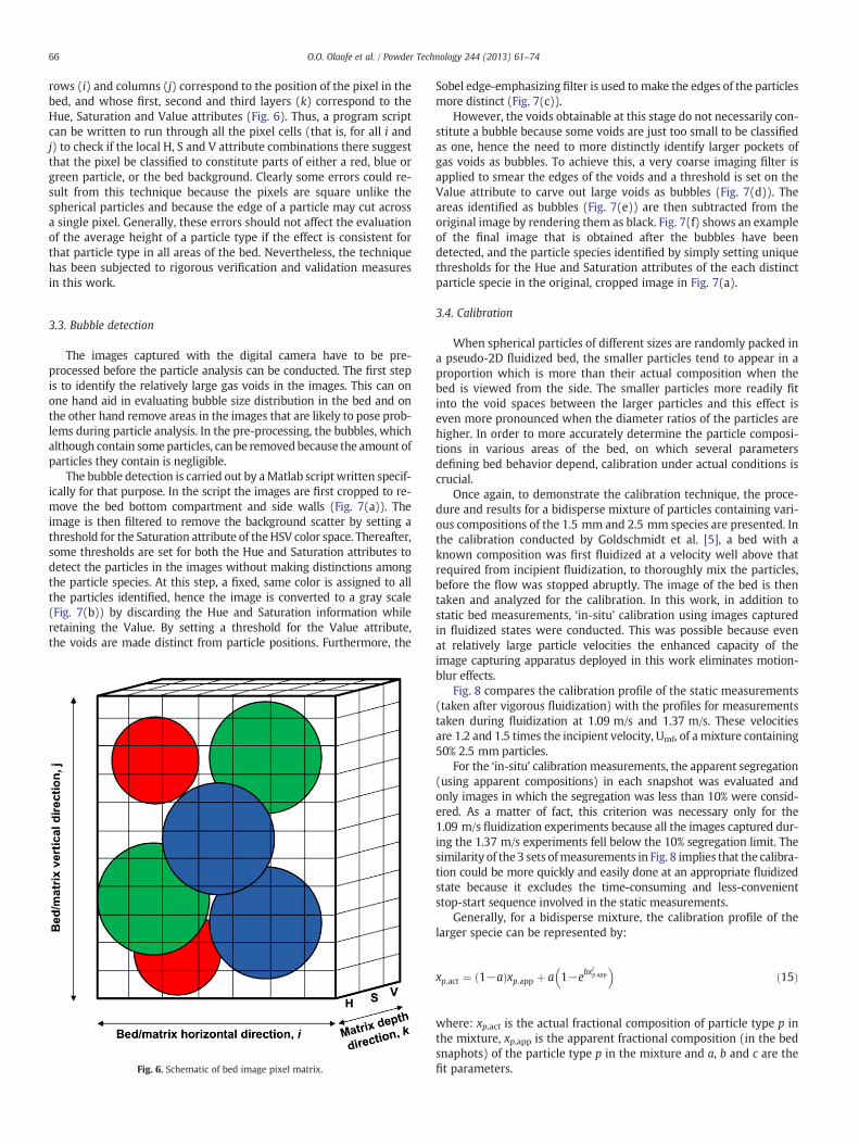
rows (i) and columns (j) correspond to the position of the pixel in thebed, and whose first, second and third layers (k) correspond to theHue, Saturation and Value attributes (Fig. 6). Thus, a program scriptcan be written to run through all the pixel cells (that is, for all i andj) to check if the local H, S and V attribute combinations there suggestthat the pixel be classified to constitute parts of either a red, blue orgreen particle, or the bed background. Clearly some errors could re-sult from this technique because the pixels are square unlike thespherical particles and because the edge of a particle may cut acrossa single pixel. Generally, these errors should not affect the evaluationof the average height of a particle type if the effect is consistent forthat particle type in all areas of the bed. Nevertheless, the techniquehas been subjected to rigorous verification and validation measuresin this work.
3.3. Bubble detection
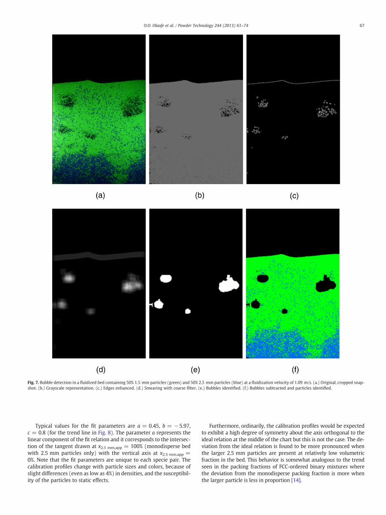
The images captured with the digital camera have to be pre-processed before the particle analysis can be conducted. The first stepis to identify the relatively large gas voids in the images. This can onone hand aid in evaluating bubble size distribution in the bed and onthe other hand remove areas in the images that are likely to pose prob-lems during particle analysis. In the pre-processing, the bubbles, whichalthough contain some particles, can be removedbecause the amount ofparticles they contain is negligible.
The bubble detection is carried out by aMatlab scriptwritten specif-ically for that purpose. In the script the images are first cropped to re-move the bed bottom compartment and side walls (Fig. 7(a)). Theimage is then filtered to remove the background scatter by setting athreshold for the Saturation attribute of theHSV color space. Thereafter,some thresholds are set for both the Hue and Saturation attributes todetect the particles in the images without making distinctions amongthe particle species. At this step, a fixed, same color is assigned to allthe particles identified, hence the image is converted to a gray scale(Fig. 7(b)) by discarding the Hue and Saturation information whileretaining the Value. By setting a threshold for the Value attribute,the voids are made distinct from particle positions. Furthermore, the
Fig. 6. Schematic of bed image pixel matrix.
Sobel edge-emphasizing filter is used to make the edges of the particlesmore distinct (Fig. 7(c)).
However, the voids obtainable at this stage do not necessarily con-stitute a bubble because some voids are just too small to be classifiedas one, hence the need to more distinctly identify larger pockets ofgas voids as bubbles. To achieve this, a very coarse imaging filter isapplied to smear the edges of the voids and a threshold is set on theValue attribute to carve out large voids as bubbles (Fig. 7(d)). Theareas identified as bubbles (Fig. 7(e)) are then subtracted from theoriginal image by rendering them as black. Fig. 7(f) shows an exampleof the final image that is obtained after the bubbles have beendetected, and the particle species identified by simply setting uniquethresholds for the Hue and Saturation attributes of the each distinctparticle specie in the original, cropped image in Fig. 7(a).
3.4. Calibration
When spherical particles of different sizes are randomly packed ina pseudo-2D fluidized bed, the smaller particles tend to appear in aproportion which is more than their actual composition when thebed is viewed from the side. The smaller particles more readily fitinto the void spaces between the larger particles and this effect iseven more pronounced when the diameter ratios of the particles arehigher. In order to more accurately determine the particle composi-tions in various areas of the bed, on which several parametersdefining bed behavior depend, calibration under actual conditions iscrucial.
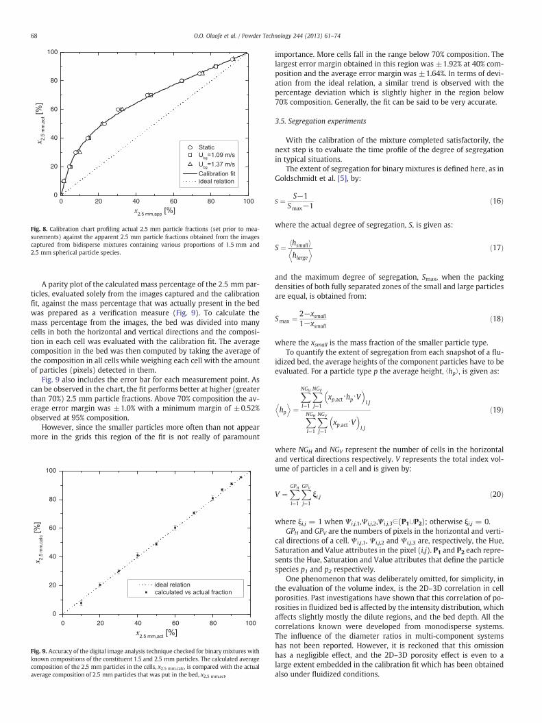
Once again, to demonstrate the calibration technique, the proce-dure and results for a bidisperse mixture of particles containing vari-ous compositions of the 1.5 mm and 2.5 mm species are presented. Inthe calibration conducted by Goldschmidt et al. [5], a bed with aknown composition was first fluidized at a velocity well above thatrequired from incipient fluidization, to thoroughly mix the particles,before the flow was stopped abruptly. The image of the bed is thentaken and analyzed for the calibration. In this work, in addition tostatic bed measurements, ‘in-situ’ calibration using images capturedin fluidized states were conducted. This was possible because evenat relatively large particle velocities the enhanced capacity of theimage capturing apparatus deployed in this work eliminates motion-blur effects.
Fig. 8 compares the calibration profile of the static measurements(taken after vigorous fluidization) with the profiles for measurementstaken during fluidization at 1.09 m/s and 1.37 m/s. These velocitiesare 1.2 and 1.5 times the incipient velocity, Umf, of a mixture containing50% 2.5 mm particles.
For the ‘in-situ’ calibration measurements, the apparent segregation(using apparent compositions) in each snapshot was evaluated andonly images in which the segregation was less than 10% were consid-ered. As a matter of fact, this criterion was necessary only for the1.09 m/s fluidization experiments because all the images captured dur-ing the 1.37 m/s experiments fell below the 10% segregation limit. Thesimilarity of the 3 sets ofmeasurements in Fig. 8 implies that the calibra-tion could be more quickly and easily done at an appropriate fluidizedstate because it excludes the time-consuming and less-convenientstop-start sequence involved in the static measurements.
Generally, for a bidisperse mixture, the calibration profile of thelarger specie can be represented by:
xp;act ¼ 1−að Þxp;app þ a 1−ebxcp;app
� �ð15Þ
where: xp,act is the actual fractional composition of particle type p inthe mixture, xp,app is the apparent fractional composition (in the bedsnaphots) of the particle type p in the mixture and a, b and c are thefit parameters.
Fig. 7. Bubble detection in a fluidized bed containing 50% 1.5 mm particles (green) and 50% 2.5 mm particles (blue) at a fluidization velocity of 1.09 m/s. (a.) Original, cropped snap-shot. (b.) Grayscale representation. (c.) Edges enhanced. (d.) Smearing with coarse filter. (e.) Bubbles identified. (f.) Bubbles subtracted and particles identified.
67O.O. Olaofe et al. / Powder Technology 244 (2013) 61–74
Typical values for the fit parameters are a = 0.45, b = −5.97,c = 0.8 (for the trend line in Fig. 8). The parameter a represents thelinear component of the fit relation and it corresponds to the intersec-tion of the tangent drawn at x2.5 mm,app = 100% (monodisperse bedwith 2.5 mm particles only) with the vertical axis at x2.5 mm,app =0%. Note that the fit parameters are unique to each specie pair. Thecalibration profiles change with particle sizes and colors, because ofslight differences (even as low as 4%) in densities, and the susceptibil-ity of the particles to static effects.
Furthermore, ordinarily, the calibration profiles would be expectedto exhibit a high degree of symmetry about the axis orthogonal to theideal relation at the middle of the chart but this is not the case. The de-viation from the ideal relation is found to be more pronounced whenthe larger 2.5 mm particles are present at relatively low volumetricfraction in the bed. This behavior is somewhat analogous to the trendseen in the packing fractions of FCC-ordered binary mixtures wherethe deviation from the monodisperse packing fraction is more whenthe larger particle is less in proportion [14].
Fig. 8. Calibration chart profiling actual 2.5 mm particle fractions (set prior to mea-surements) against the apparent 2.5 mm particle fractions obtained from the imagescaptured from bidisperse mixtures containing various proportions of 1.5 mm and2.5 mm spherical particle species.
A parity plot of the calculated mass percentage of the 2.5 mm par-ticles, evaluated solely from the images captured and the calibrationfit, against the mass percentage that was actually present in the bedwas prepared as a verification measure (Fig. 9). To calculate themass percentage from the images, the bed was divided into manycells in both the horizontal and vertical directions and the composi-tion in each cell was evaluated with the calibration fit. The averagecomposition in the bed was then computed by taking the average ofthe composition in all cells while weighing each cell with the amountof particles (pixels) detected in them.
Fig. 9 also includes the error bar for each measurement point. Ascan be observed in the chart, the fit performs better at higher (greaterthan 70%) 2.5 mm particle fractions. Above 70% composition the av-erage error margin was ±1.0% with a minimum margin of ±0.52%observed at 95% composition.
However, since the smaller particles more often than not appearmore in the grids this region of the fit is not really of paramount
100
80
60
40
20
0
0 20 40 60 80 100
Fig. 9. Accuracy of the digital image analysis technique checked for binary mixtures withknown compositions of the constituent 1.5 and 2.5 mm particles. The calculated averagecomposition of the 2.5 mm particles in the cells, x2.5 mm,calc, is compared with the actualaverage composition of 2.5 mm particles that was put in the bed, x2.5 mm,act.
importance. More cells fall in the range below 70% composition. Thelargest error margin obtained in this region was ±1.92% at 40% com-position and the average error margin was ±1.64%. In terms of devi-ation from the ideal relation, a similar trend is observed with thepercentage deviation which is slightly higher in the region below70% composition. Generally, the fit can be said to be very accurate.
3.5. Segregation experiments
With the calibration of the mixture completed satisfactorily, thenext step is to evaluate the time profile of the degree of segregationin typical situations.
The extent of segregation for binary mixtures is defined here, as inGoldschmidt et al. [5], by:
s ¼ S−1Smax−1
ð16Þ
where the actual degree of segregation, S, is given as:
S ¼ hsmallh ihlarge
D E ð17Þ
and the maximum degree of segregation, Smax, when the packingdensities of both fully separated zones of the small and large particlesare equal, is obtained from:
Smax ¼ 2−xsmall
1−xsmallð18Þ
where the xsmall is the mass fraction of the smaller particle type.To quantify the extent of segregation from each snapshot of a flu-
idized bed, the average heights of the component particles have to beevaluated. For a particle type p the average height, ⟨hp⟩, is given as:
hpD E
¼
XNGH
I¼1
XNGV
J¼1
xp;act⋅hp⋅V� �
I;J
XNGH
I¼1
XNGV
J¼1
xp;act⋅V� �
I;J
ð19Þ
where NGH and NGV represent the number of cells in the horizontaland vertical directions respectively. V represents the total index vol-ume of particles in a cell and is given by:
V ¼XGPH
i¼1
XGPV
j¼1
ξi;j ð20Þ
where ξi,j = 1 when Ψi,j,1,Ψi,j,2,Ψi,j,3∈(P1∪P2); otherwise ξi,j = 0.GPH and GPV are the numbers of pixels in the horizontal and verti-
cal directions of a cell. Ψi,j,1, Ψi,j,2 and Ψi,j,3 are, respectively, the Hue,Saturation and Value attributes in the pixel (i,j). P1 and P2 each repre-sents the Hue, Saturation and Value attributes that define the particlespecies p1 and p2 respectively.
One phenomenon that was deliberately omitted, for simplicity, inthe evaluation of the volume index, is the 2D–3D correlation in cellporosities. Past investigations have shown that this correlation of po-rosities in fluidized bed is affected by the intensity distribution, whichaffects slightly mostly the dilute regions, and the bed depth. All thecorrelations known were developed from monodisperse systems.The influence of the diameter ratios in multi-component systemshas not been reported. However, it is reckoned that this omissionhas a negligible effect, and the 2D–3D porosity effect is even to alarge extent embedded in the calibration fit which has been obtainedalso under fluidized conditions.
69O.O. Olaofe et al. / Powder Technology 244 (2013) 61–74
The xp,act in Eq. (19) is calculated for each cell from the calibrationfit in Eq. (15) by using the apparent fraction, xp,app, computed for eachcell. The apparent fraction for a particle type P1 is given by:
xp1 ;app ¼
XGPH
i¼1
XGPV
j¼1
ζ i;j
XGPHi¼1
XGPV
j¼1
ξi;j
ð21Þ
where ζi,j = 1 when Ψi,j,1,Ψi,j,2∈P1; otherwise ζi,j = 0.Similar relations can be written for systems with arbitrary number
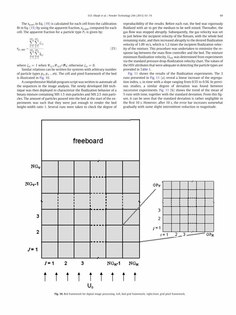
of particle types p2, p3 …etc. The cell and pixel framework of the bedis illustrated in Fig. 10.
A comprehensiveMatlab program scriptwaswritten to automate allthe sequences in the image analysis. The newly developed DIA tech-nique was then deployed to characterize the fluidization behavior of abinary mixture containing 50% 1.5 mmparticles and 50% 2.5 mmparti-cles. The amount of particles poured into the bed at the start of the ex-periments was such that they were just enough to render the bedheight-width ratio 1. Several runs were taken to check the degree of
Fig. 10. Bed framework for digital image processing. Left, b
reproducibility of the results. Before each run, the bed was vigorouslyfluidized with air to get the medium to be well mixed. Thereafter, thegas flow was stopped abruptly. Subsequently, the gas velocity was setto just below the incipient velocity of the flotsam, with the whole bedremaining static, and then increased abruptly to the desired fluidizationvelocity of 1.09 m/s, which is 1.2 times the incipient fluidization veloc-ity of the mixture. This procedure was undertaken to minimize the re-sponse lag between the mass flow controller and the bed. The mixtureminimum fluidization velocity, Umf, was determined from experimentsvia the standard pressure drop-fluidization velocity chart. The values oftheHSV attributes thatwere adequate in detecting the particle types areprovided in Table 1.
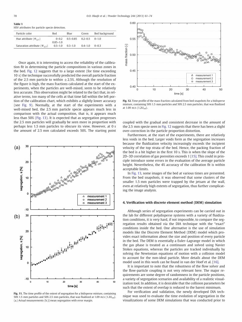
Fig. 11 shows the results of the fluidization experiments. The 3runs presented in Fig. 11 (a) reveal a linear increase of the segrega-tion index, s, in time with a slope ranging from 0.55 to 0.56. In previ-ous studies, a similar degree of deviation was found betweensuccessive experiments. Fig. 11 (b) shows the trend of the mean of5 runs with time, together with the standard deviation. From this fig-ure, it can be seen that the standard deviation is rather negligible inthe first 10 s. However, after 10 s, the error bar increases somewhatgradually with some slight intermittent reduction in magnitude.
ed grid framework; right/inset, grid pixel framework.
Table 1HSV attributes for particle specie detection.
Fig. 12. Time profile of the mass fraction calculated from bed snapshots for a bidispersemixture, containing 50% 1.5 mm particles and 50% 2.5 mm particles, that was fluidizedat 1.09 m/s (1.2Umf).
Once again, it is interesting to access the reliability of the calibra-tion fit in determining the particle compositions in various zones inthe bed. Fig. 12 suggests that to a large extent (for time exceeding10 s) the technique successfully predicted the overall particle fractionof the 2.5 mm particle to within ±2.5%. Although the resolution ofthe figure is high, the mass fractions calculated at the start of the ex-periments, when the particles are well-mixed, seem to be relativelyless accurate. This observation might be related to the fact that, in rel-ative terms, too many of the cells at that time fall within the left por-tion of the calibration chart, which exhibits a slightly lower accuracy(see Fig. 9). Normally, at the start of the experiments with awell-mixed bed, the 2.5 mm particle specie appears much less incomparison with the actual composition, that is, it appears muchless than 50% (Fig. 13). It is expected that as segregation progressesthe 2.5 mm particles will gradually be seen more in proportion withperhaps less 1.5 mm particles to obscure its view. However, at 0 sthe amount of 2.5 mm calculated exceeds 50%. The starting point
Fig. 11. The time profile of the extent of segregation for a bidisperse mixture, containing50% 1.5 mm particles and 50% 2.5 mm particles, that was fluidized at 1.09 m/s (1.2Umf).(a.) Actual measurements (b.)] mean segregation with error margin.
coupled with the gradual and consistent decrease in the amount ofthe 2.5 mm specie seen in Fig. 12 suggests that there has been a slightover-correction in the particle proportion distortion.
Furthermore, at the start of the experiments, there are relativelyless voids in the bed. Larger voids form as the segregation increasesbecause the fluidization velocity increasingly exceeds the incipientvelocity of the top strata of the bed. Hence, the packing fraction ofthe bed is a bit higher in the first 10 s. This is when the slope of the2D–3D correlation of gas porosities exceeds 1 [15]. This could in prin-ciple introduce some errors in the evaluation of the average particleheight. Nevertheless, the 4% accuracy of the calibration fit is withinacceptable limits.
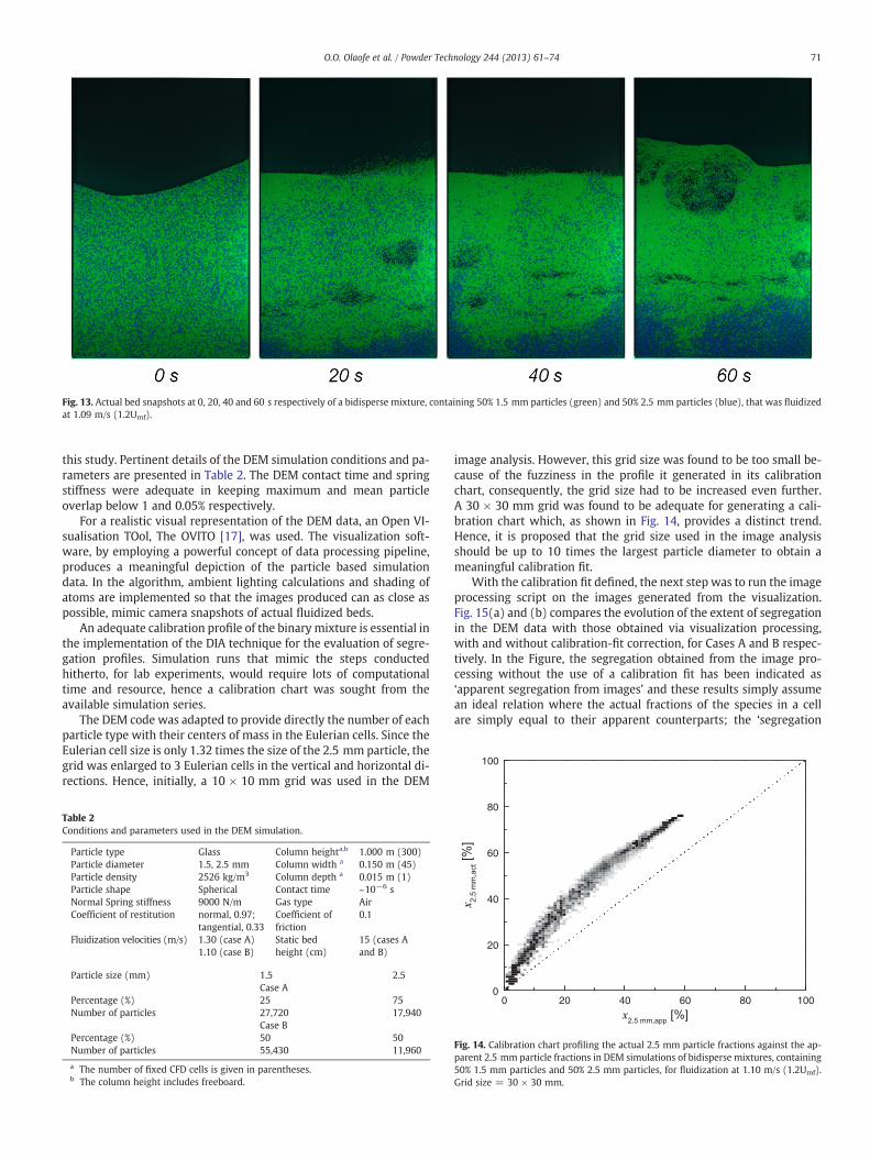
In Fig. 13, some images of the bed at various times are presented.From the bed snapshots, it was observed that some clusters of thesmaller 1.5 mm particles were trapped by the jetsam at the wall,even at relatively high extents of segregation, thus further complicat-ing the image analysis.
4. Verification with discrete element method (DEM) simulation
Although series of segregation experiments can be carried out inthe lab for different polydisperse systems with a variety of fluidiza-tion conditions, it is very hard, if not impossible, to compare the seg-regation results obtained via the DIA technique with the “exact”conditions inside the bed. One alternative is the use of simulationmodels like the Discrete Element Method (DEM) model which pro-vides exact information about the size and position of every particlein the bed. The DEM is essentially a Euler–Lagrange model in whichthe gas phase is treated as a continuum and solved using NavierStokes equations, whereas the particles are tracked individually bysolving the Newtonian equations of motion with a collision modelto account for the non-ideal particle. More details about the DEMmodel used in this work can be found in van der Hoef et al. [16].
It is important to note that the robustness of the flow solver andthe flow-particle coupling is not very relevant here. The major re-quirements are some degree of randomness in the particle positions,a variety of segregation scenarios and availability of a realistic visual-ization tool. In addition, it is desirable that the collision parameters besuch that the extent of overlap is reduced to the barest minimum.
For verification and validation, the newly developed DIA tech-nique was used to evaluate the time evolution of segregation in thevisualizations of some DEM simulations that was conducted prior to
Fig. 13. Actual bed snapshots at 0, 20, 40 and 60 s respectively of a bidisperse mixture, containing 50% 1.5 mm particles (green) and 50% 2.5 mm particles (blue), that was fluidizedat 1.09 m/s (1.2Umf).
100
71O.O. Olaofe et al. / Powder Technology 244 (2013) 61–74
this study. Pertinent details of the DEM simulation conditions and pa-rameters are presented in Table 2. The DEM contact time and springstiffness were adequate in keeping maximum and mean particleoverlap below 1 and 0.05% respectively.
For a realistic visual representation of the DEM data, an Open VI-sualisation TOol, The OVITO [17], was used. The visualization soft-ware, by employing a powerful concept of data processing pipeline,produces a meaningful depiction of the particle based simulationdata. In the algorithm, ambient lighting calculations and shading ofatoms are implemented so that the images produced can as close aspossible, mimic camera snapshots of actual fluidized beds.
An adequate calibration profile of the binary mixture is essential inthe implementation of the DIA technique for the evaluation of segre-gation profiles. Simulation runs that mimic the steps conductedhitherto, for lab experiments, would require lots of computationaltime and resource, hence a calibration chart was sought from theavailable simulation series.
The DEM code was adapted to provide directly the number of eachparticle type with their centers of mass in the Eulerian cells. Since theEulerian cell size is only 1.32 times the size of the 2.5 mm particle, thegrid was enlarged to 3 Eulerian cells in the vertical and horizontal di-rections. Hence, initially, a 10 × 10 mm grid was used in the DEM
Table 2Conditions and parameters used in the DEM simulation.
Particle type Glass Column heighta,b 1.000 m (300)Particle diameter 1.5, 2.5 mm Column width a 0.150 m (45)Particle density 2526 kg/m3 Column depth a 0.015 m (1)Particle shape Spherical Contact time ~10−6 sNormal Spring stiffness 9000 N/m Gas type AirCoefficient of restitution normal, 0.97;
tangential, 0.33Coefficient offriction
0.1
Fluidization velocities (m/s) 1.30 (case A)1.10 (case B)
Static bedheight (cm)
15 (cases Aand B)
Particle size (mm) 1.5 2.5Case A
Percentage (%) 25 75Number of particles 27,720 17,940
Case BPercentage (%) 50 50Number of particles 55,430 11,960
a The number of fixed CFD cells is given in parentheses.b The column height includes freeboard.
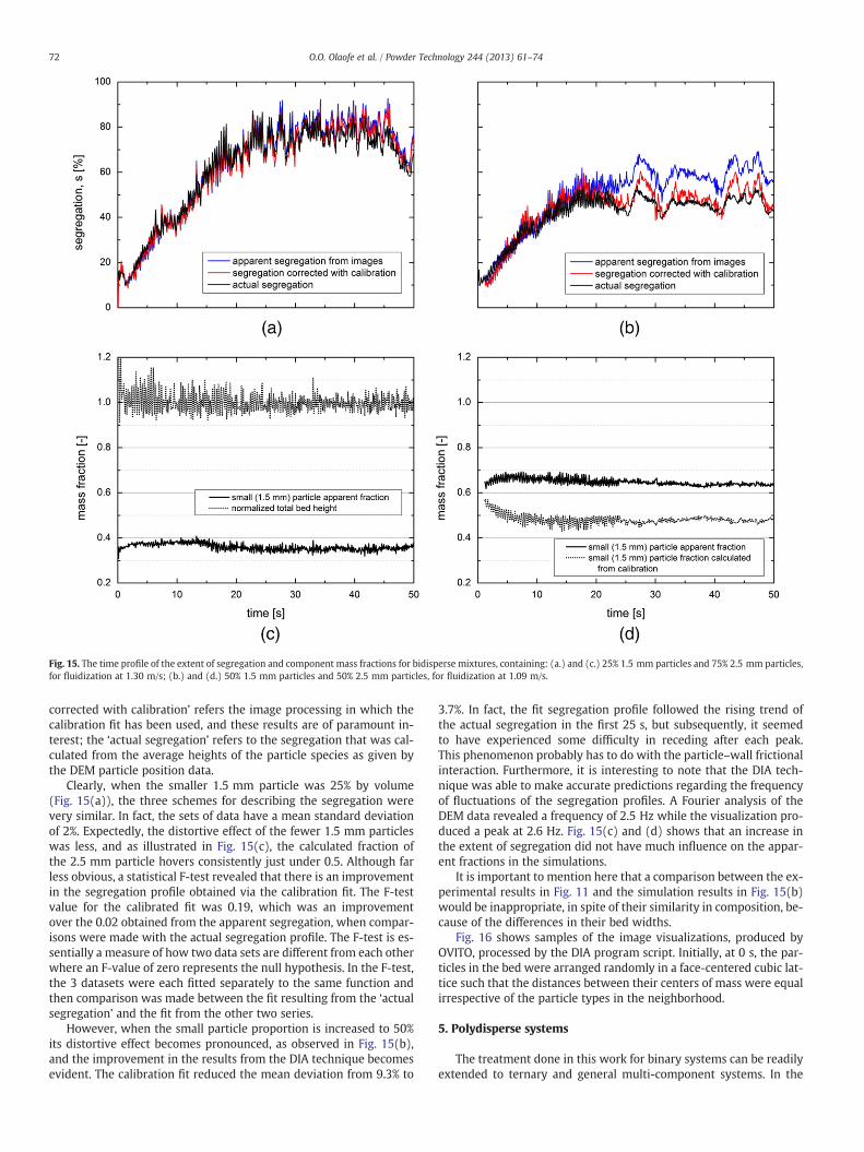
image analysis. However, this grid size was found to be too small be-cause of the fuzziness in the profile it generated in its calibrationchart, consequently, the grid size had to be increased even further.A 30 × 30 mm grid was found to be adequate for generating a cali-bration chart which, as shown in Fig. 14, provides a distinct trend.Hence, it is proposed that the grid size used in the image analysisshould be up to 10 times the largest particle diameter to obtain ameaningful calibration fit.
With the calibration fit defined, the next step was to run the imageprocessing script on the images generated from the visualization.Fig. 15(a) and (b) compares the evolution of the extent of segregationin the DEM data with those obtained via visualization processing,with and without calibration-fit correction, for Cases A and B respec-tively. In the Figure, the segregation obtained from the image pro-cessing without the use of a calibration fit has been indicated as‘apparent segregation from images’ and these results simply assumean ideal relation where the actual fractions of the species in a cellare simply equal to their apparent counterparts; the ‘segregation
80
60
40
20
00 20 40 60 80 100
Fig. 14. Calibration chart profiling the actual 2.5 mm particle fractions against the ap-parent 2.5 mm particle fractions in DEM simulations of bidisperse mixtures, containing50% 1.5 mm particles and 50% 2.5 mm particles, for fluidization at 1.10 m/s (1.2Umf).Grid size = 30 × 30 mm.
Fig. 15. The time profile of the extent of segregation and component mass fractions for bidisperse mixtures, containing: (a.) and (c.) 25% 1.5 mm particles and 75% 2.5 mm particles,for fluidization at 1.30 m/s; (b.) and (d.) 50% 1.5 mm particles and 50% 2.5 mm particles, for fluidization at 1.09 m/s.
corrected with calibration’ refers the image processing in which thecalibration fit has been used, and these results are of paramount in-terest; the ‘actual segregation’ refers to the segregation that was cal-culated from the average heights of the particle species as given bythe DEM particle position data.
Clearly, when the smaller 1.5 mm particle was 25% by volume(Fig. 15(a)), the three schemes for describing the segregation werevery similar. In fact, the sets of data have a mean standard deviationof 2%. Expectedly, the distortive effect of the fewer 1.5 mm particleswas less, and as illustrated in Fig. 15(c), the calculated fraction ofthe 2.5 mm particle hovers consistently just under 0.5. Although farless obvious, a statistical F-test revealed that there is an improvementin the segregation profile obtained via the calibration fit. The F-testvalue for the calibrated fit was 0.19, which was an improvementover the 0.02 obtained from the apparent segregation, when compar-isons were made with the actual segregation profile. The F-test is es-sentially a measure of how two data sets are different from each otherwhere an F-value of zero represents the null hypothesis. In the F-test,the 3 datasets were each fitted separately to the same function andthen comparison was made between the fit resulting from the ‘actualsegregation’ and the fit from the other two series.
However, when the small particle proportion is increased to 50%its distortive effect becomes pronounced, as observed in Fig. 15(b),and the improvement in the results from the DIA technique becomesevident. The calibration fit reduced the mean deviation from 9.3% to
3.7%. In fact, the fit segregation profile followed the rising trend ofthe actual segregation in the first 25 s, but subsequently, it seemedto have experienced some difficulty in receding after each peak.This phenomenon probably has to do with the particle–wall frictionalinteraction. Furthermore, it is interesting to note that the DIA tech-nique was able to make accurate predictions regarding the frequencyof fluctuations of the segregation profiles. A Fourier analysis of theDEM data revealed a frequency of 2.5 Hz while the visualization pro-duced a peak at 2.6 Hz. Fig. 15(c) and (d) shows that an increase inthe extent of segregation did not have much influence on the appar-ent fractions in the simulations.
It is important to mention here that a comparison between the ex-perimental results in Fig. 11 and the simulation results in Fig. 15(b)would be inappropriate, in spite of their similarity in composition, be-cause of the differences in their bed widths.
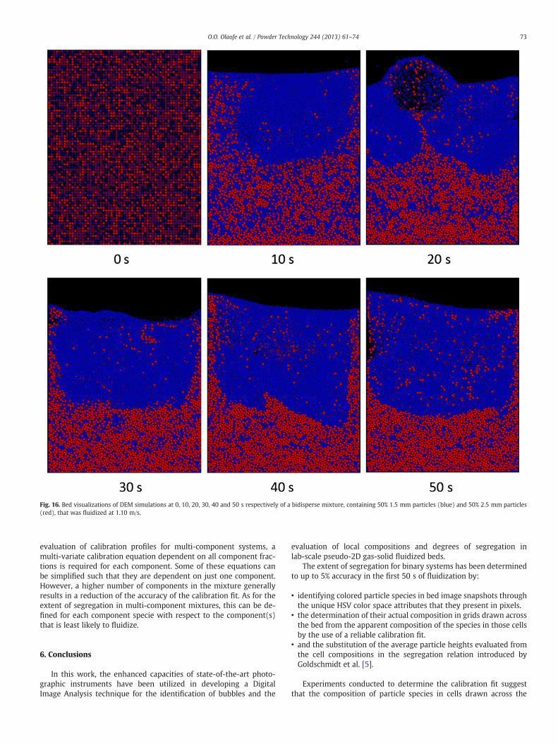
Fig. 16 shows samples of the image visualizations, produced byOVITO, processed by the DIA program script. Initially, at 0 s, the par-ticles in the bed were arranged randomly in a face-centered cubic lat-tice such that the distances between their centers of mass were equalirrespective of the particle types in the neighborhood.
5. Polydisperse systems
The treatment done in this work for binary systems can be readilyextended to ternary and general multi-component systems. In the
Fig. 16. Bed visualizations of DEM simulations at 0, 10, 20, 30, 40 and 50 s respectively of a bidisperse mixture, containing 50% 1.5 mm particles (blue) and 50% 2.5 mm particles(red), that was fluidized at 1.10 m/s.
73O.O. Olaofe et al. / Powder Technology 244 (2013) 61–74
evaluation of calibration profiles for multi-component systems, amulti-variate calibration equation dependent on all component frac-tions is required for each component. Some of these equations canbe simplified such that they are dependent on just one component.However, a higher number of components in the mixture generallyresults in a reduction of the accuracy of the calibration fit. As for theextent of segregation in multi-component mixtures, this can be de-fined for each component specie with respect to the component(s)that is least likely to fluidize.
6. Conclusions
In this work, the enhanced capacities of state-of-the-art photo-graphic instruments have been utilized in developing a DigitalImage Analysis technique for the identification of bubbles and the
evaluation of local compositions and degrees of segregation inlab-scale pseudo-2D gas-solid fluidized beds.
The extent of segregation for binary systems has been determinedto up to 5% accuracy in the first 50 s of fluidization by:
• identifying colored particle species in bed image snapshots throughthe unique HSV color space attributes that they present in pixels.
• the determination of their actual composition in grids drawn acrossthe bed from the apparent composition of the species in those cellsby the use of a reliable calibration fit.
• and the substitution of the average particle heights evaluated fromthe cell compositions in the segregation relation introduced byGoldschmidt et al. [5].
Experiments conducted to determine the calibration fit suggestthat the composition of particle species in cells drawn across the
bed can be determined reliably when the cell size is at least 10 timesthe diameter of the largest particle in the system.
The capability of the technique was demonstrated in the analysesof fluidized bed simulation results. In those analyses, the extents ofsegregation in snapshots of the DEM simulations were found to bein good agreement with exact values calculated from individual par-ticle positions in the DEM. The technique was also found to be sensi-tive enough to detect the frequency of fluctuations in the segregationprofile. The DEM probe seems to suggest that, for some binary mix-tures of certain diameter ratios, the time evolution of segregationcould be evaluated quite accurately, without recourse to the tediouscalibration procedure, when the smaller specie is present in a muchsmaller overall proportion.
Furthermore, the newly developed image analysis technique per-mits the simultaneous evaluation of bed height, and bubble size andposition by making use of robust in-built algorithms in Matlab.
We will use this DIA technique to examine other systems ofbidisperse and ternary mixtures in future work.
Notation
a fit parameterb fit parameterB(λ) sensitivity function for blue sensorc fit parameterG(λ) sensitivity function for green sensorGPH number of pixels in the horizontal direction of a cellGPV number of pixels in the vertical direction of a cell⟨hp⟩ average height of component particles of type p, mH Huei, I column indexj, J row indexΜ integration boundaries corresponding to the visible part of
the light spectrumNGH number of cells in the horizontal directionNGV number of cells in the vertical directionp particle typeR(λ) sensitivity function for red sensors extent of segregationS Saturation, or actual degree of segregationSmax maximum degree of segregationS(λ) visible part of the light spectrumUmf minimum fluidization velocity, m/sV Value, or the total index volume of particles in a cell
(Eqs. (19) and (20))xp,act actual fractional composition of particle type p in the mix-
ture, dimensionlessxp,app apparent fractional composition (in the bed snaphots) of
the particle type p in the mixture, dimensionlessxsmall mass fraction of the smaller particle type, dimensionless
Symbolλ wavelength of signal, nmΨi,j,1 Hue attribute in pixel (i,j)
Ψi,j,2 Saturation attribute in pixel (i,j)Ψi,j,3 Value attribute in pixel (i,j)
Acknowledgments
The authorswish to thank TheNetherlandsOrganization for ScientificResearch (NWO) for the financial support of this work.
References
[1] A. Busciglio, G. Vella, G. Micale, L. Rizzuti, Analysis of the bubbling behaviour of2D gas solid fluidized beds: Part I. Digital image analysis technique, ChemicalEngineering Journal 140 (1–3) (July 1 2008) 398–413.
[2] G.R. Caicedo, J.J.P. Marqués, M.G. Ruı́z, J.G. Soler, A study on the behaviour of bubblesof a 2D gas–solid fluidized bed using digital image analysis, Chemical Engineeringand Processing: Process Intensification 42 (1) (January 2003) 9–14.
[3] K.S. Lim, P.K. Agarwal, Conversion of pierced lengths measured at a probe to bub-ble size measures: an assessment of the geometrical probability approach andbubble shape models, Powder Technology 63 (3) (December 1990) 205–219.
[4] A.S. Hull, Z. Chen, J.W. Fritz, P.K. Agarwal, Influence of horizontal tube bankson the behavior of bubbling fluidized beds: 1. Bubble hydrodynamics, PowderTechnology 103 (3) (July 26 1999) 230–242.
[5] M.J.V. Goldschmidt, J.M. Link, S. Mellema, J.A.M. Kuipers, Digital image analysismeasurements of bed expansion and segregation dynamics in densegas-fluidised beds, Powder Technology 138 (2–3) (December 10 2003) 135–159.
[6] L. Shen, F. Johnsson, B. Leckner, Digital image analysis of hydrodynamics two-dimensional bubbling fluidized beds, Chemical Engineering Science 59 (13) (July2004) 2607–2617.
[7] G.A. Bokkers, M. van Sint Annaland, J.A.M. Kuipers, Mixing and segregation in abidisperse gas–solid fluidised bed: a numerical and experimental study, PowderTechnology 140 (3) (February 25 2004) 176–186.
[8] W. Cheng, Y. Murai, T. Sasaki, F. Yamamoto, Bubble velocity measurement with arecursive cross correlation PIV technique, Flow Measurement and Instrumenta-tion 16 (1) (March 2005) 35–46.
[9] C. Zhu, R.N. Dave, R. Pfeffer, Gas fluidization characteristics of nanoparticle ag-glomerates, AICHE Journal 51 (2) (2005) 426–439.
[10] X.S. Wang, V. Palero, J. Soria, M.J. Rhodes, Laser-based planar imaging of nano-particle fluidization: Part I—determination of aggregate size and shape, ChemicalEngineering Science 61 (16) (August 2006) 5476–5486.
[11] User Manual, AT-200GE Digital 3CCD Progressive Scan RGB Color Camera, January2011.
[12] M. Tkalcic, J.F. Tasic, Colour spaces: perceptual, historical and applicational back-ground, EUROCON 2003, computer as a tool, The IEEE Region 8 1 (2003) 304–308.
[13] A. Ford, A. Roberts, Colour space conversioins, Last accessed: December 4th, 2012Retrieved from http://www.poynton.com/PDFs/coloureq.pdf August 1998(b).
[14] H.J.H. Brouwers, Packing of crystalline structures of binary hard spheres: an analyt-ical approach and application to amorphization, Physical Review E — Statistical,Nonlinear, and Soft Matter Physics 76 (2007) 041304.
[15] J.F. de Jong, S.O. Odu, M.S. van Buijtenen, N.G. Deen, M. van Sint Annaland, J.A.M.Kuipers, Development and validation of a novel digital image analysis method forfluidized bed particle image velocimetry, Powder Technology 230 (November2012) 193–202.
[16] M.A. van der Hoef, M. Ye, M. van Sint Annaland, A.T. Andrews IV, S. Sundaresan,J.A.M. Kuipers, Multiscale modeling of gas-fluidized beds, Advances in ChemicalEngineering 31 (2006) 65–149.
[17] A. Stukowski, Visualization and analysis of atomistic simulation data with OVITO—the Open Visualization Tool, Modelling and Simulation in Materials Science andEngineering 18 (2010) 015012.