Improving Social Policy through Spatial Information: Application of Small Area Estimation and Spatial Microsimulation Methods in Geographical Targeting Noriel Christopher C. Tiglao, Dr. Eng. National College of Public Administration and Governance, University of the Philippines DDSS Conference, 7 July 2006 Heeze, The Netherlands
Transcript
Improving Social Policy through Spatial Information:Application of Small Area Estimation and Spatial Microsimulation Methods in Geographical Targeting
Noriel Christopher C. Tiglao, Dr. Eng.National College of Public Administration and Governance, University of the Philippines
DDSS Conference, 7 July 2006Heeze, The Netherlands
Framework for Generation of Spatial InformationConcluding Remarks
3
Introduction
Social policy is the study of social welfare, and its relationship to politics and societyPrincipal areas include health administration, social security, education, employment services; also includes social problems, such as crime, disability, unemployment, mental health, and old ageMajor goal of social policy in developing countries is poverty alleviation
4
Role of Spatial Information in Social Policy
Strong influence on economic and technical developmentExtending beyond the scope of central government to include local government and civil societyCritical in processes of consultation and consensus building among policymaking groups
5
Social Policy Administration
Debate between universalism and selectivity (targeting)
Universal policies can reach everyone on the same terms and this has been the argument for public services such as roads or parks, including education and health services.Targeted programs are often considered as being more efficient, that is, it takes less money to realize the benefits.
6
Targeting of Social Programs
Universal programs are too expensive for most developing countries, and even many industrial countries find the rising welfare costs dauntingThe only viable option, therefore, is to use some form of targeting
Requires a careful choice of the targeting criteria, the observable indicators that will determine eligibility, and the programs that be fit the specific conditions of the country or locality
7
Targeting Methods
Targeting by activity – e.g. health care, educationTargeting by indicator - alternatives to income, that are expected to be correlated with poverty, are used to identify the poorTargeting by location, where area of residence becomes the criteria for identifying the target groupTargeting by self-selection or self-targeting, where programs are designed to be attractive only to the poor, e.g. work-for-food programs
8
Geographical Targeting
The optimum solution in welfare programs, from a theoretical point of view, is to identify the target population and design the most effective program for this groupIn most cases, however, it is not possible to identify the target population since this requires information that is not observable and thus difficult to verify
9
Geographical Targeting
In poverty alleviation programs, the target population is the group of households with incomes below a certain minimum level necessary to provide basic needs. Household income is often difficult to observe, however, and efforts to assess its value and thus identify the target group may involve prohibitive costs
10
Geographical Targeting
These costs consist not only of direct administrative expenses for collecting the necessary information on income, but also of indirect costs due to incentives that the program may give individuals either to modify their behavior or to falsify information on their income in order to qualify for the program’s benefits
Ex. Poverty alleviation programs such as income transfers or food subsidies to the poor, for example, may provide incentives to work less, cut earnings, or underreport income in order to qualify
11
Small Area Estimation
Small area estimation has received a lot of attention in recent years due to growing demand for reliable small area estimatorsTraditional area-specific direct estimators do not provide adequate precision because sample sizes in small areas are seldom large enoughSample surveys are used to provide estimates not only for the total population but also for a variety of subpopulations (domains)
12
Small Area Estimation
“Direct” estimators, based only on the domain-specific sample data, are typically used to estimate parameters for large domainsBut sample sizes in small domains, particularly small geographic areas, are rarely large enough to provide direct estimates for specific small domains
13
Types of Small Area Estimation Models
i ~ IID N(0, b2)
~ known positive constants
~ IID N(0, e2)
i ~ IID N(0, b2)
• Unit-level Model (Battese et al., 1988)
i i i iy x z
i i i ijy x e
• Area-level Model (Fay and Herriot, 1979)
iz
ije
14
Building footprint and land use data in GIS
Small Area Estimation of Mean Household Incomes in Manila City
yij =x′ij β + uij
• Nested Error Linear Regression (EBLUP)
yij : mean household income for traffic zone j in city iυi : i-th city effecteij : randoms effect associated with zone j in city i
covariate used is average dwelling unit size
uij = υi + eij
15
City No. of zones
EBLUP Survey regression
Direct estimates
Manila 54 0.039 0.035 0.031
Pasay 11 0.069 0.031 0.029
Makati 18 0.060 0.162 0.242
Mandaluyong 8 0.070 0.185 0.304
San Juan 4 0.089 0.390 0.560
Quezon City 57 0.038 0.034 0.042
Caloocan 17 0.061 0.026 0.036
Valenzuela 9 0.072 0.034 0.028
Malabon 7 0.077 0.048 0.097
Navotas 5 0.082 0.032 0.560
Marikina 8 0.074 0.046 0.050
Pasig 11 0.069 0.054 0.051
Parañaque 15 0.063 0.130 0.122
Muntinlupa 7 0.077 0.215 0.141
Las Piñas 8 0.074 0.083 0.056
Standard error of estimates
16
Spatial Microsimulation
Developed by Guy Orcutt in 1957; ‘A new kind of socio-economic system’Directly concerned with microunits such as persons, households, or firmsModels lifecycle by the use of conditional probabilitiesOne major objective in spatial microsimulation is the estimation of microdata
17
Spatial Microsimulation (cont.)
Spatial microsimulation is increasingly applied in the quantitative analysis of economic and social policy problems (Clarke, 1996)
2. Probability of hhof give age, sex,and M being anowner-occupier
3. Random number(computer generated)
4. Tenure assignedto hh on basis of random sampling
5. Next hh (keeprepeating until a tenure type hasbeen allocated to
Age: 27Sex: maleM: married
0.7
0.542
owner-occupied
Age: 32Sex: maleM: married
0.7
0.823
rented
Age: 87Sex: femaleM: divorced
0.54
0.794
rented
Source: Clarke (1996)
Example of spatial microsimulation process
19
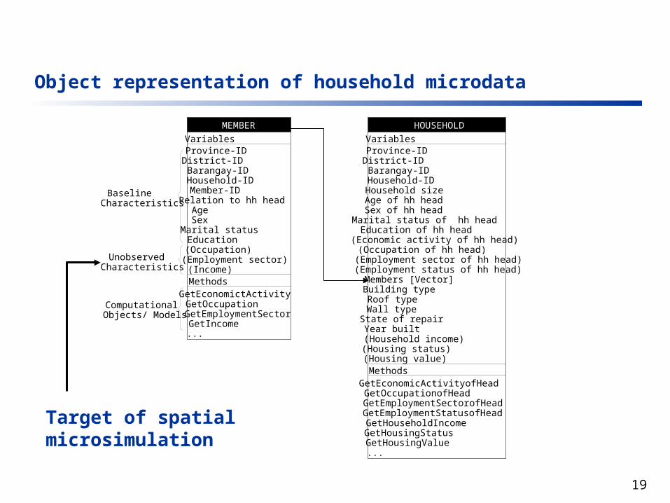
HOUSEHOLD
VariablesProvince-IDDistrict-IDBarangay-IDHousehold-IDHousehold sizeAge of hh headSex of hh headMarital status of hh headEducation of hh head(Economic activity of hh head)(Occupation of hh head)(Employment sector of hh head)(Employment status of hh head)Members [Vector]Building typeRoof typeWall typeState of repairYear built(Household income)(Housing status)(Housing value)MethodsGetEconomicActivityofHeadGetOccupationofHeadGetEmploymentSectorofHeadGetEmploymentStatusofHeadGetHouseholdIncomeGetHousingStatusGetHousingValue...
MEMBER
VariablesProvince-IDDistrict-IDBarangay-IDHousehold-IDMember-IDRelation to hh headAgeSexMarital statusEducation(Occupation)(Employment sector)(Income)MethodsGetEconomictActivityGetOccupationGetEmploymentSectorGetIncome...
BaselineCharacteristics
UnobservedCharacteristics
ComputationalObjects/ Models
Object representation of household microdata
Target of spatial microsimulation
20
HOUSEHOLD
VariablesProvince-IDDistrict-IDBarangay-IDHousehold-IDHousehold sizeAge of hh headSex of hh headMarital status of hh headEducation of hh head(Economic activity of hh head)(Occupation of hh head)(Employment sector of hh head)(Employment status of hh head)Members [Vector]Building typeRoof typeWall typeState of repairYear built(Household income)(Housing status)(Housing value)MethodsGetEconomicActivityofHeadGetOccupationofHeadGetEmploymentSectorofHeadGetEmploymentStatusofHeadGetHouseholdIncomeGetHousingStatusGetHousingValue...
Spatial attribute of household microdata
21
Spatial microsimulation of informal households in Manila City
• Manila City (54 traffic zones, 900 barangays, 1.59 million pop. in 1990, 308,874 households)
22
Available data sets
• Detailed household and housing characteristics
• No income/employment variable• Non-response on housing variables• All households in 1990 (1,567,665
households)
1990 Census of Population and Housing (CPH)
Barangay
Description/ CoverageData SetZone System
1996 MMUTIS Land Use GIS1997 Building Footprint Data
1996 Metro Manila Urban Transportation Integration Study (MMUTIS)
1997 Family Income and Expenditure Survey (FIES)
• Urban land use zoning map for entire Metro Manila
• Building footprints for most cities
GIS
• Selected household demographics• Member/ household income• 50,000 samples for Metro Manila
Traffic Zone
• Household demographics, some housing variables
• Detailed household incomes and expenditures
• 4,030 samples for Metro Manila
City
23
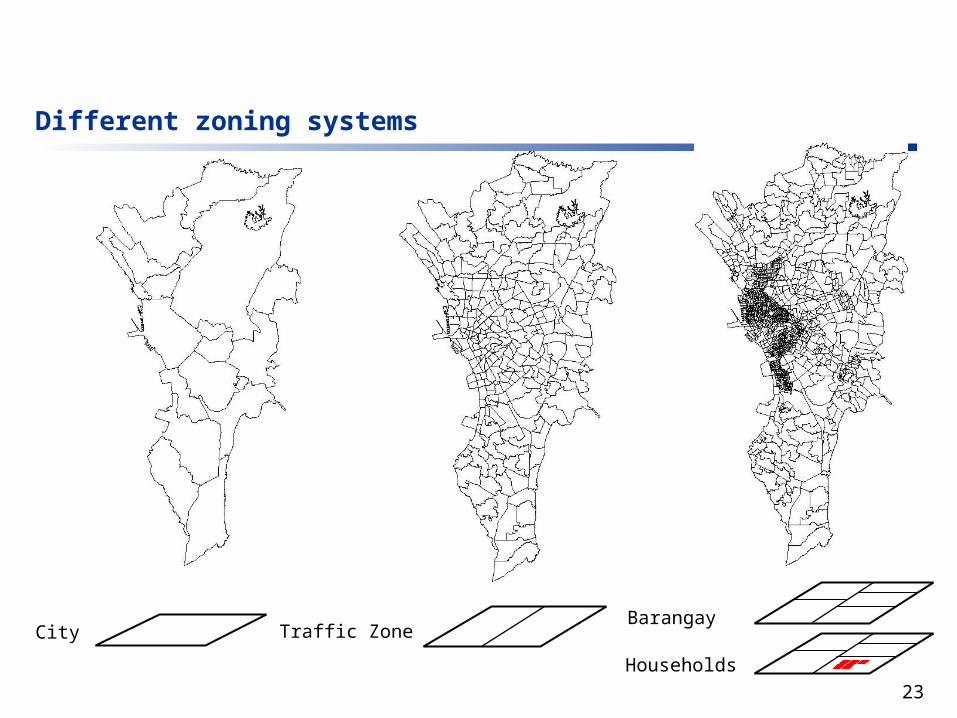
Different zoning systems
City Traffic ZoneBarangay
Households
24
Initialize base householdsusing 1990 CPH data
(age, sex, marital status,and education of household
head, household size)
Assign occupation ofhousehold head based
on Monte Carlo sampling
Assign employment sectorof household head basedon Monte Carlo sampling
Compute occupation probabilities from
Occupation Choice Model
Compute employmentprobabilities from
Employment Choice Model
Estimate household incomebased on characteristics
of household head
Compute employment status probabilities and
assign employment statusby Monte Carlo sampling
Compute bias-adjustedhousehold income function
based on employment status
Compute economic activityrate of household head
Estimate permanentIncome of household
Compute housing tenure status probabilities and
assign housing tenure statusby Monte Carlo sampling
Compute bias-adjustedhousing value functionbased on tenure status
Estimate housing tenureand housing value
Spatial microsimulationsystem for estimating household characteristics
25
Simulated mean household incomes
Low
Low
High
Middle
Low
High
26
Ground truths
Smokey Mountain
Port Area, Tondo
Pandacan
Punta
27
Simulated housing tenure
28
Simulated informal employment
29
Inequality measures
30
Estimation of mean household incomes
at the traffic zone level
Reliable estimates of mean household incomes
at traffic zone level
Estimation of household characteristics including
household income
VALIDATION
STATISTICAL SMALL AREA ESTIMATION
SPATIALMICROSIMULATION
Calculate mean household incomes at
traffic zone level
Survey data of household incomes
Framework for Generation of Spatial Information
31
Validation of Microsimulation ResultsEBLUP-DWELLING Benchmark
0
5000
10000
15000
20000
25000
30000
0 5000 10000 15000 20000 25000 30000
Estimated True Values
Sim
ula
ted
Va
lue
s
Framework for Generation of Spatial Information
Validation of spatial microsimulation output
32
Concluding Remarks
Small Area Estimation and Spatial Microsimulation methods can overcome data problems in ‘data-poor’environmentsResulting microdata enables analyst to make full use of existing but disparate data sets and produce reliable and spatially-disaggregate informationFurther research work should be pursued in developing the methods as practical tools for improving social policy