In-situ measurement of borehole thermal properties in Melbourne
Tshewang Lhendup, Lu Aye*, Robert James FullerRenewable Energy and Energy Efficiency Group, Department of Infrastructure Engineering, Melbourne School of Engineering, The University of Melbourne,Victoria 3010, Australia
h i g h l i g h t s
� In-situ thermal response of borehole heat exchangers in Melbourne were analysed.� Slope determination, two variable parameter fitting and the GPM model were applied.� Three thermal conductivity values obtained were applied in TRNSYS simulations.� The GPM model provides better agreement with measured temperatures from boreholes.
a r t i c l e i n f o
Article history:Received 12 March 2014Accepted 21 July 2014Available online 31 July 2014
The ability to quantify the ground thermal properties of a site is important for the appropriate sizing ofground heat exchangers. This paper presents the results of in-situ measurements of the thermal prop-erties of two 40 m deep borehole thermal storage systems in Melbourne. The measurements from thetests were analysed using three methods: conventional slope determination, two variable parameterfitting technique and using Geothermal Properties Measurement (GPM) model. The values of effectivethermal conductivities obtained from the three methods were applied in 12 TRNSYS simulations. Thevalue from the GPM model was found to give relatively less error when the measured and simulatedoutlet temperatures were compared.
The effective thermal conductivity of the soil and boreholethermal resistance are important parameters for sizing the bore-hole heat exchanger (BHE) of an inter-seasonal thermal storagesystem or a ground-coupled heat pump. These properties vary withthe type of soil, local soil moisture content and particle size andhence are site-specific. Moreover, soil type variation within aborehole depth may also exist. It is therefore necessary to deter-mine the thermal properties of the ground at each specific instal-lation site. The effective ground thermal conductivity and effectiveborehole thermal resistance can be determined either by referringto existing literature relevant to the type of soil, conducting heatprobe tests on soil samples or by performing an in-situ test [1e3].
For an estimation of the soil thermal conductivity based on theliterature, the task is to identify the type of soil and its moisturecontent and refer to the existing data. As the soil type may vary
8evier Ltd. All rights reserved.
along the length of the borehole, this estimate may not necessarilyrepresent the true value as the estimate is confined to only one typeof soil layer. The data on soil thermal conductivity is available for arange of soil types in the literature as shown in Table 1 [1,2,4e6].Similarly, the volumetric heat capacity of the soil is also determinedbased on the type of soil.
Another method to determine the soil thermal conductivity isby a heat probe test [7e9]. The test is performed on a soil sample ina laboratory [1]. In this method, constant heat is supplied to the soiland the corresponding change in soil temperature is observed overa given time period. Based on the temperature change of the soil,the thermal conductivity can be determined by a parametric esti-mation. Because only a small sample of soil is tested, the valueobtained may not be considered to be representative for the entiredepth of the borehole. Since the borehole may have different typesof soil along its length with different thermal properties, estimatesfrom this method may also not be representative of the entirelength of the borehole.
The third method of determining ground thermal properties isby an in-situ thermal response test (TRT) combined with a para-metric estimation algorithm [2,3,10,11]. This method is a mimic ofthe BHE system. It was first proposed byMogensen [12] and further
T. Lhendup et al. / Applied Thermal Engineering 73 (2014) 285e293286
studied and developed by Austin [3], Austin, Yavuzturk and Spitler[13] and Gehlin [14]. Since then several researchers [1,10,15e19]have used the TRT method to determine the BHE thermal con-ductivity based on the methodology described by the above au-thors. The principle of the TRT is based on constant heat injectionfrom a source for 50e60 h by using the BHE. Austin [3] found thatby conducting the test for a minimum of 50 h, the BHE thermalconductivity obtained would be within 2% of the value that wouldbe obtained had the test been conducted for a longer duration. Asthe performance of the system is not only affected by the soilthermal properties but also by the properties of the grout, U-tubepipe and heat transfer fluid, the thermal conductivity obtained bythis method is the effective thermal conductivity of the groundconsidering the BHE characteristics.
The value of measured effective thermal conductivity from theTRT is influenced by the duration of the test. The heat transferduring the initial few hours of the test is dominated by transienteffects. Therefore, it is recommended to disregard the measureddata during the initial 10e15 h [14]. This is mainly to avoid transienttemperature gradients and using data which is significantly influ-enced by the grout thermal properties. Austin [3] found that bestestimates were obtained when 12 h of initial datawere disregardedand Gehlin [20] suggests discarding 12e20 h initial data whenprocessing the experimental data. The number of hours to discarddepends onwhen the temperature reaches a steady state. A furtherstudy conducted by Yu et al. [21] found that after 35 h of testing, thevalue of measured effective thermal conductivity became relativelyconstant.
The inconsistency in the value of soil thermal conductivityresulting from the different methods was reported byWitte, Gelderand Spitler [1]. They compared the values of soil thermal parame-ters by several methods. The types of soil while drilling a 35 mborehole were identified. The borehole comprised of 11 differentsoil types. Based on these,Witte, Gelder and Spitler [1] obtained thesoil thermal conductivity for each layer from the literature. Theyestimated soil thermal conductivity for the borehole to vary from1.2 to 3.4 W m�1 K�1 with weighted average of 1.90 W m�1 K�1.Next they determined soil thermal conductivity by performing theheat probe test on nine samples from different layers of soil fromthe same borehole. Themeasured thermal conductivity varied from1.09 to 2.87Wm�1 K�1 with aweighted average of 2.09Wm�1 K�1.Finally, the effective soil thermal conductivity was determined byconducting an in-situ test on the same borehole. From the test theyestimated the average effective soil thermal conductivity to be2.10 W m�1 K�1. While these estimates show that the soil thermalconductivity obtained by the laboratory and in-situ test are almostequal, the results may have been different had the laboratory testbeen conducted on only one soil sample.
Similar results were obtained in another test conducted byWitte [5] in Netherlands. The researcher estimated soil thermalconductivity to be 1.83 W m�1 K�1 from the literature,2.10 W m�1 K�1 from a laboratory test and 2.13 from in-situ test. Inboth the studies, the authors observed that the average soil thermal
conductivity estimate based on reference tables to be the lowest,followed by the laboratory test and the in-situ test. These com-parisons suggest that the value obtained for the thermal conduc-tivity of the soil varies with the method used to determine it.Furthermore, the literature also suggests that the most commonand accepted method is the TRT. Since an estimation of effectivethermal conductivity of soil of the borehole on site is essential, theTRT method was used to determine the effective soil thermalconductivity and borehole effective thermal resistance of boreholesto be used for an inter-seasonal underground thermal storagesystemwhich is located at the Burnley campus of the University ofMelbourne. Thus, the aim of this paper is to determine the thermalconductivity and resistance of the boreholes used for inter-seasonalheat and coolth storage in Melbourne. The measurements from thetests were analysed using three methods: conventional slopedetermination, two variable parameter fitting technique and usingGeothermal Properties Measurement (GPM) model.
2. TRT set up
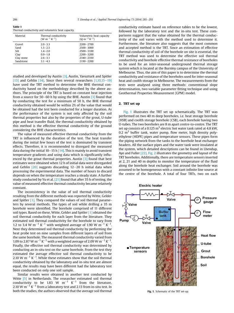
Fig. 1 illustrates the TRT set up schematically. The TRT wasperformed on two 40 m deep boreholes, i.e. heat storage borehole(HSB) and coolth storage borehole (CSB), each borehole having twoU-tubes. The two boreholes are 8 m apart centre-to-centre. The TRTset up consists of a 0.125 m3 electric hot water tank rated at 4.8 kW,0.2 m3 buffer tank, water pump, flow meter, high density poly-ethylene (HDPE) pipes and temperature sensors. These pipes formthe piping network from the tanks to the borehole heat exchangerheaders. All the surface pipes and the water tank were insulated atthe system, which detailed descriptions can be found in Lhendup,Aye and Fuller [22]. Fig. 2 illustrates the geometry and layout of theTRT boreholes. Additionally, there are temperature sensors insertedat 2, 21 and 40 m depths to monitor the temperature of the fluidalong the borehole heat exchanger. Soil around the borehole wasassumed to be homogeneous with a constant infinite line source atthe centre of the borehole. A total of four TRTs, two on each
Fig. 2. Layout and geometry of TRT boreholes.
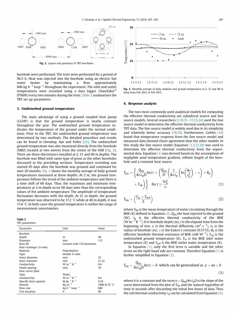
Fig. 3. Monthly average of daily ambient and ground temperature at 2, 21 and 40 mdeep from Feb 2012 to Feb 2013.
T. Lhendup et al. / Applied Thermal Engineering 73 (2014) 285e293 287
borehole were performed. The tests were performed for a period of96.5 h. Heat was injected into the borehole using an electric hotwater heater by maintaining a flow approximately840 kg h�1 loop�1 throughout the experiment. The inlet and outlettemperatures were recorded using a data logger (DataTaker®
DT600) every twominutes during the tests. Table 2 summarises theTRT set up parameters.
3. Undisturbed ground temperature
The main advantage of using a ground coupled heat pump(GCHP) is that the ground temperature is nearly constantthroughout the year. The undisturbed ground temperature in-dicates the temperature of the ground under the normal condi-tions. Prior to the TRT, the undisturbed ground temperature wasdetermined by two methods. The detailed procedure and resultscan be found in Lhendup, Aye and Fuller [22]. The undisturbedground temperature was also measured directly from the borehole(MB2) located at two metres from the centre of the HSB (Fig. 2).There are three thermistors installed at 2, 21 and 40 m depths. Theborehole was filled with same type of grout as the other boreholesdiscussed in the preceding sections. Temperature recording wasstarted 45 days after the borehole was grouted and continued fornext 20 months. Fig. 3 shows the monthly average of daily groundtemperatures measured at those depths. At 2 m, the ground tem-perature follows the trend of the ambient temperature and there isa time shift of 60 days. Thus, the maximum and minimum tem-peratures at 2 m depth occur 60 days later than the correspondingvalues of the ambient temperature. The amplitude of temperaturefluctuation decreases with the depth. At 21 m depth, the groundtemperature was observed to be 17.2 �C while at 40 m depth, it was17.4 �C. In both cases the ground temperature is within the range ofmeasurement uncertainties.
Table 2TRT parameters.
Parameter Unit Value
BoreholeDepth m 40Diameter mm 115Back fill Cement with 15% bentoniteHeat exchanger (U-tube)Material PolyethyleneType Double U-tubeOuter diameter mm 25Inner diameter mm 21.32Conductivity W m�1 K�1 0.4Shank spacing mm 70Heat carrier fluidType WaterConductivity W m�1 K�1 0.6Specific heat capacity kJ kg�1 K�1 4.18Density Kg m�3 1000 @ 25 �CFlow rate kg h�1 loop�1 840Test duration h 96
4. Response analysis
The two most-commonly used analytical models for computingthe effective thermal conductivity are cylindrical source and linesource models. Several researchers [1,10,15e17,23,24] used the linesource model to determine the effective thermal conductivity fromTRT data. The line source model is widely used due to its simplicityand relatively better accuracy [10,14]. Furthermore, Gehlin [14]found that temperature response from the line source model andmeasured data showed closer agreement than the other models. Inthis study the line source model (Equation (1)) [3,14] was used todetermine the effective thermal conductivity from the experi-mental data. Equation (1) was derived based on the assumptions ofnegligible axial temperature gradient, infinite length of the bore-hole and a constant heat source.
Tfm ¼(
Qinj
4plgDlnðtÞ þ
Qinj
D
1
4plg
ln
4ar2b
!� g
!þ Rb
!
þ Tug
!)for t� 5r2b
a(1)
Tfm ¼�Tin þ Tout
2
�(2)
where Tfm is themean temperature of water circulating through theBHE (K) defined in Equation (2), Qinj the heat injected to the ground(W), lg is the effective thermal conductivity of the BHE(Wm�1 K�1), D is borehole depth (m), t is the elapsed time from thebeginning of test, a is the thermal diffusivity (m2 s�1), rb is theradius of borehole (m), g is the Eulers's constant (0.5772), Rb is theeffective borehole thermal resistance of BHE (mK W�1), Tug is theundisturbed ground temperature (K), Tin is the BHE inlet watertemperature (K) and Tout is the BHE outlet water temperature (K).
In Equation (1), only the first term is variable and the otherterms on the right hand side are constant. Therefore Equation (1) isfurther simplified to Equation (3).
Tfm ¼ Qinj
4plgDlnðtÞ þ b which can be generalised as y ¼ axþ b
(3)
where b is a constant and the term a¼ Qinj/4plgD is the slope of thecurve determined from the plot of Tfm and the natural logarithm oftime in seconds after discarding the initial few hours of data. Thusthe soil thermal conductivity lg can be calculated fromEquation (4).
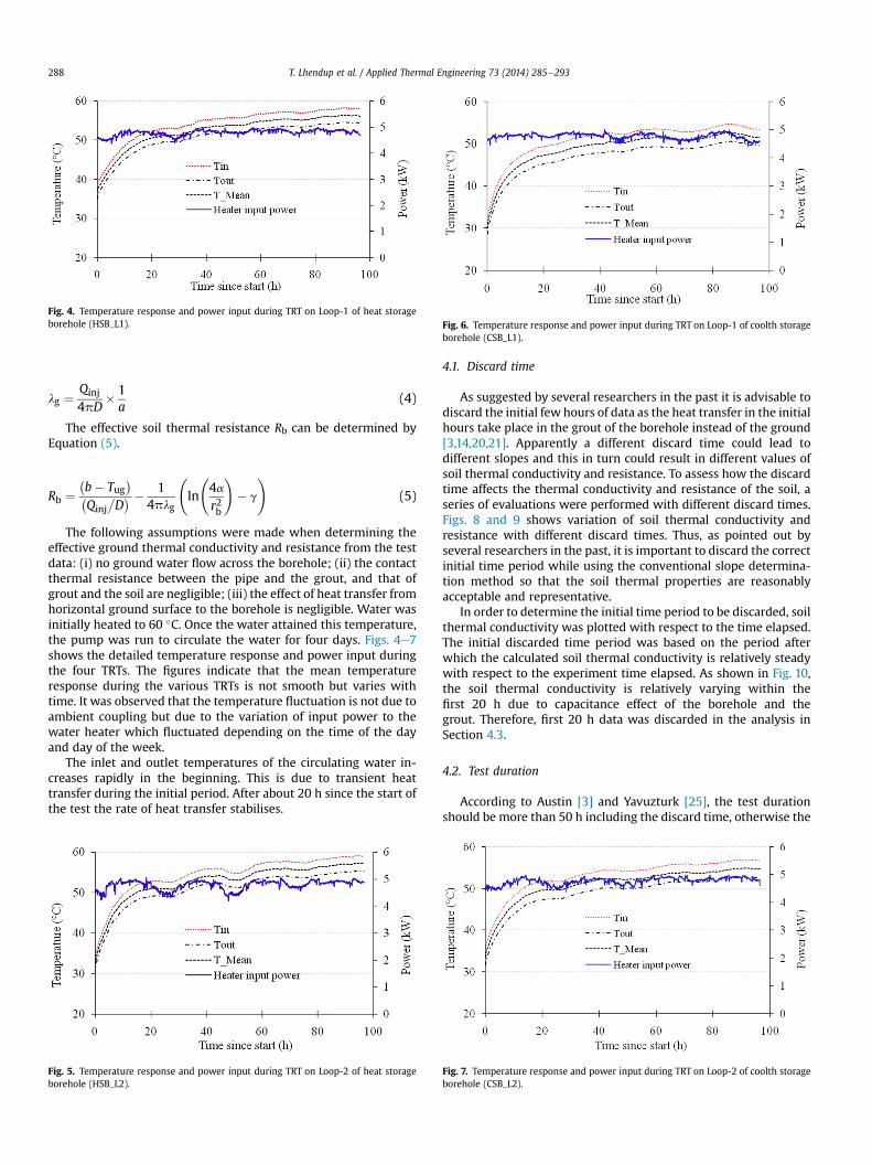
Fig. 4. Temperature response and power input during TRT on Loop-1 of heat storageborehole (HSB_L1). Fig. 6. Temperature response and power input during TRT on Loop-1 of coolth storage
borehole (CSB_L1).
T. Lhendup et al. / Applied Thermal Engineering 73 (2014) 285e293288
lg ¼ Qinj
4pD� 1
a(4)
The effective soil thermal resistance Rb can be determined byEquation (5).
Rb ¼�b� Tug
��Qinj
�D� � 1
4plg
ln
4ar2b
!� g
!(5)
The following assumptions were made when determining theeffective ground thermal conductivity and resistance from the testdata: (i) no ground water flow across the borehole; (ii) the contactthermal resistance between the pipe and the grout, and that ofgrout and the soil are negligible; (iii) the effect of heat transfer fromhorizontal ground surface to the borehole is negligible. Water wasinitially heated to 60 �C. Once the water attained this temperature,the pump was run to circulate the water for four days. Figs. 4e7shows the detailed temperature response and power input duringthe four TRTs. The figures indicate that the mean temperatureresponse during the various TRTs is not smooth but varies withtime. It was observed that the temperature fluctuation is not due toambient coupling but due to the variation of input power to thewater heater which fluctuated depending on the time of the dayand day of the week.
The inlet and outlet temperatures of the circulating water in-creases rapidly in the beginning. This is due to transient heattransfer during the initial period. After about 20 h since the start ofthe test the rate of heat transfer stabilises.
Fig. 5. Temperature response and power input during TRT on Loop-2 of heat storageborehole (HSB_L2).
4.1. Discard time
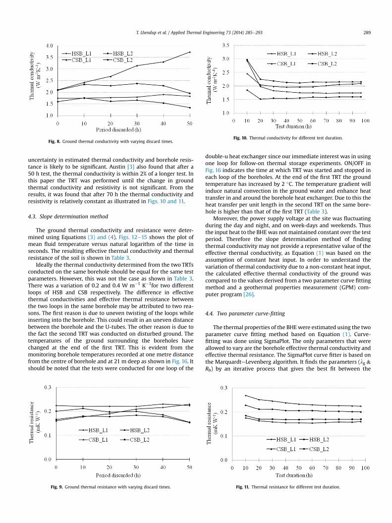
As suggested by several researchers in the past it is advisable todiscard the initial few hours of data as the heat transfer in the initialhours take place in the grout of the borehole instead of the ground[3,14,20,21]. Apparently a different discard time could lead todifferent slopes and this in turn could result in different values ofsoil thermal conductivity and resistance. To assess how the discardtime affects the thermal conductivity and resistance of the soil, aseries of evaluations were performed with different discard times.Figs. 8 and 9 shows variation of soil thermal conductivity andresistance with different discard times. Thus, as pointed out byseveral researchers in the past, it is important to discard the correctinitial time period while using the conventional slope determina-tion method so that the soil thermal properties are reasonablyacceptable and representative.
In order to determine the initial time period to be discarded, soilthermal conductivity was plotted with respect to the time elapsed.The initial discarded time period was based on the period afterwhich the calculated soil thermal conductivity is relatively steadywith respect to the experiment time elapsed. As shown in Fig. 10,the soil thermal conductivity is relatively varying within thefirst 20 h due to capacitance effect of the borehole and thegrout. Therefore, first 20 h data was discarded in the analysis inSection 4.3.
4.2. Test duration
According to Austin [3] and Yavuzturk [25], the test durationshould be more than 50 h including the discard time, otherwise the
Fig. 7. Temperature response and power input during TRT on Loop-2 of coolth storageborehole (CSB_L2).
Fig. 8. Ground thermal conductivity with varying discard times.Fig. 10. Thermal conductivity for different test duration.
T. Lhendup et al. / Applied Thermal Engineering 73 (2014) 285e293 289
uncertainty in estimated thermal conductivity and borehole resis-tance is likely to be significant. Austin [3] also found that after a50 h test, the thermal conductivity is within 2% of a longer test. Inthis paper the TRT was performed until the change in groundthermal conductivity and resistivity is not significant. From theresults, it was found that after 70 h the thermal conductivity andresistivity is relatively constant as illustrated in Figs. 10 and 11.
4.3. Slope determination method
The ground thermal conductivity and resistance were deter-mined using Equations (3) and (4). Figs. 12e15 shows the plot ofmean fluid temperature versus natural logarithm of the time inseconds. The resulting effective thermal conductivity and thermalresistance of the soil is shown in Table 3.
Ideally the thermal conductivity determined from the two TRTsconducted on the same borehole should be equal for the same testparameters. However, this was not the case as shown in Table 3.There was a variation of 0.2 and 0.4 W m�1 K�1for two differentloops of HSB and CSB respectively. The difference in effectivethermal conductivities and effective thermal resistance betweenthe two loops in the same borehole may be attributed to two rea-sons. The first reason is due to uneven twisting of the loops whileinserting into the borehole. This could result in an uneven distancebetween the borehole and the U-tubes. The other reason is due tothe fact the second TRT was conducted on disturbed ground. Thetemperatures of the ground surrounding the boreholes havechanged at the end of the first TRT. This is evident from themonitoring borehole temperatures recorded at one metre distancefrom the centre of borehole and at 21 m deep as shown in Fig. 16. Itshould be noted that the tests were conducted for one loop of the
Fig. 9. Ground thermal resistance with varying discard times.
double-u heat exchanger since our immediate interest was in usingone loop for follow-on thermal storage experiments. ON/OFF inFig. 16 indicates the time at which TRT was started and stopped ineach loop of the boreholes. At the end of the first TRT the groundtemperature has increased by 2 �C. The temperature gradient willinduce natural convection in the ground water and enhance heattransfer in and around the borehole heat exchanger. Due to this theheat transfer per unit length in the second TRT on the same bore-hole is higher than that of the first TRT (Table 3).
Moreover, the power supply voltage at the site was fluctuatingduring the day and night, and on week-days and weekends. Thusthe input heat to the BHEwas not maintained constant over the testperiod. Therefore the slope determination method of findingthermal conductivity may not provide a representative value of theeffective thermal conductivity, as Equation (1) was based on theassumption of constant heat input. In order to understand thevariation of thermal conductivity due to a non-constant heat input,the calculated effective thermal conductivity of the ground wascompared to the values derived from a two parameter curve fittingmethod and a geothermal properties measurement (GPM) com-puter program [26].
4.4. Two parameter curve-fitting
The thermal properties of the BHEwere estimated using the twoparameter curve fitting method based on Equation (1). Curve-fitting was done using SigmaPlot. The only parameters that wereallowed to vary are the borehole effective thermal conductivity andeffective thermal resistance. The SigmaPlot curve fitter is based onthe MarquardteLevenberg algorithm. It finds the parameters (lg &Rb) by an iterative process that gives the best fit between the
Fig. 11. Thermal resistance for different test duration.
Fig. 12. Logarithmic time plot of mean fluid temperature (HSB_L1).Fig. 14. Logarithmic time plot of mean fluid temperature (CSB_L1).
T. Lhendup et al. / Applied Thermal Engineering 73 (2014) 285e293290
equation and the measured data by minimising the sum of thesquares of the difference between each pair of measured and thesimulated values (Equation (6)). The process continues until thedifferences between the measured and simulated values converge.
SD ¼Xni¼1
ðTmea � TsimÞ2 (6)
4.5. Geothermal properties measurement (GPM) model
The slope determinationmethod based on the line sourcemodelneeds constant heat input to the BHE, otherwise it affects the ac-curate determination of the thermal properties of the BHE. Shonderand Beck [26] presented a new method to determine thermalproperties from a TRT using a parameter estimation technique anddeveloped a computer program, GPMmodel. Themodel is based onparameter estimation using the numerical solution of heat con-duction. It minimises the sum of squares of errors betweenmeasured and calculated mean fluid temperature with respect tothe parameters sought. In this method, the soil and grout volu-metric heat capacity should be known to determine the BHEthermal properties. The grout volumetric heat capacity was deter-mined using C-Therm TCi Thermal Conductivity Analyser [27] ontwo grout samples prepared during the borehole grouting. Thevaluewas found to be 1521 kJ kg�1 K�1. The type of soil on the site isclay. Therefore volumetric heat capacity was assumed to be1300 kJ kg�1 K�1 [1]. It should be noted that the thermal conduc-tivity estimates by GPMmethod is relatively insensitive to the valueof the volumetric heat capacity [26]. Unlike the slope determina-tion method which uses average heat input in determining the
Fig. 13. Logarithmic time plot of mean fluid temperature (HSB_L2).
thermal properties, GPM uses field-measured heat input whichmakes it suitable for a non-constant heat input to the BHE. Thedevelopers validated GPM with experimental data and the resultswere found reliable and accurate even for a short test period andalso with varying input power. Thus whenever a constant powerinput could not be maintained, researchers in the past used theGPMmethod to determine the thermal conductivity from TRT [28].Saljnikov et al. [29], Roth et al. [10] and Georgiev, Busso and Roth[16] compared borehole thermal conductivity and resistance usingslope determination method, two parameter curve fitting and theGPM model. From the slope determination method and twoparameter curve fitting method, the thermal conductivity wasnearly equal but it was almost 30% higher from the GPM model.
Tables 4 and 5 shows a comparison of the thermal conductivityand resistance determined by the conventional slope determina-tion method, curve fitting and GPM model. The results obtainedfrom GPM model and curve fitting methods were found to agree,which is not the case for the conventional slope determinationmethod. The conventional slope determination method variesby�2% to 37% comparedwith the other twomethods. This could beattributed to the assumption in the heat transfer equation that theheat input in the conventional slope determination method isconstant throughout the experiment which is not true in thisexperiment. As a result, slope of the curve in the case of the con-ventional slope determination method may not be a true repre-sentation of the actual slope had the heat input been constant. Thisexplains the difference between the conventional slope determi-nationmethod and the other twomethods. In the case of a constantheat transfer rate, the slope determination method and parameterestimation were found to give similar values [1] which is not so inthis case as the heat transfer rate is not constant.
Based on the four TRTs conducted on the two boreholes andtheir corresponding results from the three methods, it is reaffirmed
Fig. 15. Logarithmic time plot of mean fluid temperature (CSB_L2).
Table 3Effective ground thermal conductivity and borehole thermal resistance from slopedetermination method.
T. Lhendup et al. / Applied Thermal Engineering 73 (2014) 285e293 291
that the conventional slope determination method using the linesource model may not represent the true effective thermal con-ductivity and borehole effective thermal resistance when the heatinput to the BHE is variable. During each test the input power variedup to 10% which is more than the uncertainty of the power mea-surement. The effective thermal conductivity and resistancedetermined by the GPM model were considered to be the mostrepresentative of this BHE. The effect of ground water has not beenevaluated in this paper.
5. TRNSYS simulations
The TRT were also studied by means of TRNSYS simulations. TheBHE was represented by a Type 257, a modified version of TEESType 557 [30]. The measured time series borehole inlet and theambient temperatures, and flow rates were used as inputs to themodel. In order to further analyse the effect of the differentmethods of analysing the TRT data, the simulation was performedfor different values of effective thermal conductivity shown inTable 4. A total of 12 simulations were performed. The measuredand simulated borehole outlet temperatures were compared. Fromthe results, root mean square error (RMSE) and mean bias error(MBE) of the outlet water temperatures were determined (Figs. 17and 18). Both RMSE and MBE were found to be the lowest for thethermal conductivity corresponding to the value determined by theGPM model except in case of HSB-L1.
For HSB_L1, the slope determination method gives the mini-mum RMSE and MBE. This finding reinforces the fact that the GPMmodel gives relatively appropriate values when the input powerduring the TRT is not constant. The above comparison is only truefor the assumed constant grout thermal conductivity.
From the TRNSYS simulations, it was found that the simulatedand the measured mean outlet water temperatures agreed well.The effective thermal conductivity obtained from the GPM model
Fig. 16. Monitoring borehole temperature at 21 m depth and 1 m from the centre ofBHE during TRT (L1: Loop-1, L2: Loop-2).
gives a lower deviation than the slope determination and the curvefitting methods.
6. Energy balance
It is important to account for the heat exchange in the ground,losses in the pipes and buffer tank and heat input to the electricalheater and the pump. This is because energy injected into theground is being used to determine the ground thermal properties.Fig. 19 shows energy model of the TRT circuit.
Based on the First Law of Thermodynamics, the total energy inthe TRT loop can be expressed as: heater input þ pumpinput ¼ heat injected þ loss in the pipes from heater to theBHE þ loss in the pipes from BHE to the buffer tank þ losses frombuffer tank to the heater (Equations (7) and (8)).
Qt ¼ Qinj þ Qloss (7)
QHT þ QP ¼ Qinj þ QPL1 þ QPL2 þ QHTL (8)
Qinj ¼ _mCp;watðTin � ToutÞ (9)
QPL1 ¼ _mCp;watðTho � TinÞ (10)
Fig. 17. Plot of RMSE and effective thermal conductivity of BHE.
Fig. 18. Plot of MBE and effective thermal conductivity of BHE.
Fig. 20. Fraction of heat injected and lost during TRT on HSB.
T. Lhendup et al. / Applied Thermal Engineering 73 (2014) 285e293292
QPL2 ¼ _mCp;watðTout � TbiÞ (11)
QHTL ¼ QHT þ QP � _mCp;watðTho � TboÞ (12)
where Qt is the total heat input during the TRT (W), Qinj is the heatinjected to the ground (W) defined in Equation (9); Qloss is the totalheat loss (W); QHT and QP are the electricity input to the heater andthe pump (W); QPL1 is the heat loss in the pipe between the heaterand the BHE (W) defined in Equation (10); QPL2 is the heat loss inthe pipe between the BHE and the buffer tank (W) defined inEquation (11); QHTL is the heat loss between the buffer tank andheater including the pump and the heater (W) defined in Equation(12); _mmass flow rate (kg s�1), Cp,wat is the specific heat capacity ofwater (kJ kg�1 K�1), Tin and Tout are the ground inlet and outlettemperatures (�C); Tho is the heater outlet temperature (�C), Tbi andTbo are the buffer tank inlet and outlet temperatures (�C).
The percentage heat injected and lost can be expressed as apercentage of total heat input to the system and were determinedusing Equations (13) and (14) respectively.
Fig. 19. TRT energy model.
%Qinj ¼_mCp;watðTin � ToutÞ
ðQHT þ QPÞ(13)
%Qloss ¼ðQPL1 þ QPL2 þ QHTLÞ
ðQHT þ QPÞ(14)
The summation of the fractions for heat inputs, heat injected tothe ground and the heat losses should be equal to 1. Figs. 20 and 21shows the fraction of heat injected and lost with respect to the heatinput.
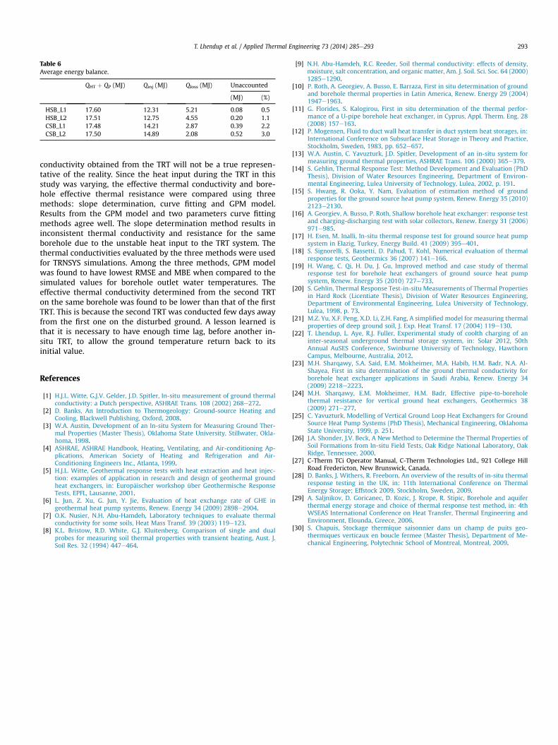
In the HSB, the average heat loss is about 30% while the averageheat injected into the ground is 70%. In the CSB, the average heatloss is 17%while the average heat injected is 81%. The summation ofheat transfer in HSB is 100% while it is about 98% in the CSB. Thedifference could be attributed to the uncertainties in the temper-ature sensors and the measuring instruments. In all the loops thereis some energy unaccounted for as shown in Table 6. The unac-counted energy is within the measurement uncertainties. There-fore, Qinj, calculated using Equation (8), is a true representative ofthe energy injected into the ground.
7. Conclusions
In-situ thermal response tests have been conducted on twoboreholes with a view to use for inter-seasonal heat and coolthstorage in Melbourne. A total of four TRT (two on each borehole)were performed on the two 40 m deep boreholes. From the fourTRT, it can be concluded that it is important to maintain constantpower input during the in-situ tests. If not the effective thermal
Fig. 21. Fraction of heat injected and lost during TRT on CSB.
T. Lhendup et al. / Applied Thermal Engineering 73 (2014) 285e293 293
conductivity obtained from the TRT will not be a true represen-tative of the reality. Since the heat input during the TRT in thisstudy was varying, the effective thermal conductivity and bore-hole effective thermal resistance were compared using threemethods: slope determination, curve fitting and GPM model.Results from the GPM model and two parameters curve fittingmethods agree well. The slope determination method results ininconsistent thermal conductivity and resistance for the sameborehole due to the unstable heat input to the TRT system. Thethermal conductivities evaluated by the three methods were usedfor TRNSYS simulations. Among the three methods, GPM modelwas found to have lowest RMSE and MBE when compared to thesimulated values for borehole outlet water temperatures. Theeffective thermal conductivity determined from the second TRTon the same borehole was found to be lower than that of the firstTRT. This is because the second TRT was conducted few days awayfrom the first one on the disturbed ground. A lesson learned isthat it is necessary to have enough time lag, before another in-situ TRT, to allow the ground temperature return back to itsinitial value.
References
[1] H.J.L. Witte, G.J.V. Gelder, J.D. Spitler, In-situ measurement of ground thermalconductivity: a Dutch perspective, ASHRAE Trans. 108 (2002) 268e272.
[2] D. Banks, An Introduction to Thermogeology: Ground-source Heating andCooling, Blackwell Publishing, Oxford, 2008.
[3] W.A. Austin, Development of an In-situ System for Measuring Ground Ther-mal Properties (Master Thesis), Oklahoma State University, Stillwater, Okla-homa, 1998.
[4] ASHRAE, ASHRAE Handbook, Heating, Ventilating, and Air-conditioning Ap-plications, American Society of Heating and Refrigeration and Air-Conditioning Engineers Inc., Atlanta, 1999.
[5] H.J.L. Witte, Geothermal response tests with heat extraction and heat injec-tion: examples of application in research and design of geothermal groundheat exchangers, in: Europ€aischer workshop über Geothermische ResponseTests, EPFL, Lausanne, 2001.
[6] L. Jun, Z. Xu, G. Jun, Y. Jie, Evaluation of heat exchange rate of GHE ingeothermal heat pump systems, Renew. Energy 34 (2009) 2898e2904.
[7] O.K. Nusier, N.H. Abu-Hamdeh, Laboratory techniques to evaluate thermalconductivity for some soils, Heat Mass Transf. 39 (2003) 119e123.
[8] K.L. Bristow, R.D. White, G.J. Kluitenberg, Comparison of single and dualprobes for measuring soil thermal properties with transient heating, Aust. J.Soil Res. 32 (1994) 447e464.
[9] N.H. Abu-Hamdeh, R.C. Reeder, Soil thermal conductivity: effects of density,moisture, salt concentration, and organic matter, Am. J. Soil. Sci. Soc. 64 (2000)1285e1290.
[10] P. Roth, A. Georgiev, A. Busso, E. Barraza, First in situ determination of groundand borehole thermal properties in Latin America, Renew. Energy 29 (2004)1947e1963.
[11] G. Florides, S. Kalogirou, First in situ determination of the thermal perfor-mance of a U-pipe borehole heat exchanger, in Cyprus, Appl. Therm. Eng. 28(2008) 157e163.
[12] P. Mogensen, Fluid to duct wall heat transfer in duct system heat storages, in:International Conference on Subsurface Heat Storage in Theory and Practice,Stockholm, Sweden, 1983, pp. 652e657.
[13] W.A. Austin, C. Yavuzturk, J.D. Spitler, Development of an in-situ system formeasuring ground thermal properties, ASHRAE Trans. 106 (2000) 365e379.
[14] S. Gehlin, Thermal Response Test: Method Development and Evaluation (PhDThesis), Division of Water Resources Engineering, Department of Environ-mental Engineering, Lulea University of Technology, Lulea, 2002, p. 191.
[15] S. Hwang, R. Ooka, Y. Nam, Evaluation of estimation method of groundproperties for the ground source heat pump system, Renew. Energy 35 (2010)2123e2130.
[16] A. Georgiev, A. Busso, P. Roth, Shallow borehole heat exchanger: response testand charging-discharging test with solar collectors, Renew. Energy 31 (2006)971e985.
[17] H. Esen, M. Inalli, In-situ thermal response test for ground source heat pumpsystem in Elazig, Turkey, Energy Build. 41 (2009) 395e401.
[18] S. Signorelli, S. Bassetti, D. Pahud, T. Kohl, Numerical evaluation of thermalresponse tests, Geothermics 36 (2007) 141e166.
[19] H. Wang, C. Qi, H. Du, J. Gu, Improved method and case study of thermalresponse test for borehole heat exchangers of ground source heat pumpsystem, Renew. Energy 35 (2010) 727e733.
[20] S. Gehlin, Thermal Response Test-in-situ Measurements of Thermal Propertiesin Hard Rock (Licentiate Thesis), Division of Water Resources Engineering,Department of Environmental Engineering, Lulea University of Technology,Lulea, 1998, p. 73.
[21] M.Z. Yu, X.F. Peng, X.D. Li, Z.H. Fang, A simplified model for measuring thermalproperties of deep ground soil, J. Exp. Heat Transf. 17 (2004) 119e130.
[22] T. Lhendup, L. Aye, R.J. Fuller, Experimental study of coolth charging of aninter-seasonal underground thermal storage system, in: Solar 2012, 50thAnnual AuSES Conference, Swinburne University of Technology, HawthornCampus, Melbourne, Australia, 2012.
[23] M.H. Sharqawy, S.A. Said, E.M. Mokheimer, M.A. Habib, H.M. Badr, N.A. Al-Shayea, First in situ determination of the ground thermal conductivity forborehole heat exchanger applications in Saudi Arabia, Renew. Energy 34(2009) 2218e2223.
[25] C. Yavuzturk, Modelling of Vertical Ground Loop Heat Exchangers for GroundSource Heat Pump Systems (PhD Thesis), Mechanical Engineering, OklahomaState University, 1999, p. 251.
[26] J.A. Shonder, J.V. Beck, A New Method to Determine the Thermal Properties ofSoil Formations from In-situ Field Tests, Oak Ridge National Laboratory, OakRidge, Tennessee, 2000.
[27] C-Therm TCi Operator Manual, C-Therm Technologies Ltd., 921 College HillRoad Fredericton, New Brunswick, Canada.
[28] D. Banks, J. Withers, R. Freeborn, An overview of the results of in-situ thermalresponse testing in the UK, in: 11th International Conference on ThermalEnergy Storage; Effstock 2009, Stockholm, Sweden, 2009.
[29] A. Saljnikov, D. Goricanec, D. Kozic, J. Krope, R. Stipic, Borehole and aquiferthermal energy storage and choice of thermal response test method, in: 4thWSEAS International Conference on Heat Transfer, Thermal Engineering andEnvironment, Elounda, Greece, 2006.
[30] S. Chapuis, Stockage thermique saisonnier dans un champ de puits geo-thermiques verticaux en boucle fermee (Master Thesis), Department of Me-chanical Engineering, Polytechnic School of Montreal, Montreal, 2009.