ORIGINAL PAPER

Increasing resolution of climate assessment and projectionof temperature and precipitation in an alpine area

Emanuele Eccel & Rodica Tomozeiu

Received: 1 October 2013 /Accepted: 20 May 2014# Springer-Verlag Wien 2014

Abstract In mountain regions, important differences inthe time trends of climate series can be detected evenwithin relatively small areas, leading to uncertaintywhen assessing climate change. The paper deals with astructured algorithm for high-resolution downscaling ofclimate characterisation in a region (precipitation andtemperature), leading to a twofold application: increas-ing spatial resolution of past climate definition for thearea and attaining high-resolution downscaling for cli-mate projections. In the first stage, multi-variate analysis(‘partial least squares’ regression) was applied to anumber of time series (10) in order to obtain climateaverages for a larger number of sites. Predictions madewith single-site values (such as seasonal means) can insome cases be improved by applying ‘random perturba-tion’ of the value and averaging single predictions inthe ensemble. This analysis laid the foundation forimplementing the same technique to the output of sta-tistical downscaling of multi-model climate projections.Climate shift in the study area (Trentino), located in thenorth-eastern Italian Alps, was simulated for two 30-year time windows: 2021–2050 and 2071–2099. Pro-gressive warming is predicted, being stronger in thesummer, along with a mixed, seasonally differentiatedtrend for precipitation.

1 Introduction

Variability in space is often overlooked in climatic changeanalyses. When several time series are analysed over the samesurvey period, important differences in time trends can bedetected even within relatively small areas (Begert et al.2005). If only a limited number of instrumental series areavailable, confidence in inferring general climate signals overthe area is reduced. This is even more true in the Alpine areas,where local climate features are determined by station altitude,slope, aspect, position with respect to dominant winds,continentality effects, type of soil cover, etc. Böhm et al.(2001) showed how different data sources may give rise todifferent climatic trends, particularly when values are griddedover complex-terrain regions (namely, the Alps). Typical stan-dard errors when estimating time trends for many decades arein the order of 10–20 % or more of the trend (Brunetti et al.2009a; Simolo et al. 2010). Fischer et al. (2012) tackled theissue of assessing the pattern of climate change over a com-plex area (Switzerland) using a Bayesian multi-model ap-proach. In the same area investigated in this study, Eccelet al. (2012) showed that the standard deviation of time trendsfor 50-year minimum temperature series was of the samemagnitude as the trend itself (much less for maximum tem-perature, thanks only to higher rates of time trends) after serieshomogenisation, The authors argued that such values, al-though lower as compared to raw series, are still able to causeuncertainty in the assessment of climatic change occurringover the area. In particular, when the average trend is weak,signs of single-series trends may be different from the prevail-ing trend in the area, albeit not generally in a significantmanner.

The aforementioned arguments explain why a dense refer-ence station network is desirable when high-resolution analy-sis has to be carried out in a region, for instance, when spatialinterpolation of values is to be carried out (Ciccarelli et al.

E. Eccel (*)Sustainable Agro-ecosystems and Bioresources Department,IASMA Research and Innovation Centre, Fondazione EdmundMach, Via E. Mach 1, 38010 San Michele all’Adige, Italye-mail: emanuele.eccel@fmach.it

R. TomozeiuServ. IdroMeteoClima, ARPA Emilia-Romagna, V.le Silvani, 6,40122 Bologna, Italy

Theor Appl ClimatolDOI 10.1007/s00704-014-1181-4

2008; Haylock et al. 2008). This is particularly importantwhen geo-topographic features are taken into account asdrivers for spatial interpolation (Brugnara et al. 2011; DiPiazza et al 2011). However, this need is often in contrast withthe availability of a satisfactory number of series, both for pastclimatology and in the case of climate projections. In theformer case, the desirable WMO standard is a 30-year longtime series, and the reference period is still in many cases1961–1990, although 10- and 20-year-shifted periods (1971–2000 and 1981–2010) are now more frequently used than inthe past. Weather network coverage has increased widelyalmost everywhere in the last 50 years, perhaps with theexception of rain-gauge networks, which were establishedearlier, so the consistency of meteorological networks suitablefor assessing climate features in the period 1961–1990 waspoorer than for the more recent 1981–2010 30-year period.Hence, if a very short measurement gap can be accepted forclimate analysis of series, the number of series available forclimatology is lower, as they are further away in time. As asolution to this problem, estimation of climate features in areaspoorly covered by climate series in the time domain has beenproposed, for example, by Sansom and Tait (2004), whosuggested an interpolating approach; Mitchell and Jones(2005) made use of reference series constructed withneighbouring ones; New et al. (2000) applied the ‘anomaly’approach (New et al. 1999) to best exploit the availability ofdata in space and time as compared to a standard referenceperiod. For the Italian network, the problem was tackled fortemperature by Brunetti et al. (2009b) to estimate a seculartemperature anomaly record and for precipitation by Brunettiet al. (2009c).

On the other hand, in order to increase the resolution and toobtain detailed climate scenarios, optimal coverage by climat-ic series is also important in projections of future scenarios, inwhich time-consuming statistical downscaling (SD) can beapplied to a limited number of instrumental sites in order toconstruct seasonal projections. Downscaling tools depend onlarge-scale circulation variables as simulated by global climatemodels (GCMs), so their importance in increasing the spatialresolution of climate change projections also depends on thequality of the GCM simulations (Maraun et al. 2010). Statis-tical methods are based on empirical relations between ob-served large-scale variables (predictors) and local variables(predictands). In general, atmospheric fields are betterreproduced by GCMs at upper levels than at the surface;therefore, the former are preferred as predictors in downscal-ing processes.

The aim of this paper is to illustrate a technique to increaseas much as possible the number of sites where the climate ofan area can be assessed, starting from a lower number ofknown values. The method is proposed for application toeither instrumental (‘reference’) or simulated (projection) se-ries from GCMs. The method involves inferring climatic

features at sites where no measured values can be averaged,either because the instrumental series is incomplete or evenmissing for the desired period (as in the case of past climatol-ogy)—or because dense, site-specific statistical downscalingis not fully available (in the case of future projections). Themethod applies partial least square regression technique—amulti-variate approach based on principal component analysisalgorithms—in which the predictors are the available values atsome sites and the predictands are the values at the other sites,in the same period. The method requires the partial overlap-ping of time series in both predictands and predictors. Theresults of past climate reconstruction and of downscaling offuture projections are discussed in the light of this enhancedavailability of climate information in the region and comparedto the results obtained in previous works.

2 Methods

2.1 Geographical area, meteorological series and processing

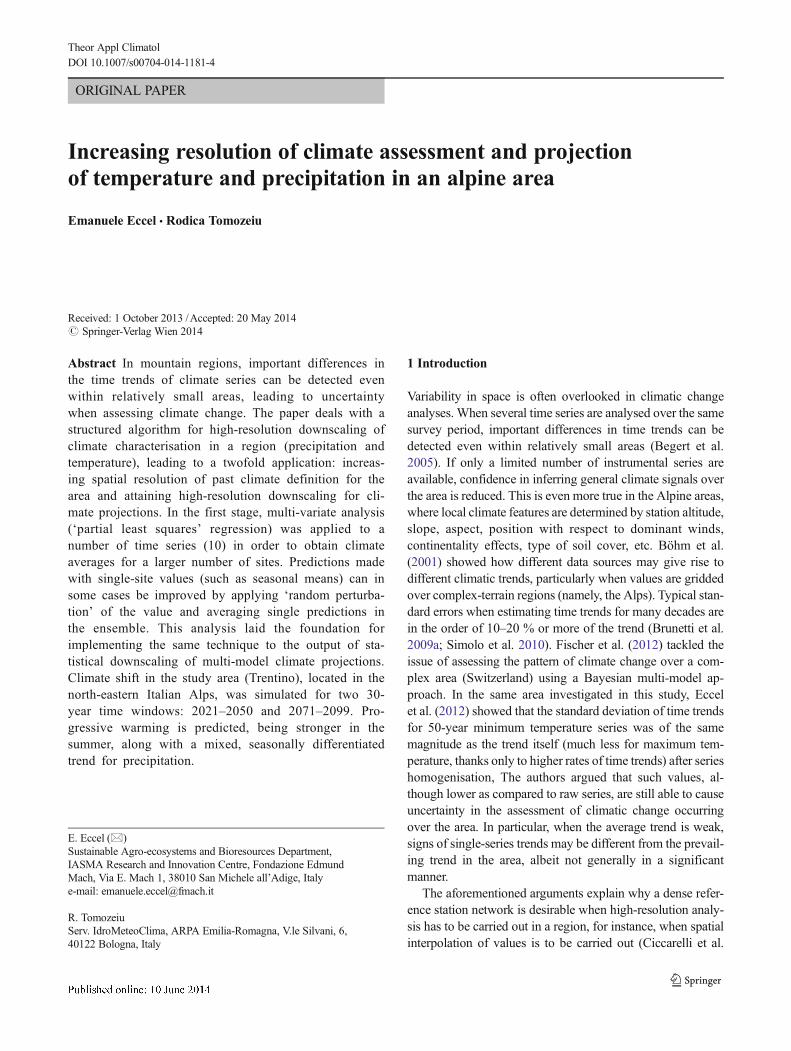
Climatic downscaling was carried out for a mountain region inthe Italian Alps (Trentino) and the neighbouring area (Fig. 1).The morphology of the area is characterised by a valleysystem, with altitudes between 70 m a.s.l. (Lake Garda) and3,769 m (the summit of the Cevedale). The area covered bythe weather station network can be ascribed mostly to the‘Cfb’Köppen class (‘temperate, middle latitudes climate, withno dry season’). In more elevated, mountain areas, the classshifts to ‘Dfc’ (‘microthermal climate, humid all year round’).Precipitation is more abundant in two peak periods, in autumn(main) and in spring (secondary). In general, the relativesummer minimum is little accentuated, so that in some moun-tain areas, rainfall usually peaks in summer (Eccel andSaibanti 2007).

The SD of climatic records, as well as sub-downscalingprocessing, was carried out with seasonal aggregation of data(where winter is DJF and so on). The series underwent pre-liminary gap filling, homogenisation and correction for sys-tematic snowfall underestimation, as described in Eccel et al.2012. Only series with a minimum of 25 annual values foreach season (83 % of series length) were taken into account tocalculate climatic normals for the reference period 1961–1990; otherwise, the corresponding value was set to missingand the site was considered as a predictand for the sub-downscaling algorithm.

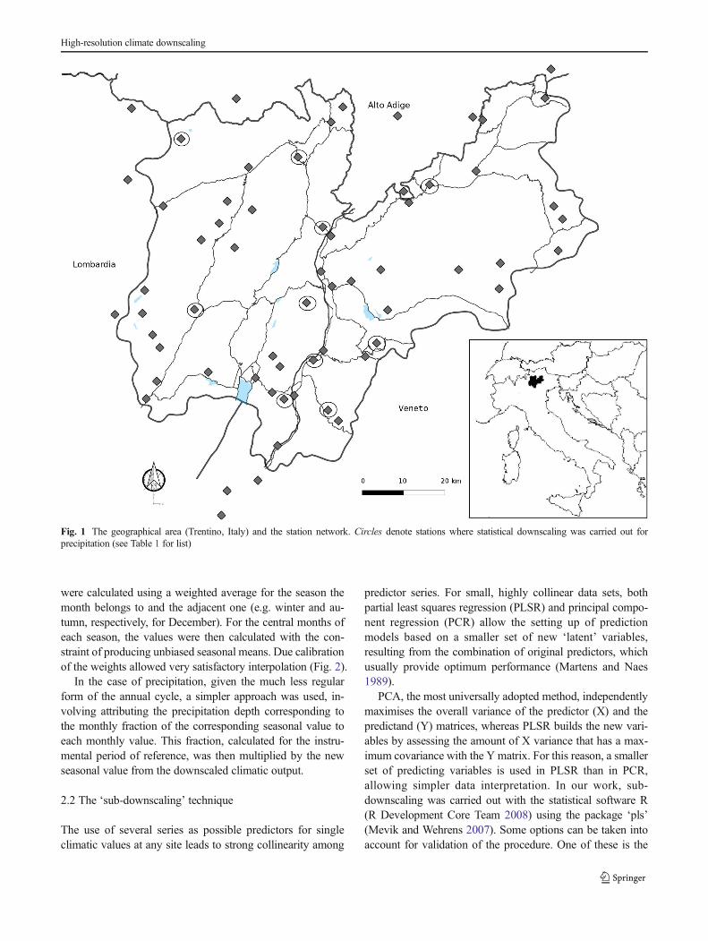
Finally, seasonal values were interpolated to monthlyvalues by using different algorithms for temperature and pre-cipitation. In the former case, spline interpolation was carriedout. In order to avoid non-realistic steps between one seasonand another, an adjustment was made to the ‘outer’months ofeach season (e.g. December and February for winter, Marchand May for spring and so on): the values for these months

E. Eccel, R. Tomozeiu

were calculated using a weighted average for the season themonth belongs to and the adjacent one (e.g. winter and au-tumn, respectively, for December). For the central months ofeach season, the values were then calculated with the con-straint of producing unbiased seasonal means. Due calibrationof the weights allowed very satisfactory interpolation (Fig. 2).

In the case of precipitation, given the much less regularform of the annual cycle, a simpler approach was used, in-volving attributing the precipitation depth corresponding tothe monthly fraction of the corresponding seasonal value toeach monthly value. This fraction, calculated for the instru-mental period of reference, was then multiplied by the newseasonal value from the downscaled climatic output.

2.2 The ‘sub-downscaling’ technique

The use of several series as possible predictors for singleclimatic values at any site leads to strong collinearity among

predictor series. For small, highly collinear data sets, bothpartial least squares regression (PLSR) and principal compo-nent regression (PCR) allow the setting up of predictionmodels based on a smaller set of new ‘latent’ variables,resulting from the combination of original predictors, whichusually provide optimum performance (Martens and Naes1989).

PCA, the most universally adopted method, independentlymaximises the overall variance of the predictor (X) and thepredictand (Y) matrices, whereas PLSR builds the new vari-ables by assessing the amount of X variance that has a max-imum covariance with the Y matrix. For this reason, a smallerset of predicting variables is used in PLSR than in PCR,allowing simpler data interpretation. In our work, sub-downscaling was carried out with the statistical software R(R Development Core Team 2008) using the package ‘pls’(Mevik and Wehrens 2007). Some options can be taken intoaccount for validation of the procedure. One of these is the

Fig. 1 The geographical area (Trentino, Italy) and the station network. Circles denote stations where statistical downscaling was carried out forprecipitation (see Table 1 for list)

High-resolution climate downscaling

leave-one-out method, which involves using all the recordsbut one, in turn, to calibrate the model, and subsequentlyperforming the prediction for the excluded record. This algo-rithm is particularly suitable when the sample is not too large,as in this study. The procedure is repeated, leaving out eachelement one by one. The performance of the model is assessedusing the root-mean-square error, according to which theoptimum number of components is chosen. In order to repro-duce identical processing conditions for climatic reconstruc-tion of missing series in the past, the same 10 series used forfuture projections (in the latter case as the output of statisticaldownscaling) were chosen as predictors, excluding other in-strumental series that would have been available in this case.A simple diagram representing the processing flow of the‘sub-downscaling’ algorithm is given in Fig. 3. The generalequation for this process is as follows:

Y!¼ pls X

!� �ð1Þ

where Y!

is the predictand vector (e.g. the seasonal values forminimum temperature), whose length is the number ofpredictand series (45 or 33 for precipitation and temperature,respectively) minus the number of predictor series (10), pls isthe partial least squares algorithm (R library ‘pls’) and X

!� �

is the predictor matrix (i.e. either a 10×1 vector of seasonal

precipitation values or a 10×2 matrix of seasonal minimumand maximum temperature values, one column each).

When used to predict climate for a number of sites, predic-tors are single, average climate values for each climate period,such as mean seasonal temperature or mean seasonal precip-itation depth; in this case study, there were 10 predictors (SDoutput over the selected sites—see Section 2.3), which weredoubled in the case of temperature, with both minimum andmaximum values being taken into account as predictors. Thepredictands (one predictand per site) were 45 and 33 forprecipitation and temperature, respectively. So, there wereone (for precipitation) or two (for temperature) numbers foreach of the 10 predictors, expressing the projected values asresulting from statistical downscaling. The use of additionalexogenous predictors (precipitation for estimating tempera-ture and vice-versa) was attempted, but was discarded owingto the absence of improvement in the results, as expected.

The multi-variate sub-downscaling technique should pro-duce a prediction expressing the mean over each 30-yearperiod, on the basis of one value only (or a pair of min–maxvalues for temperature) for each predictor. The robustness ofsuch a prediction can be considered questionable. To avoidthis shortcoming, a stochastic series of predictor values wasgenerated, and the final prediction obtained by averaging theset of realisations. This approach was described as ‘ensemblerandom perturbation’ (ERP). In our implementation of ERP,

Fig. 2 Example of monthlyinterpolation of seasonalminimum temperature values(station T0001)

E. Eccel, R. Tomozeiu

the original predictor vector (either 10 single values, or10min–max temperature pairs) gave rise to 200 predictor sets.Each set of 10 predictors (10×2 for temperature) was calcu-lated according to one random number ~N(0,1). This samerandom number was used to generate one set of predictorvalues, by applying each site-specific mean and standarddeviation to the normalised value, so that each value in oneprediction set had the same position in its own probabilityfunction, i.e. one of the 200 predictor sets could express, forexample, seasonal precipitation depth corresponding to a ran-dom probability, ‘p’, of occurrence for each site. In this way,the ERP prediction was the result of the average for 200realisations, whose predictors had the same mean as the orig-inal values, perturbation being a ‘white noise’.

In this case, Eq. 1 becomes the following:

Y!¼

Xi¼1

200pls X

!þ Ni 0; σ!X

� �� �ð1aÞ

where Ni is the ‘random perturbation’ vector function, whoseresult is a random vector of values generated from normaldistribution with a null mean and whose σX’s are the standarddeviations of the 10 predictors.

2.3 The future climate baseline scenario: statisticaldownscaling from GCMs

In the case of future projections, the method requires knowl-edge of downscaled climate scenarios at a limited number ofsites. The statistical downscaling scheme applied in this workwas set up in the framework of the ENSEMBLES project(Tomozeiu et al 2013a) and focused on northern Italy. TheA1B scenario of IPCC’s Special Report on Emission Scenar-ios (SRES) was used, and the projections were constructed

over the periods 2021–2050 and 2071–2099, as compared to1961–1990. The statistical technique follows the perfect-progapproach, in which the links between large-scale (predictors)and local scale (predictands) are detected from observed datathrough canonical correlation analyses (CCA). The local datasets used in the algorithm calibration include station data fromTrentino, some of which were already included in the workdeveloped in northern Italy. In this work, the missing temper-ature stations were included in the observed data set and newcalibration was carried out. Furthermore, a new setup for thescheme was carried out for precipitation depth and number ofdays with precipitation. Then, the most effective SD schemesfor both temperature and precipitation were fed with predic-tors simulated using GCMs-ENSEMBLES (http://ensembles.wdc-climate.de)-STREAM1, in order to estimate thecorresponding climate signal at station level. Fowler et al.(2007) and van der Linden and Mitchell (2009) suggest amulti-model approach to increase the robustness of climatechange assessment. Thus, in order to construct a multi-modelapproach for Trentino, in this study, runs were used from thefollowing modelling groups: INGV, NERSC, FUB, IPSL,METOHC (2 runs) and MPIMET + DMI. Details concerningGCM large-scale field simulations were presented by Van derLinden and Mitchell (2009) in the Research Theme RT2A ofthe ENSEMBLES project (http://ensembles-eu.metoffice.com/results.html).

The predictors tested in the setup of the SD model arelarge-scale atmospheric quantities: mean sea level pressure(MSLP), 500 hPa geopotential height (Z500) and temperatureat 850 hPa (T850). The links between these fields and localclimate variability have already been investigated byTomozeiu et al. (2013a), in northern Italy and in small singleareas in the Italian peninsula (Tomozeiu et al. 2013b), in orderto construct seasonal scenarios for temperature and

Fig. 3 Workflow process for the‘sub-downscaling’ algorithm

High-resolution climate downscaling

precipitation. As regards the predictands, these were the sea-sonal averages of air temperature: minimum (Tn) and maxi-mum (Tx), precipitation depth (Prec) and number of precipi-tation days (ddP—days with precipitation ≥1mm), recorded at10 selected stations in Trentino (Fig. 1 and Table 1). In orderto reduce the noise of predictands and predictors involved inthe setup of the SD scheme, principal component analysis—PCA (Wilks 2006)—was carried out on the de-trended dataand only principal components that explained most of the totalobserved variance were retained in the CCA analysis (VonStorch 1995). The CCA method simultaneously identifiesmodes of both predictor and predictand pairs that maximisetheir temporal correlation. A subset of these pairs is then usedin the multi-variate linear model in order to estimatepredictand anomalies from the predictor anomaly field. Thenumber of PCs used in canonical correlation analysis and thenumber of canonical correlation patterns used in the regres-sion model influence the performance of the CCARegscheme.

Evaluation of SD skill was carried out using cross-validation. The whole interval for the data observed, namely,1958–2002, was divided into two homogeneous periods: the1958–1978+1996–2002 periods were used to construct themodel; the 1979–1995 period was used in the validationphase. The correlation coefficients calculated between ob-served and downscaled time series and the bias were the mainstatistics used to evaluate the performance of the SD scheme.

3 Results and discussion

3.1 Climatic reconstruction for sites with incomplete series

For the standard 1961–1990 climatic period, 22 out of a totalof 51 available stations in the network met the requirement on

the minimum length of the series (25 years). These seriesformed the instrumental climatic core, on which the sub-downscaling algorithm was calibrated. The other 29 serieswere the predictands, to which the ‘predict’ function of R-package pls was actually applied. The skill of the predictionmodel was calculated on the 22 ‘complete’ series. For each ofthese, the prediction biases (simulated minus measured singleseasonal values) were calculated for three reference periods:the standard 1961–1990, the alternative 1971–2000 and thelatest available 30 years in the instrumental series, 1978–2007.

An acceptance criterion was applied to sub-downscaling,based on the correlation and error statistics calculated for theobserved-simulated series. For each prediction session, thecoefficient of determination is calculated by the pls package as

R2m ¼ 1−

SSE

SSTð2Þ

where SSE is the sum of squared errors for the cross-validatedprediction and SST is the sum of the squared deviations of theobservations from their mean (note that Rm

2 is not the square ofPearson’s correlation coefficient and that it has a negativevalue if the sum of squares of model residuals is higher thanthe sum of the squared deviations). Predictions were acceptedwith a Rm

2 threshold of 0.45.In Fig. 4, examples of predictions from two pairs of series

are reported, with the relevant Rm2 values. In the example,

predictions for series T0204, autumn (temperature) and seriesT0103, summer (precipitation) were rejected, due to the poorresults. On the contrary, excellent performance was obtainedfor temperature with the series B7810, summer, and for pre-cipitation with the series T0110, spring. As can be seen,different performances can be obtained for different seasonsfor the same series.

Table 1 List of stations used instatistical downscaling (for tem-perature, precipitation or both)

Station Name Elevation (m a.s.l.) Temperature/precipitation

T0001 Pergine Valsugana 457 T

T0018 Pieve Tesino 775 T P

T0064 Peio 1,565 T P

T0083 Cles 665 T P

T0090 Mezzolombardo 225 T P

T0092 Pian Fedaia 2,040 T

T0129 Trento Laste 312 T

T0210 Folgaria 1,140 T P

T0327 Monte Bondone 1,552 T P

T0367 Cavalese 958 T P

T0152 Brentonico 693 P

T0154 Ala 165 P

T0179 Tione 539 P

E. Eccel, R. Tomozeiu

A further check was done on relative error for precipitationalone, calculated as the usual root-mean-square error of pre-diction (RMSEP) divided by the average value of seasonalprecipitation for each series (‘relative RMSEP’). Predictionswere accepted with a relative RMSEP threshold of 0.25.

Assessment of the prediction skill of sub-downscalingcan be given by the correlation (coefficient of determina-tion Rm

2—eq. 2) between annual series of seasonal

observations and predictions for a hindcast period, calcu-lated using the pls library with the Leave-One-Out (LOO)approach. In Tables 2 and 3, the quantiles of Rm

2 andrelative RMSEP (precipitation only) are shown for the 30-year period 1978–2007—within the data set, the one withthe highest level of completeness in the series. The distri-bution refers to the sample of all predictand series andshows satisfactory skill in the vast majority of cases.

Fig. 4 Examples of predicted vs. measured values for past climate at two pairs of stations with partial least square regression (pls). a temperature (Tnminimum, Tx maximum). b precipitation

High-resolution climate downscaling

Instead of generating predictions from single average cli-matic values (in this case with the ‘ensemble random pertur-bation’ option), means can be calculated by averaging thesingle annual predictions for each season over the period. InTable 4, a summary of results is given for the period 1978–2007. The sample is made up of the values for all thepredictand series. It can be seen that the acceptance standardis generally met in at least 90 % of stations and that in general,this approach functions even better than prediction from singleclimatic values for each station. Of course, this approachcannot be used for projections if only the period average isgiven as an input.

The two rejection thresholds allow a number of predictionrejections from 0 to 20 %, according to the season and vari-able, as can be seen in Table 5. For precipitation, the numberof rejections shows only a slight increase when the additional

check on the relative RMSEP is added to the condition on Rm2 .

The adoption of the ERP technique in temperature sub-downscaling did not significantly improve the results andwas not applied; on the contrary, for precipitation, the percent-age of projections where this method had the chance to im-prove prediction ranged from 16 to 38 %.

The goodness of climatic reconstruction was calculated bycomparing the true climatic values, when available, with theestimated values. For temperature, biases of sub-downscalingwere always within the [−0.10 K÷+0.20 K] range for all pastclimatic periods, with medians always equal to 0.0 K. Forprecipitation, the medians were always within a ±1 % range,

Table 2 Sub-downscaling model skills (Leave-One-Out) for precipita-tion, period 1978–2007

DJF MAM JJA SON

Rm2 (Eq. 2)

Min 0.42 −0.11 −0.08 0.52

25 % 0.72 0.63 0.49 0.82

50 % 0.82 0.80 0.55 0.88

75 % 0.89 0.86 0.66 0.91

Max 0.95 0.97 0.79 0.96

Relative RMSEP (RMSEP/mean seasonal value)

Min 0.05 0.04 0.10 0.11

25 % 0.09 0.11 0.14 0.14

50 % 0.11 0.13 0.16 0.17

75 % 0.14 0.18 0.18 0.20

Max 0.23 0.69 0.43 0.37

Table 3 Sub-downscaling model skills (Leave-One-Out) for tempera-ture, period 1978–2007: Rm

2 (Eq. 2)

DJF MAM JJA SON

Minimum temperature

Min 0.47 0.11 0.03 0.38

25 % 0.67 0.60 0.51 0.63

50 % 0.77 0.74 0.64 0.72

75 % 0.85 0.80 0.76 0.82

Max 0.96 0.93 0.99 0.95

Maximum temperature

Min 0.41 0.35 0.61 0.27

25 % 0.74 0.74 0.71 0.56

50 % 0.83 0.80 0.84 0.68

75 % 0.88 0.87 0.90 0.79

Max 0.92 0.94 0.97 0.97

Table 4 Sub-downscaling model skills (Rm2—Eq. 2). Statistics for full

period means

DJF MAM JJA SON

Precipitation

Min 0.61 0.43 0.17 0.34

10 % 0.73 0.60 0.48 0.80

25 % 0.83 0.81 0.60 0.89

50 % 0.91 0.87 0.70 0.93

75 % 0.94 0.91 0.77 0.95

Minimum temperature

Min 0.58 0.24 0.12 0.02

10 % 0.75 0.63 0.57 0.62

25 % 0.84 0.81 0.68 0.79

50 % 0.90 0.88 0.77 0.88

75 % 0.94 0.91 0.91 0.92

Maximum temperature

Min 0.24 0.64 0.68 0.04

10 % 0.81 0.81 0.74 0.68

25 % 0.88 0.86 0.84 0.81

50 % 0.92 0.92 0.92 0.89

75 % 0.95 0.96 0.97 0.93

Table 5 Rows 1–4: fraction of the number of seasonal predictionsrejected due to poor performance in the coefficient of determination(Rm

2) and in the relative root-mean-square error of prediction(RMSErel—‘P’ only). Row 5: fraction of the number of predictions wherethe ‘ensemble random perturbation’ algorithm (ERP) is preferable to thesimple prediction

Row—var.

Number of sites Condition DJF MAM JJA SON

1. Tn 33 Rm2 0.00 0.06 0.18 0.03

2. Tx 33 Rm2 0.03 0.03 0.00 0.15

3. P 45 Rm2 0.04 0.13 0.20 0.00

4. P 45 Rm2+RMSErel 0.04 0.16 0.20 0.04

5. P 45 ERP 0.16 0.16 0.24 0.38

E. Eccel, R. Tomozeiu

with inter-quartile ranges (IQRs) mostly within the ±2÷3 %and close to 4 % in one case only (winter, 1978–2007),probably driven by some outlier. It was ascertained that theoutliers could be generally ascribed to stations at the border ofthe domain. Hence, the inclusion of stations outside the area ofinterest is likely to avoid, at least partially, the bias of estimat-ed values inside the area. In general, errors for the estimationof means at incomplete sites could be even lower, if a highernumber of stations could be used as predictors. However, forthe sake of homogeneity, this approach was not used becauseit would have been inapplicable in the case of predictions.

3.2 Application to high-resolution climate projections in asmall mountain region

3.2.1 Setup of SD schemes at seasonal level

SD setup was done by comparing various combinations ofpredictors in order to select models that minimise bias andmaximise the explained variance between downscaled andobserved data for each variable and for each season. Resultson the selection of predictors confirm the findings obtained forprojections in different Italian areas (Tomozeiu et al. 2013a,b). For temperature, the best model skill was obtained withtemperature at 850 hPa (T850), while for both P and ddP,mean sea level pressure was in general the best predictor.Cacciamani et al. (1994) and Toreti et al. (2010) highlightthe robustness of patterns linking large-scale atmosphericvariability with local climate variability over the Italian pen-insula, affecting the performance of SD implementation.

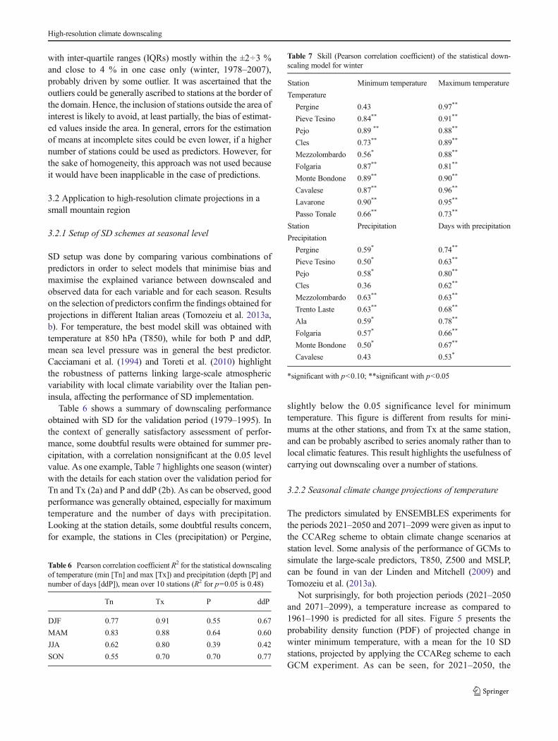
Table 6 shows a summary of downscaling performanceobtained with SD for the validation period (1979–1995). Inthe context of generally satisfactory assessment of perfor-mance, some doubtful results were obtained for summer pre-cipitation, with a correlation nonsignificant at the 0.05 levelvalue. As one example, Table 7 highlights one season (winter)with the details for each station over the validation period forTn and Tx (2a) and P and ddP (2b). As can be observed, goodperformance was generally obtained, especially for maximumtemperature and the number of days with precipitation.Looking at the station details, some doubtful results concern,for example, the stations in Cles (precipitation) or Pergine,

slightly below the 0.05 significance level for minimumtemperature. This figure is different from results for mini-mums at the other stations, and from Tx at the same station,and can be probably ascribed to series anomaly rather than tolocal climatic features. This result highlights the usefulness ofcarrying out downscaling over a number of stations.

3.2.2 Seasonal climate change projections of temperature

The predictors simulated by ENSEMBLES experiments forthe periods 2021–2050 and 2071–2099 were given as input tothe CCAReg scheme to obtain climate change scenarios atstation level. Some analysis of the performance of GCMs tosimulate the large-scale predictors, T850, Z500 and MSLP,can be found in van der Linden and Mitchell (2009) andTomozeiu et al. (2013a).

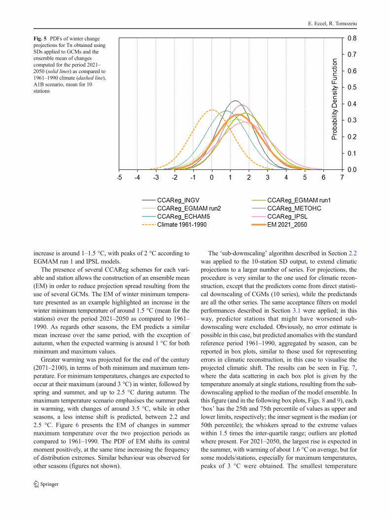
Not surprisingly, for both projection periods (2021–2050and 2071–2099), a temperature increase as compared to1961–1990 is predicted for all sites. Figure 5 presents theprobability density function (PDF) of projected change inwinter minimum temperature, with a mean for the 10 SDstations, projected by applying the CCAReg scheme to eachGCM experiment. As can be seen, for 2021–2050, the

Table 6 Pearson correlation coefficient R2 for the statistical downscalingof temperature (min [Tn] and max [Tx]) and precipitation (depth [P] andnumber of days [ddP]), mean over 10 stations (R2 for p=0.05 is 0.48)

Tn Tx P ddP

DJF 0.77 0.91 0.55 0.67

MAM 0.83 0.88 0.64 0.60

JJA 0.62 0.80 0.39 0.42

SON 0.55 0.70 0.70 0.77

Table 7 Skill (Pearson correlation coefficient) of the statistical down-scaling model for winter

Station Minimum temperature Maximum temperature

Temperature

Pergine 0.43 0.97**

Pieve Tesino 0.84** 0.91**

Pejo 0.89 ** 0.88**

Cles 0.73** 0.89**

Mezzolombardo 0.56* 0.88**

Folgaria 0.87** 0.81**

Monte Bondone 0.89** 0.90**

Cavalese 0.87** 0.96**

Lavarone 0.90** 0.95**

Passo Tonale 0.66** 0.73**

Station Precipitation Days with precipitation

Precipitation

Pergine 0.59* 0.74**

Pieve Tesino 0.50* 0.63**

Pejo 0.58* 0.80**

Cles 0.36 0.62**

Mezzolombardo 0.63** 0.63**

Trento Laste 0.63** 0.68**

Ala 0.59* 0.78**

Folgaria 0.57* 0.66**

Monte Bondone 0.50* 0.67**

Cavalese 0.43 0.53*

*significant with p<0.10; **significant with p<0.05

High-resolution climate downscaling

increase is around 1–1.5 °C, with peaks of 2 °C according toEGMAM run 1 and IPSL models.

The presence of several CCAReg schemes for each vari-able and station allows the construction of an ensemble mean(EM) in order to reduce projection spread resulting from theuse of several GCMs. The EM of winter minimum tempera-ture presented as an example highlighted an increase in thewinter minimum temperature of around 1.5 °C (mean for thestations) over the period 2021–2050 as compared to 1961–1990. As regards other seasons, the EM predicts a similarmean increase over the same period, with the exception ofautumn, when the expected warming is around 1 °C for bothminimum and maximum values.

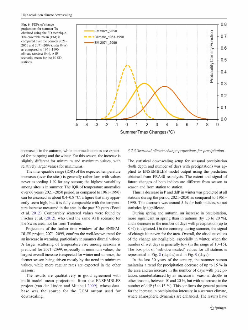
Greater warming was projected for the end of the century(2071–2100), in terms of both minimum and maximum tem-perature. For minimum temperatures, changes are expected tooccur at their maximum (around 3 °C) in winter, followed byspring and summer, and up to 2.5 °C during autumn. Themaximum temperature scenario emphasises the summer peakin warming, with changes of around 3.5 °C, while in otherseasons, a less intense shift is predicted, between 2.2 and2.5 °C. Figure 6 presents the EM of changes in summermaximum temperature over the two projection periods ascompared to 1961–1990. The PDF of EM shifts its centralmoment positively, at the same time increasing the frequencyof distribution extremes. Similar behaviour was observed forother seasons (figures not shown).

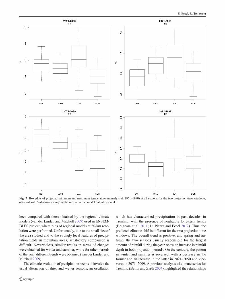
The ‘sub-downscaling’ algorithm described in Section 2.2was applied to the 10-station SD output, to extend climaticprojections to a larger number of series. For projections, theprocedure is very similar to the one used for climatic recon-struction, except that the predictors come from direct statisti-cal downscaling of CGMs (10 series), while the predictandsare all the other series. The same acceptance filters on modelperformances described in Section 3.1 were applied; in thisway, predictor stations that might have worsened sub-downscaling were excluded. Obviously, no error estimate ispossible in this case, but predicted anomalies with the standardreference period 1961–1990, aggregated by season, can bereported in box plots, similar to those used for representingerrors in climatic reconstruction, in this case to visualise theprojected climatic shift. The results can be seen in Fig. 7,where the data scattering in each box plot is given by thetemperature anomaly at single stations, resulting from the sub-downscaling applied to the median of the model ensemble. Inthis figure (and in the following box plots, Figs. 8 and 9), each‘box’ has the 25th and 75th percentile of values as upper andlower limits, respectively; the inner segment is the median (or50th percentile); the whiskers spread to the extreme valueswithin 1.5 times the inter-quartile range; outliers are plottedwhere present. For 2021–2050, the largest rise is expected inthe summer, with warming of about 1.6 °C on average, but forsome models/stations, especially for maximum temperatures,peaks of 3 °C were obtained. The smallest temperature

Fig. 5 PDFs of winter changeprojections for Tn obtained usingSDs applied to GCMs and theensemble mean of changescomputed for the period 2021–2050 (solid lines) as compared to1961–1990 climate (dashed line),A1B scenario, mean for 10stations

E. Eccel, R. Tomozeiu

increase is in the autumn, while intermediate rates are expect-ed for the spring and the winter. For this season, the increase isslightly different for minimum and maximum values, withrelatively larger values for minimums.

The inter-quartile range (IQR) of the expected temperatureincreases (over the sites) is generally rather low, with valuesnever exceeding 1 K for any season; the highest variabilityamong sites is in summer. The IQR of temperature anomaliesover 60 years (2021–2050 period, as compared to 1961–1990)can be assessed as about 0.4–0.8 °C, a figure that may appar-ently seem high, but it is fully comparable with the tempera-ture increase measured in the area in the past 50 years (Eccelet al. 2012). Comparably scattered values were found byFischer et al. (2012), who used the same A1B scenario forthe Swiss area, not far from Trentino.

Projections of the further time window of the ENSEM-BLES project, 2071–2099, confirm the well-known trend foran increase in warming, particularly in summer diurnal values.A larger scattering of temperature rise among seasons ispredicted for 2071–2099, especially in minimum values; thelargest overall increase is expected for winter and summer, theformer season being driven mostly by the trend in minimumvalues, while more regular rates are expected in the otherseasons.

The results are qualitatively in good agreement withmulti-model mean projections from the ENSEMBLESproject (van der Linden and Mitchell 2009), whose data-base was the source for the GCM output used fordownscaling.

3.2.3 Seasonal climate change projections for precipitation

The statistical downscaling setup for seasonal precipitation(both depth and number of days with precipitation) was ap-plied to ENSEMBLES model output using the predictorsobtained from ERA40 reanalysis. The extent and signal offuture changes of both indices are different from season toseason and from station to station.

Thus, a decrease in P and ddP in winter was predicted at allstations during the period 2021–2050 as compared to 1961–1990. This decrease was around 5 % for both indices, so notstatistically significant.

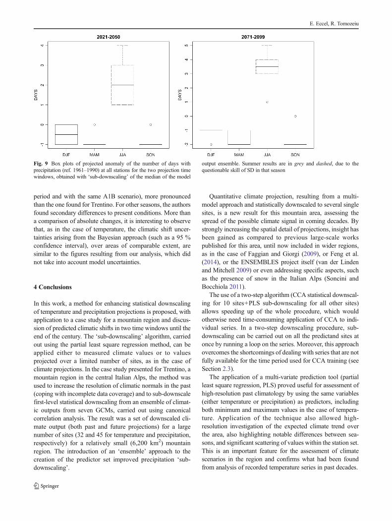
During spring and autumn, an increase in precipitation,more significant in spring than in autumn (by up to 20 %),and a decrease in the number of days with precipitation (up to8 %) is expected. On the contrary, during summer, the signalof change is uneven for the area. Overall, the absolute valuesof the change are negligible, especially in winter, when thenumber of wet days is generally low (in the range of 10–15).The box plot of ‘sub-downscaled’ values for all stations isrepresented in Fig. 8 (depths) and in Fig. 9 (days).

In the last 30 years of the century, the summer seasonmaintains a trend for precipitation decrease of up to 15 % inthe area and an increase in the number of days with precipi-tation, counterbalanced by an increase in seasonal depths inother seasons, between 10 and 20%, but with a decrease in thenumber of ddP (5 to 15 %). This confirms the general patternfor the increase in precipitation intensity in a warmer climate,where atmospheric dynamics are enhanced. The results have

Fig. 6 PDFs of changeprojections for summer Txobtained using the SD technique.The ensemble mean (EM) iscomputed over the periods 2021–2050 and 2071–2099 (solid lines)as compared to 1961–1990climate (dashed line), A1Bscenario, mean for the 10 SDstations

High-resolution climate downscaling

been compared with those obtained by the regional climatemodels (van der Linden and Mitchell 2009) used in ENSEM-BLES project, where runs of regional models at 50-km reso-lution were performed. Unfortunately, due to the small size ofthe area studied and to the strongly local features of precipi-tation fields in mountain areas, satisfactory comparison isdifficult. Nevertheless, similar results in terms of changeswere obtained for winter and summer, while for other periodsof the year, different trends were obtained (van der Linden andMitchell 2009).

The climatic evolution of precipitation seems to involve theusual alternation of drier and wetter seasons, an oscillation

which has characterised precipitation in past decades inTrentino, with the presence of negligible long-term trends(Brugnara et al. 2011; Di Piazza and Eccel 2012). Thus, thepredicted climatic shift is different for the two projection timewindows. The overall trend is positive, and spring and au-tumn, the two seasons usually responsible for the largestamount of rainfall during the year, show an increase in rainfalldepth in both projection periods. On the contrary, the patternin winter and summer is reversed, with a decrease in theformer and an increase in the latter in 2021–2050 and vice-versa in 2071–2099. A previous analysis of climate series forTrentino (Bellin and Zardi 2004) highlighted the relationships

Fig. 7 Box plots of projected minimum and maximum temperature anomaly (ref. 1961–1990) at all stations for the two projection time windows,obtained with ‘sub-downscaling’ of the median of the model output ensemble

E. Eccel, R. Tomozeiu

between large-scale, oscillatory circulation patterns and sea-sonal precipitation variability. The complexity of the rela-tionships provides a reason for the absence of continuityin the climatic signal of precipitation for the future,confirmed by the analysis of past series in the same area(Di Piazza and Eccel 2012).

An inverse correlation can be suggested between tempera-ture and precipitation in summer. At first glance, this could beconsidered odd, since higher maximum temperatures, partic-ularly in summer, could be linked to lower than average skycover at day time, leading to lower than average rainfall.However, it must be stressed that in mountain areas, a

significant amount of rainfall is enhanced by orographic airrising, and in turn by strong soil heating, leading to convectivecloud cover and rainstorms during the second part of the day.This could also explain the partial match with large-scale,multi-model mean predictions from the ENSEMBLES project(van der Linden and Mitchell 2009). For some regions ofAustria, the same inverse relationship was found betweenrainfall and temperature in recent decades, even if the patternof correlation between the two variables is much more com-plex (Auer et al. 2001). The work by Fischer et al. (2012)highlighted a clear trend for lower precipitation in summer forthe last 30 years of the century for Switzerland (for the same

Fig. 8 Box plots of projected precipitation anomaly (ref. 1961–1990) at all stations for the two projection time windows, obtained with ‘sub-downscaling’ of the median of the model output ensemble. Summer results are in grey and dashed, due to the questionable skill of SD in that season

High-resolution climate downscaling

period and with the same A1B scenario), more pronouncedthan the one found for Trentino. For other seasons, the authorsfound secondary differences to present conditions. More thana comparison of absolute changes, it is interesting to observethat, as in the case of temperature, the climatic shift uncer-tainties arising from the Bayesian approach (such as a 95 %confidence interval), over areas of comparable extent, aresimilar to the figures resulting from our analysis, which didnot take into account model uncertainties.

4 Conclusions

In this work, a method for enhancing statistical downscalingof temperature and precipitation projections is proposed, withapplication to a case study for a mountain region and discus-sion of predicted climatic shifts in two time windows until theend of the century. The ‘sub-downscaling’ algorithm, carriedout using the partial least square regression method, can beapplied either to measured climate values or to valuesprojected over a limited number of sites, as in the case ofclimate projections. In the case study presented for Trentino, amountain region in the central Italian Alps, the method wasused to increase the resolution of climatic normals in the past(coping with incomplete data coverage) and to sub-downscalefirst-level statistical downscaling from an ensemble of climat-ic outputs from seven GCMs, carried out using canonicalcorrelation analysis. The result was a set of downscaled cli-mate output (both past and future projections) for a largenumber of sites (32 and 45 for temperature and precipitation,respectively) for a relatively small (6,200 km2) mountainregion. The introduction of an ‘ensemble’ approach to thecreation of the predictor set improved precipitation ‘sub-downscaling’.

Quantitative climate projection, resulting from a multi-model approach and statistically downscaled to several singlesites, is a new result for this mountain area, assessing thespread of the possible climate signal in coming decades. Bystrongly increasing the spatial detail of projections, insight hasbeen gained as compared to previous large-scale workspublished for this area, until now included in wider regions,as in the case of Faggian and Giorgi (2009), or Feng et al.(2014), or the ENSEMBLES project itself (van der Lindenand Mitchell 2009) or even addressing specific aspects, suchas the presence of snow in the Italian Alps (Soncini andBocchiola 2011).

The use of a two-step algorithm (CCA statistical downscal-ing for 10 sites+PLS sub-downscaling for all other sites)allows speeding up of the whole procedure, which wouldotherwise need time-consuming application of CCA to indi-vidual series. In a two-step downscaling procedure, sub-downscaling can be carried out on all the predictand sites atonce by running a loop on the series. Moreover, this approachovercomes the shortcomings of dealing with series that are notfully available for the time period used for CCA training (seeSection 2.3).

The application of a multi-variate prediction tool (partialleast square regression, PLS) proved useful for assessment ofhigh-resolution past climatology by using the same variables(either temperature or precipitation) as predictors, includingboth minimum and maximum values in the case of tempera-ture. Application of the technique also allowed high-resolution investigation of the expected climate trend overthe area, also highlighting notable differences between sea-sons, and significant scattering of values within the station set.This is an important feature for the assessment of climatescenarios in the region and confirms what had been foundfrom analysis of recorded temperature series in past decades.

Fig. 9 Box plots of projected anomaly of the number of days withprecipitation (ref. 1961–1990) at all stations for the two projection timewindows, obtained with ‘sub-downscaling’ of the median of the model

output ensemble. Summer results are in grey and dashed, due to thequestionable skill of SD in that season

E. Eccel, R. Tomozeiu

Acknowledgments This study was carried out in the frame of projectsfunded by the Autonomous Province of Trento (PAT) ACE-SAP andENVIROCHANGE. The ENSEMBLES project, whose data were used inthis work, was funded by the EU FP6 IP Ensembles (Contractno.505539), whose support is gratefully acknowledged. The climateprojections have been obtained in the framework of agreement betweenARPA Emilia-Romagna and Autonomous Province of Trento (projectCLITRE.100, Fondo per il Cambiamento Climatico, Contract No.45/2012). Thanks to Meteotrentino (PAT), Provincia Autonoma di Bolzano(PAB), ARPA Lombardia and ARPAVeneto for data supply.

References

Auer I, Böhm R, Schöner W (2001) Austrian long-term climate 1767-2000. Multiple instrumental climate time series from CentralEurope. Zentralanstalt für Meteorologie und Geodynamik(ZAMG), Publ.Nr. 395. ISSN 1016-6254. Vienna

Begert M, Schlegel T, Kirchhofer W (2005) Homogeneous temperatureand precipitation series of Switzerland from 1864 to 2000. Int JClimatol 25(1):65–80

Bellin A, Zardi D (2004) Analisi climatologica di serie storiche delleprecipitazioni e temperature in Trentino. Quaderni di idronomiamontana n. 23. Provincia Autonoma di Trento

Bohm R et al (2001) Regional temperature variability in the EuropeanAlps: 1760-1998 from homogenized instrumental time series. Int JClimatol 21(14):1779–1801

Brugnara Y, Brunetti M, Maugeri M, Nanni T, Simolo C (2011) High-resolution analysis of daily precipitation trends in the central Alpsover the last century. Int J Climatol. doi:10.1002/joc.2363

Brunetti M et al (2009a) Climate variability and change in the GreaterAlpine Region over the last two centuries based on multi-variableanalysis. Int J Climatol 29(15):2197–2225

Brunetti M, Lentini G, Maugeri M, Nanni T, Simolo C, Spinoni J (2009b)Estimating local records for Northern and Central Italy from a sparsesecular temperature network and from 1961–1990 climatologies.Adv Sci Res 3:63–71

Brunetti M, Lentini G,Maugeri M, Nanni T, Simolo C, Spinoni J (2009c)1961-1990 high-resolution Northern and Central Italy monthly pre-cipitation climatologies. Adv Sci Res 3:73–78

Cacciamani C, Nanni S, Tibaldi S (1994) Mesoclimatology of wintertemperature and precipitation in the PoValley of Northern Italy. Int JClimatol 14:777–814

Ciccarelli N et al (2008) Climate variability in north-western Italy duringthe second half of the 20th century. Glob Planet Chang 63(2–3):185–195

Di Piazza A, Eccel E (2012) Analisi di serie giornaliere di temperatura eprecipitazione in Trentino nel periodo 1958-2010. ProvinciaAutonoma di Trento and Fondazione E. Mach, Trento

Di Piazza A, Lo Conti F, Noto LV, Viola F, La Loggia G (2011)Comparative analysis of different techniques for spatial interpolationof rainfall data to create a serially complete monthly time series ofprecipitation for Sicily, Italy. International Journal of Applied EarthObservation and Geoinformation 13(3):396–408

Eccel E, Saibanti S (2007) Inquadramento climatico dell’Altopiano diLavarone-Vezzena nel contesto generale trentino. Studi Trentini diScienze Naturali, Acta Biol 82:111–121

Eccel E, Cau P, Ranzi R (2012) Data reconstruction and homogenizationfor reducing uncertainties in high-resolution climate analysis inAlpine regions. Theor Appl Climatol 32:503–517. doi:10.1007/s00704-012-0624-z

Faggian P, Giorgi F (2009) An analysis of global model projections overItaly, with particular attention to the Italian Greater Alpine Region(GAR). Clim Chang 96:239–258. doi:10.1007/s10584-009-9584-4

Feng S, Hub Q, Huang W, Ho CH, Li R, Tang Z (2014) Projectedclimate regime shift under future global warming from multi-model, multi-scenario CMIP5 simulations. Glob Planet Chang112:41–52

Fischer AM, Weigel AP, Buser CM, Knutti R, Künsch HR, Liniger MA,Schär C, Appenzeller C (2012) Climate change projections forSwitzerland based on a Bayesian multi-model approach. Int JClimatol 32:2348–2371. doi:10.1002/joc.3396

Fowler HJ, Blenkinsop S, Tebaldi C (2007) Linking climate changemodelling to impact studies: recent advances in downscaling tech-niques for hydrological modelling. Int J Climatol 27:1547–1578

Haylock MR et al (2008) A European daily high-resolution gridded dataset of surface temperature and precipitation for 1950-2006. JGeophys Res-Atmos 113(D20)

Maraun D,Wetterhall F, Ireson AM, Chandler RE, Kendon EJ, WidmannM, Brienen S, Rust HW, Sauter T, Themessl M, Venema VKC,Chun KP, Goodess CM, Jones RG, Onof C, Vrac M, Thiele-Eich I(2010) Precipitation downscaling under climate change: recent de-velopments to bridge the gap between dynamical models and theend user. Rev Geophys 48, RG3003. doi:10.1029/2009RG000314

Martens H, Naes T (1989) Multivariate calibration. J. Wiley, UKMevik BK,Wehrens R (2007) The pls package: principal component and

partial least squares regression in R. J Stat Softw 18(2)Mitchell TD, Jones PD (2005) An improved method of constructing a

database of monthly climate observations and associated high-resolution grids. Int J Climatol 25:693–712

New M, Hulme M, Jones PD (1999) Representing twentieth-centuryspace–time climate variability. Part I: development of a 1961–90mean monthly terrestrial climatology. J Climate 12:829–856

NewM, HulmeM, Jones P (2000) Representing twentieth-century space–time climate variability. Part II: development of 1901–96 monthlygrids of terrestrial surface climate. J Clim 13(13):2217–2238

R Development Core Team (2008) R: A language and environment forstatistical computing. R Foundation for Statistical Computing,Vienna, Austria. ISBN 3-900051-07-0 URL http://www.R-project.org (Accessed 11th Dec 2012)

Sansom J, Tait A (2004) Estimation of long-term climate information atlocations with short-term data records. J Appl Meteorol 43(6):915–923

Simolo C, Brunetti M, Maugeri M, Nanni T (2010) Improving estimationof missing values in daily precipitation series by a probabilitydensity function-preserving approach. Int J Climatol 30(10):1564–1576

Soncini A, Bocchiola D (2011) Assessment of future snowfall regimeswithin the Italian Alps using general circulation models. Cold RegSci Technol 68(3):113–123

Tomozeiu R, Agrillo G, Cacciamani C, Pavan V (2013a) Statisticallydownscaled climate change projections of surface temperature overNorthern Italy for the periods 2021-2050 and 2071-2099. NatHazards. doi:10.1007/s11069-013-0552-y

Tomozeiu R., Cacciamani C., Botarelli L., Pasqui M., S.Quaresima(2013b) Climate change scenarios of minimum, maximum temper-ature and precipitation over Italian areas, period 2021-2050.Proceedings of the First Annual Conference: “Climate change andits implications on ecosystem and society” Lecce, 23-24 September2013, ISBN 978 – 88 – 97666 – 08 – 0, pp. 496-506

Toreti A, Desiato F, Fioravanti G, Perconti W (2010) Seasonal tempera-tures over Italy and their relationship with low-frequency atmo-spheric circulation patterns. Clim Chang 99:211–227

van der Linden P, Mitchell JFB (2009) ENSEMBLES: climate changeand its impacts: summary of research and results from theENSEMBLES project. Met Office Hadley Centre, Exeter

Von Storch H (1995) Spatial patterns: EOFs and CCA. In: von Storch H& Navarra A (eds) Analysis of climate variability. Application ofstatistical techniques. Springer, p 227–258

Wilks DS (2006) Statistical methods in the atmospheric sciences, 2nd Ed.International Geophysics Series, vol 59. Academic Press

High-resolution climate downscaling