United States Department of Agriculture

Individual-Tree Diameter Growth Forest Service Model for Managed, Even-Aged, Northeastern Forest Experiment Station Upland Oak Stands Research Paper N E-533

1983 Donald E. Hilt

@EST st @

The Author Donald E. Hilt, research forester,

received a B.S. degree in forestry from Iowa State University in 1969, and an M.S. degree in forestry from Oregon State University in 1975, He joined the Northeastern Forest Experiment Station in 1975 and since 1976 has been engaged in research on the growth and yield of managed upland oaks with the Northeastern Station's Forestry Sciences Laboratory at Delaware, Ohio.

Manuscript received for publication 7 February 1983

Abstract A distance-independent, individual-

tree diameter growth model was de- veloped for managed, even-aged, upland oak stands. The 5-year basal- area growth of individual trees is first modeled as a function of dbh squared for given stands. Parameters from these models are then modeled as a function of mean stand diameter, percent stocking of the stand, and site index. A stochastic option for the overall model also was developed. Tests on data from managed stands revealed that the model performed well.

Introduction

Forest managers in the upland oak timber type need reliable growth and yield information to intelligently evaluate alternative management practices. The information presented in this paper is related to one of the most important aspects of managing even-aged upland oak stands-inter- mediate thinnings. Growth and yield prediction equations developed by Dale (1972) have provided the best information to date for projecting future yields of thinned oak stands. However, these prediction equations are classified as stand growth mod- els, as opposed to individual-tree growth models (Munro 1974). Stand models often do not provide suffi- cient resolution of the yield predic- tions to solve many of the problems facing the forest-land manager. Individual-tree growth models predict growth rates for individual trees. These are summed to obtain stand estimates. Since the growth rates are estimated for each tree, important information regarding the species and size class of trees in the pro- jected stand is available. This infor- mation is critical for determining the value of trees in the projected stand, an essential ingredient for evaluating the economic aspects of thinning hardwood stands.

This study is one of a coordi- nated series of studies designed to develop an individual-tree growth simulator for upland oak stands. Mathematical models that predict the diameter growth rates of indi- vidual trees were developed in this

study. Earlier studies have developed models for estimating future tree heights (Hilt and Dale 1982) and computing various tree-volume esti- mates (Hilt 1980). Future studies will be aimed at constructing mortality and ingrowth models. These com- ponents models will be combined into a working individual-tree growth simulator. Managers will be able to use the simulator to predict future yields for alternative types, intensi- ties, and frequencies of intermediate thinnings. The growth and yield in- formation generated by the simulator for each alternative thinning regime, coupled with economic evaluation, will help the manager make the most ap- propriate decision regarding thinning.

The individual-tree diameter growth model developed in this study can be classified as distance-inde- pendent (Munro 1974), and can be applied to a wide range of age, site, and stocking conditions for even- aged upland oak stands. Individuai- tree growth models developed by Dale (1975) for upland oak stands apply only to 80-year-old white oak stands. Three interrelated growth models are developed in this study: (1) mean model; (2) random model; and (3) randomlknown model. The mean model refers to the basic individual-tree diameter growth model. The random model is a modi- fication that uses the mean model as the underlying growth model, and the randomlknown model is identical to the random model but assumes some knowledge of past growth.

Data

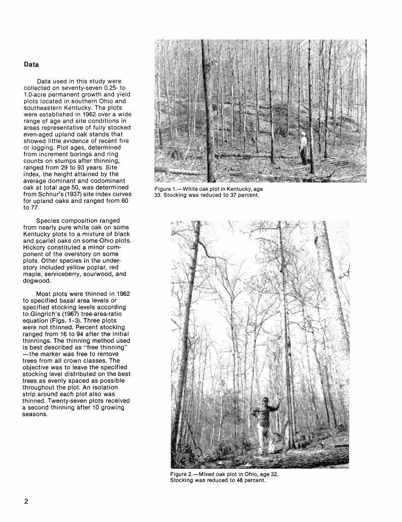
Data used in this study were collected on seventy-seven 0.25- to 1.0-acre permanent growth and yield plots located in southern Ohio and southeastern Kentucky. The plots were established in 1962 over a wide range of age and site conditions in areas representative of fully stocked even-aged upland oak stands that showed little evidence of recent fire or logging. Plot ages, determined from increment borings and ring counts on stumps after thinning, ranged from 29 to 93 years. Site index, the height attained by the averaae dominant and codominant oak a i total age 50, was determined Figure 1.-White oak plot in Kentucky, age from Schnur's (1937) site index curves 33. Stocking was reduced to 37 percent. for upland oaks and ranged from 60 to 77.

Species composit ion ranged from nearly pure white oak on some Kentucky plots to a mixture of black and scarlet oaks on some Ohio plots. Hickory constituted a minor com- ponent of the overstory on some plots. Other species in the under- story included yellow poplar, red maple, serviceberry, sourwood, and dogwood.

Most plots were thinned in 1962 to specified basal area levels or specified stocking levels according to Gingrich's (1967) tree-area-ratio equation (Figs. 1-3). Three plots were not thinned. Percent stocking ranged from 16 to 94 after the initial thinnings. The thinning method used is best described as "free thinning" -the marker was free to remove trees from all crown classes. The objective was to leave the specified stocking level distributed on the best trees as evenly spaced as possible throughout the plot. An isolation strip around each plot also was thinned. Twenty-seven plots received a second thinning after 10 growing seasons.

Figure 2.-Mixed oak plot in Ohio, age 32. Stocking was reduced to 48 percent.

Methods and Results

Model Development

Figure 3.-White oak plot in Kentucky, age 77. Stocking was reduced to 58 percent.

Every tree larger than 2.5 inches dbh was numbered and its species identified in 1962. Successive dbh measurements were recorded in 1962,1967,1972, and 1977. Growth statistics for the three 5-year periods were derived from these measure- ments. Only those trees larger than 2.5 inches dbh in 1962 were analyzed. lngrowth was excluded from the analysis because it is just now be- ginning to influence the growth of trees in the overstory. All trees used

The individual-tree diameter growth model was developed within limitations imposed by the data. A distance-independent model was developed because stem maps were not available for most plots. Stem maps prepared at the present time would not be useful because many trees have died or have been subse- quently thinned since the initial measurements. Dbh was the only variable recorded for each tree. Other variables such as crown ratio or crown class might have been useful for explaining variations in tree growth, but were not measured. Individual-tree growth, therefore, was modeled as a function of tree dbh and stand (plot) attributes. A major advantage of the resulting distance-independent model over distance-dependent models is that it allows for faster computing during execution, permitting rapid testing of many alternative management hy- potheses (Munro 1974).

The underlying assumption for using the diameter growth model developed in this study is that the user has access to a tree list for the stand. A tree list usually can be obtained by sampling the specific stand of interest. Species and dbh

in the analysis were appropriately should be rwmrded for each tree summed to obtain plot characteris- sampled. tics such as percent stocking, mean stand diameter, and basal area per acre. However, growth-model param- eters were fitted only to those trees of the five major commercial oak species: white, black, scarlet, chest- nut, and northern red. These five species constituted 84 percent of the 9,455 trees larger than 2.5 inches dbh after thinning in 1962.

Mean Model

The basic growth model proposed for development has the form:

where

BAG5YR,, = 5-year basal-area growth (ft2) for the jth tree in the ith stand,

DBHij = DBH (inches) of the jth tree in the ith stand, Sli = site index of the ith stand, - D, = mean stand diameter (quadratic mean) of the

ith stand, computed from trees larger than 2.5 inches dbh in the original tree list,

Psi = percent stocking of the ith stand, summed over trees larger than 2.5 inches dbh in the orig- inal tree list with Gingrich's (1967) stocking equation: PSij = - .005066 + .016977 DBHij + .003168 (DBHiJ2

I used basal-area growth as the dependent variable rather than diam- eter growth because visual relation- ships between variables are easier to detect when observing scatter plots of the data if basal-area rates are used. West (1980) found that the correlation between basal-area i ncre- ment and initial diameter was greater than that between diameter increment and initial diameter. However, the precision of estimates of future diameters were the same whether basal-area or d iameter-i ncrement equations were used.

The independent variables in- cluded in the model were limited to those previously found to have a significant effect on tree diameter growth for oaks (Dale 1975). Much of the variation in tree growth can be explained with initial tree size (DBH). The other variables reflect those stand attributes that most affect

tree growth: site index reflects site productivity, mean stand diameter reflects the size of the trees in the stand, and percent stocking reflects the degree of "crowding" in the stand. Stand age could be used in place of mean stand diameter, but it is determined with less reliability than mean stand diameter, which is calculated from the tree list. DBH and percent stocking also are ob- tained from the tree list. Site index can be readily determined in the field.

It is important to realize that other models may have performed as well as the hypothesized model. For example, another excellent combina- tion of independent variables would be dbh, number of stems per acre, and basal area per acre. However, since the proposed model performed well, no other models were explored because of the time and costs involved with model development.

A two-stage model building pro- cedure was used to develop the mean growth model. BAG5YR was first modeled as a function of DBH for each stand (plot). The parameters from these models were lhen mod- eled as a function of SI, D, and PS.

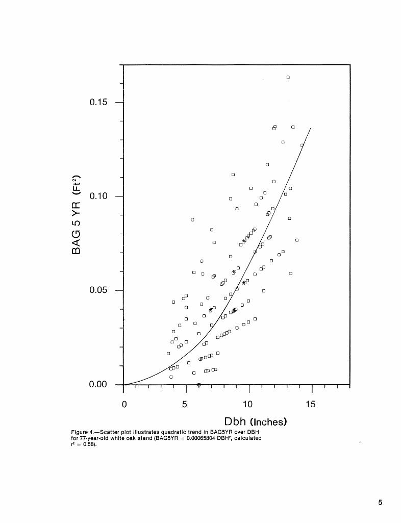
First-stage.-Investigation of scatter plots of BAG5YR on DBH (Fig. 4) suggests the development of the following first-stage model for each stand:

where /3,i, P2i, j33i are parameters to be estimated for the ith stand. The equa- tion is forced through the origin to prevent negative growth predictions. Given this condition, stepwise regres- sion procedures revealed that the (DBHij)2 term was the most significant variable for 75 percent of the plots. The added effect of the other two terms usually was not significant. The first-stage model, therefore, was simplified to the following form:

where bi is the sample estimate of the true parameter, pi, in the ith stand. In other words, BAG5YR has a quadratic trend over DBH, i.e., the 5-year basal-area growth of a tree is linearly related to the initial basal area of the tree. Ordinary least- squares analyses were performed to obtain unbiased estimates of the p's. Some plots displayed heteroge- neous variance about the regression line, which indicated that weighted regression techniques would be re- quired to obtain minimum-variance estimates of the 0's. However, ordi- nary least-squares estimates were considered satisfactory for the first stage of the modeling procedure because of the difficulty in deter- mining proper weights for each plot. The calculated rZ for equation (3) on most plots was about 0.70.'

'Calculated r2 = 1 - Z(yi - jri)2/~(yi - v)2

Dbh (Inches) Figure 4.-Scatter plot illustrates quadratic trend in BAGSYR over DBH for 77-year-old white oak stand (BAG5YR = 0.00065804 DBH2, calculated r2 = 0.58).

Since the data set contained few trees larger than 18 inches dbh, I was somewhat hesitant about accepting equation (3) as the first- stage model because the predicted 5-year basal-area growth can be very large for big trees due to the quad- ratic nature of the equation. One approach would be to limit model applications to the range of the data. However, growth predictions may be necessary in stands that contain very large trees. Therefore, an independent sample of individual tree growth rates for large trees was made in stands in southern Ohio. Several older, even-aged, mixed oak stands that contained many trees larger than 20 inches were sampled. Increment borings were used to determine past growth rates. Scatter plots of the past growth rates re- vealed no reason to reject equation (3) for very large trees (Fig. 5).

Scatter plots of all data revealed that equation (3) does not need to be adjusted for different oak species (Fig. 6). Tree size (DBH) accounts for most of the species effect on tree growth. In other words, big trees grow faster-regardless of species. Trees in the black oak group (black, scarlet, and northern red) usually are larger, hence faster growers, than white and chestnut oaks in a given stand (see stand tables in Schnur 1937, and Figure 6). Since this differ- entiation in tree size between species begins at an early age, growth models for very young stands would have to allow for different growth rates for different species. The growth models developed in this study should be applied only to stands where the size differentiation has already occurred -stands at least 30 years old.

A total of 231 8's were fitted- one for each of the three 5-year growth periods for the 77 plots. Correlations between growth rates for the three growth periods on a given plot were not considered during the construction of the mean model. They were, however, con- sidered during development of the random model. The next step in deveIopingJhe mean model was to- model the p's as a function of SI, D, and PS.

D bh (Inches) Figure 5.-Scatter plot illustrates quadratic trend in BAG5YR over DBH for 110-year-old stand, site index 75, that contained many large trees (BAG5YR = 0.00043849 DBH2, calculated r2 = 0.77).

Second-stage.-The value of is indicative of the basal-area growth for a g i v ~ n size tree. Scatter plots of the 291 3's revealed, as expected, that p increases as percent stocking is decreased. However, this increase is not as large for stands with larger mean stand diameters. TQe scatter piots also indicated that 0 increased on better sites.

The j ' s were best estimated with the following nonlinear equation:

where are sample estimates of the true parameters, ?,-y,, and EXP is the base of the natural log- arithms. After logarithmic transfor- mation, model parameters were estimated with a general linear model computer program:

The calculated r2 value was 0.76. Pre- dicted p's for site index 70 are shown in Figure 7.

Dbh (Inches) Figure 6.-Scatter plot ~l_f BAG5YR over DBH for all trees in the following category: SI < 65,10 < D < 15, and 40 < PS < 60. White oak and chestnut oak = 1; black, scarlet, and northern red = 2. Many code 1's were plotted first; note how code 2 overlaps code 1.

MEAN STAND DIAMETER (D) Figure 7.-Predicted j ' s for the equation BAG5YR = 8 (DBH)2, site index 70.

Random Model

Predicted growth rates and residuals (actual BAG5YR-predicted BAG5YR) for all trees were calcu!ated using equation (5) to determine j3i in equation (3). The overall calculated r2 value was 0.66. Predicted growth rates for a range of stocking and mean stand diameter conditions are shown in Figure 8 for site index 70.

The mean model, as discussed later, predicts individual-tree growth very well on the average. However, the quadratic nature of equation (3) does not allow trees within a given stand to change positions. Big trees always will be grown faster than smaller trees. Even though this feature of the mean model may not

Percent Stocking

- 5 inches --I0 inches

be serious regarding overall growth predictions, it is not realistic because trees do change positions. Methodol- ogy developed by Dale (1975) expands on the mean model by the use of a random growth component and a bivariate normal distribution between successive growth periods to allow trees to change positions.

Data plotted in this study sup- ported Dale's initial conclusion: (1) BAG5YR was distributed sym- metrically within most given size (dbh) classes and could be readily described with a standardized normal distribution, and (2) the distribution was somewhat skewed (positive) for smaller size classes, but not enough to prohibit use of the bivariate normal methodology. Therefore, the distri bu- tion of BAG5YR for a given growth period and size of tree can be defined if its mean and variance are known. The mean BAG5YR for a given tree size can be estimated with the mean model-equations (3) and (5). A gen- eral linear model computer program was used to develop an equation that predicts the standard deviation for a given tree size. The data were first divided into DBH, SI, D, and PS classes, and the standard deviation of BAGSYR was calculated for each class. The resulting regression equa- tion used to estimate the standard deviation for a given tree size, iiij,

had-a calculated r2 value equal to 0.67. SI, D, and PS did not significantly reduce the variation so they were not included in the model. Equation (6) is plotted in Figure 9.

4 8 12 16 20 Individual-tree growth for a given period can be randomly estimated with equations (3), (5), and (6) in the

Dbh (Inches) following manner: (1) generate a Figure 8.-Predicted 5-year basal-area growth rates (BAGSYR) for site random number, Z, from a normal index 70. distribution with mean = 0 and

variance = 1, and (2) recognizing that Z = (X - p)la, convert Z to the predicted basal-area growth for the 5-year period (Xii):

for k = 2 through n successive growth periods of interest. The quantity 6 represents the correlation between basal area growth for successive growth periods for a given dbh class. Extensive plotting of the data and regression analyses revealed that variations in fii could not be explained with SI, D l or PS. Values of 8 did not differ significantly between succes- sive growth periods either. An overall mean value of 0.632 was therefore used for 6.

The standard deviation, (Sij)k, about the conditional mean growth, (Yij),, in equation (8) is

The value of predicted growth for the first growth period, (Xij),, is deter- mined by random selection as in equation (7). The value of (Xij), for k > 1 is determined by first generating a random number, Z, from a normal distribution with mean = 0 and vari- ance = 1, then using (8) and (9) to convert Z to the predicted basal area growth:

The random-selection component in the random model allows trees to change position. However, inspection of equation (8) reveals the desirable feature of the bivariate normal ap- proach-the probability is high that fast-growing trees will remain fast growers and slow growers will remain slow growers.

In other words, the predicted 5-year basal-area growth for an indi- vidual tree is randomly selected from the distribution of basal-area growth about the mean for that size tree.

Randomly selecting the growth at successive growth periods would not be realistic unless the selection procedure were "tied together" in some fashion. If a bivariate normal

distribution between two successive growth periods for a given dbh class is assumed, the conditional mean of the predicted 5-year basal-area growth for the i-th tree in the j-th stand for the k-th growth period, (Yij),, given that the value of the growth from the previous period was (Xij)k-lt

Testing the Models

RandonrlKnown Model Test Procedures

The randomlknown model is identical to the random model except that the first 5-year growth, (X,,),, is known from past measurements. If (X,,), is known rather than randomly selected, position changes of trees in the stand are more likely to parallel actual changes. Unfortunately, actual 5-year growth records are seldom known in practice. However, when they are known, they should be used to the fullest extent.

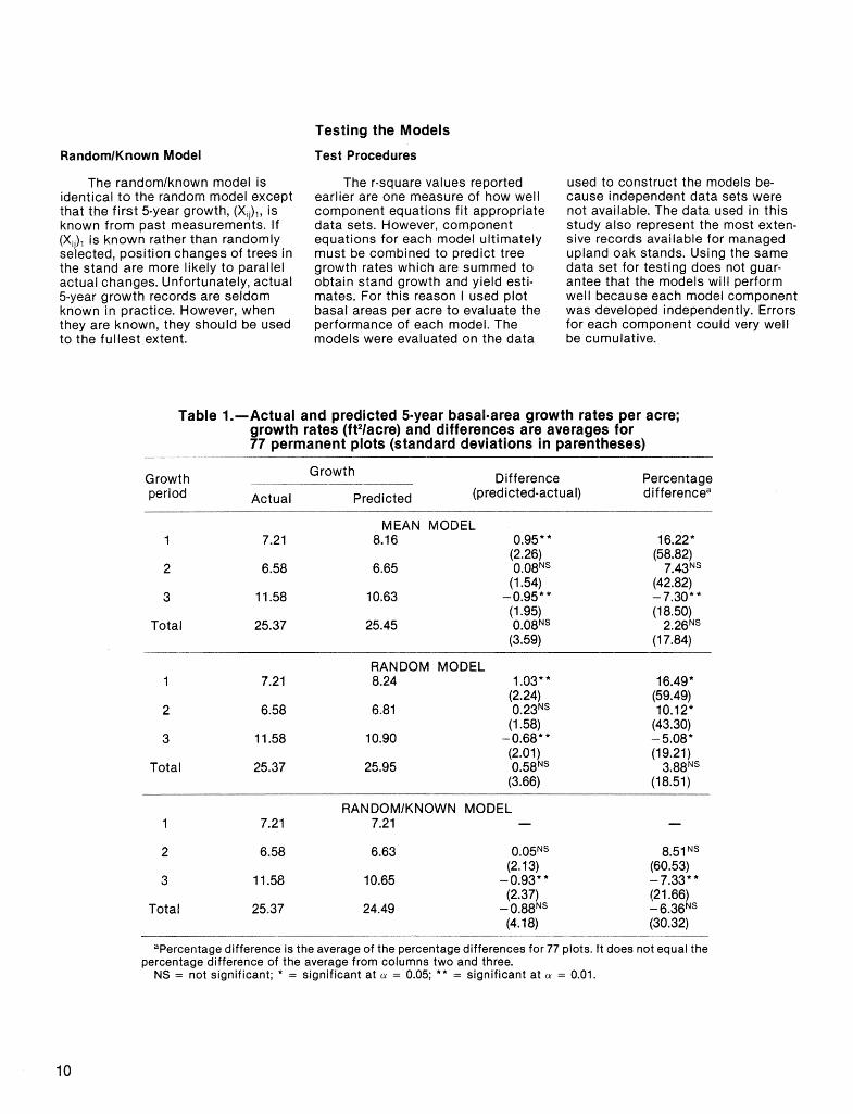
The r-square values reported earlier are one measure of how well component equations fit appropriate data sets. However, component equations for each model ultimately must be combined to predict tree growth rates which are summed to obtain stand growth and yield esti- mates. For this reason I used plot basal areas per acre to evaluate the performance of each model. The models were evaluated on the data

used to construct the models be- cause independent data sets were not available. The data used in this study also represent the most exten- sive records available for managed upland oak stands. Using the same data set for testing does not guar- antee that the models will perform well because each model component was developed independently. Errors for each component could very well be cumulative.

Table 1.-Actual and predicted 5-year basaimarea growth rates per acre; growth rates (ft2iacre) and differences are averages for 77 permanent plots (standard deviations in parentheses)

Growth period

Growth

Actual Predicted

Difference (predicted-actual)

Percentage differencea

MEAN MODEL 1 7.21 8.16 0.95* *

(2.26) 2 6.58 6.65 0.08NS

(1.54) 3 1 1.58 10.63 -0.95* *

(1.95) Total 25.37 25.45 0.08NS

(3.59)

RANDOM MODEL 1 7.21 8.24 1.03* *

(2.24) 2 6.58 6.81 0.23NS

(1 38) 3 1 1.58 10.90 -0.68**

(2.01) Total 25.37 25.95 0.58NS

(3.66)

RANDOMIKNOWN MODEL 1 7.21 7.21 -

2 6.58 6.63

3 11.58 10.65

Total 25.37 24.49

aPercentage difference is the average of the percentage differences for 77 plots. It does not equal the percentage difference of the average from columns two and three.

NS = not significant; * = significant at CY = 0.05; * * = significant at u = 0.01.

Test Results All trees larger than 2.5 inches

dbh in 1962 were used to test the growth models from 1962 to 1977. The equations developed in this study were applied to all trees in the tree list, regardless of species. Each plot was first "grown" for one 5-year period. Dead or cut trees were re- moved fro? the list and the stand attributes D and PS were then up- dated for input into the next 5-year growth projection. Three 5-year pro- jections were made with the mean and random models, but only two with the randomlknown model because the first growth period is given.

Since the mean model is deter- ministic, only one computer run was necessary to obtain the growth predictions. The random models, on the other hand, are stochastic, so growth predictions depend somewhat on the random numbers that are gen- erated. Ten computer runs were made for both the random and random1 known models, and the results were averaged to obtain the growth pre- dictions. Also, when the random and randomlknown models are used, the basal-area growth distribution for a given size class can include values less than zero. Since negative growth rates are not realistic, they were set equal to zero before the next 5-year growth prediction.

Average actual and predicted basal-area growth and yield values per acre are shown in Tables 1-2 for the 77 growth plots at each growth period. Since the growth rates are indicative of net growth, yield values in Table 2 can be determined by adding the growth rates in Table 1 except for the last 5-year period when cutting occurred.

Differences and percentage dif- ferences between actual and pre- dicted growth rates and yields were tested for significance (from zero) using t-tests at the end of each growth period, and also at the end of the entire growth projection. The

Table 2.-Actual and predicted basal-area yields per acre; yields (ft2/acre) and differences are averages for 77 permanent plats (standard deviations in parentheses)

Years after Basal arealacre initial Difference Percentage

measurement Actual Predicted (predicted-actual) differencea

MEAN MODEL 51 -41 51 -41 -

RANDOM MODEL 51.41 51.41 -

RANDOMIKNOWN MODEL 51.41 51.41 -

aPercentage difference is the average of percentage differences for 77 plots; it does not equal the percentage difference of the averages from columns two and three.

NS = not significant; * = significant at CY = 0.05; * * = significant at CY = 0.01.

percentage differences and their corresponding standard deviations provide perhaps the "clearest" view of model performance. For example, the percentage difference in growth for the mean model for the third growth period was -7.30 percent A 18.50 percent. These values indi- cate that, on the average, growth was estimated 7.30 percent low for the 77 plots, and that 67 percent (one standard deviation) of the predicted growth rates for given stands (plots) can be expected to fall between 25.8 percent low and 11.2 percent high.

Inspection of Tables 1-2 reveals an important fact about the growth projections-short-term projections can result in predicted values that are significantly different from actual values. In general, the predicted growth rates were too high for the first two growth periods and too low for the third 5-year period. However, total growth for the entire projection period was not significantly different from actual growth. Yields also were significantly different until the final growth period was completed.

On the basis of the data, I believe that the inability to make accurate short-term projections can be attrib- uted mostly to one unpredictable variable not included in growth mod- els-weather. The growth models were constructed with data from all three growth periods, so the weat her effects were essentially "averaged" into the model param- eters. The best we can do at the present time is to make growth predictions for "average" weather conditions, and be somewhat cau- tious in using growth models for very short-term projections.

Two other factors contribute to the differences between predicted and actual values: (1) all trees, re- gardless of species, were 'Qrown" with the models developed for oaks only, and (2) 27 of the 77 plots re- ceived a second thinning before the third growth period. The first factor probably is of little conse- quence because most of the trees were oaks. However, separate growth models for other species such as hickory and dogwood undoubtedly would increase the overall accuracy of the predictions. The effects of repeated thinnings in oak stands have not been investigated, but growth models that allow for effects of repeated thinnings also would undoubtedly increase overall accu- racy. The effects of repeated thinnings are beyond the scope of this paper -the assumption made here is that similar stands will respond the same, regardless of the number of thinnings.

Overall, all three growth models performed well. Growth was esti-

mated within 2 to 6 percent of the actual growth for the entire growth projection period, A 17 to 30 percent. Yields were within 1 percent, A 6 per- cent. The randomlknown model per- formed slightly worse than the other models even though the actual growth for the first period was included. This result occurred because of the weat her effects noted previously- predicted values only had two growth periods to "average" out.

Scatter plots of the residuals (predicted-actual) against SI, D, and PS revealed no biases for these variables. The only trend apparent in the plots of the residuals was that plots with low actual growth were overestimated, and those plots with high growth were underestimated.

Mean stand diameters also were calculated at the end of each growth period (Table 3). All three models projected the mean stand diameter well.

Table 3.-Actual and predicted mean stand diameters (D), based on averages for 77 permanent plots

Years since initial Acttual Mean Random Randomlknown

measurement D model model model

Inches 0 7.05 7.05 7.05 5 7.77 7.83 7.83

10 8.41 8.46 8.47 15 9.46 9.42 9.44

Discussion and Conclusions

The diameter growth models developed in this study are for use primarily as a component part of an individual-tree growth simulator for upland oak stands. A mortality model now being developed that removes trees from the tree list is required before the simulator can be used to project future growth and yield esti- mates. However, the diameter growth models can be functional at the present time if the user has access to mortality estimates and can dis- tribute the mortality throughout the tree list. Short projections (5 to 10 years) probably can be made if no mortality is assumed. Fractional portions of the 5-year projections can be made by linear interpolation.

Since all three growth models performed well, which model should be used? Obviously, the mean model must always be used because it is a component of both the random mod- els. However, the mean model is recommended only when the user does not have access to a high-speed computer. Equations (3) and (5) can be be easily programed in a programable calculator to obtain quick estimates of tree growth for office and field ap- plications. If a high-speed computer -almost essential for making projec- tions with individual-tree growth simulators-and the past 5 years' growth are available, then the random1 known model is recommended. If past growth is unknown, as i t usually is, then the random model should be used. Care should be exercised in selecting a reliable random number generator that is unbiased when using the random models.

Computer programs written in BASIC or FORTRAN for all three models are available from the author upon request. However, the user is encouraged to write his own pro- grams to ensure the desired program flexibility.

Test results in this study indi- cated that all three growth models predicted stand basal-area growth and yields satisfactorily. These results indicate how well the growth models perform as an aggregate of the individual-tree growth projec- tions. However, since we are also interested in the species and size class of individual trees, the distri- bution of the trees in the projected stand warrants investigation. Even though the distribution parameters were not modeled directly, we do not want the projected distribution to spread too much or too little. As an example, the distribution of trees for all three growth models after three 5-year projections was de-

termined for one plot (stand) only (Fig. 10). The site index on the plot was 70 and the mean stand diameter was 4.31 inches after thinning in 1962. Stocking was reduced to 53.04 percent in 1962, and a second thin- ning in 1972 lowered the percent stocking from 77.46 to 67.09 percent. Figure 10 shows that the projected distribution for the randomlknown model most closely approached that of the actual distribution in 1977. The mean and random model distri- butions were too high near the mean. Chi-square tests in which the numbers of trees by l-inch diameter classes were used were not significant for the randomlknown distribution, but were significant for the other two models.

RandomiKnown Model

D b h (Inches) Figure 10.-Actual and predicted diameter distributions for one stand (plot) in 1977 after 15 years' growth.

The order of the largest 15 trees on the plot in 1977 is shown in Ta- ble 4. The change in the rankings for the actual diameters from 1962 to 1977 demonstrates the dramatic changes that occur within a given stand. We are probably demanding too much of an individual-tree diam- eter growth model if we also expect the rankings to be predicted accu- rately. However, investigation of the resulting rankings can be informative. Spearman rank correlation tests revealed that only the randomlknown

model rankings were not significantly different from the actual rankings in 1977.

Distribution and rank tests are important indicators of model perfor- ance, but they are also costly and time consuming. Since the inclusion of the mortality model also affects the distribution and rank of trees, extensive testing in these areas for all plots is better left until the com- plete individual-tree growth simulator is developed.

Table 4.-Actual and predicted ranks of largest 15 trees for one stand (plot) in 1977 after 15 years' growth

Actual Actual Actual Predicted rank in 1977

rank dbh rank 1962 1977 1977

Mean Random Randomlknown model model model

Literature Cited

Dale, M. E. Growth and yield predic- tions for upland oak stands 10 years after initial thinning. Res. Pap. N E-241. Upper Darby, PA: U.S. Department of Agriculture, Forest Service, Northeastern Forest Ex- periment Station; 1972. 21 p.

Dale, M. E. Individual tree growth and simulation of stand development of an 80-year old white oak stand. In: Ek, A. R.; Balsinger, J. U.; Prominitz, L. C., eds. Forest modeling and inventory, selected papers from the 1973 and 1974 meetings of Midwest Mensurationists. Madison, WI: University of Wisconsin, School of Natural Resources; 1975: 49-63.

Gingrich, S. F. Measuring and evalu- ating stocking and stand density in upland hardwood forests in the central states. For. Sci. 13: 38-52; 1 967.

Hilt, D. E.; Dale, M. E. Height predic- tion equations for even-aged upland oak stands. Res. Pap. NE-493. Broomall, PA: U.S. Department of Agriculture, Forest Service, North- eastern Forest Experiment Station; 1982. 9 p.

Hilt, D. E. Taper-based system for estimating stem volumes of upland oaks. Res. Pap. NE-458. Broomall, PA: U.S. Department of Agriculture, F ~ r e s t Service, Northeastern Forest Experiment Station; 1980. 12 p.

Munro, D. D. Forest growth models- a prognosis. In: Growth models for tree and stand simulation. Res. Note 30. Stockholm, Sweden: Royal College, Department of Forestry; 1974: 7-21.

Schnur, L. G. Yield, stand, and volume tables for even-aged upland oak forests. Tech. Bull. 560. Washing- ton, DC: U.S. Department of Agri- culture; 1937. 87 p.

West, P. W. Use of diameter incre- ment and basal area increment in tree growth studies. Can. J. For. Res. 10: 71 -77; 1980.

fr U.S. GOVERNMENT PRINTING OFFICE: 1983-605-024117

Hilt, Donald E. Individual tree diameter growth model for managed, even-aged, upland oak stands. Res. Pap. NE-533. Broomall, PA: U.S. Department of Agriculture, Forest Service, Northeastern Forest Experiment Station; 1983. 15 p.

A distance-independent, individual-tree diameter growth model was developed for managed, even-aged, upland oak stands. The 5-year basal-area growth of individual trees is first modeled as a function of dbh squared for given stands. Parameters from these models are then modeled as a function of mean stand diameter, percent stocking of the stand, and site index. A stochastic option for the overall model also was developed. Tests on data from managed stands revealed that the model performed well.

Keywords: Distance-independent; stochastic; thinning

Headquarters of the Northeastern Forest Experiment Station are in Broomall, Pa. Field laboratories are maintained at:

Amherst, Massachusetts, in cooperation with the University of Massachusetts. Berea, Kentucky, in cooperation with Berea College. Burlington, Vermont, in cooperation with the University of Vermont. Delaware, Ohio. Durham, New Hampshire, in cooperation with the University of New Hampshire. Hamden, Connecticut, in cooperation with Yale University.

@ Morgantown, West Virginia, in cooperation with West Virginia University, Morgantown. Orono, Maine, in cooperation with the University of Maine, Orono. Parsons, West Virginia. Princeton, West Virginia. Syracuse, New York, in cooperation with the State University of New York College of Environmental Sciences and Forestry at Syracuse University, Syracuse.

6 University Park, Pennsylvania, in cooperation with the Pennsylvania State University. Warren, Pennsylvania.