44
Inference for parameters of interest after lasso model selection David M. Drukker Executive Director of Econometrics Stata Stata Conference 11-12 July 2019

Inference for parameters of interest after lasso
model selection
David M. Drukker
Executive Director of EconometricsStata
Stata Conference11-12 July 2019

Outline
Talk about methods for causal inference about some coefficientsin a high-dimensional model after using lasso for model selection
What are high-dimensional models?
What are some of the trade offs involved?
What are some of the assumptions involved?
1 / 40

High-dimensional models include too many potential covariatesfor a given sample size
I have an extract of the data Sunyer et al. (2017) used toestimate the effect air pollution on the response time of primaryschool children
htime i = no2iγ + xiβ + εi
htime measure of the response time on test of child i (hit time)no2 measure of the polution level in the school of child ixi vector of control variables that might need to be included
There are 252 controls in x, but I only have 1,084 observations
I cannot reliably estimate γ if I include all 252 controls
2 / 40

Potential solutions
htime i = no2iγ + xiβ + εi
I am willing to believe that the number of controls that I need toinclude is small relative to the sample size
This is known as a sparsity assumption
3 / 40
Potential solutions
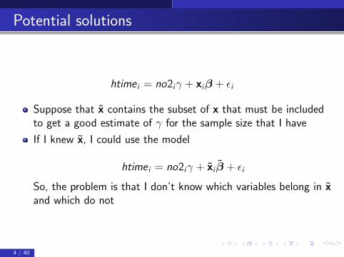
htime i = no2iγ + xiβ + εi
Suppose that x contains the subset of x that must be includedto get a good estimate of γ for the sample size that I have
If I knew x, I could use the model
htime i = no2iγ + xi β + εi
So, the problem is that I don’t know which variables belong in xand which do not
4 / 40
Potential solutions
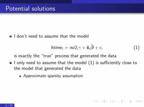
I don’t need to assume that the model
htime i = no2iγ + xi β + εi (1)
is exactly the “true” process that generated the data
I only need to assume that the model (1) is sufficiently close tothe model that generated the data
Approximate sparsity assumption
5 / 40

htime i = no2iγ + xi β + εi
Now I have a covariate-selection problem
Which of the controls in x belong in x ?
A covariate-selection method can be data-based or notdata-based
Using theory to decide which variables go into x is anon-data-based method
Live with/assume away the bias due to choosing wrong xNo variation of selected model in repeated samples
6 / 40

Many researchers want to use data-based methods ormachine-learning methods to perform the covariate selection
These methods should be able to remove the bias (possibly)arising from non-data-based selection of x
Some post-covariate-selection estimators provide reliableinference for the few parameters of interest
Some do not
7 / 40

A naive approach
A “naive” solution is :
1 Always include the covariates of interest2 Use covariate-selection to obtain an estimate of which
covariates are in xDenote estimate by xhat
3 Use estimate xhat as if it contained the covariates in xregress htime no2 xhat
8 / 40

Why naive approach fails
Unfortunately, naive estimators that use the selected covariatesas if they were x provide unreliable inference in repeated samples
Covariate-selection methods make too many mistakes inestimating x when some of the coefficients are small inmagnitudeHere is an example of small coefficient
A coefficient with a magnitude between 1 and 2 times thestandard error is small
If your model only approximates the functional form of the truemodel, there are approximation terms
The coefficients on some of the approximating terms are mostlikely small
9 / 40

Missing small-cofficient covariates matters
It might seem that not finding covariates with small coefficientsdoes not matter
But it doesMissing covariates with small coefficients even matters in simplemodels with a only few covariates
10 / 40

Here is an illustration of the problems with naive post-selectionestimators
Consider the linear model
y =x1 + s x2 + ε
where s is about about twice its standard error
Consider a naive estimator for the coefficent on x1 (whose valueis 1)
1 Regress y on x1 and x22 Use a Wald test to decide if the coefficient on x2 is significantly
different from 03 Regress y on{
x1 and x2 if the coefficient is significant
x1 if the coefficient is not significant
11 / 40

This naive estimator performs poorly in theory and in practice
In an illustrative Monte Carlo simulation, the naive estimator hasa rejection rate of 0.13 instead of 0.05
The theoretical distribution used for inference is a badapproximation to the actual distribution
05
1015
20
.9 .95 1 1.05 1.1b1_e
Actual distribution Theoretical distribution
12 / 40

Why the naive esimator performs poorly I
When some of the covariates have small coefficients, thedistribution of the covariate-selection method is not sufficientlyconcentrated on the set of covariates that best approximates theprocess that generated the data
Covariate-selection methods will frequently miss the covariateswith small coefficients causing ommitted variable bias
13 / 40
Why the naive esimator performs poorly II
The random inclusion or exclusion of these covariates causes thedistribution of the naive post-selection estimator to be notnormal and makes the usual large-sample theory approximationinvalid in theory and unreliable in finite samples
14 / 40

Beta-min condition
The beta-min condition was invented to rule-out the existence ofsmall coefficients in the model that best approximates theprocess that generated the data
Beta-min conditions are super restrictive and are widely viewedas not defensible
See Leeb and Potscher (2005); Leeb and Potscher (2006); Leeband Potscher (2008); and Potscher and Leeb (2009)See Belloni, Chernozhukov, and Hansen (2014a) and Belloni,Chernozhukov, and Hansen (2014b)
15 / 40
Partialing-out estimators
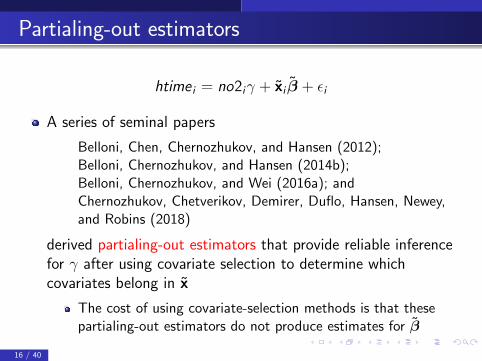
htime i = no2iγ + xi β + εi
A series of seminal papers
Belloni, Chen, Chernozhukov, and Hansen (2012);Belloni, Chernozhukov, and Hansen (2014b);Belloni, Chernozhukov, and Wei (2016a); andChernozhukov, Chetverikov, Demirer, Duflo, Hansen, Newey,and Robins (2018)
derived partialing-out estimators that provide reliable inferencefor γ after using covariate selection to determine whichcovariates belong in x
The cost of using covariate-selection methods is that thesepartialing-out estimators do not produce estimates for β
16 / 40

Recommendations
I am going to provide lots of details, but here are two take aways
1 If you have time, use the cross-fit partialing-out estimator
xporegress, xpologit, xpopoisson, xpoivregress
2 If the cross-fit estimator takes too long, use either thepartialing-out estimator
poregress, pologit, popoisson, poivregress
or the double-selection estimator
dsregress, dslogit, dspoisson
17 / 40
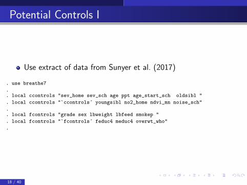
Potential Controls I
Use extract of data from Sunyer et al. (2017)
. use breathe7
.
. local ccontrols "sev_home sev_sch age ppt age_start_sch oldsibl "
. local ccontrols "`ccontrols´ youngsibl no2_home ndvi_mn noise_sch"
.
. local fcontrols "grade sex lbweight lbfeed smokep "
. local fcontrols "`fcontrols´ feduc4 meduc4 overwt_who"
.
18 / 40
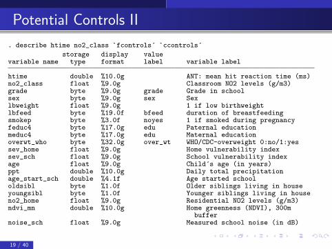
Potential Controls II
. describe htime no2_class `fcontrols´ `ccontrols´
storage display valuevariable name type format label variable label
htime double %10.0g ANT: mean hit reaction time (ms)no2_class float %9.0g Classroom NO2 levels (g/m3)grade byte %9.0g grade Grade in schoolsex byte %9.0g sex Sexlbweight float %9.0g 1 if low birthweightlbfeed byte %19.0f bfeed duration of breastfeedingsmokep byte %3.0f noyes 1 if smoked during pregnancyfeduc4 byte %17.0g edu Paternal educationmeduc4 byte %17.0g edu Maternal educationoverwt_who byte %32.0g over_wt WHO/CDC-overweight 0:no/1:yessev_home float %9.0g Home vulnerability indexsev_sch float %9.0g School vulnerability indexage float %9.0g Child´s age (in years)ppt double %10.0g Daily total precipitationage_start_sch double %4.1f Age started schoololdsibl byte %1.0f Older siblings living in houseyoungsibl byte %1.0f Younger siblings living in houseno2_home float %9.0g Residential NO2 levels (g/m3)ndvi_mn double %10.0g Home greenness (NDVI), 300m
buffernoise_sch float %9.0g Measured school noise (in dB)
19 / 40
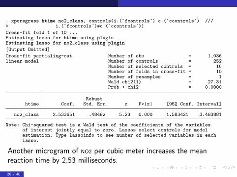
. xporegress htime no2_class, controls(i.(`fcontrols´) c.(`ccontrols´) ///> i.(`fcontrols´)#c.(`ccontrols´))
Cross-fit fold 1 of 10 ...Estimating lasso for htime using pluginEstimating lasso for no2_class using plugin
[Output Omitted]
Cross-fit partialing-out Number of obs = 1,036linear model Number of controls = 252
Number of selected controls = 16Number of folds in cross-fit = 10Number of resamples = 1Wald chi2(1) = 27.31Prob > chi2 = 0.0000
Robusthtime Coef. Std. Err. z P>|z| [95% Conf. Interval]
no2_class 2.533651 .48482 5.23 0.000 1.583421 3.483881
Note: Chi-squared test is a Wald test of the coefficients of the variablesof interest jointly equal to zero. Lassos select controls for modelestimation. Type lassoinfo to see number of selected variables in eachlasso.
Another microgram of NO2 per cubic meter increases the meanreaction time by 2.53 milliseconds.
20 / 40
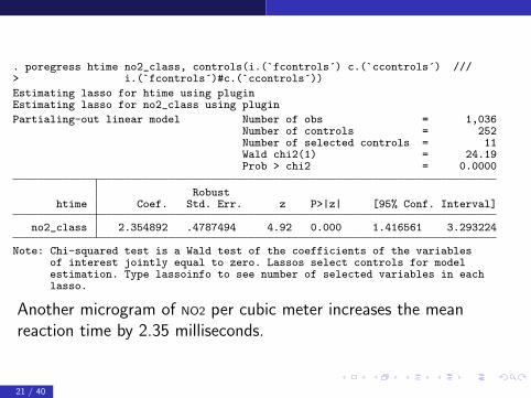
. poregress htime no2_class, controls(i.(`fcontrols´) c.(`ccontrols´) ///> i.(`fcontrols´)#c.(`ccontrols´))
Estimating lasso for htime using pluginEstimating lasso for no2_class using plugin
Partialing-out linear model Number of obs = 1,036Number of controls = 252Number of selected controls = 11Wald chi2(1) = 24.19Prob > chi2 = 0.0000
Robusthtime Coef. Std. Err. z P>|z| [95% Conf. Interval]
no2_class 2.354892 .4787494 4.92 0.000 1.416561 3.293224
Note: Chi-squared test is a Wald test of the coefficients of the variablesof interest jointly equal to zero. Lassos select controls for modelestimation. Type lassoinfo to see number of selected variables in eachlasso.
Another microgram of NO2 per cubic meter increases the meanreaction time by 2.35 milliseconds.
21 / 40
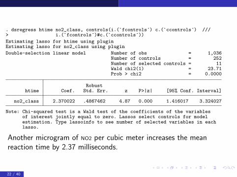
. dsregress htime no2_class, controls(i.(`fcontrols´) c.(`ccontrols´) ///> i.(`fcontrols´)#c.(`ccontrols´))
Estimating lasso for htime using pluginEstimating lasso for no2_class using plugin
Double-selection linear model Number of obs = 1,036Number of controls = 252Number of selected controls = 11Wald chi2(1) = 23.71Prob > chi2 = 0.0000
Robusthtime Coef. Std. Err. z P>|z| [95% Conf. Interval]
no2_class 2.370022 .4867462 4.87 0.000 1.416017 3.324027
Note: Chi-squared test is a Wald test of the coefficients of the variablesof interest jointly equal to zero. Lassos select controls for modelestimation. Type lassoinfo to see number of selected variables in eachlasso.
Another microgram of NO2 per cubic meter increases the meanreaction time by 2.37 milliseconds.
22 / 40

Estimators
Estimators use the least absolute shrinkage and selectionoperator (lasso) to perform covariate-selection
For now just think of lasso as covariate-selection method thatworks when the number of potential covariates is large
The number of potential covariates p can be greater than thenumber of observations N
23 / 40

Partialing-out estimator for linear model
Consider model
y = dγ + xβ + ε
For simplicity, d is a single variable, all methods handle multiplevariables
I discuss a linear model
Nonlinear models have similar methods that involve more details
24 / 40

PO estimator for linear model (I)
y = dγ + xβ + ε
1 Use a lasso of y on x to select covariates xy that predict y
2 Regress y on xy and let y be residuals from this regression
3 Use a lasso of d on x to select covariates xd that predict d
4 Regress d on xd and let d be residuals from this regression
5 Regress y on d to get estimate and standard error for γ
Only the coefficient on d is estimated
Not estimating β can be viewed as the cost of getting reliableestimates of γ that are robust to the mistakes thatmodel-selection techniques make
25 / 40
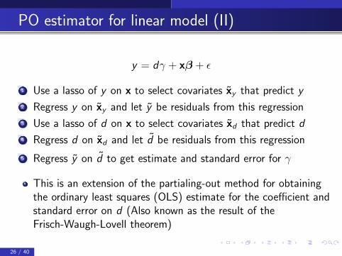
PO estimator for linear model (II)
y = dγ + xβ + ε
1 Use a lasso of y on x to select covariates xy that predict y
2 Regress y on xy and let y be residuals from this regression
3 Use a lasso of d on x to select covariates xd that predict d
4 Regress d on xd and let d be residuals from this regression
5 Regress y on d to get estimate and standard error for γ
This is an extension of the partialing-out method for obtainingthe ordinary least squares (OLS) estimate for the coefficient andstandard error on d (Also known as the result of theFrisch-Waugh-Lovell theorem)
26 / 40

y = dγ + xβ + ε
1 Use a lasso of y on x to select covariates xy that predict y2 Regress y on xy and let y be residuals from this regression3 Use a lasso of d on x to select covariates xd that predict d4 Regress d on xd and let d be residuals from this regression
5 Regress y on d to get estimate and standard error for γ
Heuristically, the moment conditions used in step 5 are unrelatedto the selected covariates
Formally, the moments conditions used in step 5 have beenorthogonalized, or “immunized” to small mistakes in covariateselection
Chernozhukov, Hansen, and Spindler (2015a); andChernozhukov, Hansen, and Spindler (2015b)
27 / 40

Double-selection estimators
y = dγ + xβ + ε
Double-selection estimators extend the PO approach
1 Use a lasso of y on x to select covariates xy that predict y
2 Use a lasso of d on x to select covariates xd that predict d
3 Let xu be the union of the covariates in xy and xd4 Regress y on d and xu
The estimation results for the coefficient on d are the estimationresults for γ
28 / 40

Cross-fitting / double-machine-learning PO
Cross-fitting is also known as double maching learning (DML)
It uses split-sample techniques on PO estimators
to weaken the sparsity conditionto get better finite sample performance
Split-sample techniques further reduce the impact of covariateselection on the estimator for γ
It’s the combination of a sample-splitting technique with a POestimator that gives cross-fit PO estimators their reliability
29 / 40
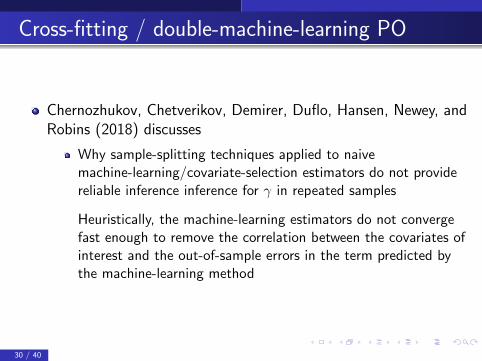
Cross-fitting / double-machine-learning PO
Chernozhukov, Chetverikov, Demirer, Duflo, Hansen, Newey, andRobins (2018) discusses
Why sample-splitting techniques applied to naivemachine-learning/covariate-selection estimators do not providereliable inference inference for γ in repeated samples
Heuristically, the machine-learning estimators do not convergefast enough to remove the correlation between the covariates ofinterest and the out-of-sample errors in the term predicted bythe machine-learning method
30 / 40

Cross-fitting / double-machine-learning PO
Chernozhukov, Chetverikov, Demirer, Duflo, Hansen, Newey, andRobins (2018) discusses
PO estimators simplify the problem and their distributionsdepend on the correlation between partialed-out covariate ofinterest and the errors in the term predicted by themachine-learning method
Naive estimator depends correlation between the covariate ofinterest and the errors in the term predicted by themachine-learning method
Sample-splitting gets better properties by depending on theout-of-sample correlation between partialed-out covariate ofinterest and the errors in the term predicted by themachine-learning method instead of the in-sample correlation
31 / 40

1 Split data into samples A and B2 Using the data in sample A
1 Use a lasso of y on x to select covariates xy that predict y2 Regress y on xy and let βA be the estimated coefficients3 Use a lasso of d on x to select covariates xd that predict d4 Regress d on xd and let δA be the estimated coefficients
3 Using the data in sample B1 Fill in the residuals for y = y − xy βA
2 Fill in the residuals for d = d − xd δA4 Using the data in sample B
1 Use a lasso of y on x to select covariates xy that predict y2 Regress y on xy and let βB be the estimated coefficients3 Use a lasso of d on x to select covariates xd that predict d4 Regress d on xd and let δB be the estimated coefficients
5 Using the data in sample A1 Fill in the residuals for y = y − xy βB
2 Fill in the residuals for d = d − xd δB6 Regress y on d to get estimates for γ
32 / 40

What’s a lasso?
β = arg minβ
{1/n
n∑i=1
(yi − xiβ′) + λ
k∑j=1
ωj |βj |
}
For λ ∈ (0, λmax) some of the estimated coefficients are exactlyzero and some of them are not zero.
This is how the lasso works as a covariate-selection method
Covariates with estimated coefficients of zero are excludedCovariates with estimated coefficients that not zero are included
33 / 40

Choosing λ
You must choose λ before you use the lasso to perform covariateselection
We talk about choosing λ, but really we are choosing λ andcoefficient penalty loadings ωj (j ∈ {1, . . . , p})The value of λ determines which covariates will be included andwhich will be excluded
The value of λ determines which covariates will have estimatedcoefficients that are not zero and which covariates will haveestimated coefficients that are zero
34 / 40

Choosing λ
We want a λ that selects covariates x so that E[y |d , x] issufficiently close to the true conditional mean
Approximate sparsity allows the E[y |d , x] to differ from the trueconditional mean, but this approximation error can’t be toolarge
We don’t want to select covariates that do not contribute toapproximating the conditional mean
Including too many extra covariates can cause out{PO,DS,XPO} estimator to performly poorly(Including too many extra covariates slows the convergence rateof the {PO,DS,XPO} estimator)
35 / 40

Choosing λ
Three methods for selecting λ are
1 Plug-in estimators
These estimators are the default in the PO, DS, and XPOcommands
2 Cross-validation3 The adaptive lasso
36 / 40

Plug-in based lasso
Plug-in estimators find the value of the λ that is large enough todominate the estimation noise
In practice, the plug-in-based lasso tends to include theimportant covariates and it is really good at not includingcovariates that do not belong in the model
see Belloni, Chernozhukov, and Wei (2016b); Belloni, Chen,Chernozhukov, and Hansen (2012); and Bickel et al. (2009)
37 / 40

Cross-validated lasso
Cross-valdiation (CV) finds the β that minimizes theout-of-sample prediction error
CV is widely used for prediction lasso, but it is usually not thebest method when using lasso as a covariate-selection method ina PO, XPO, or DS estimator
CV tends to choose a λ that causes lasso to include variableswhose coefficients are zero in the model that best approximatesthe true data generating processThis over-selection tendency can cause a CV-based {PO,DS,XPO} estimator to have poor coverage properties
(Although the XPO estimators are more robust to this problemthan PO and DS estimators)
38 / 40

Adaptive lasso
The adaptive lasso tends to include more zero-coefficientcovariates than a plug-in based lasso and fewer than across-validated lasso
39 / 40
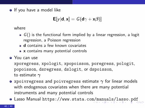
If you have a model like
E[y |d, x] = G (dγ + xβ)]
where
G () is the functional form implied by a linear regression, a logitregression, a Poisson regressiond contains a few known covariatesx contains many potential controls
You can usexporegress, xpologit, xpopoisson, poregress, pologit,popoisson, dsregress, dslogit, or dspoisson,to estimate γ
xpoivregress and poivregress estimate γ for linear modelswith endogenous covariates when there are many potentialinstruments and many potential controls
Lasso Manual https://www.stata.com/manuals/lasso.pdf
40 / 40

References
Belloni, A., D. Chen, V. Chernozhukov, and C. Hansen. 2012. Sparsemodels and methods for optimal instruments with an application toeminent domain. Econometrica 80(6): 2369–2429.
Belloni, A., V. Chernozhukov, and C. Hansen. 2014a.High-dimensional methods and inference on structural andtreatment effects. Journal of Economic Perspectives 28(2): 29–50.
. 2014b. Inference on treatment effects after selection amonghigh-dimensional controls. The Review of Economic Studies 81(2):608–650.
Belloni, A., V. Chernozhukov, and Y. Wei. 2016a. Post-selectioninference for generalized linear models with many controls. Journalof Business & Economic Statistics 34(4): 606–619.
. 2016b. Post-Selection Inference for Generalized Linear ModelsWith Many Controls. Journal of Business & Economic Statistics34(4): 606–619.
Bickel, P. J., Y. Ritov, and A. B. Tsybakov. 2009. Simultaneous40 / 40

References
analysis of Lasso and Dantzig selector. The Annals of Statistics37(4): 1705–1732.
Chernozhukov, V., D. Chetverikov, M. Demirer, E. Duflo, C. Hansen,W. Newey, and J. Robins. 2018. Double/debiased machine learningfor treatment and structural parameters. The EconometricsJournal 21(1): C1–C68.
Chernozhukov, V., C. Hansen, and M. Spindler. 2015a.Post-Selection and Post-Regularization Inference in Linear Modelswith Many Controls and Instruments. American Economic Review105(5): 486–90. URL http:
//www.aeaweb.org/articles?id=10.1257/aer.p20151022.
. 2015b. Valid Post-Selection and Post-RegularizationInference: An Elementary, General Approach. Annual Review ofEconomics 7(1): 649–688.
Leeb, H., and B. M. Potscher. 2005. Model Selection and Inference:Facts and Fiction. Econometric Theory 21: 21–59.
40 / 40

Bibliography
. 2006. Can one estimate the conditional distribution ofpost-model-selection estimators? The Annals of Statistics 34(5):2554–2591.
. 2008. Sparse estimators and the oracle property, or the returnof Hodges estimator. Journal of Econometrics 142(1): 201–211.
Potscher, B. M., and H. Leeb. 2009. On the distribution of penalizedmaximum likelihood estimators: The LASSO, SCAD, andthresholding. Journal of Multivariate Analysis 100(9): 2065–2082.
Sunyer, J., E. Suades-Gonzlez, R. Garca-Esteban, I. Rivas, J. Pujol,M. Alvarez-Pedrerol, J. Forns, X. Querol, and X. Basagaa. 2017.Traffic-related Air Pollution and Attention in Primary SchoolChildren: Short-term Association. Epidemiology 28(2): 181–189.
40 / 40


