Inflation, Demand for Liquidity, and Welfare - … · ation, Demand for Liquidity, and Welfare ......

Inflation, Demand for Liquidity, and Welfare

Shutao Cao Cesaire A. Meh Jose-Vıctor Rıos-Rull Yaz Terajima

Bank of Canada Bank of Canada University of Minnesota Bank of CanadaMpls Fed, CAERP

Sixty Years Since Baumol-Tobin: A Celebration Conference

New York University

Preliminary

September 26, 2012

The views expressed are those of the authors and not of the Bank of Canada, the

Federal Reserve Bank of Minneapolis or the Federal Reserve System.

Motivation

Inflation affects relative prices of holding different types of assets andhence welfare.

Most previous studies use representative-agent models and aggregateevidence to measure the cost.

I Dotsey and Ireland (1996), Lucas (2000), among others.

Heterogeneous behavior and micro evidence can be important.

Shutao Cao, Cesaire A. Meh, Jose-Vıctor Rıos-Rull, Yaz Terajima New York University

Inflation, Demand for Liquidity, and Welfare September 26, 2012 2/42

Motivation

Recent work on welfare cost of inflation take into accountheterogeneity.

I Welfare cost varies considerably across households: Mulligan and

Sala-i-Martin (2000), Doepke and Schneider (2006), Meh and Terajima (2008),

Erosa and Ventura (2002), Chiu and Molico (2008)

I Aggregate welfare effects can differ when heterogeneity is considered

Not much done in the literature:

I Money holding for transaction purpose varies with age.

This is important because

I Welfare cost of inflation will differ across age groups

I Potential nonlinear effects of inflation when aggregated



Other literature

Lucas (2000) points out an importance of using micro data toestimate the gains/costs of inflation.

Mulligan and Sala-i-Martin (2000) and Attanasio et al. (2002) usemicro data to estimate the welfare cost of inflation.

Dotsey and Ireland (1996) analyze a general equilibrium model ofmoney demand with an intermediation cost of credit transactiontechnology.

Erosa and Venture (2002) incorporates heterogeneity over householdincome.

Chui and Molico (2010) uses a search model of demand for money.

Heer and Maussner (2012) analyze the effects of inflation ondistributions of both income and wealth.

Heer et al. (2007) document that the money-age profile ishump-shaped and money is weakly correlated with income andwealth.

Ragot (2010) documents that the distribution of money acrosshouseholds is more similar to that of financial assets than ofconsumption.



What we do

1 Ask welfare implications of inflation by

I building an OLG model where money and credit are used fortransaction; and

I calibrating model to capture age, cohort and time effects onmoney-consumption ratios.

2 Document money-consumption ratios, i.e., liquidity demand formoney

I People are very different between ages and between social classes overmoney holdings and wealth

3 Use data to disentangle age, cohort and time effects



Findings

Money-consumption ratio is higher for older and poor households.

I 5 times higher for old households (aged 76-85) relative to that foryoung (aged 26-35)

I 2 times higher for poor households relative to that for rich households

These effects do not disappear once we control for cohort and timeeffects.

Age-specific transaction cost captures age profile of money holding.

Aggregate welfare effects when inflation ↑ from 1.92% to 10%,

I Aggregate consumption decreases by 0.83%.

Distributional effects are summarize as follows,

I To be added



Data: Two Household Surveys

Our main data sources are two household surveys (repeatedcross-section)

Canadian Financial Monitor (CFM), 1999-2010, by Ipsos Reid

I “money” holdings information available for all years

I consumption information available only for 2008-2010

Survey of Household Spending (SHS), 1999-2009, by StatisticsCanada

I no information on money holdings

I consumption information available for all years

Money: checking account and some savings accounts (fortransactions)

Consumption: durables (excluding housing), non-durables, and service



Data: Combining CFM and SHS

To separate out age, cohort and time effects, we need data onmoney-con ratios over a longer period than 2008-2010 from CFM.

Obtain a 11-year series by combining CFM and SHS, followingBethencourt and Rıos-Rull (2009):

1 From 2008-2010 CFM, calculate a joint distribution (in quintile) ofhouseholds over money and consumption.

2 For each year over 1999-2009, calculate average money holdings ofhouseholds in each quintile from CFM and average consumption ineach quintile from SHS.

3 Holding fixed the joint distribution from Step (1), assign the averagemoney holdings and consumption in the respective quintile in each yearover 1999-2009.

4 For each year and each consumption quintile, calculate averagemoney-consumption ratios over money quintile using the marginaldistribution from Step (1) as weights.



Data: Joint distribution of Money and Consumption

CFM 2008-2010 contain household-level information regarding moneyand consumption. Hence, we can construct a joint distribution ofhouseholds over money and consumption:

w.1 w.2 w.3 w.4 w.5

5th w51 w52 w53 w54 w55 w5.

Money 4th w41 w42 w43 w44 w45 w4.

Quintile 3rh w31 w32 w33 w34 w35 w3.

2nd w21 w22 w23 w24 w25 w2.

1st w11 w12 w13 w14 w15 w1.

1st 2nd 3rd 4th 5th Marginal

Consumption Distribution

Quintile

Marginal Dist.



Data: Joint distribution of Money and Consumption

For each year over the 1999-2007 period,

I CFM has information on money, {w1., ...,w5.}, andI we can calculate average money holdings in each quintile.

I SHS has information on consumption, {w.1, ...,w.5}, andI we can calculate average consumption in each quintile.

Use these information to approximate money-consumption ratios ineach consumption quintile.



Data: Combining CFM and SHS

Do this for six age groups:

I Aged 26-35, 36-45, 46-55, 56-65, 66-75 and 76-85.



Money-Consumption Ratio by Consumption

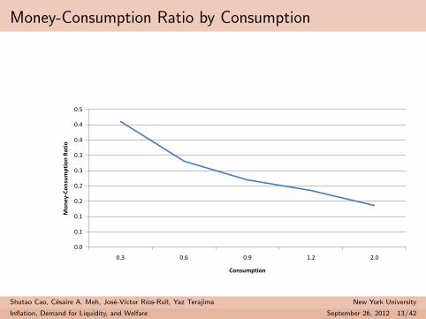
Money-consumption ratio declines as consumption increases.



Money-Consumption Ratio by Consumption

0.0

0.1

0.1

0.2

0.2

0.3

0.3

0.4

0.4

0.5

0.3 0.6 0.9 1.2 2.0

Mo

ne

y-C

on

sum

pti

on

Rat

io

Consumption



Money-Consumption Ratio by Consumption and Age

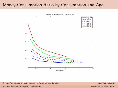
Money-consumption ratio rises with household age.



Money-Consumption Ratio by Consumption and Age

0.5 1 1.5 2 2.50

0.2

0.4

0.6

0.8

1

Consumption

Money−consumption ratio, CFM 2008−2010

age<3536−4546−5556−6566−7576−85



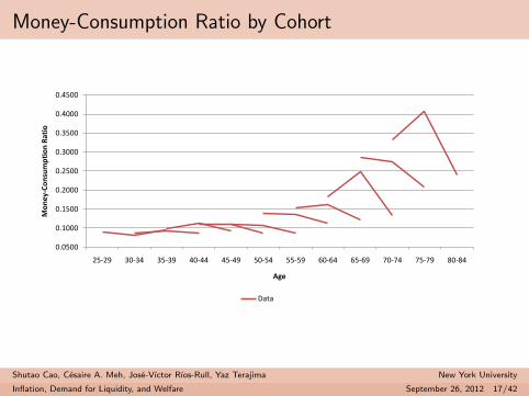
Money-Consumption Ratio by Cohort

Money-consumption ratio declines for newer cohorts.

I Older cohorts have higher money-consumption ratios givenconsumption.



Money-Consumption Ratio by Cohort

0.0500

0.1000

0.1500

0.2000

0.2500

0.3000

0.3500

0.4000

0.4500

25-29 30-34 35-39 40-44 45-49 50-54 55-59 60-64 65-69 70-74 75-79 80-84

Mo

ne

y-C

on

sum

pti

on

Rat

io

Age

Data



Money-Consumption Ratio Over Time

Aggregate money-consumption ratios change over time with themacroeconomic environment.



Money-Consumption Ratio Over Time

consumpreal moneyreal

1.20

1.30

1.40

1.50

1.60

1.70

1.80

1.90

2.00

1999 2000 2001 2002 2003 2004 2005 2006 2007 2008 2009

Ave

rage

Mo

ne

y-C

on

sum

pti

on

Rat

io

Year



Money and Consumption Over Time2004

2500

3000

3500

4000

4500

5000

5500

6000

6500

1999 2000 2001 2002 2003 2004 2005 2006 2007 2008 2009

$

Year

consumpreal moneyreal



Empirical Analysis on Money-Consumption Ratios by Age,Cohort and Time

It is difficult to separate out these three effects.

Our identification strategy and assumptions are:

I Three effects are independent

I Cohort effects are assumed to be exponential with respect to thedifferences in birth year (µ∆birth year/10)

I Time effects are time-specific (λtime)

I Age effects are age-specific (αage)

Estimate µ, λt and αi using annual data on money-consumptionratios from 1999 to 2009, with six 10-year age groups.



Estimation of cohort, time and age effects

Use the following moment conditions:

(mc

)1,1999

= α1

(mc

)1,2000

= α1µ1

10 λ2000 · · ·(

mc

)1,2009

= α1µλ2009(mc

)2,1999

= α21µ

(mc

)2,2000

= α21

µ1− 1

10λ2000 · · ·

(mc

)2,2009

= α2λ2009

......

...(mc

)i,1999

= αi1

µi−1

(mc

)i,2000

= αi1

µi− 1

10λ2000 · · ·

(mc

)i,2009

= αi1

µi−2 λ2009

......

...(mc

)I ,1999

= αI1

µI−1

(mc

)I ,2000

= αI1

µI− 1

10λ2000 · · ·

(mc

)J,2009

= αI1

µI−2 λ2009

This gives us I × 11 equations and I + 11 parameters.



Estimation of cohort, time and age effects

Additional assumptions we make are:

Cohort effects reduce the demand for money over time: µ ∈ (0, 1)



Estimation results

α1 α2 α3 α4 α5 α6 µ0.091 0.109 0.123 0.175 0.297 0.498 0.994

(0.001) (0.001) 0.002) (0.002) (0.003) (0.007) (0.864)

λ00 λ01 λ02 λ03 λ04 λ05 λ06 λ07 λ08 λ090.96 0.86 0.72 0.96 0.95 0.93 1.02 0.93 0.77 0.67

(0.014) (0.013) (0.013) (0.014) (0.015) (0.016) (0.015) (0.015) (0.013) (0.007)

λ99 ≡ 1 by normalization

Use the estimates to calibrate the following model.

For calibration, the averages over λ99 − λ04 and λ05 − λ09 are used asthe time effects since the model period is 10 years.



We build on Erosa and Ventura (2002)

Seminal work on distribution of welfare cost of inflation:

An infinitely-lived agent model with costly credit transaction.

Study distribution of welfare cost over income.

But abstract from life-cycle effects of inflation which is our focus.



Model

Build an OLG model

Consumption can be purchased with money and costly credit

Agents live for I = 7 periods

Agents differ in income profile (J = 5 exogenous income groups)

Focus on transaction demand for money, and abstract from otherroles of money such as hedging for liquidity risks

Exogenous labour endowments and supply



Household’s problem

max{cij ,sij ,mi+1,j ,ai+1,j}

I∑i=1

βi−1c1−σij

1− σs.t.

cij(1− sij) ≤ mij ;

cij + w ·∫ sij

0

γj(x)dx︸︷︷︸transaction cost

+ai+1,j + (1 + π)mi+1,j ≤

[1 + r(1− τa)]aij + mij + (1− τz)w zij ;

a1,j = 0, m1,j = m



Government Budget Constraint and Inflation

• Government budget constraint (G–exogenous government spending):

G = πM/P + τl w L + τa r A

• All money is held by households.

I ,J∑i=1,j=1

µij mi+1,j = M/P

• There is a constant inflation rate.

Mt+1 = (1 + π) Mt



Transaction technology

γi (x) = γi ηti ·(

x

1− x

)θi

Fixed cost with respect to consumption and variable with respect tomoney-credit ratios

Age effects: γi and θi

Cohort effects (new): we assume cohort effects (ηti ) on transactioncosts to vary with cohort (indexed by ti )

Use data to discipline γi , θi , ηti



Calibration strategy

Household money demand for consumption (mij

cij) are different in age

(i), income (j) and time (t).

Assume that time effects are driven by macroeconomic parameterssuch as tax rates, inflation and interest rates.

Our focus will be on matching money-consumption ratios andconsumption from the model to those in the data.

I Data: (mijt

cijt) = fijt(αi , µ, λt) and cijt

I Model: (mijt

cijt) = 1

1+[Rtcijt/(wγiηti)]

1/θiand cijt

Dynamically calibrate along a transition where macroeconomicparameters are changing.

Use τzt to balance the government budget.



Dimension of calibration

Household groups:

I Age, I = 7 (We will not target i = 1 HHs for calibration as theirportfolio is fixed by assumption.)

I Income (and consumption class), J = 5

I Total 35 groups (30 groups without i = 1 HHs)

Time periods: 2 periods, 1999 and 2009



Calibration: Data

2 periods x 35 household labour income, {zdataijt }

I ,J,Ti=1,j=1,t=1

2 periods x 30 household consumption, {cdataijt }

I ,J,Ti=2,j=1,t=1

2 periods x 30 household money-consumption ratios,

{mdataijt

cdataijt

}I ,J,Ti=2,j=1,t=1

I Out of these, estimate 6 αdatai ’s (age), µdata (cohort) and λdata (time)

2 periods x 5 aggregate moments: πdatat , rdata

t , Rtdata

, τdataat and Gdata

t



Calibration: List of parameters

35 household labour endowments, {zij}I ,Ji=1,j=1

30 discount factors, {βij}I ,Ji=2,j=1

12 age-dependent credit-transaction cost parameters: 6 γi ’s and 6θi ’s

6 cohort-effects parameter, {ηti}t7ti =t2

, ti is the birth year fori = 2, ..., 7

10 aggregate parameters: πt , rt , Rt , τat and Gt



Calibration WITHOUT solving the model: Parameters andmoments

35 labour endowments: {zij}I ,Ji=1,j=1 = 1T {z

dataijt }

I ,J,Ti=1,j=1,t=1

10 agg. parameters: πt = πdatat , rt = rdata

t , Rt = Rtdata

, τat = τdataat ,

and Gt = Gdatat for t = 1, 2



Calibration WITH solving the model: Parameters

30 discount factors, {βij}I ,Ji=2,j=1

12 age-dependent credit-transaction cost parameters: 6 γi ’s and 6θi ’s

6 cohort-effects parameter, {ηti}t7ti =t2

, ti is the birth year fori = 2, ..., 7, and set ηt1 = ηt2 = 1,

2 periods of τzt , wt



Calibration WITH solving the model: Moments

30 household consumption at t = 1, {cdataij ,t=1}

I ,Ji=2,j=1 = {cij ,t=1}I ,Ji=2,j=1

6 age-i average household money-consumption ratios at t = 1,

1J

∑j{

mdataij,t=1

cdataij,t=1

}Jj=1 = 1J

∑j

1

1+[Rt=1cij/(wγiηti

)]1/θi

6 age-i averaged slope of household money-consumption ratios overconsumption at t = 1 (and/or t = 2),

1J

∑j

[(mdata

i,j+1,t=1

cdatai,j+1,t=1

− mdataij,t=1

cdataij,t=1

)/(cdatai ,j+1,t=1 − cdata

ij ,t=1

)]=

1J

∑j

(1

1+[Rt=1ci,j+1,t=1/(wγiηti

)]1/θi− 1

1+[Rt=1cij,t=1/(wγiηti

)]1/θi

)/ (ci ,j+1,t=1 − cij ,t=1)



Calibration WITH solving the model: Moments

6 ratios of averaged money-consumption ratios over income; for i = 2to 7

1µ·λ =

∑Jj=1

1

1+[Rt=1cij,t=1/(wt=1γiηti)]

1/θi∑Jj=1

1

1+[Rt=2cij,t=2/(wt=2γiηti +1)]1/θi

2 periods of government budget equations,

Gdatat = πdata

t Mt + τdataa rdata

t At + τztwtZdatat

2 periods of labour demand: wt = fL(Kt , Lt)



Calibration results

Parameter Value Target Data Model

γ2 0.0013 15

∑j

(mc

)2,j

0.1457 0.1315

γ3 0.0020 15

∑j

(mc

)3,j

0.1754 0.1595

γ4 0.0041 15

∑j

(mc

)4,j

0.2324 0.2093

γ5 0.0040 15

∑j

(mc

)5,j

0.2888 0.2662

γ6 0.0060 15

∑j

(mc

)6,j

0.4127 0.3817

γ7 0.0083 15

∑j

(mc

)7,j

0.6087 0.6675

θ2 1.7790 14

∑j ∆(

mc

)2,j

-0.1031 -0.0959

θ3 1.6838 14

∑j ∆(

mc

)3,j

-0.1223 -0.1174

θ4 1.4857 14

∑j ∆(

mc

)4,j

-0.1932 -0.1871

θ5 1.4816 14

∑j ∆(

mc

)5,j

-0.2544 -0.2700

θ6 1.3309 14

∑j ∆(

mc

)6,j

-0.4581 -0.4693

θ7 1.2800 14

∑j ∆(

mc

)7,j

-0.9254 -0.9988



Calibration results

Parameter Value Target Data Model

η2 0.6783 λ9904µ·λ0509

1.0580 0.9610

η3 0.4629 λ9904µ·λ0509

1.0580 0.9669

η4 0.3230 λ9904µ·λ0509

1.0580 0.9621

η5 0.2244 λ9904µ·λ0509

1.0580 0.9542

η6 0.1513 λ9904µ·λ0509

1.0580 0.9572

η7 0.1138 λ9904µ·λ0509

1.0580 0.9577

βi,1 0.9552,...,0.7833 ci,1 0.3827,...,0.2573 0.3684,...,0.2319βi,2 0.9308,...,0.7617 ci,2 0.6828,...,0.4632 0.6605,...,0.4171βi,3 0.9221,...,0.7628 ci,3 0.9368,...,0.6779 0.9133,...,0.6130βi,4 0.9175,...,0.7660 ci,4 1.2710,...,1.0054 1.2723,...,0.9070βi,5 0.9548,...,0.8082 ci,5 2.0730,...,1.7970 2.0619,...,1.8499



Calibration results - Money-consumption ratios

0 0.5 1 1.5 2 2.50

0.2

0.4

0.6

0.8

1

1.2

1.4

Consumption

age=30age=40age=50age=60age=70age=80



Calibration results - Money-consumption ratios

0.5 1 1.5 2 2.50

0.5

1

Mon

ey−

cons

umpt

ion

ratio Age < 35

ModelData

0.5 1 1.5 2 2.50

0.5

1Age 36 − 45

ModelData

0.5 1 1.5 2 2.50

0.5

1

Mon

ey−

cons

umpt

ion

ratio Age 46 − 55

ModelData

0.5 1 1.5 2 2.50

0.5

1Age 56 − 65

ModelData

0.5 1 1.5 2 2.50

0.5

1

Consumption

Mon

ey−

cons

umpt

ion

ratio Age 66 − 75

ModelData

0.5 1 1.5 2 2.50

0.5

1

Consumption

Age > 75

ModelData



Results – to be added



Date post:	09-Sep-2018
Category:	Documents
Upload:	phungmien
View:	224 times
Download:	0 times

Inflation, Demand for Liquidity, and Welfare - … · ation, Demand for Liquidity, and Welfare ......

Documents