Page 1
Inflation Targeting in an Open Economy:
Nonlinearity, Asset Prices and Interest Rates
A Theses Submitted for the Degree of Doctor of Philosophy (PhD)
By
Ram Sharan Kharel
Economics and Finance Department
School of Social Sciences
Brunel University, West London, UK
September 2006
Page 2
Inflation Targeting in an Open Economy:
Nonlinearity, Asset Prices and Interest Rates
A PhD thesis by Ram Sharan Kharel
Economics and Finance Department, School of Social Sciences,
Brunel University, West London, UK
September 2006
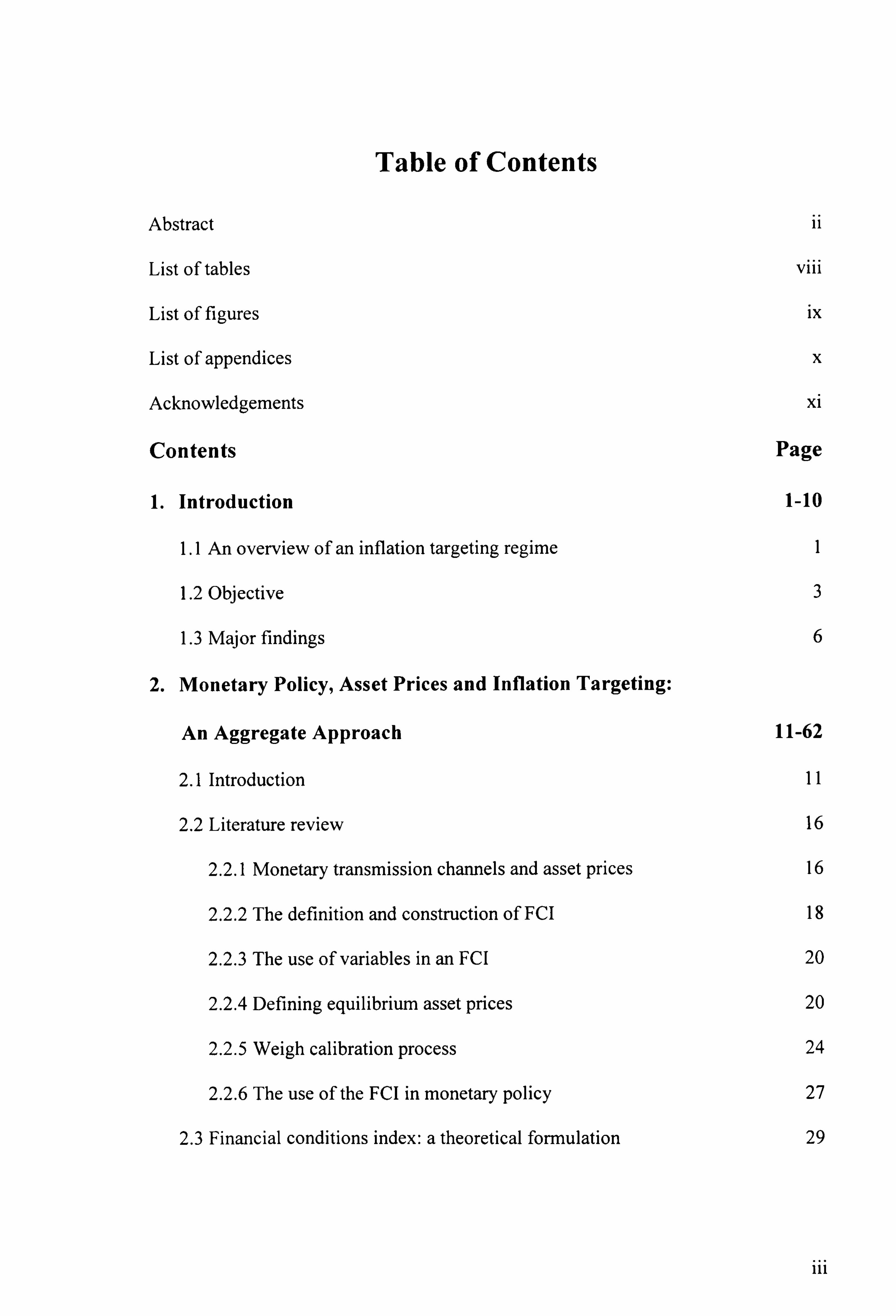
Abstract
Inflation targeting has been the central focus of monetary policy since early 1990s as
more than 60 central banks across the countries target it explicitly, others target it
implicitly. However, how precisely does the central bank target inflation in practice? Does monetary policy always only respond to inflation or does it also react to asset
prices and open economy variables? This thesis models these aspects of monetary
policy primarily focusing to the UK inflation targeting regime.
The empirical results are significant. First, monetary policy in UK is forward looking. It
responds to deviations of inflation from the target, to the output gap and to asset prices
misalignments. The policy reaction to inflation is strongest followed by the reaction to
the output gap, the foreign interest rate, the exchange rate, house prices and share
prices. Second, monetary policy is nonlinear because (a) it has deflationary bias, (b) it
responds to asset prices only when asset prices misalignments are high, and (c) it
responds to the output gap only when it does not respond to inflation and asset price
misalignments. Third, policy response to exchange rates does not depend on inflation
regime while the reaction to inflation does depend on the exchange rate regime. Fourth, policy response to inflation is asymmetric and it aims to keep inflation within a
range rather than pursuing a point target of 2.5%. Fifth, neither the exchange rate
misalignment nor the foreign interest rate alone can capture the open economy effects;
policy responds to both variables.
Page 3
Table of Contents
Abstract 11
List of tables viii
List of figures ix
List of appendices x
Acknowledgments xi
Contents Page
1. Introduction 1-10
1.1 An overview of an inflation targeting regime 1
1.2 Objective 3
1.3 Major findings 6
2. Monetary Policy, Asset Prices and Inflation Targeting:
An Aggregate Approach 11-62
2.1 Introduction 11
2.2 Literature review 16
2.2.1 Monetary transmission channels and asset prices 16
2.2.2 The definition and construction of FCI 18
2.2.3 The use of variables in an FCI 20
2.2.4 Defining equilibrium asset prices 20
2.2.5 Weigh calibration process 24
2.2.6 The use of the FCI in monetary policy 27
2.3 Financial conditions index: a theoretical formulation 29
111
Page 4
2.3.1 Structural model 30
2.3.2 Inflation targeting 32
2.3.2.1. Strict CPI inflation targeting framework 33
2.3.2.2. Domestic inflation targeting framework 36
2.4 Empirical estimates of the financial conditions index 40
2.4.1 Data generating process and unit root test 40
2.4.2 Estimation and interpretation 43
2.5 Monetary policy reaction function and the use of FCI 51
2.5.1 Basic Taylor rule 51
2.5.2 Augmented Taylor rule 53
2.5.3 Estimation procedure 55
2.5.4 Empirical findings 56
2.6 Concluding remarks 61
3. Modelling UK Monetary Policy: A Nonlinear Perspective 63-113
3.1 Introduction 63
3.2 Evolution of monetary policy reaction function 66
3.2.1 Linear reaction function 68
3.2.2 Nonlinear reaction functions 70
3.3 Methodology 74
3.3.1 General strategy and modelling framework 74
3.3.2 Benchmark specification 75
IV
Page 5
3.3.2.1. Taylor rule 75
3.3.2.2. Augmented Taylor rule 77
3.3.3 Nonlinear modelling 79
3.3.3.1. Size and sign asymmetries 79
3.3.3.2. Smooth transition autoregressive models 81
3.4 Empirical estimates and discussion 89
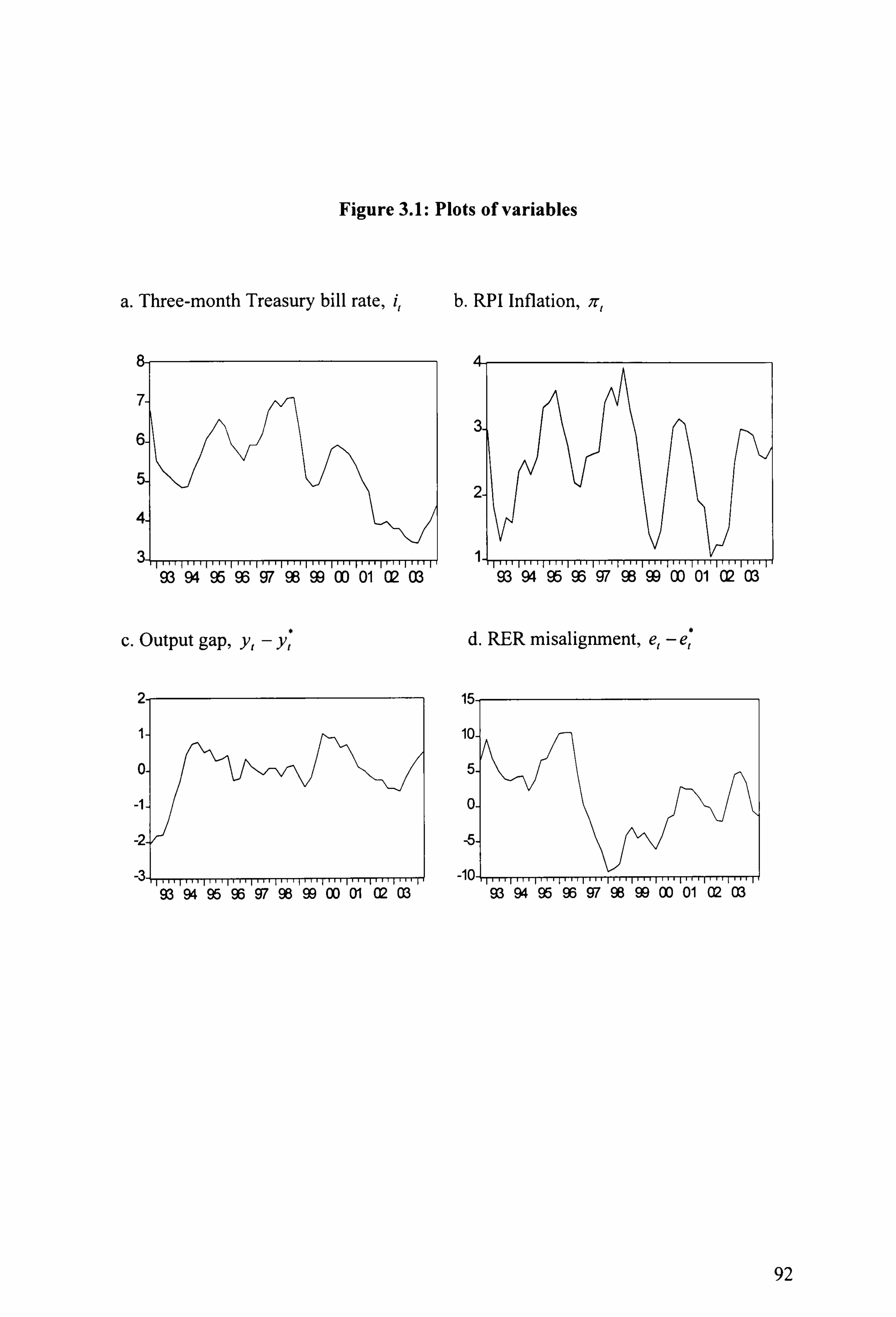
3.4.1 The data 89
3.4.2 Linear estimates 93
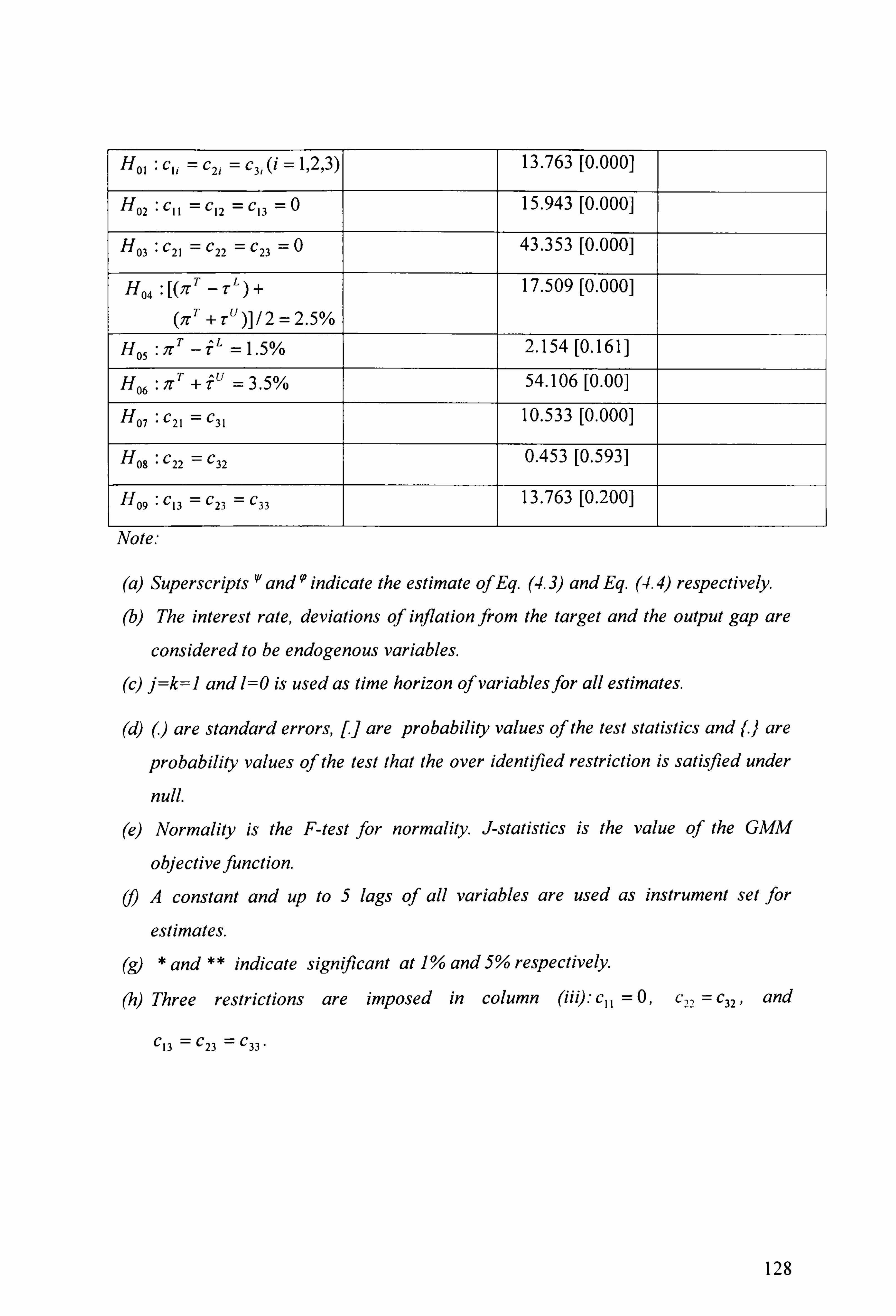
3.4.3 Nonlinear estimates 98
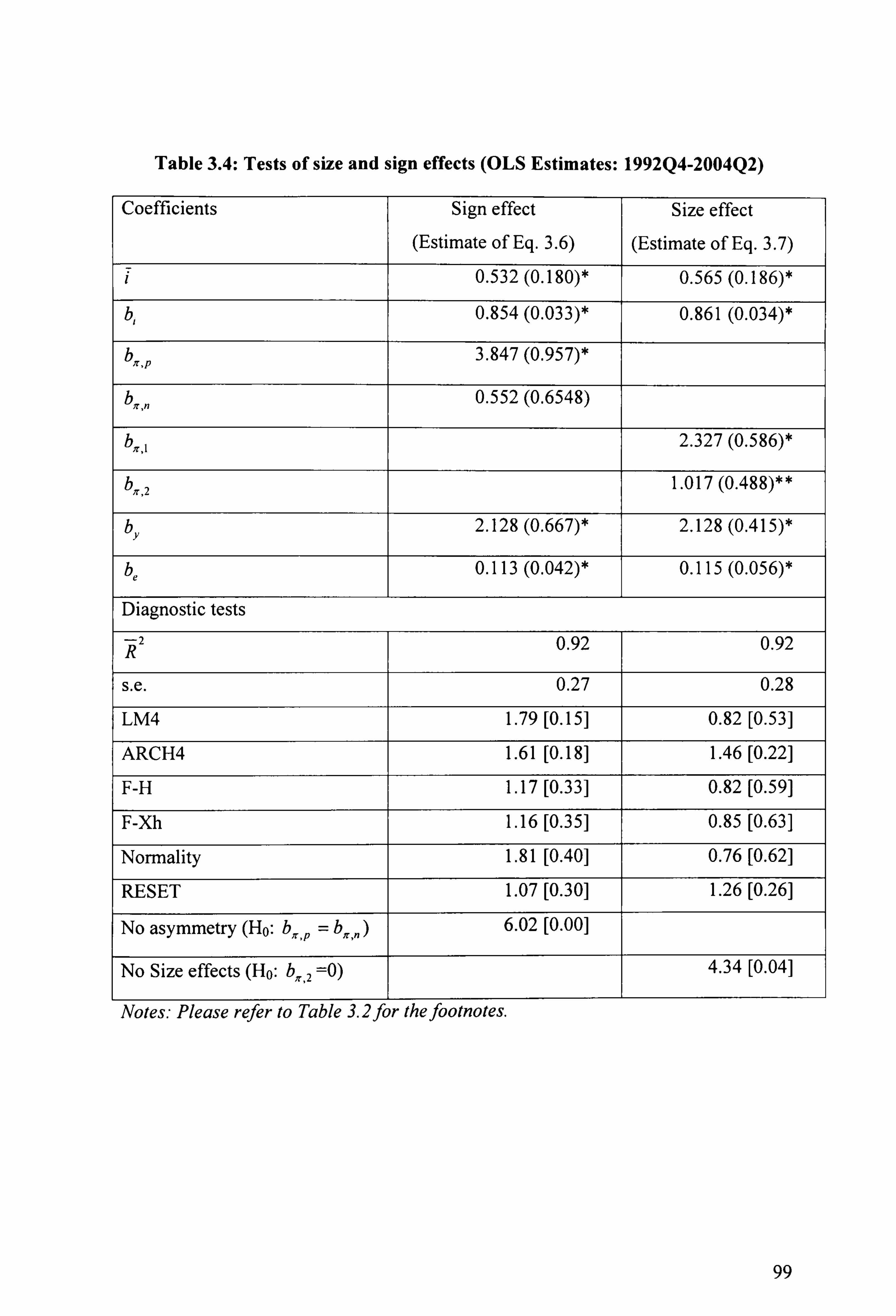
3.4.3.1 Accounting for sign and size asymmetries 98
3.4.3.2 Formal nonlinearity tests 100
3.4.3.3 Estimates of nonlinear reaction functions using STAR models 103
3.5 Conclusion III
4. Nonlinear and Asymmetric Monetary policy in UK:
Evidence from the open economy Taylor rule 114-139
4.1 Introduction 114
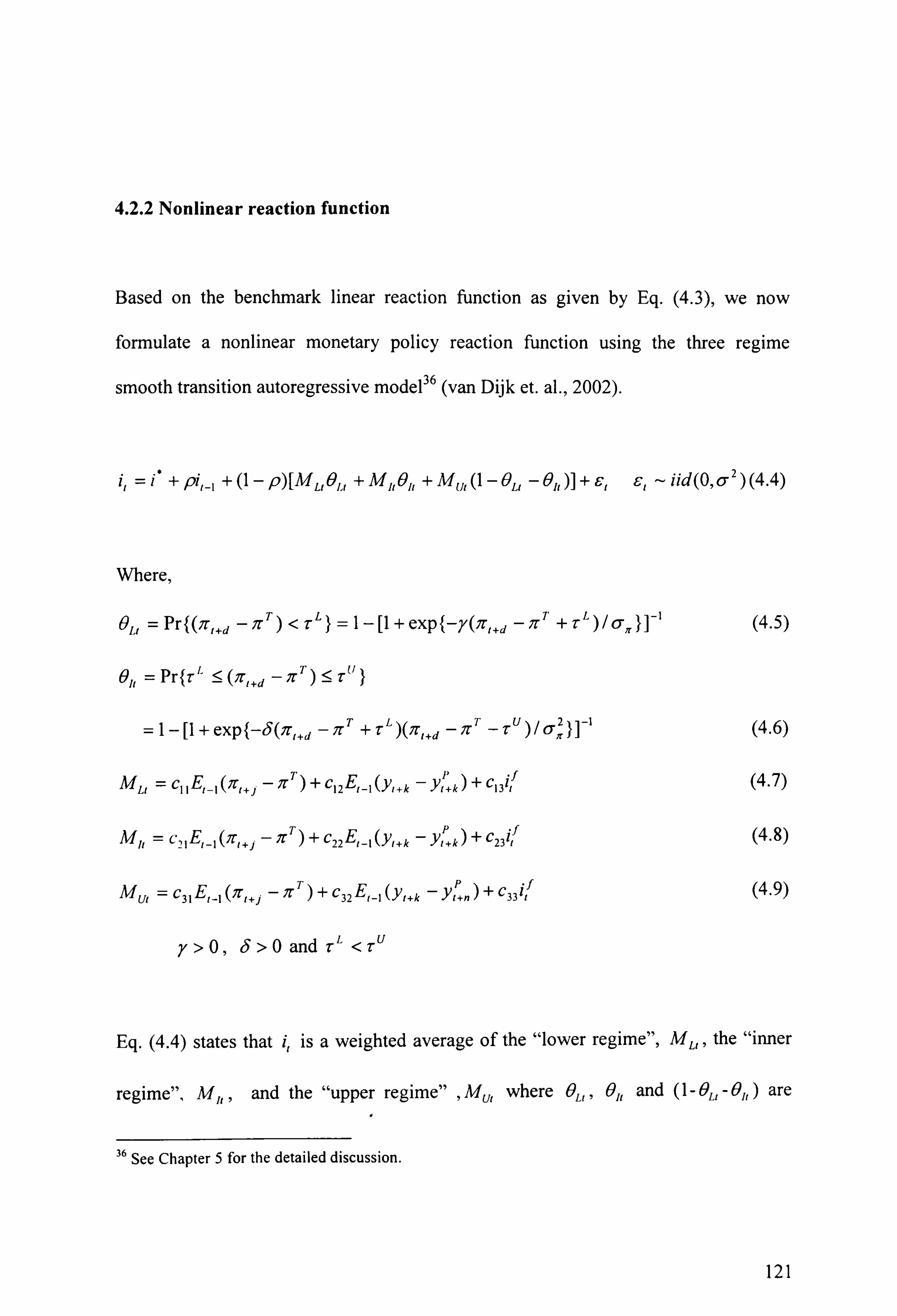
4.2 Methodology 118
4.2.1 Linear reaction function 118
4.2.2 Nonlinear reaction function 121
4.3 The data 124
4.4. Empirical results and discussion 126
4.5. Classification of observations 132
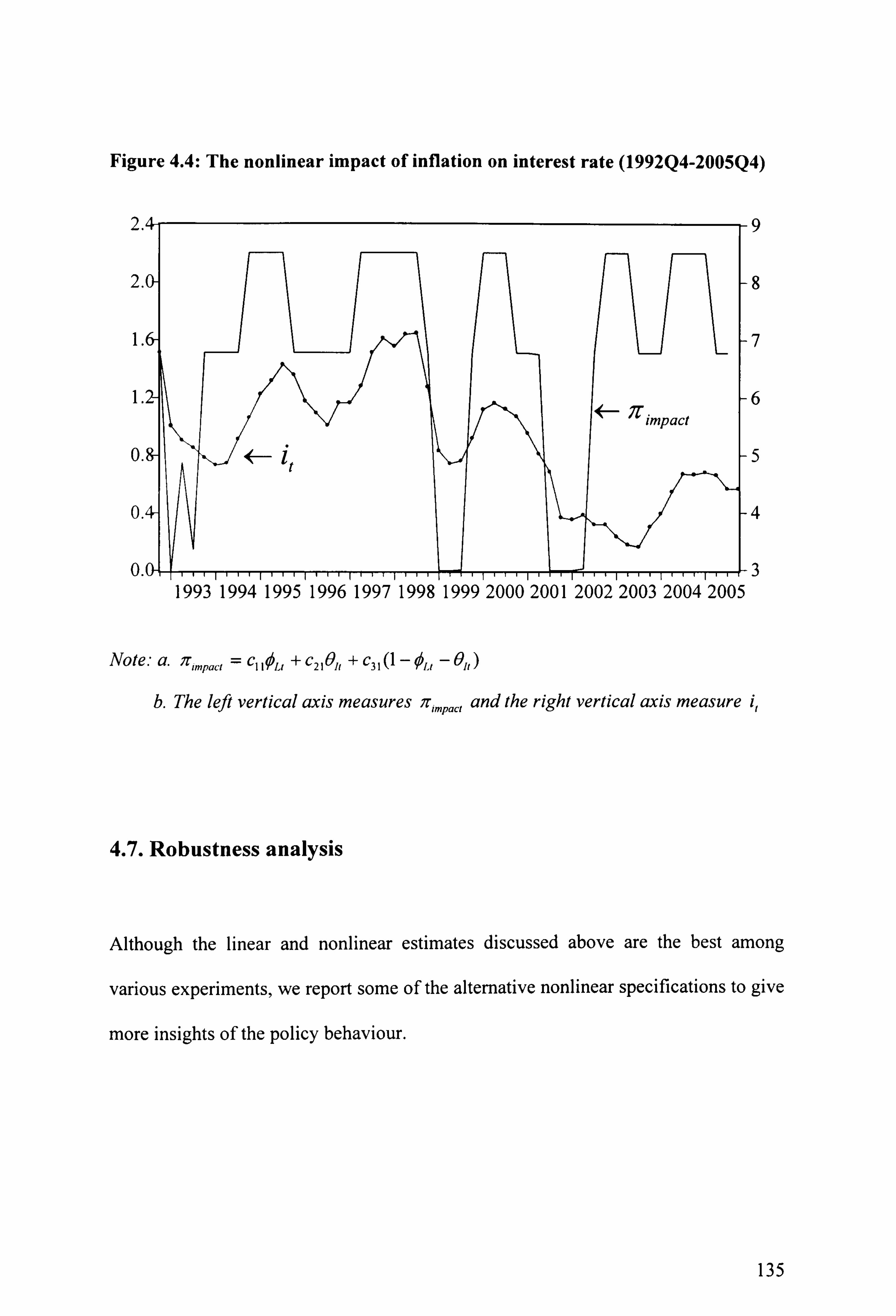
4.6. Impact analysis 134
V
Page 6
4.7. Robustness analysis 135
4.8. Conclusion 138
5. The complex response of Monetary Policy 140-178
5.1 Introduction 140
5.2 Multiple-regime STAR models in economics 143
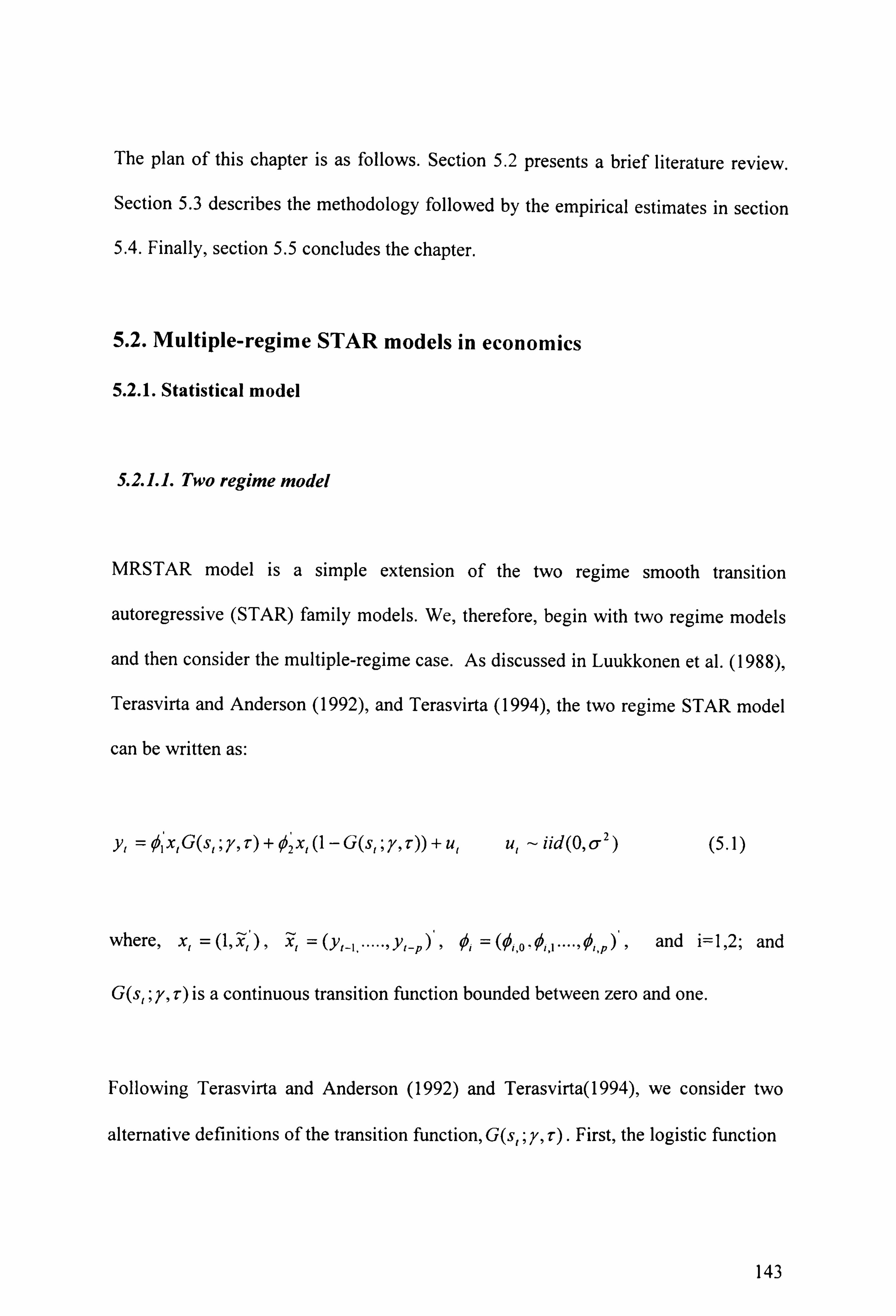
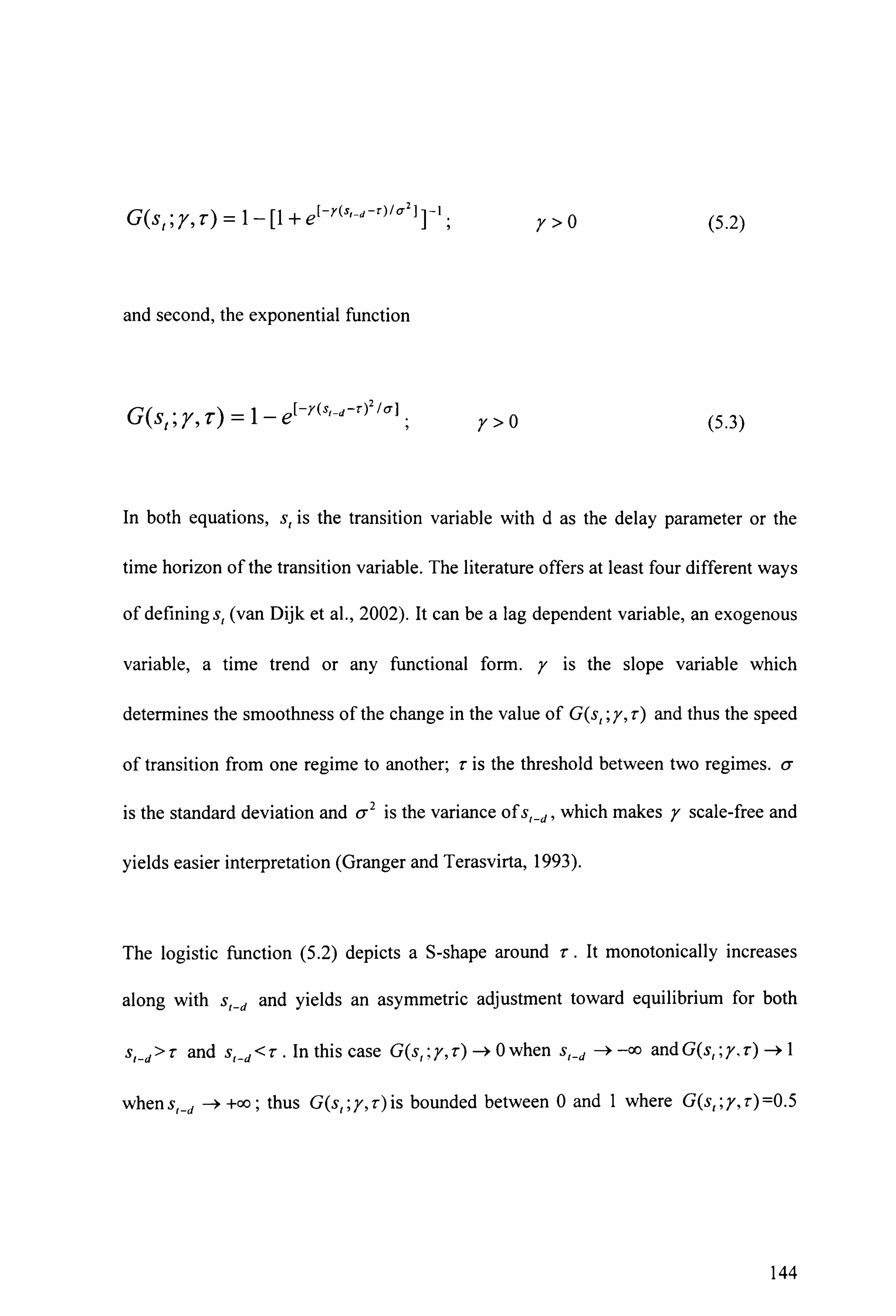
5.2.1. Statistical model 143
5.2.1.1. Two regime model 143
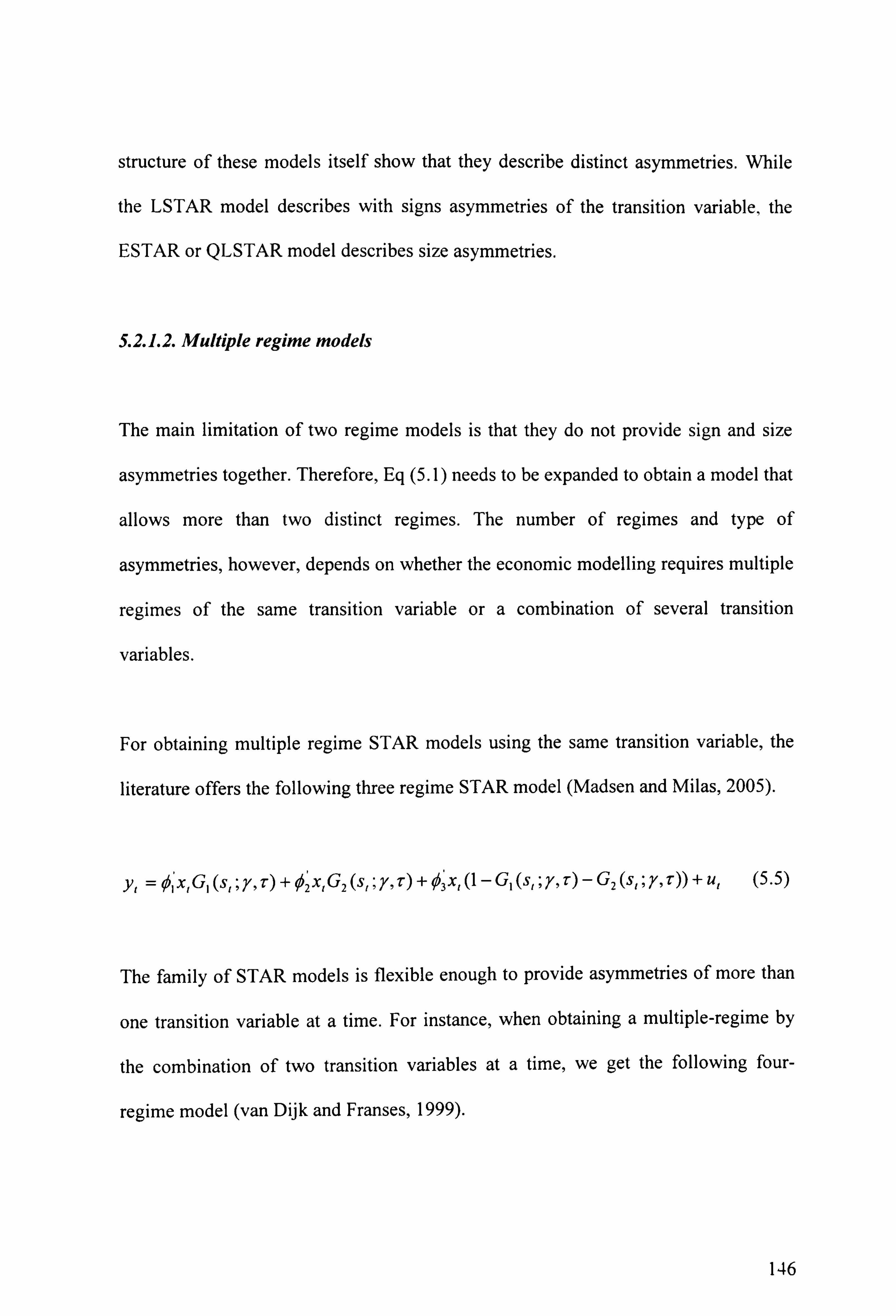
5.2.1.2. Multiple regime models 146
5.2.2. The importance of STAR models 148
5.2.3 The use of multiple regime STAR models in economics 149
5.3 Methodology 151
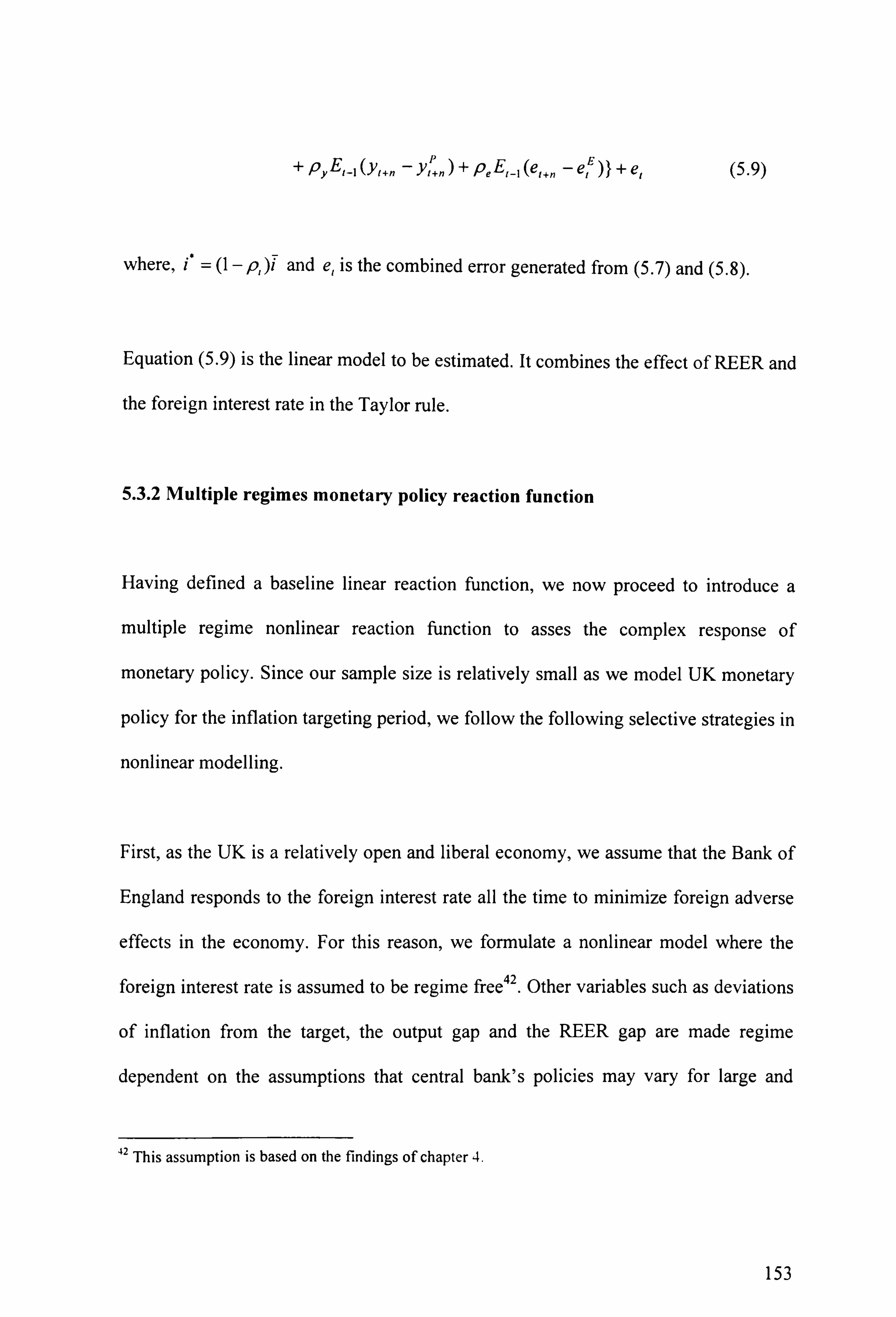
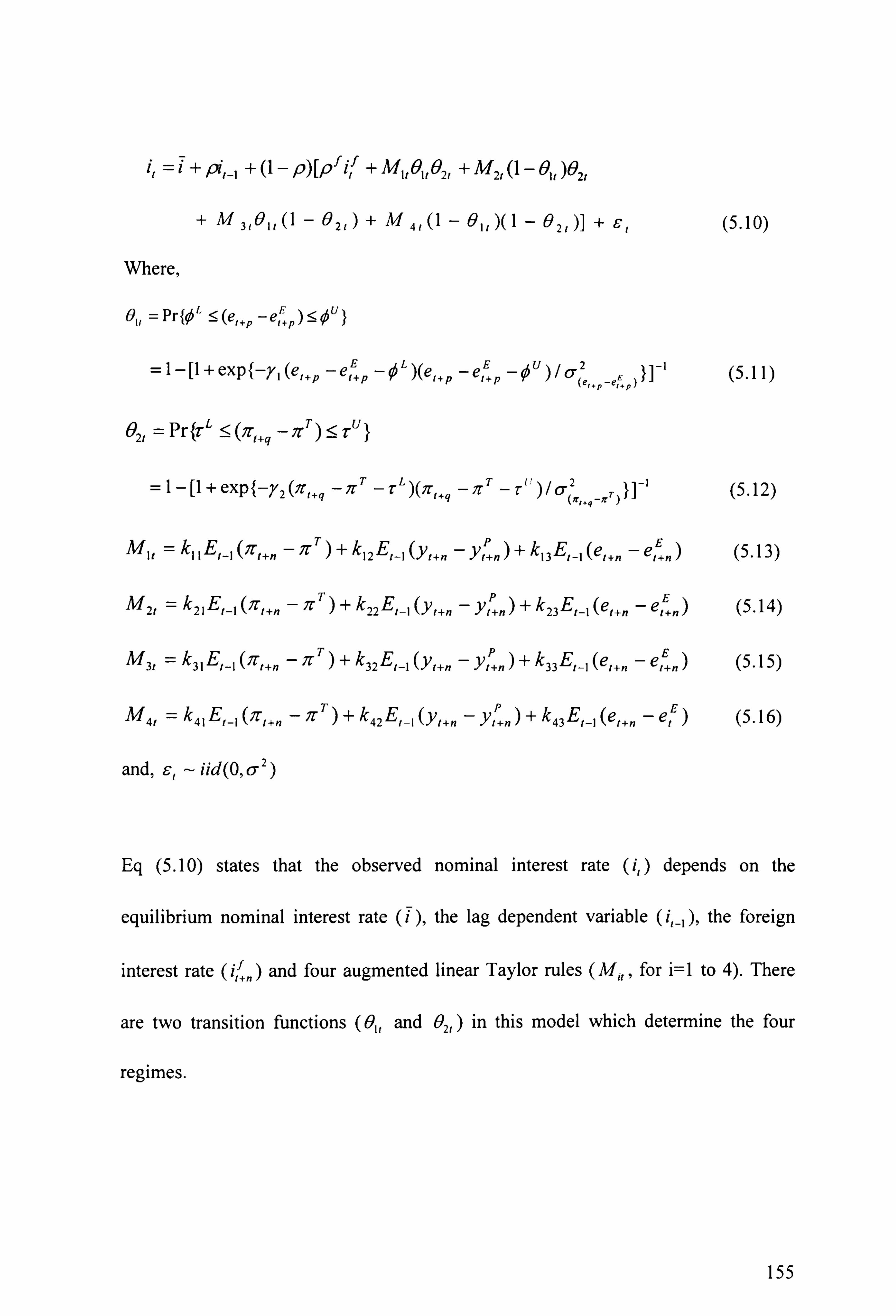
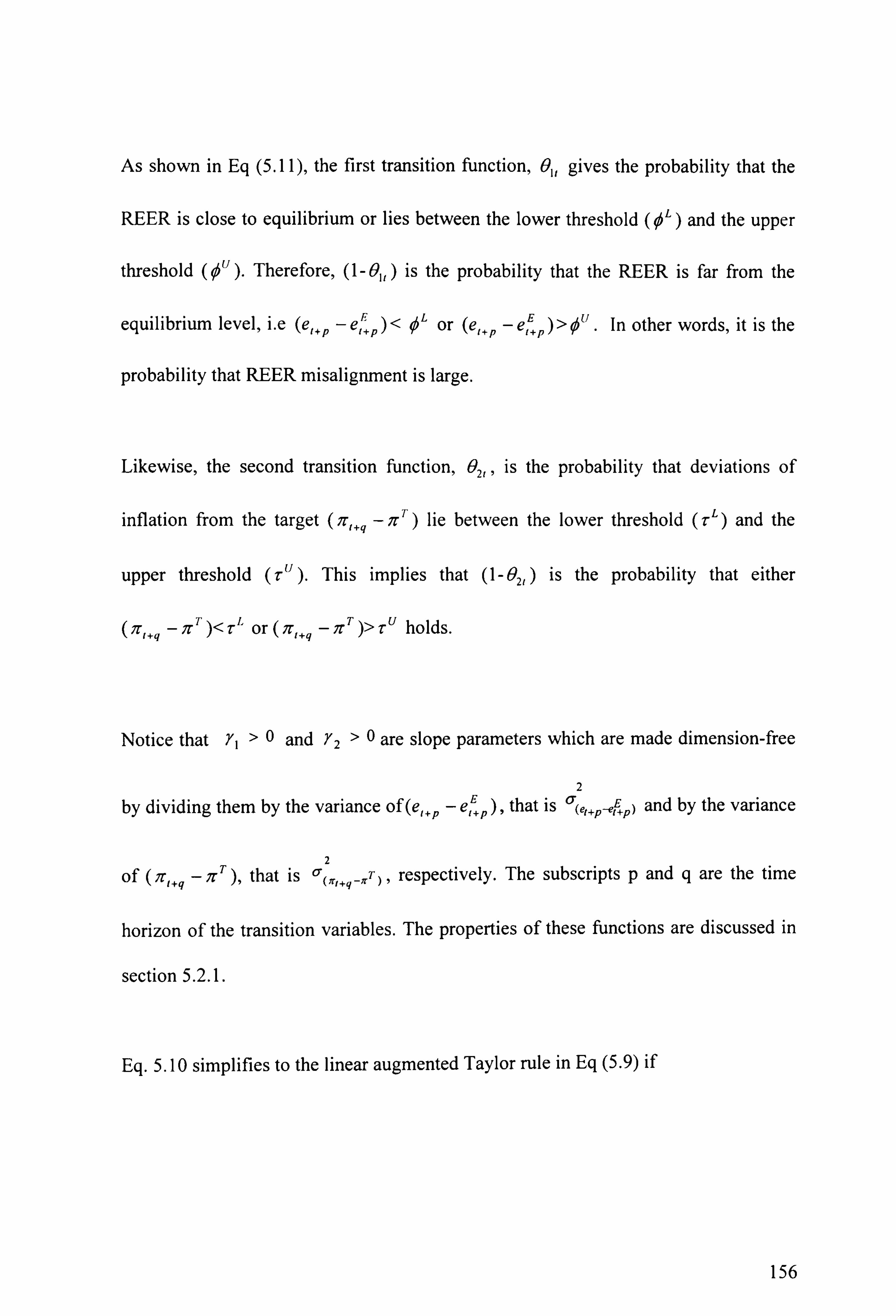
5.3.1 Linear monetary policy reaction function 151
5.3.2 Multiple regimes monetary policy reaction function 153
5.3.2.1. Interpretation of the model 157
5.3.2.2. Features of nonlinear policy rules 158
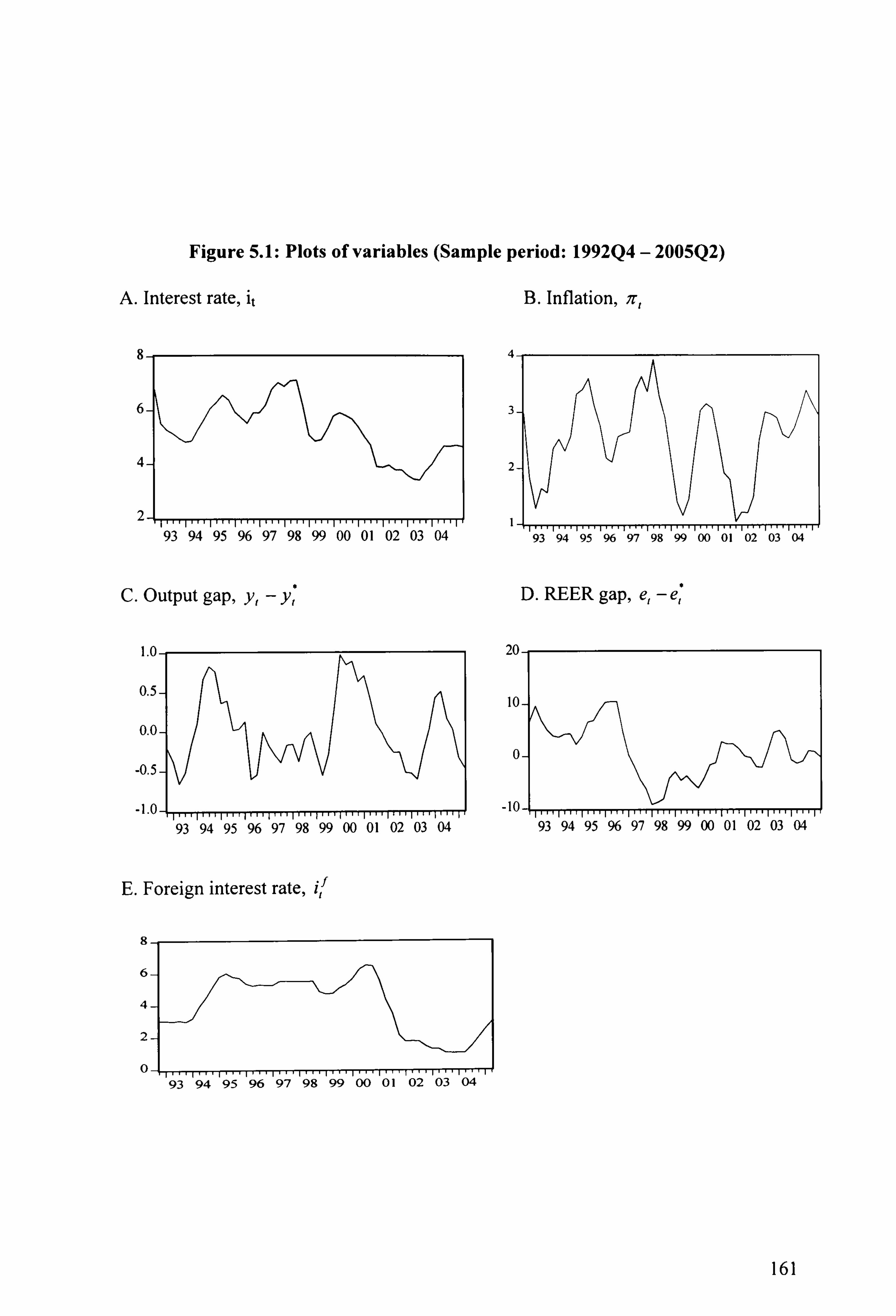
5.4 Empirical estimates 160
5.4.1 The data 160
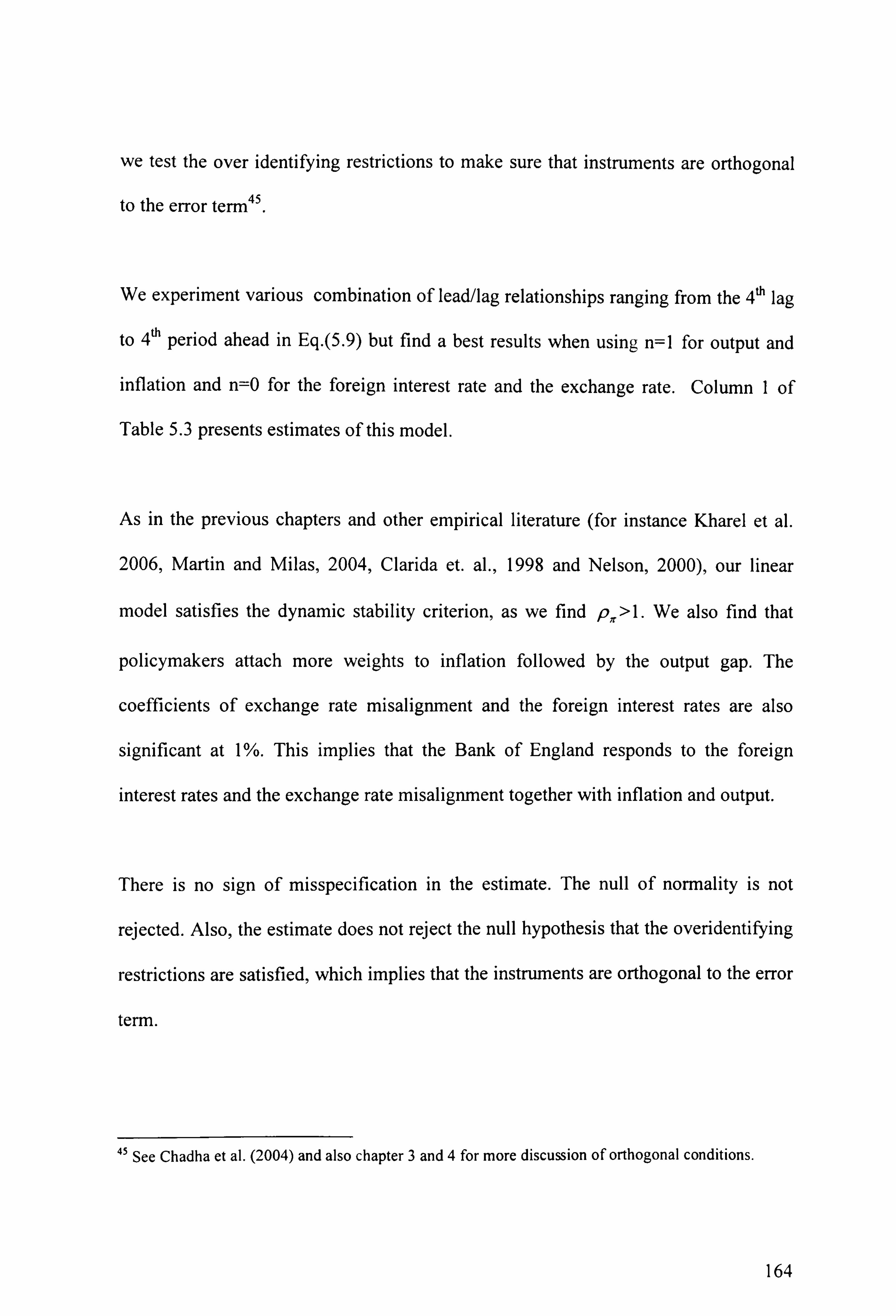
5.4.2 Linear estimates 163
5.4.3. Nonlinear estimates 166
5.4.3.1 General strategy 166
5.4.3.2 The estimates and discussion 167
5.4.3.3 Classification of observations by regime 172
5.4.4 Sensitivity analysis 175
vi
Page 7
5.5 Concluding remarks
6. Summary and Conclusion
Selected references
Appendices
176
179-185
186-203
204-215
Vil
Page 8
List of Tables
Table headings Page
Table 2.1: The composition of the FCI in the literature 22
Table 2.2: Comparison of FCl/MCls weights 39
Table 2.3: ADF test (I 979Q I to 2003Q4) 42
Table 2.4: Philips curve estimates 44
Table 2.5: IS curve estimates 46
Table 2.6: FCI weights 48
Table 2.7: UK Taylor rule: GMM estimates 57
Table 2.8: US Taylor rule: GMM estimates 59
Table 3.1: Unit root tests (I 992Q4 - 2004Q2) 91
Table 3.2: Estimates of linear reaction functions (1992Q4-2004Q2) 94
Table 3.3: The estimates of expanded Taylor rule (I 992Q4-2004Q2) 97
Table 3A Tests of size and sign effects (OLS Estimates: 1992Q4-2004Q2) 99
Table 3.5: Formal linearity test (I 992Q4-2004Q2) 103
Table 3.6: Estimates of nonlinear monetary policy reaction function 104
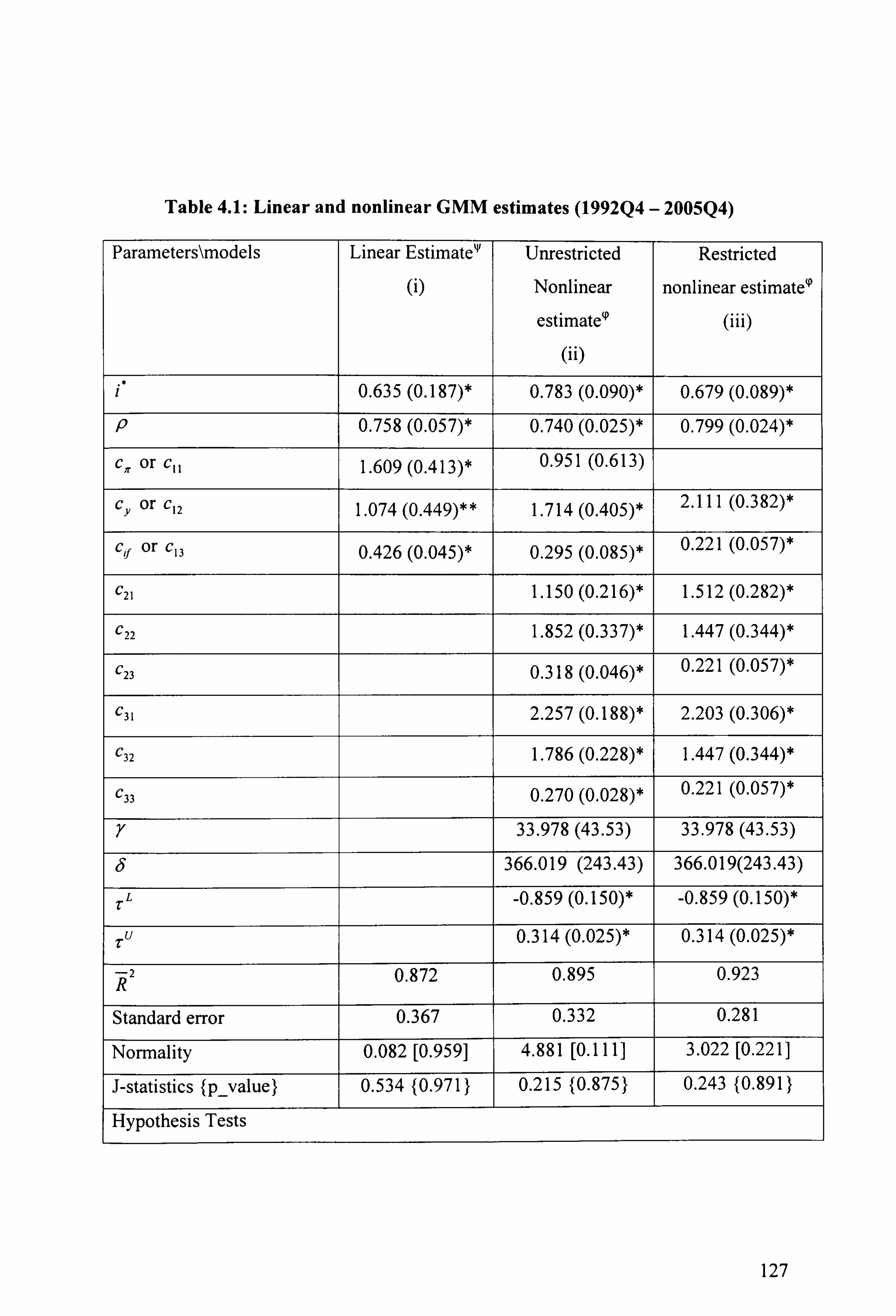
Table 4.1: Linear and nonlinear GMM estimates (I 992Q4 - 2005Q4) 127
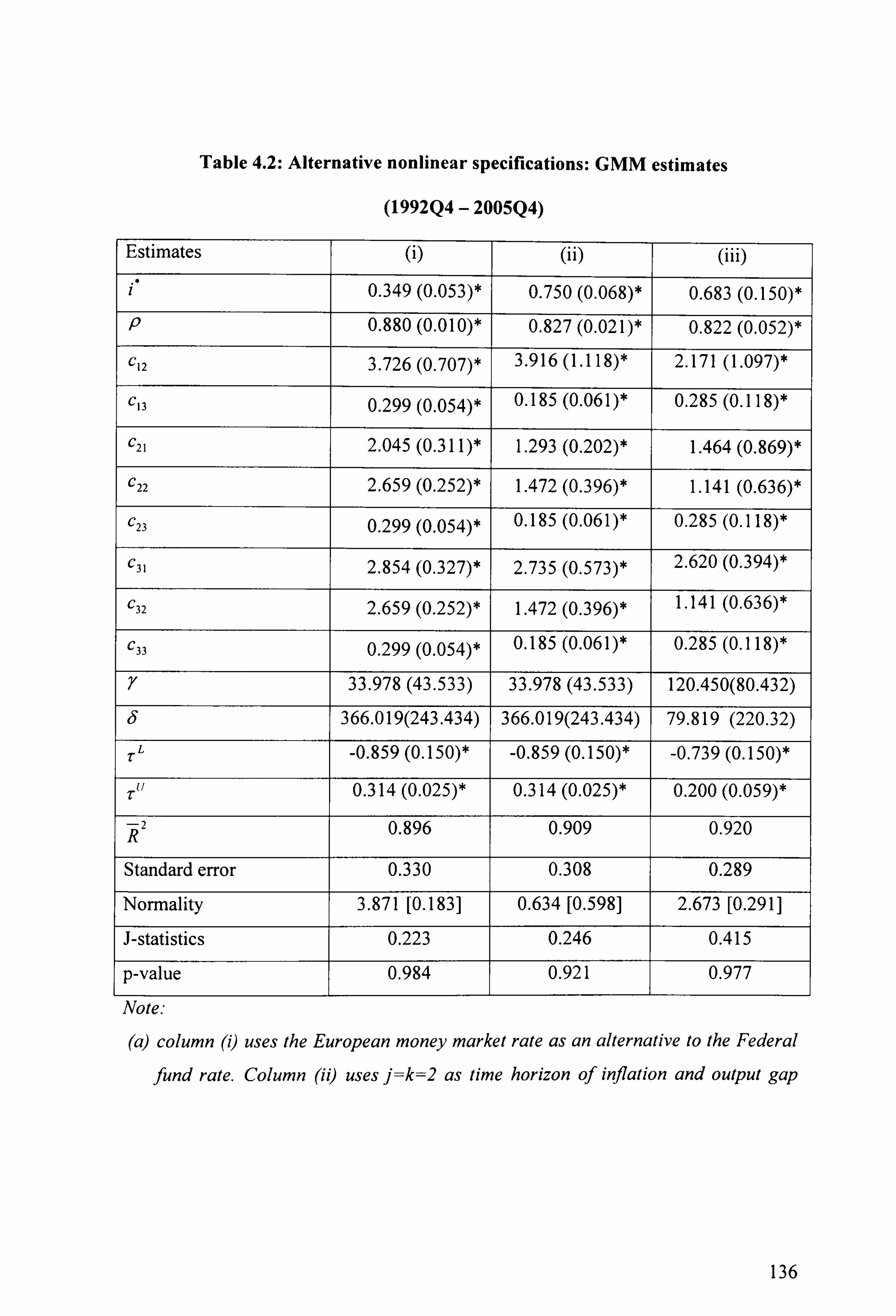
Table 4.2: Alternative nonlinear specifications: GMM estimates 136
Table 5.1: Synthesis of nonlinear monetary policy 159
Table 5.2: Unit root tests (Sample period: 1992Q4 - 2005Q2 163
Table 5.3: Linear reaction functions: GMM estimates (1992Q4-2005Q2) 165
Table 5.4: Nonlinear reaction functions: GMM estimates (I 992Q4-2005Q2) 169
viii
Page 9
List of Figures
Figure headings Page
Figure 2.1 UK: Financial Conditions Indices 50
Figure 2.2 USA: Financial Conditions Indices 50
Figure 3.1: Plots of variables 92
Figure 3.2: Plots of partial autocorrelation 101
Figure 3.3: Plots of inflation against thresholds 109
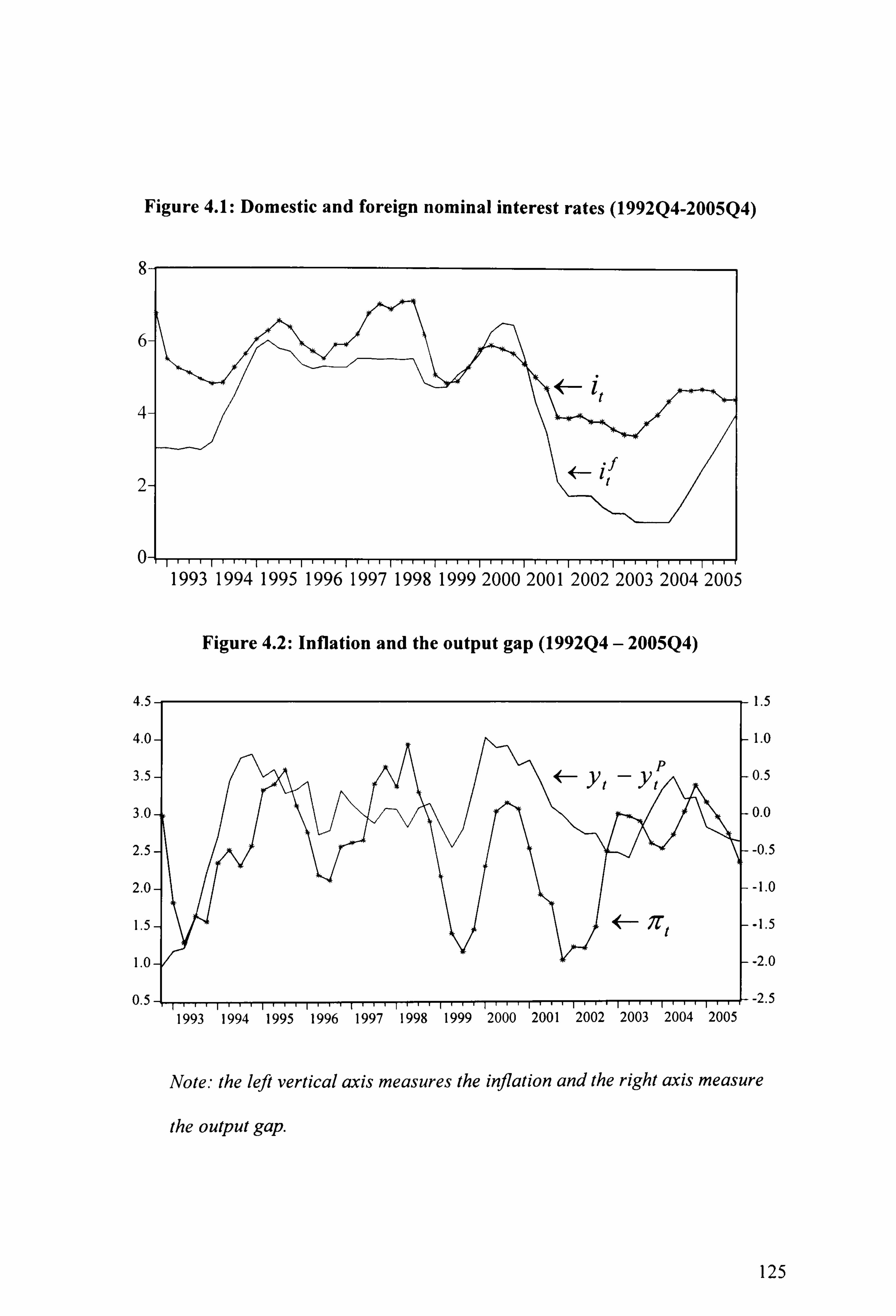
Figure 4.1: Domestic and foreign nominal interest rates (I 992Q4-2005Q4) 125
Figure 4.2: Inflation and the output gap (1992Q4 - 2005Q4) 125
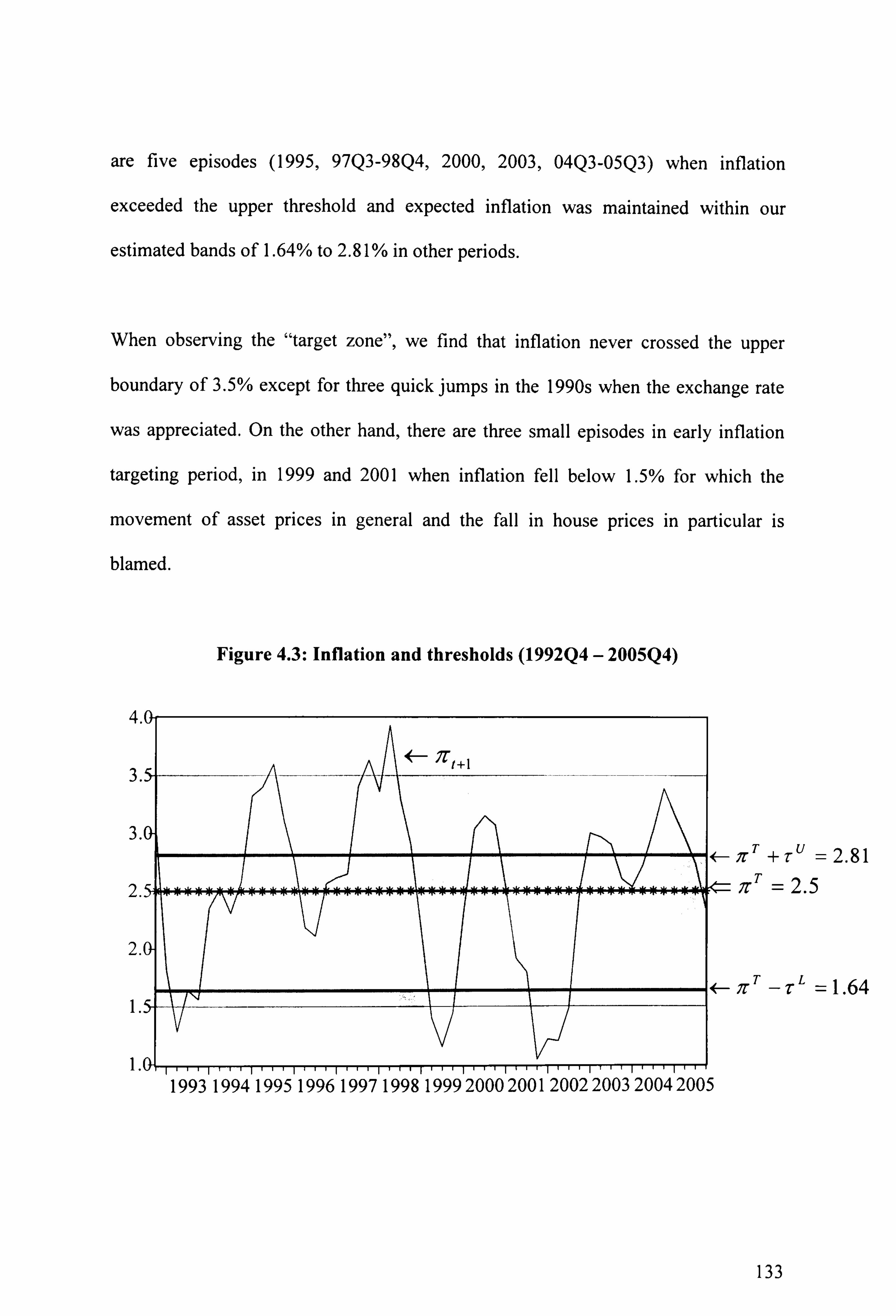
Figure 4.3: Inflation and thresholds (I 992Q4 - 2005Q4) 133
Figure 4.4: The nonlinear impact of inflation on interest rate (1992Q4-2005Q4) 135
Figure 5.1: Plots of variables (Sample period: 1992Q4 - 2005Q2) 161
Figure 5.2: Distribution of asset prices (transition variables) over regimes 173
Figure 5.3: Classification of interest rate in different regimes 174
ix
Page 10
List of Appendices
Appendix headings Page
Appendix 2.1: Definition and sources of variables 204
Appendix 2.2: Unit Root Tests 205
Appendix 2.3: MCI weights 209
Appendix 2.4: UK: Monetary Conditions Indices 210
Appendix 2.5: USA: Monetary Conditions Indices 211
Appendix 3.1: Alternative specifications of nonlinear reaction ftinctions 212
Appendix 3.2: Alternative estimate of nonlinear reaction functions 213
Appendix 5.1: Classification of monetary policy by Regimes 215
x
Page 11
Acknowledgments
I am extremely grateful to my principal supervisor, Professor Christopher Martin, for
his invaluable guidance without which this research would not have been completed
in this form. I am also grateful to my second supervisor Dr. John Hunter for his
guidance. Likewise, I am thankful to all faculty members and administrative staffs in
the Economics and Finance Department for their support.
There are numbers of individuals and institutions who extended their co-operation
towards me during this study period. I am indebted to Professor Kul Bahadur Luintel,
Cardiff University, the former PhD Convener at Economics and Finance Department,
Brunel University, for his intellectual as well as personal guidance. Similarly, I am
grateful to Professor Costas Milas, Keele University, for his stimulating comments on
Chapter 3 and 5.
I am thankful to the internal seminar participants at Brunel University (UK), summer
school participants at University of Bonn (Germany), conference participants at the
London School of Economics (UK) and workshop participants at University of Udine
(Italy) for their creative comments on my presentations based on this thesis. Financial
support from the Nepal Rastra Bank (central bank of Nepal) for the first year and a
bursary and teaching assistantship from the Brunel University for the remaining years
are greatly acknowledged.
xi
Page 12
Thanks go to my PhD colleagues Rekha Kharel, Rupak Shrestha, Muslimin Anwar
and Julian William (Bath University) for their helpful suggestions and everlasting
discussion on my research. I am also thankftil to Dr. Subhash Pokhrel, Binaya
Bastola, Devendra Upadhyaya, Kumar Sapkota and Deepak Khatiwada for their co-
operation.
Finally, I would like to take this opportunity to express my heartfelt thanks to Dr.
Yuba Raj Khatiwada (father-in-law) and family for their moral, financial and family
support, which, I believe, have played a pivotal role to complete this study. I can't
express all my feelings and gratitude to them in words. Similarly, my sincere
gratitude goes to my parents (Deva Raj and Sundar laxmi), sister Asmita and daughter
Riya who are my inner source of inspirations and who endured the pain of my
absence from home. Last, but not least, very special thanks, from the bottom of my
heart, goes to my wife Rita for her fascinating love and care that brought my
endeavour towards success.
Thank you.
xii
Page 13
Chapter 1
Introduction
1.1 An overview of an inflation targeting regime
Although a number of central banks have targeted inflation since the early 1990s, the
idea was suggested for more than a century ago. As discussed in Haldane (1995),
Alfred Marshall suggested a monetary system that adjusted to fix the purchasing
power of each unit of currency closely to an absolute standard as early as in 1887
(Marshall, 1887). Wicksell (1898) advocated an explicit price-level standard for
monetary policy that was, later on, implemented by Sweden for about three decades in
the beginning of the I 9th century (see also Fisher, 1922).
Historically, monetary policy had various objectives across countries until Bretton
Woods agreement to the exchange rate stability in July 1944. Under this agreement,
member countries were required to maintain the exchange rate of their currency
Page 14
within a fixed value - plus minus one percent - in terms of gold'. Following the
United States' suspension of convertibility from dollars to gold due to its budget and
trade deficits, the Bretton Woods agreement collapsed in 1972.
The objective of monetary policy then gradually refocused to economic stability in
general and financial stability including price stability in particular through targeting
monetary aggregates (Friedman, 1977). Although some central banks still target
monetary aggregates, it did not remain in place for a long time in many countries
(IFS, 2005).
Following the failure to stabilize inflation through the exchange rate and monetary
aggregates, a growing number of central banks adopted inflation targeting in the early
1990s. There is now a consensus among policyrnakers, economists, and general public
that low and predictable inflation helps to promote economic efficiency and growth in
the long run. It is also argued that macroeconomic stability in general and price level
stability in particular are important preconditions for economic growth (Fisher, 1993).
It is also accepted that monetary policy can affect only inflation, and not the real
variables such as output or unemployment in the long run (Bernanke et. al., 1999).
According to this school of thought, one of the reasons for a high level of inflation
1 This is an agreement on the exchange rate stability made in the United Nations Monetary and
Financial conference at Bretton Woods, Washington, in July 1994 by 730 delegates from 44 countries.
The agreement, later on, was ratified by other member countries of the UN (Bank of Canada, 200 1).
2
Page 15
during 1970s and 1980s was the outcome of the attempt to manipulate Philips curve
(Philips, 1958). Moreover, Friedman (1977) argues that there is no long run trade-off
between inflation and unemployment as expansionary monetary policy results only
inflation. The recent speeches of the central bankers and economists suggest that
central banks have no choice other than targeting inflation either implicitly or
explicitly to keep economy healthier.
Nowadays, more than 60 central banks, both from developed and emerging
economies, target inflation explicitly while other targets it implicitly 2 (Mahadeva and
Sterne, 2002). This framework of monetary policy aims to achieve an ex-post inflation
rate. However, as pointed out by Masson et al., (1997), the success of inflation
targeting depends on transparency, the ability of the central bank to carry out an
independent monetary policy and the absence of a commitment to have another
nominal anchors like the exchange rate or to economic growth (see also Bernanke et
al., 1999).
1.2 Objective
Although the rate of inflation has remained relatively low and stable in the inflation
targeting regime, economic stability is largely influenced by foreign economic shocks
and asset price volatility. The contagion effects of the financial and banking crisis
during some periods in 1990s, a frequent oil price shocks from the middle-east
See also ITS 2005 Year Book, IMF.
3
Page 16
countries, and the development of world financial markets threatened stability. On the
domestic front, stock prices and house prices in major industrial countries rose to
record levels during this period. These have generated the following lively debates in
the literature whether or not monetary policy should and/or does respond to open
economy effects and asset prices.
First, the recent literature argues that monetary policy may be nonlinear. This implies
that policy does not respond to inflation constantly and uniformly all the time; it may
respond to other variables when it does not have to respond to inflation (see chapter 3
for more discussion). For example, Martin and Milas (2004) argue that monetary
policy does not respond to inflation when the expected inflation is close to the target.
Dolado at el. (2002) argue that policy reaction to the output gap differs between
positive and negative output gaps. This class of literature, however, does not describe
as how monetary policy behaves when inflation is close to the target or when policy
does not have to respond to inflation. Does policy respond to some other variables or
remain idle? At the same time, we suspect whether nonlinearity is observed in the
literature due to misspecification in the usual Taylor rule.
Second, the literature debates whether monetary policy responds to asset prices.
Some argue that asset prices are an integral part of monetary policy and that policy
should respond to them in a similar way it responds to inflation and the output gap
while others believe that asset prices should be taken into account only to the extent
that they help forecasting inflation (see Chapter 2 for references and more discussion).
4
Page 17
In either case, the literature, to our knowledge, does not analyze whether policy differ
between the periods of a large appreciation and depreciation of asset prices.
Third, there is also a debate on as how monetary policy responds to the open
economy. Some papers argue that policy responds to the short-term foreign interest
rate while others argue that it responds to the real exchange rate or the real exchange
rate misalignment as an alternative to the foreign interest rate (see Chapter 3 and 4 for
the references and more discussion).
In this context, we investigate some of these issues discussed above. In particular, the
main aim of this research is
(a) to investigate whether monetary policy responds to asset prices. If so, to what
extent and whether the policy response depends on the state of inflation?
(b) to assess whether monetary policy targets inflation precisely in a way it is
announced. In the process we analyze whether policy is forward or backward
looking, linear or nonlinear, point target vs. range target, symmetric vs.
asymmetric; and
(c) to analyze whether monetary policy responds to foreign interest rates and real
exchange rate misalignments; and whether the policy reaction to them depends
on the state of inflation.
5
Page 18
1.3 Major findings
The analysis begins with an investigation of whether or not monetary policy responds
to asset prices. We consider two approaches in this regard. We first assess whether
policy responds to asset prices collectively by responding to the financial condition
index (FCI) in chapter 2 and we then verify the findings of chapter 2 by estimating an
asset prices augmented Taylor rule in chapter 3.
In chapter 2, we construct FCIs, which are a weighted average of the interest rate, the
exchange rate, share prices and house prices. Instead of using a demand curve for
obtaining FCls as in the conventional literature, we propose that an open economic
structural model be used. We provide two alternative weighting procedures, one for a
strict CPI inflation targeting framework and another for a flexible inflation targeting
framework.
We construct FCls for the US and the UK using quarterly data over 1979QI to
2003Q4 and then estimate a FCI augmented Taylor rule. Our empirical results show
that FCIs are very useful for describing the monetary policy stance in these two
countries.
We then estimate asset price augmented reaction functions in Chapter 3 as an
alternative to the FCl augmented Taylor rule in Chapter 2. The asset prices we
consider in this chapter are similar to those of chapter 2 as we use exchange rate
6
Page 19
misalignment, deviations of house prices from trend and deviations of share prices
from the fundamental. Our results overwhelmingly suggest that the asset price
augmented Taylor rule outperforms a simple rule. Overall, we obtain a consistent
conclusion from both chapters (chapter 2 and 3); monetary policy responds to asset
prices.
Chapter 3 also aims to investigate whether or not monetary policy is nonlinear and
whether or not it responds to exchange rate misalignments. It employs various
nonlinear models including the smooth transition autoregressive (STAR) model to
asses nonlinearity in monetary policy. Chapter 4 ftirther models UK monetary policy
using three regimes STAR model. This chapter mainly seeks to analyze whether
monetary policy responds to foreign monetary policy by responding to the foreign
short-term interest rates. As we find that the BoE responds to the exchange rate
misalignment in chapter 3 and to the foreign interest rates in chapter 4, we then
include both variables in the reaction function in chapter 5 and employ a four regime
STAR model. The empirical findings can be summarized as follows:
First, we find that monetary policy is forward looking. The empirical estimates
throughout this research constantly suggest that one quarter ahead forward looking
Taylor rule outperfonns any other specification.
Second, the policy reaction to inflation is strongest followed by the response to the
output gap, the foreign interest rate, the exchange rate, house prices and share prices.
7
Page 20
Third, we find that policyrnakers aim to keep inflation within a range rather than
pursing a point target in practice.
Fourth, monetary policy does not respond to inflation when the expected inflation is
less than the lower threshold. On the other hand, the policy response to inflation is
vigorous when expected inflation exceeds the upper threshold. These imply that
monetary policy is deflationary bias. Moreover, we find that the upper inflation
threshold is just slightly higher than the target of 2.5% but the lower threshold is far
below the target though the BoE has to give a formal clarification to the government
if inflation deviates for more than 1% in either direction from the target, suggests
monetary policy is nonlinear and policy response is asymmetric.
Fifth, monetary policy in the UK considers a separate exchange rate regime together
with inflation regime. The BoE responds to inflation and exchange rate only when
they are in their outer regime. More precisely, the Bank responds to the exchange rate
only if domestic currency under-valuation is greater than 4% or over-valuation
exceeds 5%. Similarly, policy responds to inflation only when expected inflation is
less than 1.9% or greater than 2.8%.
Sixth, the monetary policy response to exchange rate misalignments does not depend
on inflation regime but the response to inflation does depend on the exchange rate
regime.
8
Page 21
Seventh, policyrnakers respond to the output gap only when they do not respond to
asset prices or inflation, that is, when inflation and the exchange rates are in their
inner regimes.
Finally, we find that neither the exchange rate misalignment nor the foreign interest
rate alone can capture the open economy effects; monetary policy responds to both
variables. Unlike the policy response to exchange rate misalignments, we find that
policy reaction to the foreign interest rate is unaffected by the inflation or the
exchange rate regimes.
Although we use a standard analytical framework of monetary policy, our findings
should be taken cautiously while generalizing them for the following reasons:
First, it is argued that the perfon-nance of inflation targeting depends on the
institutional framework, operational procedure and the development of money and
financial markets, (see Bernanke et al., 1999). Therefore, our findings may not be
generalized to other central banks if the policy environment is different from that of
the BoE.
Second, the literature explores various policy rules to be employed to assess monetary
policy. Following the monetary policy committee (MPQ minutes of the BoE, we rely
on the interest rate reaction functions and do not attempt to compare them to any other
9
Page 22
alternative policy rules 3 (Taylor, 1993,1999 and Clarida et al, 1998). Our analytical
framework, therefore, can not be generalized to other countries if the interest rate rule
is not applicable to them.
Third, we do not make any argument as to whether or not monetary policy should
respond to asset prices and the international market as the literature debates this issue.
Our main focus is to analyze whether or not policy has been responding to them in
practice.
Fourth, there are numbers of crucial issues on the topic such as range target vs. point
target; price level vs. price changes target; impact of institutional autonomy to the
performance of inflation targeting; the definition of inflation to be considered; and the
criterion for setting the target range/value. We, however, do not attempt to address
any of them. We begin our analysis on the assumption that the central bank is free to
set monetary instruments to achieve the quantitative target which is already well
defined.
3 For example, some studies strongly advocate nominal income growth rule and monetary targeting
rules as an alternative to the interest rate rule (Taylor, 1999).
10
Page 23
Chapter 2
Monetary Policy, Asset Prices and Inflation Targeting:
An Aggregate Approach
2.1 Introduction
If the interest rate is the only effective monetary policy instrument in an open and
liberal economy and if inflation target is the only objective of monetary policy then
why be the central bank not just follow the Taylor rule (Taylor, 1993,1999) to respond
inflation? In practice, a number of monetary transmission channels work together
which may have a direct or indirect impact on inflation with differing magnitudes.
This implies that a proportional relationship between the interest rate and inflation
may not hold due to an involvement of other variables, possibly asset prices. For
instance, if overall economy is growing at above trend pace in a period of low
inflation, there would be a policy mistake if the interest rate is lowered in response to
II
Page 24
inflation (see also Dudley and Hatzius, 2000; Goodhart and Hofmann, 2001,2003
among others).
A large bulk of literature, therefore, argues that the simple Taylor rule is suboptimal in
an open economy because it does not consider the exchange rate and other asset prices
in the policy framework (see Ball 1999 and references therein). In fact, monetary
policy might take account of open economy effects and domestic financial markets by
responding to exchange rates, property prices and equity prices respectively at least for
three reasons. First, asset price misalignment may jeopardize financial stability, which
in turn may distort output and inflation (Goodhart, 2001 and Lowe, 2002). Second,
asset prices play an important role in the transmission of monetary policy. For instance
a rising asset price may have a direct impact on aggregate demand because asset prices
are associated with growing inflationary pressure (Montagnoli and Napolitano, 2005).
Third, asset prices contain important information regarding the future path of inflation
and output (Goodhart and Hofmann, 2003, Kontonikas and loannidis, 2005).
As discussed, there is a consensus in the literature that asset prices play an important
role in the economy. What is debatable is how and to what extent should monetary
policy respond to asset prices? There are three different views regarding this. The first
view is that asset prices should be made an integral part of monetary policy. Policy
should respond to them in a way it responds to inflation and the output gap (Cecchetti
et al., 2000). The second view is that asset prices should be considered only to the
extent that they help in forecasting inflation. As asset prices, in general, are more
12
Page 25
volatile than output and inflation, monetary policy may not be able to control inflation
if it responds to asset prices (Bernanke and Gertler, 1999). Finally, there is an
argument that policy should target a broader price index that includes asset prices
(Goodhart, 1999; Goodhart and Hofmann, 2003). Targeting a broader price index in a
way of targeting CPI inflation implies that policy responds to both inflation and asset
prices (Duguay, 1994).
To construct this broader price index, Freedman (1994), Duguay (1994) and Ball
(1999) propose a weighted average of the short-term interest rate and the exchange
rate that we know as the monetary conditions index (MCI). Under this approach,
policyrnaker attempts to set interest rates in order to keep the MCI in a par level or
within a range so as to maintain inflation and outpue. However, this index still
potentially neglects other transmission channels of monetary policy except for interest
rates and exchange rates.
In order to include domestic asset prices in the policy framework, Goodhart and
Hofmann (2001) develop a financial conditions index (FCI). This is a weighted
average of the short-term real interest rate, the real exchange rate, real house prices
and real share prices. This index is an extension of the MCI that includes house prices
and share prices in addition to MCI variables. Keeping the FCI in a specified range or
Since MCI keeps a strong positive relationship with inflation (Freedman, 1994).
13
Page 26
at a par level, therefore, implies that the central bank is also responding asset prices in
order to stabilize the inflation and output (Gauthier et. al., 2004).
In the light of this discussion, this chapter aims to give a different look regarding the
aggregate approach of monetary policy by introducing alternative measurements for
FCL Our motivations are the following.
First, the existing literature uses only the IS curve to obtain weights of asset prices
(eg. Goodhart and Hofmann, 2003, Lack, 2003) and excludes the supply side of the
economy. We argue that the FCl should be obtained from a macroeconomic structural
model, which combines both the supply and demand factors in the determination of
inflation and output.
Second, the conventional literature does not take into account of the direct impact of
changes in the real exchange rate while determining the FCI weights. We argue that
import prices may play a role in the determination of inflation in an open economy.
Third, the literature does not analyze whether the FCl framework is designed to target
the CPI inflation or other measure of inflation. We argue that the construction of FCI
weights should reflect the type of inflation that is targeted by the central bank.
This chapter addresses these issues on both theoretical and empirical grounds. We
develop two alternative FCI models, one for CPI inflation and another for domestic
14
Page 27
inflation targeting frameworks respectively. Although both of them are obtained from
a macroeconomic structural model, the main difference between them is the treatment
of the real exchange rate. The CPI model assumes that the real exchange rate has a
direct impact on inflation via import prices and indirect effects via pressure on the
aggregate demand while the latter case considers the indirect impact alone.
Second, we construct FCls for the UK and the USA using our new methodology and
compare them with the conventional method. The usefulness of indices is, then, tested
by estimating the FCI augmented Taylor rule. The empirical results overwhelmingly
suggest that the FCI contains important information for the monetary policy setting.
Finally, we find that the FCl augmented Taylor rules outperform the simple rule in
both countries irrespective to the type of FCls, implies that monetary policy responds
to asset prices.
The rest of the chapter is organized as follows. Section 2.2 reviews the existing
literature. Section 2.3 presents the theoretical model. Section 2.4 computes MCI/FCls
for the UK and the USA. Section 2.5 estimates simple and the FCI augmented Taylor
rules. Finally, section 2.6 concludes the chapter.
15
Page 28
2.2 Literature review
2.2.1 Monetary transmission channels and asset prices
Monetary policy affects the real economy via a number of channels. The interest rate
channel has traditionally been the focus of monetary policy, especially in a closed
economy. In the case of open economy, however, the conventional Taylor rule is
considered to be suboptimal since it neglects other transmission channels including the
exchange rate channel (Ball, 1998). It is argued that the exchange rate has a twin effect
on inflation - it affects it directly via the import price channel and indirectly via its
impact on domestic demand (Guender 2001 b, Guender and Matheson, 2002).
Moreover, recent empirical research on the monetary transmission mechanism
indicates that property prices and equity prices also play an important role, through the
wealth channel and the credit channel respectively (eg. Goodhart 2001, Borio and
Lowe, 2002). The former channel exists when a change in asset prices affects the
financial wealth of individuals and leads to a change in their consumption decisions
(eg. Modigliani, 1971). The latter channel appears when a rise in asset prices increases
the borrowing capacity of individuals and firms by expanding the value of their
collateral (eg. Bernanke and Gertler 1999). These changes in consumption decisions or
borrowing capacities affect inflation via its impact on aggregate demand.
16
Page 29
The literature offers various alternative options that asset prices can be included in the
conduct of monetary policy. Bemanke and Gertler (1999,200 1) argue that movements
of asset price misalignments contain important information for predicting future
inflation but there is no feed back role of monetary policy to maintain asset prices
around their fundamentals. They argue that cost of responding to assets price
misalign. ments might be higher than the benefits, especially in the bubble period.
More specifically, Filardo (2001) argues that if the policymaker responds to assets
prices, they will induce a high volatility in the interest rate which may jeopardize
inflation targeting. Therefore, they argue that there is almost no role of assets prices in
the conduct of monetary policy even though they contain important information about
future inflation and output.
A seminal work by Alchian and Klein (1973) and later by Goodhart and Hofmann
(2001) offers a clear argument why the central bank should consider asset prices in the
conduct of monetary policy. They argue that asset prices reflect current consumption
and current money prices of future claims as their inclusion in the determination of
inflation is inevitable. Cecchetti et al. (2000) and Borio and Lowe (2002) further argue
that policyrnakers concerned of stabilizing inflation are likely to achieve superior
performance by responding to asset prices along with output and inflation.
Since exchange rates, house prices and share prices are not policy instruments, the
monetary authority can only respond to them through the available monetary
17
Page 30
instrument, i. e. the interest rate. Therefore, the channel through which asset prices
enter in the monetary policy framework and the way in which policymakers respond to
them are crucial issues.
The literature describes two altemative frameworks through which the authority can
address asset prices in the conduct of monetary policy. The first framework is the
construction of an open economy Taylor Rule by including all assets prices in the
reaction ftinction. In this case, the authorities set interest rates in response to deviations
of inflation from the target, the output gap and deviations of assets prices from their
fundamental or equilibrium levels 5 (Smets, 1997).
The second framework is to formulate an FCl augmented policy rule in which case the
authority responds to the FCI in a way it responds to deviations of inflation from the
target and the output gap. In this case, policy responds to asset prices collectively by
responding to FCls (Gauthier et al, 2004, Goodhart and Hofmann (2001,2003).
2.2.2 The definition and construction of FCI
As discussed, the literature identifies at least four channels (the interest rate, exchange
rate, credit and balance sheet channels) through which the effects of monetary policy
See Section 2.5 for more discussion.
18
Page 31
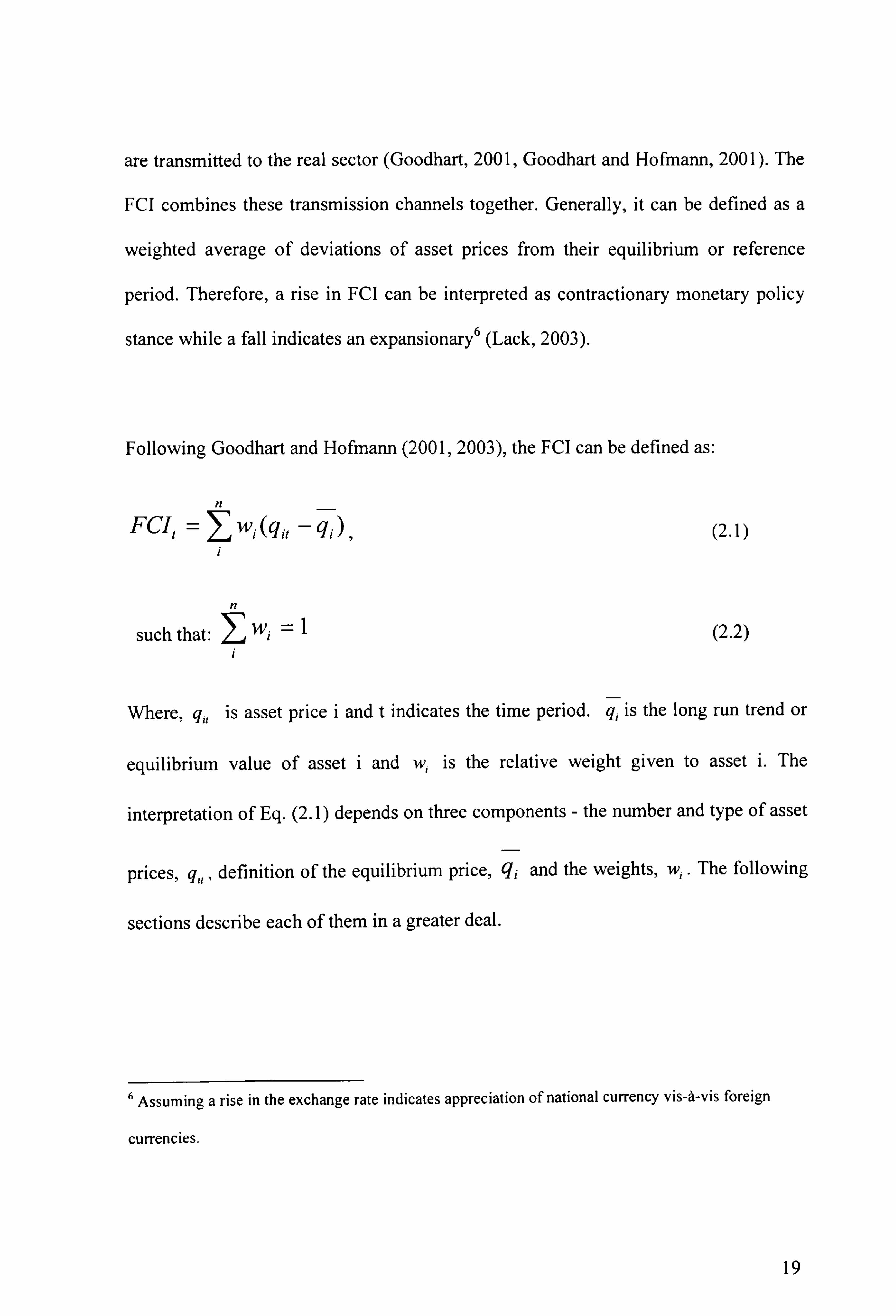
are transmitted to the real sector (Goodhart, 2001, Goodhart and Hofmann, 2001). The
FCI combines these transmission channels together. Generally, it can be defined as a
weighted average of deviations of asset prices from their equilibrium or reference
period. Therefore, a rise in FCI can be interpreted as contractionary monetary policy
stance while a fall indicates an expansionary 6 (Lack, 2003).
Following Goodhart and Hofmann (2001,2003), the FCl can be defined as:
n
FCII w, (qi, - qj),
n
such that: Wi (2.2)
Where, q,, is asset price i and t indicates the time period. q, is the long run trend or
equilibrium value of asset i and w, is the relative weight given to asset i. The
interpretation of Eq. (2.1) depends on three components - the number and type of asset
prices, q, definition of the equilibrium price, qj and the weights, w,. The following
sections describe each of them in a greater deal.
Assuming a rise in the exchange rate indicates appreciation of national currency vis-A-vis foreign
currencies.
19
Page 32
2.2.3 The use of variables in an FCI
A survey of the literature presented in Table 2.1, shows that the real interest rate and
the real exchange rate are commonly used in the construction of the MCI. Besides the
MCI variables, Goodhart and Hofmann (2001,2003) and Mayes and Viren (2001)
include real house prices and real share prices in the construction of the FCI for
Europe, USA and Japan. On the other hand, Lack (2003) constructs FCls for
Switzerland using only three variables - the real interest rate, the real exchange rate
and the real house price. Gauthier et al. (2004) obtain a broad based FCI for Canada.
They include long-term interest rates and the corporate bond risk premium in addition
to the four variables proposed by Goodhart and Hofmann (2001,2003).
Instead of using house prices and share prices, there is also a practice of using
alternative financial variables to represent the credit and balance sheet channels. For
instance Macroeconomic Advisors (1998) use the dividend price ratio and household
equity wealth. Carmichael (2002) and Goldman and Sachs (2000) include the yield
curve and the money supply as financial variables in their Ms.
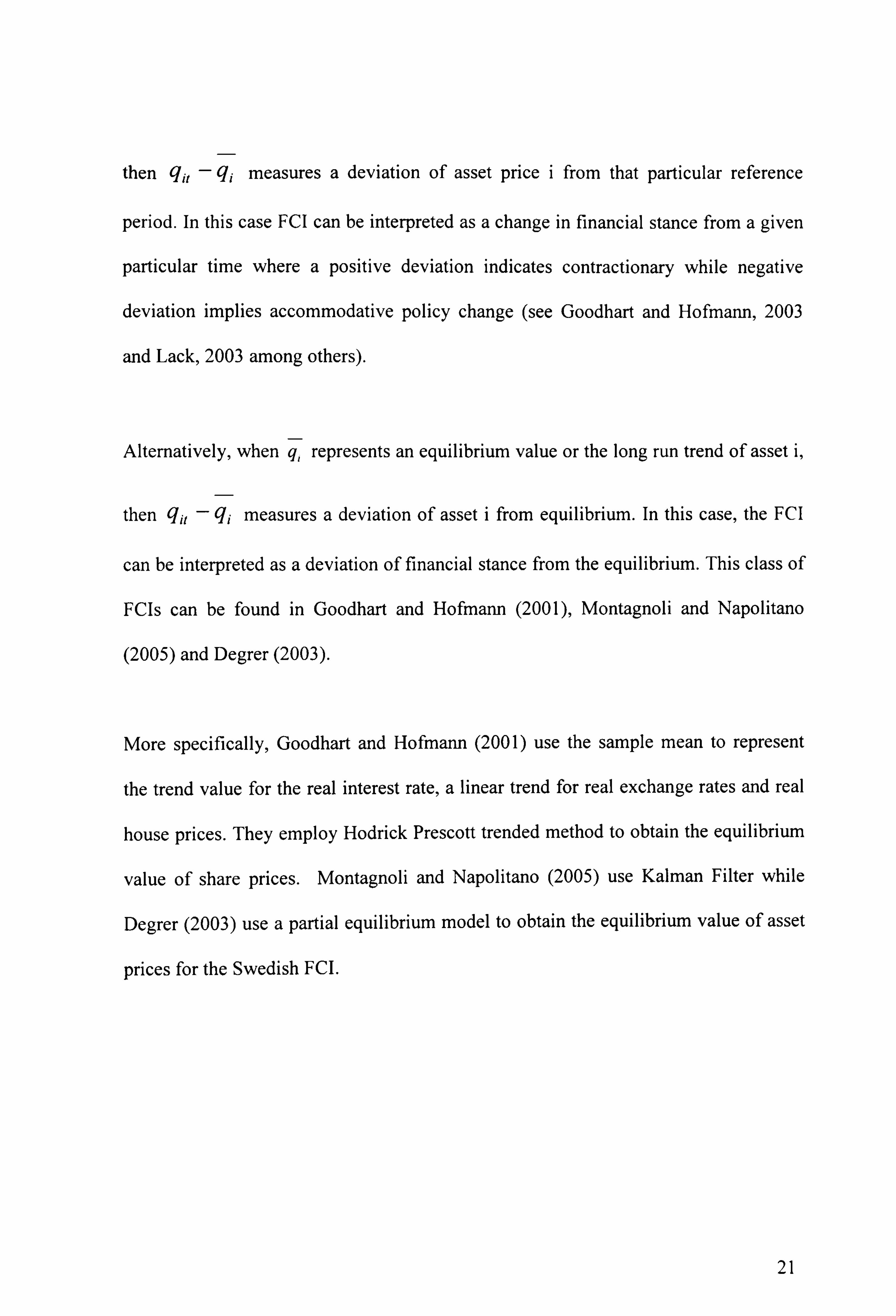
2.2.4 Defining equilibrium asset prices
The literature offers two types of interpretations of an FCI depending upon the
definition of q, . When q, is defined as the value of any reference period of asset i,
20
Page 33
then q,, - q, measures a deviation of asset price i from that particular reference
period. In this case FCI can be interpreted as a change in financial stance from a given
particular time where a positive deviation indicates contractionary while negative
deviation implies accommodative policy change (see Goodhart and Hofmann, 2003
and Lack, 2003 among others).
Alternatively, when q, represents an equilibrium value or the long run trend of asset i,
then q,, - q, measures a deviation of asset i from equilibrium. In this case, the FCI
can be interpreted as a deviation of financial stance from the equilibrium. This class of
FCls can be found in Goodhart and Hofmann (2001), Montagnoli and Napolitano
(2005) and Degrer (2003).
More specifically, Goodhart and Hofmann (2001) use the sample mean to represent
the trend value for the real interest rate, a linear trend for real exchange rates and real
house prices. They employ Hodrick Prescott trended method to obtain the equilibrium
value of share prices. Montagnoli and Napolitano (2005) use Kalman Filter while
Degrer (2003) use a partial equilibrium model to obtain the equilibrium value of asset
prices for the Swedish FCI-
21
Page 34
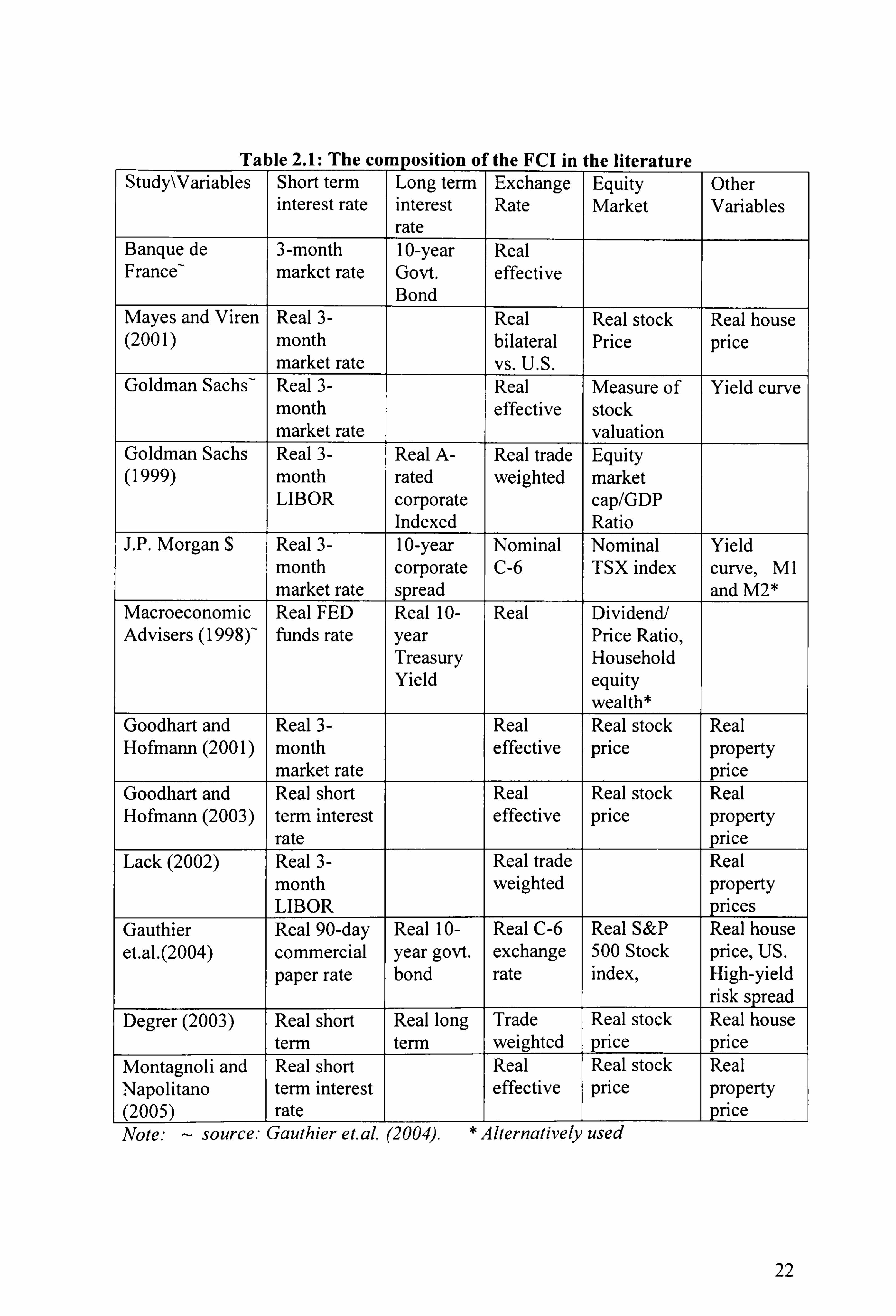
Table 2.1: The comnosition of the FCI in the literature Study\Variables Short term Long term Exchange Equity Other
interest rate interest Rate Market Variables rate
Banque de 3-month I 0-year Real France- market rate Govt. effective
Bond Mayes and Viren Real 3- Real Real stock Real house (2001) month bilateral Price price
market rate vs. U. Sa Goldman Sachs- Real 3- Real Measure of Yield curve
month effective stock market rate valuation
Goldman Sachs Real 3- Real A- Real trade Equity (1999) month rated weighted market
LIBOR corporate cap/GDP Indexed Ratio
J. P. Morgan $ Real 3- 1 0-year Nominal Nominal Yield month corporate C-6 TSX index curve, MI market rate_ spread and M2*
Macroeconomic Real FED Real 10- Real Dividend/ Advisers (1998)- funds rate year Price Ratio,
Treasury Household Yield equity
wealth* Goodhart and Real 3- Real Real stock Real Hofmann (2001) month effective price property
market rate price Goodhart and Real short Real Real stock Real Hofmann (2003) term interest effective price property
rate price Lack(2002) Real3- Real trade Real
month weighted property LIBOR prices
Gauthier Real 90-day ReallO- Real C-6 Real S&P Real house et. al. (2004) commercial year govt. exchange 500 Stock price, US.
paper rate bond rate index, High-yield risk spread
Degrer (2003) Real short Real long Trade Real stock Real house term term weighted price price
Montagnoli and Real short Real Real stock Real Napolitano term interest effective price property (2005) rate price Note: - source: Gauthier et. al. (2004). * Alternatively used
22
Page 35
Contd Study\Variables FCI Variables modelled as Sources of FCI Weights
constructed for
Banque de G-7 Change from a base IMF's and OECD's France- countries period Macroeconomic model Mayes and Viren 17 countries Level of real interest rate IS curve (single (2001) and exchange rate; first equation)
difference of the rest Goldman Sachs- Canada Unknown Simple average Goldman Sachs USA Deviations from historic FED macro model (1999) mean J. P. Morgan $ Canada Deviation from mean Simple average
divided by variance Macroeconomic USA Not specified: referred to Washington University Advisers (1998)- as "technical adjustment" Macro model Goodhart and G-7 Deviation from trend: 1. reduced form IS and Hofmann(2001) countries long run mean for interest Philips curve model.
rate, linear trend for 2. Impulse functions of a exchange rate and house VAR*
prices; and HP filter for
stock price Lack(2002) Switzerland First difference of Shocks to restricted and
variables structural macro model* Goodhart and USA, UK, Level for real interest rate Single equation IS curve Hofmann (2003) Japan, EU and real exchange rates
and first difference for house and share prices
Gauthier et. al. Canada First difference and HP Single equation (IS (2004) filtered* curve), VAR generalized
impulse response function and factor
analysis" Degrer (2003) Sweden Partial estimate of each VAR impulses
variable Montagnoli and USA, UK, Kalman Filter Single equation IS curve Napolitano (2005) Canada, EU Note: - source: Gauthier et. al. (2004). two scenarios are presented
S Source: Carmichael (2002) **. - Three scenarios calculated
23
Page 36
2.2.5 Weigh calibration process
There are at least five methods to obtain weights for asset prices, w, (see Goodhart
and Hofmann, 2000 and Gauthier et al. 2004). They are:
Simulation of a large-scale macroeconomic model
Small scale macroeconomic models
Aggregate demand model
VAR impulses-response function
Factor analysis
Large scale macroeconomic models capture the structural features of the entire
economy. Goldman and Sachs (1999) and Macroeconomic Advisers (1998) use such a
large-scale model to obtain weights for FCl components. Although a large-scale model
incorporates all necessary information while predicting weights, the literature argues
that they are less useftil in practice for two reasons. First, Gauthier et al. (2004) argue
that stock prices and share prices play a limited role in many large-scale macro models
currently used by central banks so that weight generation from this process may
underestimate the actual role play by these variables in the economy. Second,
Goodhart and Hofmann (2001) believe that a large-scale macro model with an explicit
role for property price is still unavailable.
24
Page 37
The second option is to employ a small-scale macroeconomic model. A typical small-
scale macroeconomic model consists of a Philips curve and an IS curve. Following
Goodhart and Hufffiann (2001) and Gauthier et al. (2004), a simple macroeconomic
structural model can be written as:
nn
k, + ki; r, -, +I j=l
(2.3)
mmmmm b, + lby,
-, + 1] a, r, -, + Ea,, e, -, + lahjh,
-j+Za, s, +c, (2.4) -j i=l j=l J=j J=j j=l
Equation (2.3) is the Philips curve and (2.4) is the IS curve where ;r is inflation, y is
the output gap, r is the real interest rate, e is the real exchange rate, h is the real house
price index, and s is the real share price index. The last variable of each equation is
the error term which is assumed to be mutually uncorrelated with zero mean and
constant variance and finally other remaining terms are unknown parameters to be
estimated.
In this framework, the relative weights, W, , which appear in the construction of an
FCI, can be written as:
25
Page 38
J]m a W, = Im
J=l y for 1 == {r, e, h, s) (2.5)
-. 4 a+ Im a+ J', a,, + fn a J=j ri , J=l ej j= J=l si
One of the criticisms of this approach is that it assumes the closed economy Philips
curve that excludes the direct impact of exchange rate on inflation. Ball (1999),
Guender (2001 a) and Guender and Matheson (2002) argue that changes in the real
exchange rate should be included in the Philips curve to measure the direct impact of
exchange rates.
The third and most commonly used approach is to derive the FCI weights from the IS
curve, i. e. Eq. (2.4). This approach explicitly believes that inflation solely depends on
the output gap. Goodhart and Hofmann (2003) and Mayes and Viren (2001) generate
FCI weights while Duguay (1994), Mayes and Viren (2000), among others, compute
MCI weights based on this approach. It is, however, argued that FCI weights obtain
from this model may not reflect the economic conditions as it potentially neglects the
supply side of economy (eg. Guender and Matheson, 2002).
The fourth method given in the literature is the vector auto-regression (VAR)
estimation. Initially, Goodhart and Hofmann (2001) and later on Gauthier et al. (2004)
explore the reduced-form approach to a VAR technique. Under this method, they
obtain alternative weights of all asset prices based on the impulse responses of
26
Page 39
inflation to asset price shocks in an identified VAR. They identify the shocks using a
standard Cholesky factorization with ordering output gap, inflation, real house prices,
real exchange rate, real interest rate and real share prices.
Finally, the other option in developing an FCl is a liner weighted combination of
financial variables through the factor analysis. It extracts weighted liner factor from a
numbers of variables which is suppose to detect common structure and remove 'noise'
created by irregular movements. Watson (1999) and Gauthier et al. (2004) use this
technique as an alternative to VAR impulse and the reduced form models.
2.2.6 The use of the FCI in monetary policy
The FCI can be used in a number of different ways. Goldman and Sachs (1999) and
Macroeconomic Advisers (1998) use it to predict inflation and output growth several
quarters ahead and to predict the future course of monetary policy. Goodhart and
Hofmann (2001,2003) find that the FCl can be used as a leading indicator to predict
inflation and output as it contains useful information about future inflation. Gauthier et
al. (2004) argue that when there are shocks to the economy, changes in the FCI may
provide an indication of the markets' reactions and expectations regarding ftiture
monetary policy. They further write "the FCI can be used as a synthetic measure of the
financial conditions that economic agents face and thus constitutes a broad assessment
of the financial stance. "
27
Page 40
More specifically, the FCI can be used in two different ways in the conduct of
monetary policy - as an important informative variable or as an operational target.
Under the first approach, the FCI enters in a monetary policy reaction function so that
central bank not only responds to deviations of inflation from the target and to the
output gap but also to the FCI. This approach can be found in Montagnoli and
Napolitano (2005) who find that FCI-augmented Taylor Rule outperforms the simple
Taylor rule.
The FCI can also be used as a policy rule. Goodhart and Hofmann (2001,2003) argue
that the optimal monetary policy reaction function is such that the interest rate should
not only react to inflation and output gap but also to the real exchange rate, real house
prices and real share price. Under this option, policyrnakers aim to keep FCI at a par
by changing short-term interest rates in order to minimise adverse effects of asset
prices to the output gap and inflation. This framework is similar to the MCI rule that
has been used by the Bank of Canada, with a few other central banks, as intermediate
target since early 1990s (Freedman, 1994, Duggay, 1994).
The FCI is, however, a recently developed approach to deal with a broader view of
monetary policy but never been tested as an operational target or any type of policy
rule by the central banks. Although it contains important information for predicting
inflation and output, it has been criticised on two grounds. Firstly, it is model
28
Page 41
dependent and robust estimation including the issues of parameter inconsistency,
dynamism, and non-exogeneity never been conducted properly, which limits the scope
of applicability (Eika et al. 1996, Ericsson et al. 1996 and Gerlach and Smets 2000).
Secondly, Bernanke and Gertler (1999) and Gertler et al. (1999) oppose using the FCl
as a policy variable. They argue that monetary policy would be more volatile if central
banks use FCI as a policy variable due to uncertainty and a high volatility contained in
share prices and house prices.
2.3 Financial conditions index: a theoretical formulation
In this section, we propose a theoretical framework where the FCI weights can be
obtained from a macroeconomic structural model. The model consists of an open
economy Philips curve, an open economy IS curve and the UIP. After formulating the
structural model, we then define two types of inflation targeting framework, strict CPI
inflation and domestic inflation targeting, as an objective of monetary policy. Finally,
we combine each policy objective with the structural model to obtain an optimal
monetary policy reaction function with appearing an FCI.
29
Page 42
2.3.1 Structural model
We use a small scale macroeconomic model to obtain the optimal monetary policy
reaction function. This model assumes an open economy where the exchange rate is
assumed to be flexible.
The structural model consists of three equations, a Philips curve, an IS curve and the
UIP as:
g, = (e, -, - e, -2
)+ 17,
YI -ß r, -, -'52e, -, +, ý2y,
-, - 0, z�, -,
rt --.,: rf - (E, e,,, - e, )+p,
(2.6)
(2.7)
(2.8)
Where, ; r, is the CPI inflation, y, is the output gap (i. e the difference between actual
and potential output), e, is the real effective exchange rate (REER)7, z,, is the
financial variable, r, is the domestic real interest rate, rf is the foreign real interest
rate, and E, e, +, is the expectation formed at time t for the real exchange rate at time
t+1 .
an increase in e, denotes an appreciation of home currency vis-a-vis foreign currencies.
30
Page 43
q, and c, are random shocks to inflation and output respectively. They are assumed to
be mutually uncorrelated with zero mean and constant variances. Finally, p, is defined
as the time varying premium. For simplicity, constants are normalized to zero and all
variables except interest rate are measured in logs.
Eq. (2.6) is a standard open-economy Phillips curve as used by many authors (for
instance Ball, 1998 and Guender and Matheson, 2002 amongst others). It describes
that changes in current inflation depends on its own lag, the output gap, lagged
changes in the real exchange rate as well as a supply shock.
Following Ball (1998), Goodhart and Hofmann (2003), we define an open economy IS
curve in Eq. (2.7) where the output gap depends on lags of the real interest rate, lags of
the real exchange rate, its own lag, lags of financial variables and a demand shock.
Depending upon the state of the economy and the effectiveness of monetary policy,
financial variables can be any combinations of equity and property prices as proposed
by Goodhart and Hofmann (2003) or the long term interest rate and financial ratios as
proposed by Kennedy and Riet (1995).
We introduce uncovered interest parity (UIP) in Eq. (2.8). Following Ball (1998) we
believe that the UIP condition does not hold perfectly so that a time varying
premium, p, , plays a role in the model.
31
Page 44
2.3.2 Inflation targeting
Following Taylor (1993), a large bulk of literature assumes that policyrnakers aim to
minimize the variability of inflation and the variability of real output from their
respective targets. This type of policy setting provides a trade off between inflation
and output.
We consider a special case of this framework where inflation targeting is considered to
be the only objective of monetary policy (Guender and Matheson, 2002 and Ball,
1998). Further, we specify the role of the real exchange rate within the inflation
targeting framework as it has twin effects on inflation. It affects directly through the
import price channel and indirectly through the effects on aggregate demand (see
Bernanke et al., 1999 and Ball 1999 for more discussion).
In order to address this issue in the conduct of monetary policy, we consider two types
of inflation targeting frameworks, namely, strict CPI inflation targeting and domestic
inflation targeting. In the former case, imported inflation is included in the
measurement of the CPI, implies that the monetary authority does not consider the
direct effects of the REER separately. In the latter case, however, the authority
considers the domestic inflation and the import price separately.
32
Page 45
We first derive an optimal monetary policy reaction ftinction for the CPI inflation
targeting and then consider the domestic inflation targeting. Under both frameworks,
we obtain the optimal monetary policy reaction function in terms of the FCl-
2.3. Z 1. Strict CPI inflation targetingframework
Following Guender (2001a, 2001b), Guender and Matheson (2002) and Ball (1998)
among others, we assume that policyrnakers announce a strict target for CPI inflation
for the two periods ahead:
; r*= Elgt+2 ýo (2.9)
Where, ; T* is the inflation targeted rate, E, 7rt+2 is the expectation formed at time t of
CPI inflation at time t+2.
To construct the optimal reaction function, we update Eq. (2.6) by two periods and
take conditional expectations; yields,
EIZI+2 ,,,: E, irt+l + 2,1 E, y, +j - (51 (E, e, +, -
substituting Eq. (2.10) into (2.9) and rearranging the terms results in:
(2.10)
33
Page 46
E, e, +, -e, =I (E, 7r, +, +, ý, jEly, l) 91
Now, replacing Eq. (2.11) into (2.8), we get:
(51 (rf - r, )=E, 7r,,, + 11 E, y, +1 + p, (2.12)
Again, updating and taking expectations in Eq. (2.6) and (2.7) results in:
EI 7r, +, : -- 71 +ýy, - 9, (e, - e, -,
) (2.13)
EtYI+l = -ß r, -'52e, +'ý2Y, - OZI (2.14)
Substituting Eq. (2.13) and (2.14) into (2.12) and re-arranging terms with
appearing r, , e, and z, on left hand side, yields:
'U, r, + lU2e, + ZDr3Z, = 7r, +(5, e, -, +. ý, (1 +'ý2)yl - Olfif + Pt (2.15)
where,
lul = 46 -. 51 (2.16)
ZU2 = 'ý t52 + t5l (2.17)
ZU3 = 'ýlo (2.18)
34
Page 47
Eq. (2.15) is the optimal monetary policy reaction function with an FCl components (r,
e, and z) on the left hand side where mr, (for i= I to3) are coefficients of the real interest
rate, the real exchange rate and the financial variable respectively.
89 Finally, we rescale v7i by dividing /ý (, 6+62+0)
, we get,
vyi (for i=I to 3) 21 (18 + 452 + 0)
Where, Wi is the relative weight of asset i
As stated, our model is flexible in nature as we can add or remove any asset prices in
the FCI framework depending on their relevancy to the economy. On the other hand, if
we exclude asset prices from the model, i. e. when z=O, the model reduces to the MCI,
which can be written as
V, r, +V2e, = 7r, +i5, e, -, +'ý, (1 + A2)YI - 131fif +A
where,
V, = 48 - . 51
V2 :- 'ý t52 + 451
8 The reason for re-scaling coefficients is given in section 2.
Which is the sum of the coefficients of asst prices, i. e. r17, + 02 + 173
(2.20)
(2.21)
(2.22)
35
Page 48
(for i=I to 2) (2.23) 'ýl (18 + '52 )
Eq. (2.20) is an optimal reaction function with appearing an MCI on the left hand side
leaving right hand side unchanged.
2.3. ZZ Domestic inflation targetingframework
In the CPI inflation targeting framework, the condition 1ý, 8 > . 5, must be satisfied in
Eq. (2.16) and (2.2 1) in order to get a valid interpretation of the model. Any violation
produces a paradoxical result and the model becomes unstable.
This situation may arise if there is a heavy pressure of import prices on CPI. In this
context, we argue that policyrnaker should consider the domestic inflation and the
imported inflation (i. e. exchange rate) separately in order to identify this problem.
Therefore, following Ball (1999) and Guender and Matheson (2002) we modify the
objective function as given by Eq. (2.9) as follows:
z*= El'71+2 + 91 (E, e�, - e, ) =O (2.24)
Eq. (2.24) depicts the domestic inflation targeting framework where the term E, 7r, +2 is
the expectation formed at time t of domestic inflation at time t+2. The parameter 5, is
36
Page 49
an escalating factor which measures the direct impact of expected change in the real
exchange rate on inflation.
In the extreme case, when i5l =0, there would be no difference between the CPI
inflation targeting and domestic inflation targeting frameworks, indicating that there is
no direct role of the change in the real exchange rate on inflation. On the other
extreme, when 15, =1, there would be a proportional relationship between the change in
the real exchange rate and inflation, indicating that the inflation is overwhelmingly
determined by the exchange rate. We consider 51 such that 0<, 5, <1.
In the process of formulating the optimal reaction function, we substitute Eq. (2.24)
into (2.10), which results in:
El; rl+l + /ý E, y,,, = (2.25)
Now, inserting Eq. (2.13) and (2.14) into (2.25) and rearranging the terms we obtain
the optimal monetary policy reaction function with appearing an FCl on the left hand
side as:
0), r, + 0)2e, + (t)3 Z, = '7, +9, e, -, + /ý
(1 + A2 )yt
where w, = 21,8
0)2 = 'ý (52 + 451
(2.26)
(2.27)
(2.28)
37
Page 50
Ct)3 --": 'ýl
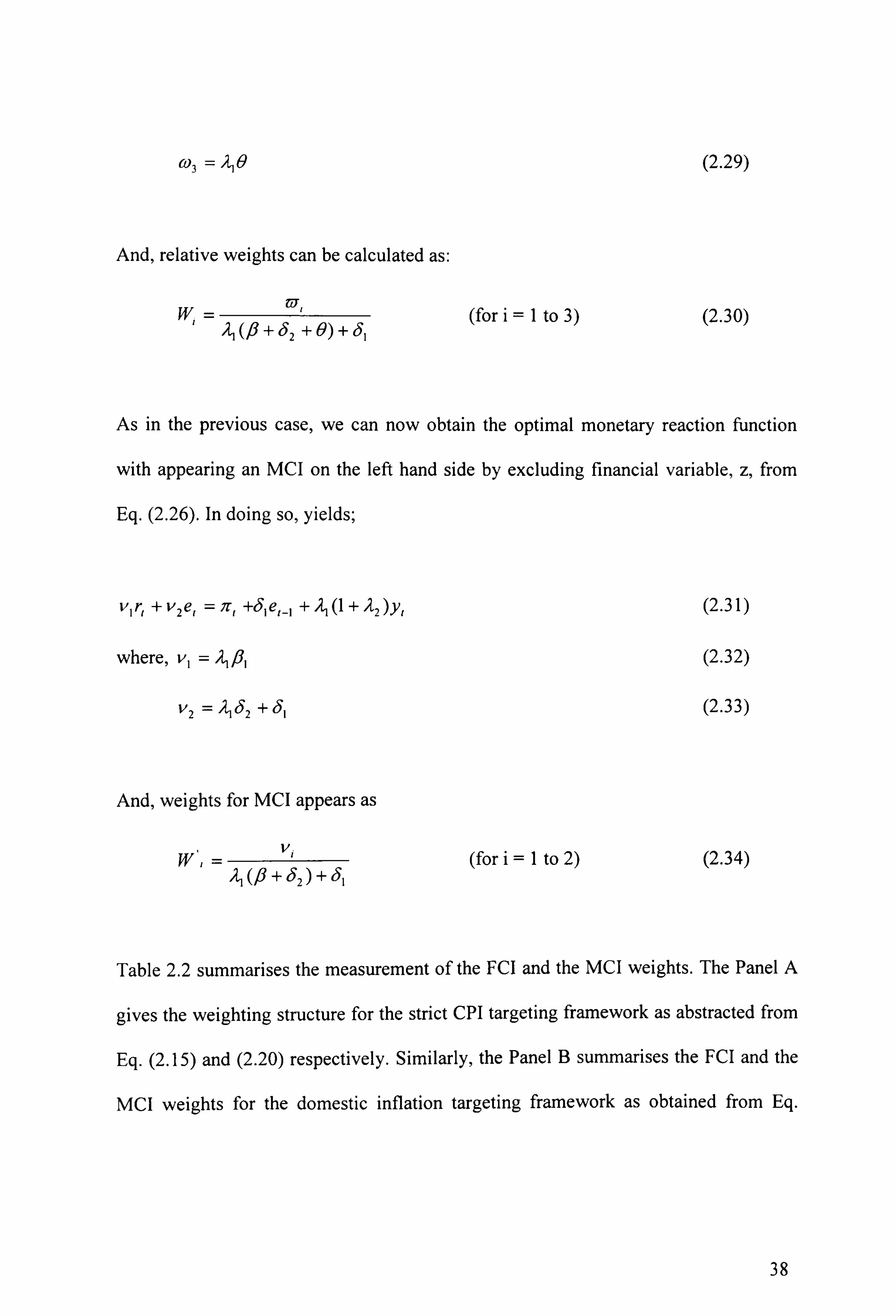
And, relative weights can be calculated as:
zu, (for i=I to 3) 'ýl (18 + 452 + 0) + t5l
(2.29)
(2.30)
As in the previous case, we can now obtain the optimal monetary reaction function
with appearing an MCI on the left hand side by excluding financial variable, z, from
Eq. (2.26). In doing so, yields;
V, r, + V2 e, = 7r, +15, e, -,
+ 21 (1 + 'ý2 )YI
where, v, = ýjflj
V2 'ýl 62 + 151
And, weights for MCI appears as
VI
(18 +52) +'51 (for i=I to 2)
(2.31)
(2.32)
(2.33)
(2.34)
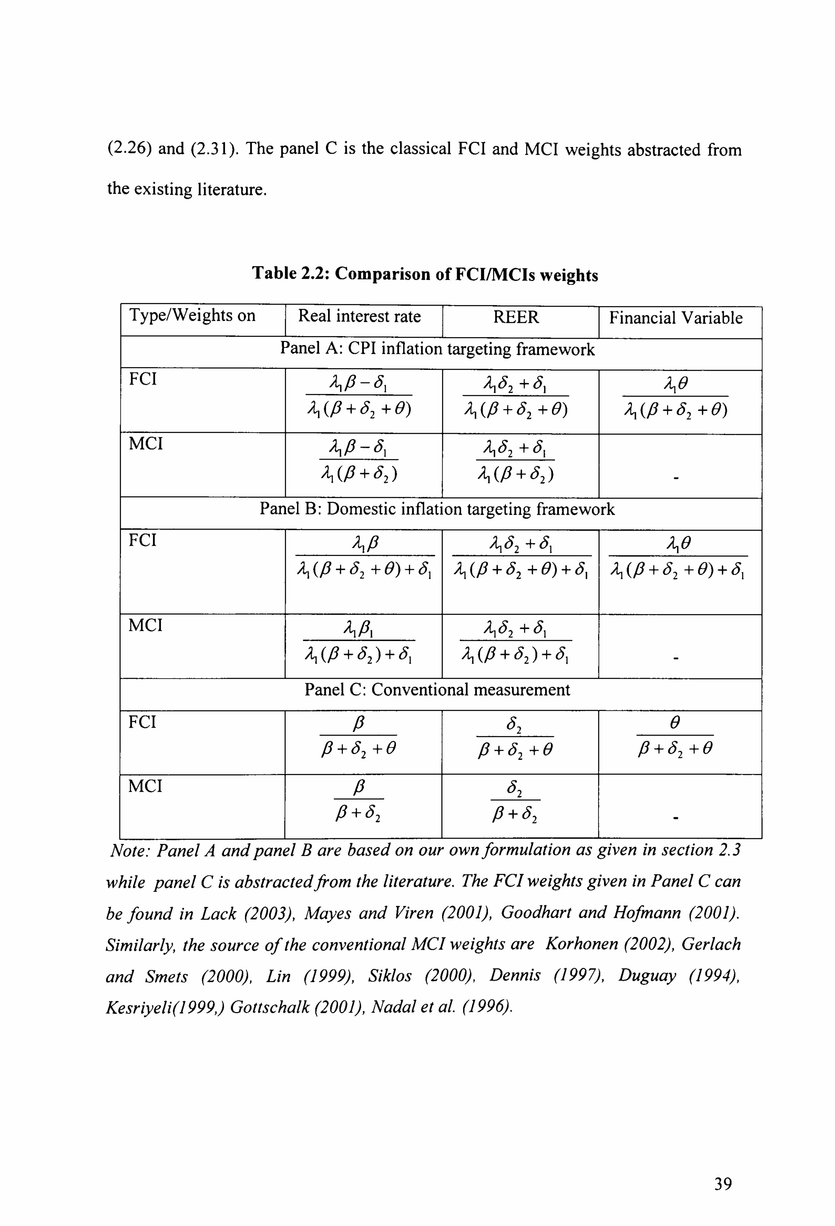
Table 2.2 surnmarises the measurement of the FCI and the MCI weights. The Panel A
gives the weighting structure for the strict CPI targeting framework as abstracted from
Eq. (2.15) and (2.20) respectively. Similarly, the Panel B summarises the FCI and the
MCI weights for the domestic inflation targeting framework as obtained from Eq.
38
Page 51
(2.26) and (2.31). The panel C is the classical FCI and MCI weights abstracted from
the existing literature.
Table 2.2: Comparison of FCI/MCIs weights
Type/Weights on Real interest rate ---- T REER T Financial Variable
Panel A: CPI inflation targeting framework
FCI ý1)6 - t5l /ý 452 + 451 0
2168 + 62 + 0) 'ýl 68 + 452 + 0) 'ýl (18 + '52 +0)
MCI 21)6 -15, 'ýl
G8 + '52
ý1 t52 + 61
ý1 (16 + 452
Panel B: Domestic inflation targeting framework
FCI 46 'ýl 452 + 461 210
'ýl (8 + 452 + 0) + 461 'ýl
0+ 452 + 0) + 451 'ýl (18 + 452 + 0) + 451
MCI ý, 61 'ý 62 + '51
Al (6 + t52) + (51 66 + t52) + (51 -
Panel C: Conventional measurement FCI P
+ (52 +0
(52
)6+t52 +0
0
)6+(52 +0
MCI
-J6 P+ t52
152
16+(52
Note: Panel A and panel B are based on our own jormulation as given in section 2.3
while panel C is abstractedftom the literature. The FCI weights given in Panel C can
be found in Lack (2003), Mayes and Viren (2001), Goodhart and Hofmann (2001).
Similarly, the source of the conventional MCI weights are Korhonen (2002), Gerlach
and Smets (2000), Lin (1999), Siklos (2000), Dennis (1997), Duguay (1994),
Kesriyeli(I 999, ) Gottschalk (2001), Nadal et al. (1996).
39
Page 52
Comparing panel A and B with panel C, we can observe that our indices are
improvement over the existing literatures for two reasons. Firstly, in our framework,
the relative weights of asset prices are obtained from a structural model which
combines both the IS and the Philips curve as compared to the IS curve alone on the
existing literature.
Secondly, our FCI weights take an account of both the direct and indirect effects of the
changes in the real exchange rates where the direct effect transmits through S, and
indirect effect through 82 . The existing literature, on the other hand, excludes 9, in the
FCI weights.
2.4 Empirical estimates of the financial conditions index
2.4.1 Data generating process and unit root test
We consider two open economies, the UK and the USA, for our empirical analysis.
As monthly GDP series is not available, we use quarterly time series data for both
countries. The sample period covers from 1979QI to 2003Q4. Following Goodhart
(2001) we use the real interest rate, r, the real effective exchange rate, e, real house
40
Page 53
prices, h, and real share prices, s, in the construction of Ms. We use logs of all
variables except for the interest rate' 0
We use real GDP as the measure of output and employ the Hodrick-Prescott filter with
smoothing parameter set at 1600 to obtain potential output. The output gap, y, is then
measured by subtracting potential output from the actual. The real interest rate, r, is
obtained by subtracting inflation, 7r, from the nominal interest rate , R. 71 is calculated
as the percentage change in the consumer price index over the same quarter of the
previous year. We use the real effective exchange rate (REER) as a measure of the
exchange rate, where an increase indicates appreciation of home currency vis-A-vis
foreign currencies. The sources and definitions of variables are given in Appendix 2.1.
We next run the augmented Dickey-Fuller (Dickey and Fuller, 1979) and Phillip and
Perron (1988) tests to test the stationary of our variables (See Appendix 2.2 for the
detailed methodology). Both tests the null hypothesis of a unit root but the procedure
is a little different. While the fon-ner test makes a parametric correction for higher-
order correlation by assuming that the series follows an auto-regressive process with
order ar(p) and adjusts the test methodology by adding lags of independent variables,
10 However, the distribution of the US and the UK interest rate are asymmetric around their mean
because the skewness for the US and UK interest rates are found to be 0.90 and 0.26 respectively. On
the other hand, the US interest rate is peaked whereas the UK interest rate is flat relative to the normal
as the kurtosis of the US and UK interest rates are recorded to be 3.74 and 1.88 respectively.
41
Page 54
the PP method tests the unit root through a non-parametric correction procedure
(Banerjee et al., 1993).
Table 2.3: ADF test (1979Q1 to 2003Q4)
Variables Y, g/ -; T T R, e, SI h,
Panel A: UK
Level -1.01 -3.52* -2.91 -2.17 -0.97 -2.38 First Difference -4.08* -5.21 * -3.58* -4.12* Deviations from the
equilibrium#
-3.96* -5.17* -4.98* -4.68*
Panel B: USA
Level -0.14 -3.88* -3.01** -1.13 -0.14 -0.12 First Difference -3.18* -3.98* -4.42* -3.01 **
Deviations from the
equilibrium#
-3.88* -5.61 -3.77* -3.53*
Note: 1. Mackinnon critical valuesfor the rejection of the null hypothesis at 1%, 5%
and 10% are -3.49, -2.89 and -2.59 respectively.
2. # Equilibrium values are obtained using the Hodrick-Prescott (1977)filter.
3. Data source and definition of variables are given in Appendix 2.1
4. * and ** indicate significant at I% and 5% respectively.
Table 2.3 shows the test results. We find similar results from both the ADF and PP
tests so we only report the ADF test to save space. We find inflation, output gap and
the real interest rate to be 1(0) while house price, share price and the real exchange rate
indices to be l(l) process.
42
Page 55
2.4.2 Estimation and interpretation
In this section, we first estimate the structural model given by section 2.3.1 and then
compute the FCI and MCI using the formulae given in Table 2.2.
Table 2.4 reports the OLS estimates of the open economy Philips curve, that is Eq.
(2.6), for the UK and the USA. The lag length is chosen using a general to specific
approach starting from 9 lags, but the best estimate is obtained when using up to five
lags of the dependent variable for both countries.
Both estimates are well specified. The DW statistics reject the null of a unit root whilst
Godfrey's (1988) Lagrange Multiplier (LM) test suggests that there is no
autocorrelation in the residuals. Moreover, no functional form misspecification is
detected by the Ramsey's (1969) RESET test and the non-normality of the estimate is
rejected by Jarque-Bera's (1980) test. Evidence of homoscadesticiy is clearly
established. Also, no signal of auto regressive conditional heteroscadesticity appears
both from the first order and up to fourth order condition. Finally, our estimates pass
CUSUM and CUSUMQ tests, indicating that the estimates are stable.
Our results are in line with the existing empirical findings for both countries as
inflation has a positive relationship with the output gap and an inverse relationship
with the REER. The effect of the real exchange rate on inflation in UK is higher than
43
Page 56
that of the USA. The change in the oil price is also found to be significant at 5% for
both countries.
Table 2.4: Philips curve estimates
[Model: ir, = ; rl-I + /ý y, -, + 5, Ae,
-, + 77,1
Estimated Parameters \ Country
(lag length of the dependent variable)
UK
(1-5)
USA
(1-5)
0.250 (0.039)* 0.171 (0.056)*
(51 -0.027 (0.009)* -0.013 (0.005)**
AOP 0.015(0.008)** 0.017(0.007)**
Diagnostic statistics/tests
Adjusted R' 0.94 0.95
Durbin-Watson statistics 1.74 1.72
Standard error of regression 0.43 0.56
Jarque-Bera statistics for normality test 3.01 [0.18] 4.29 [0.12]
Breusch-Godfrey serial correlation LM(l) 0.98 [0.32] 2.15 [0.14]
Breusch-Godfrey serial correlation LM(4) 1.26 [0.29] 1.47 [0.23]
ARCH 1 0.04 [0.83] 1.56 [0.21]
ARCH 4 1.72 [0.15] 2.01 [0.11]
White's heteroskedasticity test 1.73 [0.13] 2.09 [0.06]
Ramsey's RESET test 1.49 [0.33] 1.03 [0.30]
Chow's breakpoint test 1.16 [0.34] 2.12 [0.10]
Note:
(a) AOP is the coefficient of the change in the oil price. Notice that this variable
is not included in (2.5) to make the model simpler but included in the
empirical estimations to get more robust results (see Goodhart and
Hofmann, 2003for the similar experiment).
44
Page 57
(b) Sample periodfor UK and USA are 1980QI-2003Q3 and 1979Q3-2003Q4
respectively. (c) Constant and lags of dependent are also included in the estimates but is not
reported to save space, is available on request. (d) is the standard error and [] is the probability of the test statistics. (e) ** and *** indicate significant at 1%, 5% and 10% respectively.
Chow's breakpoint is 1992. Q4 and 1987. Q3 for the UK and USA
respectively.
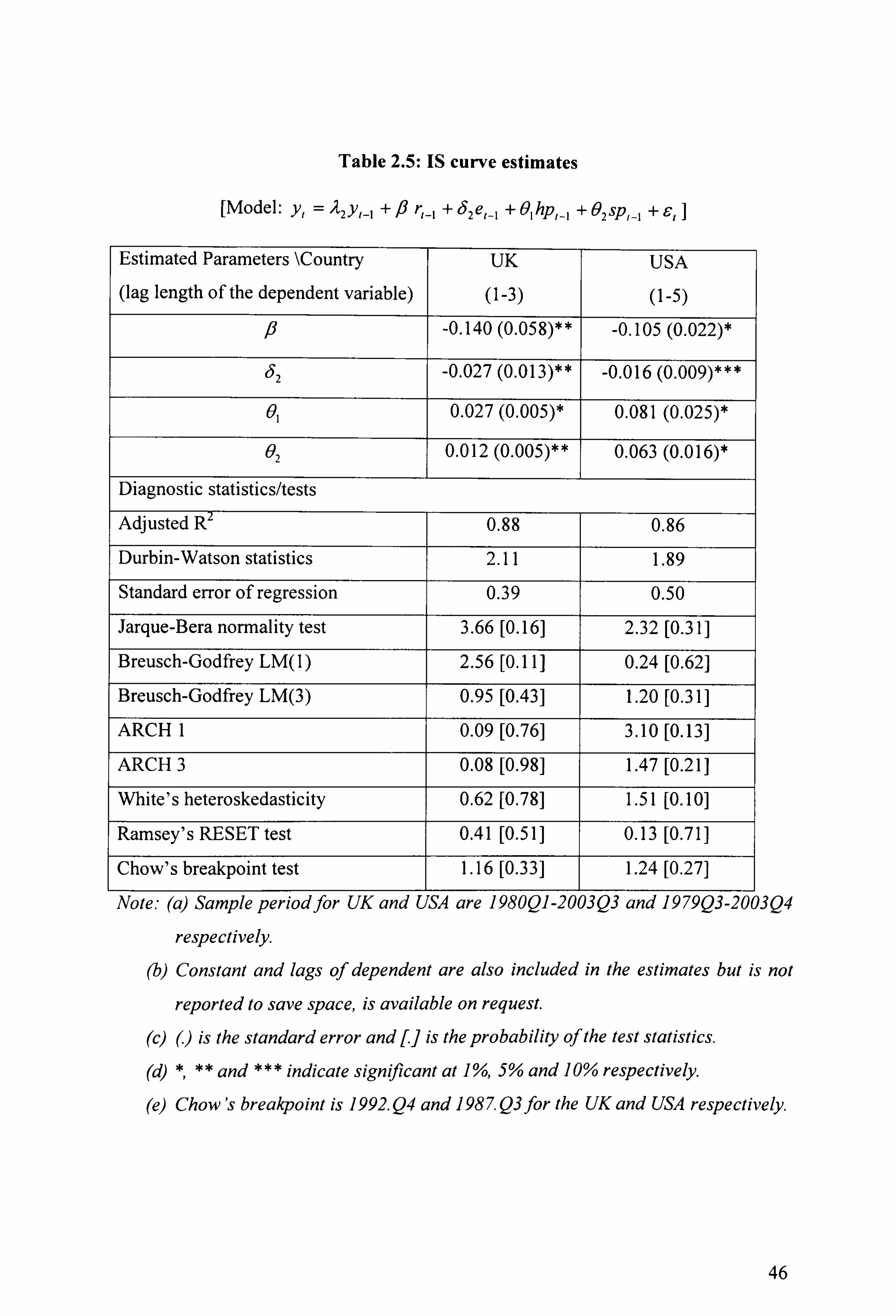
Next, we estimate the IS curve for the UK and the USA, that is Eq. (2.7). Table 2.5
reports the empirical estimates. We find that the real interest rate and the REER have a
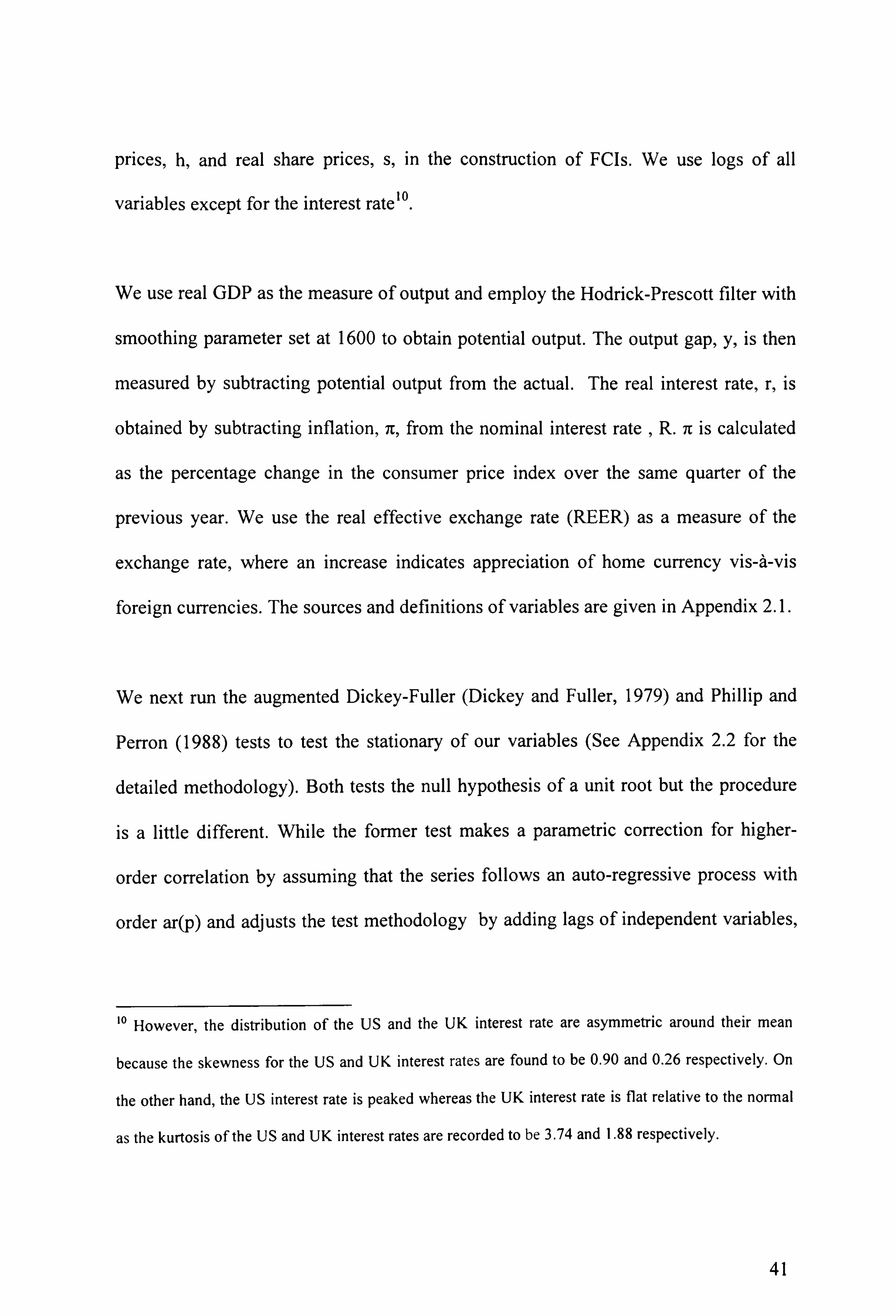
negative impact while real house prices and real share prices have a positive impact on
the output gap. The size of the estimated coefficients show that the real interest rate
has a greater impact on the output gap in USA followed by real house prices, share
prices and the REER. However, the REER and real house prices have a similar impact
on the output gap in UK after the real interest rate.
Using the methodology given in Table 2.2 and the estimated coefficients from Tables
2.4 and 2.5, we now obtain the weights on real interest rates, REER, real house prices
and real share prices for the construction of FCI. Notice that the financial variable, z,
as discussed in our theoretical model comprises real house prices and real share prices
in our empirical analysis. Therefore, we replace 0 by 01 and 02 in Table 2.2 in order to
get separate weights of these variables.
45
Page 58
Table 2.5: IS curve estimates
[Model: Y, 'ý2YI-I +)6 r, -, + 152e, -,
+ Olhp, -, + 02sp,
_, + c,
Estimated Parameters \Country
(lag length of the dependent variable)
UK
(1-3)
USA
(1-5)
18 -0.140 (0.058)** -0.105 (0.022)*
(52 -0.027 (0.013)** -0.016 (0.009)***
01 0.027 (0.005)* 0.081 (0.025)*
02 0.012 (0.005)** 0.063 (0.016)*
Diagnostic statistics/tests
Adjusted R2 0.88 0.86
Durbin-Watson statistics 2.11 1.89
Standard error of regression 0.39 0.50
Jarque-Bera normality test 3.66 [0.16] 2.32 [0.31]
Breusch-Godfrey LM(l) 2.56 [0.11] 0.24 [0.62]
Breusch-Godfrey LM(3) 0.95 [0.43] 1.20 [0.31]
ARCH 1 0.09 [0.761 3.10 [0.13]
ARCH 3 0.08 [0.981 1.47 [0.21]
White's heteroskedasticity 0.62 [0.78] 1.51 [0.101
Ramsey's RESET test 0.41 [0.511 0.13 [0.71]
Chow's breakpoint test 1.16 [0.331 1.24 [0.27]
Note: (a) Sample periodfor UK and USA are 1980QI-2003Q3 and 1979Q3-2003Q4
respectively. Constant and lags of dependent are also included in the estimates but is not
reported to save space, is available on request.
is the standard error and [] is the probability of the test statistics.
and *** indicate significant at I Yo, 5% and 10% respectively.
(e) Chow's breakpoint is 1992. Q4 and 198 7. Q3 for the UK and USA respectively.
46
Page 59
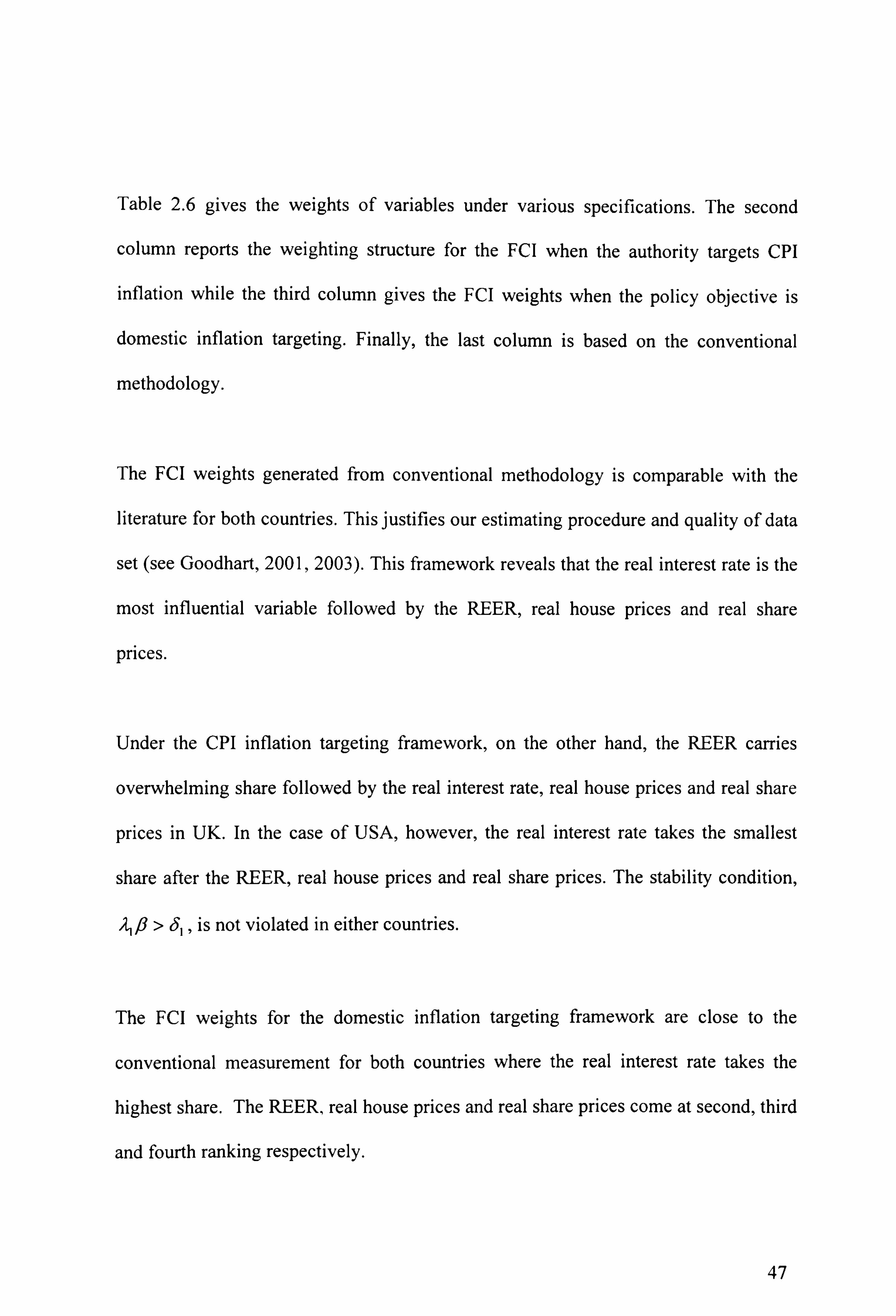
Table 2.6 gives the weights of variables under various specifications. The second
column reports the weighting structure for the FCl when the authority targets CPI
inflation while the third column gives the FCI weights when the policy objective is
domestic inflation targeting. Finally, the last column is based on the conventional
methodology.
The FCI weights generated from conventional methodology is comparable with the
literature for both countries. This justifies our estimating procedure and quality of data
set (see Goodhart, 2001,2003). This framework reveals that the real interest rate is the
most influential variable followed by the REER, real house prices and real share
prices.
Under the CPI inflation targeting framework, on the other hand, the REER carries
overwhelming share followed by the real interest rate, real house prices and real share
prices in UK. In the case of USA, however, the real interest rate takes the smallest
share after the REER, real house prices and real share prices. The stability condition,
1ýfl >, 5,, is not violated in either countries.
The FCI weights for the domestic inflation targeting framework are close to the
conventional measurement for both countries where the real interest rate takes the
highest share. The REER, real house prices and real share prices come at second, third
and fourth ranking respectively.
47
Page 60
Table 2.6: FCI weights
Variables
CPI inflation
targeting framework
(FCI_I)
Domestic inflation
targeting framework
(FCI_2)
Conventional
measurement (FCI_3)
Panel A: UK
Real interest rate 0.154 0.443 0.673
REER 0.659 0.434 0.139
Real house prices 0.130 0.085 0.130
Real share prices 0.058 1
0.038 0.058
Panel B: USA
Real interest rate 0.108 0.307 0.395
REER 0.348 0.270 0.060
Real house prices 0.306 0.238 0.306
Real share prices 0.238 0.185 0.238
Note: See Table 2.2for the methodology and Table 2.4 and 2.5for the estimated
coefficients.
Although the focus of this chapter is to estimate the FCI, we also compute the MCI
weights for the comparison purpose (Appendix 2.2). Not surprisingly, we get the same
message regarding the relative importance of the real interest rate and the REER in the
conduct of monetary policy for both countries (Appendix 2.3 and 2.4)
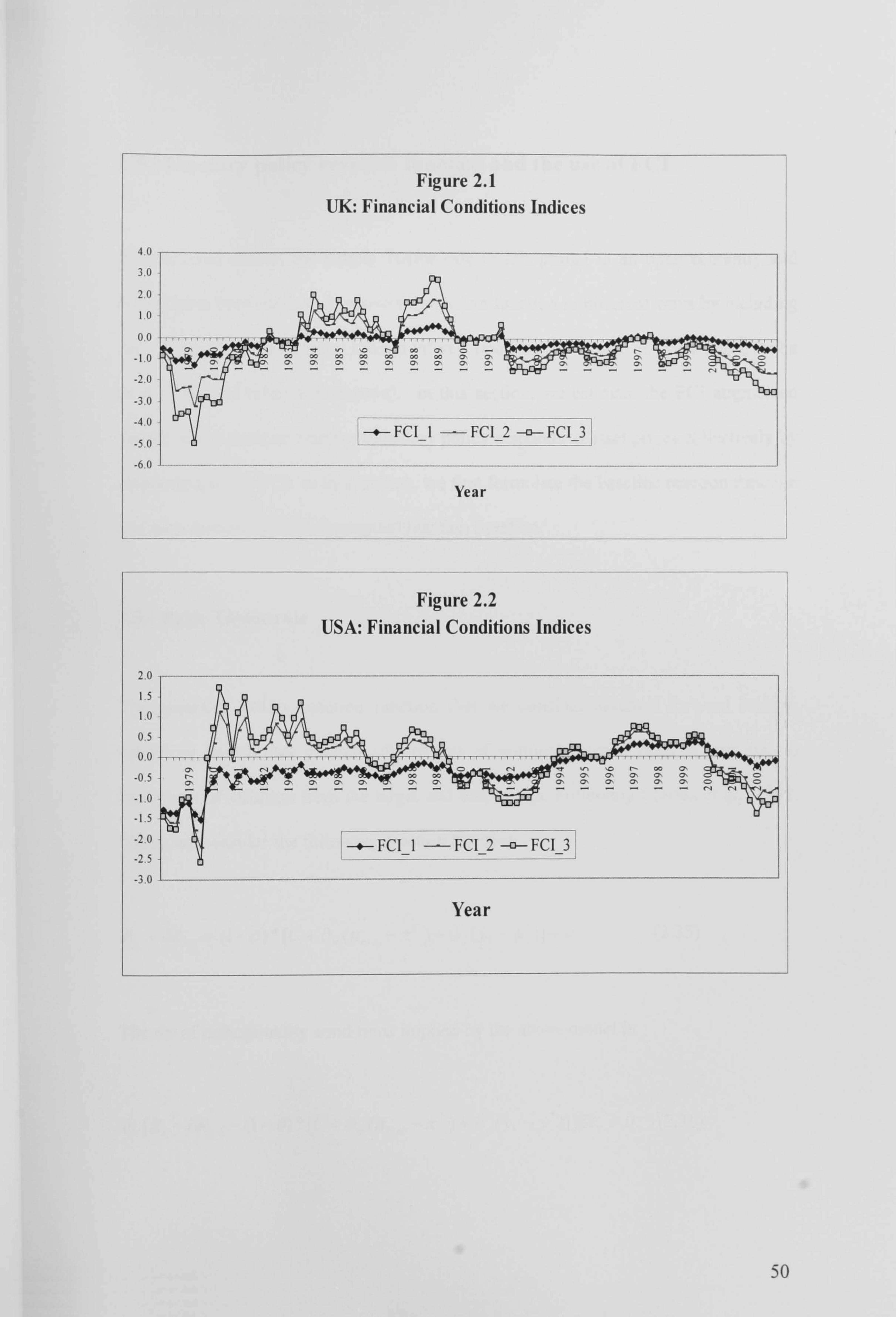
Figure 2.1 and 2.2 plots the FCls for the UK and the USA. The indices are based on
the computed weights as shown in Table 2.6 and historical time series beginning from
48
Page 61
1979QI to 2003Q4. The reference period is assumed to be 2000QI for all
specifications and countries. We emerge the following conclusions from these figures.
First, the UK and USA tightened monetary policy during the 1980s as we find that
both FCI-2 and FIC-3 exceeded the par level. One of the reasons for tightening
monetary policy could be the response to a high level of inflation resulted from the oil
price shocks and relatively a higher level of budget deficits during this period. Not
surprisingly, the FCI-I, however, shows a contradict result for this period which is
less likely to be justified. It is because, as discussed earlier, the FCI-I does not
provide a realistic policy stance when the foreign shocks have a greater impact on
Philips curve. This has been a case for the USA during 1980s (Goldman Sachs, 1999).
Second, policy may have responded to the Asian financial crises in 1997 as the FCl
exceeded the par level. Third, monetary policy has been more accommodative since
the beginning of this century as all indices are below the par level. Fourth, FCIs and
MCls are stable for the ongoing inflation targeting period (post Oct 1992) in UK and
the Greenspan period in the USA, implies that monetary policy has been successftil to
stabilize the inflation.
49
Page 62
Figure 2.1 UK: Financial Conditions Indices
40
3.0
20
l'O
0,0
-1.0
-2.0
-3.0
-4.0
-5.0
-6.0
Year
Figure 2.2 USA: Financial Conditions Indices
2.0
ý5 ýo
0.5 POO
0.0 ................... 45
.5
-10 FCI-l -FCI-2 -c-FCI-3 -2.5
-3.0 - -----
Year
50
Page 63
2.5 Monetary policy reaction function and the use of FCI
As discussed earlier, the simple Taylor rule is suboptimal in an open economy and
efforts have been made to improve the reaction function in different ways by including
asst prices, exchange rates or foreign interest rates (see Clarida et al., 1998 and Chadha
et al. 2004 and references therein). In this section, we estimate the FCI augmented
Taylor rule to analyse whether monetary policy responds to asset prices collectively by
responding to the FCI. In this context, we first formulate the baseline reaction function
and then discuss the FCI augmented reaction function.
2.5.1 Basic Taylor rule
The monetary policy reaction ftinction that we consider assumes forward looking
behaviour and allows gradual adjustments of nominal interest rates in response to
deviations of inflation from the target and output gap. Following Clarida et al. (1998,
2000), we consider the following reaction ftinction.
T)+a *)] + V, R, = aRl-I + (I - a) * [C + a, (ir,.,, -; r , (Y, - Y, (2.35)
The set of orthogonality conditions implied by the above model is:
E, (R, - aR, -, -0- C9) * IC + az (7rt+n - 7r
T)+a
Y(Y, -Y, *)])Iol=O (2.36)
51
Page 64
Where, R, is the short term nominal interest rate, 7r,,,, is inflation at time t+n, 7r T is
targeted level of inflation, y, is actual GDP. y, . is HP trended GDP (calculated by
passing real GDP through the Hodrick Prescott filter with the smoothness parameter
set at 1600). v, is white nose. a, and aY are parameters assigned to inflation and
output respectively. a is the degree of interest rate smoothening and assumed to be
O< a <1 ". Q, is the information set available for policyrnakers while setting R,.
This framework allows a gradual adjustment of the interest rate towards its targeted
level and is found to be superior for the policy purpose for at least two reasons. First,
Goodfriend (1991,1997) argues that the interest rate inertia allows the central bank to
communicate its policy more clearly so that financial instability due arising from
uncertainty could be minimized.
" In the extreme cases, when 13 =0 the Taylor rule does not allow to smooth changes in the interest
rate, indicating that the central bank has a perfect control over short term interest rates. In this case the
model describes a situation that policyrnakers adjust short term interest rates to the desired level as and
when required. The recent literature strongly oppose this case and argues that policy inertia operates in
practice (Clarida et al., 1998, Castelnuovo, 2003, Svensson, 1997 and Orphanides (2002). On the other
extreme when 13 =1 policy does not respond to inflation and output but follows the autoregressive trend
which is again not true in practice.
52
Page 65
Second, Goodhart (1999), Woodford (2001), Orphanides (2001), Judd and Rudebusch
(1998) and Clarida et. al. (1988), among others, find that this type of framework
makes future path of policy change more predictable and helps to increase policy
effectiveness. More specifically, as pointed out by Goodhart (1999), a gradual
adjustment policy framework avoids a frequent policy reversal which is very important
in the conduct of monetary policy because a frequent policy reversal reflects an
incapability of policymakers.
2.5.2 Augmented Taylor rule
Although forward looking monetary policy inertia as discussed above is found to be
superior over conventional Taylor Rule, it has some limitations. First, as pointed out
by Kerr and King (1995), Bemanke and Woodford (1997) and Clarida et al. (1998),
the policy feedback rule itself may be a source of instability if the coefficient of
deviations of inflation from the target (aj is below unity. Second, even if the
coefficient is valid, the policy feedback rule may not capture the market phenomenon
due to the exclusion of other important assets prices like share prices and house prices.
Recent contributions show that share price and assets price help to predict interest rate
more accurately (eg. Montagnoli and Napolitano, 2005).
More specifically, Kristen (2004) argues that the Taylor rule is less important for
policy purpose if financial variables are excluded from the reaction function. He
expands the Taylor rule by including financial market conditions as proxied by
53
Page 66
difference between the short term Treasury bill rate and the long term risky bond and
finds robust estimation for the US (see also Mehra 12 , 1999). Gerlach and Schnabel
(2000) and Clarida et al. (1998) modify the forward looking Taylor rule by including
monetary growth and exchange rate separately and find that these variables contains an
important source in the interest rate setting. They, however, recognized the role of
other assets prices in the feed back rule but do not address them.
Smets (1997), on the other hand, includes the nominal trade-weighed exchange rate, a
ten-year nominal bond yield and a broad stock market index in the augmented Taylor
rule for Canada and Australia but does not give any role to house prices. Goodhart and
Hofmann (2001,2003) find that the FCI contains useftil information in the prediction
of the output and inflation.
In this context, we propose an FCI augmented Taylor rule in which case policy
responds to the FCI as an alternative to each asset prices separately. The augmented
reaction function we consider takes the following form:
R, = c9R, -, + (I
_ a) * [C +az(; 71+1 _, 7
T) +a ,
(Y, - Yl: ) + L9A, iFcIt, i I+ VI (2.37)
and the orthogonality conditions is given by:
12 He use only long term bond rate in his augmented Taylor rule for US.
54
Page 67
E, (R, -aR, -(I-a)* [C +
aT (7rt+,? T+a __O -1 1
(Y' _Y1 _OA, iFC, 1, i
Dlot 7- (2.38)
Where, subscript i (for i=I to 3) indicates three scenarios of FCls as defined in the
previous section and aA,, are corresponding parameters to be estimated.
2.5.3 Estimation procedure
We first estimate the basic Taylor rule as given by Eq. (2.35) and then estimate the
augmented model as given by Eq. (2.37) using Generalised Method of Moments
(GMM) for the UK and the USA. The instruments, 0, are a constant and up to five
lags of the nominal short-term interest rate, inflation, output gap and FCls. Since the
number of instruments are greater than parameters to be estimated, we test for the over
13 identifying restrictions by using Hansen (1982) j-statistics for all estimations . In this
context, the test of the over identifying restriction is very important. A rejection of the
null hypothesis that the over identifying restriction is satisfied implies that instruments
are not orthogonal to the error term. This suggests that the model is mis-specified.
We use quarterly data over the period 1979Q2 to 2003Q4 for UK when controlling
inflation became a clear policy objective and 1979Q3 to 2003Q4 for USA when
Volcker, the then Governor of Fed, signalled his intention to reign in inflation (Clarida
et al., 1998). A full sample estimate is less useful because policy has changed
13 Interpretation of over identifying restriction can be found in Clarida et al. (1998)
55
Page 68
significantly during this period. For instance, UK has adopted inflation targeting since
October 1992. On the other hand, Fed does not target inflation explicitly but it is
argued that it has targeting implicitly in a way of explicit targeting since the beginning
of Greenspan tenure (1987Q3 - 2005Q4). In this context, we split the full sample into
two periods taking 1992Q4 and 1987Q3 as a reference period for the UK and the USA
respectively.
2.5.4 Empirical findings
Table 2.7 reports GMM estimates of the baseline reaction function, Eq. (2.35), for UK.
The Panel A reports estimates for the pre inflation targeting period while Panel B
reports the estimates for the inflation targeting era. Both estimates are quite consistent
with the existing literature as we find policy gives a more weight to inflation and less
to the output gap in the ongoing inflation targeting regime (since 1992) compared to
pre-inflation targeting era (Martin and Milas, 2004).
The estimates of the benchmark model indicate that the nominal interest rate increases
by 1.187 percentage point in response to aI percentage point excess of inflation over
the targeted rate in post 1992 compare to as low as 0.35 percentage point increase in
the previous era. Consequently, the coefficient of output gap found to be as low as
0.50 in the inflation targeting period compare to 1.46 in the pre inflation targeting
period. These results support the exiting empirical literature that the Bank of England
56
Page 69
has been more aggressive to control inflation since late 1992 compared to the previous
era (see also Clarida et al., 1998).
Table 2.7: UK Taylor rule: GMM estimates
[Model: R, = aRt-I + (I - a) * [C + a, (7r f+I - 7r T)+a 1(y, -yl*)+aAFCIII+Vll
Estimated C a, ay aA J-P S. E
Parameters N
Panel A: Pre Inflation Targeting Period (I 979Q2-1992Q3)
Benchmark 0.708 2.584 0.353 1.459 - 0.17 0.99
Model (0.060)* (0.957)* (0.171)* (0.548)* 0.01
Adding: FCI-I 0.593 3.296 0.496 0.838 0.349 0.14 0.85
(0.064)* (0.856)* (0.172)* (0.293)* (0.025)* 0.17
FCI-2 0.628 2.986 0.503 0.849 1.140 0.13 0.86
(0.053)* (0.867)* (0.215)* (0.333)* (0.323)* 0.16
FCI-3 0.639 2.887 0.501 0.867 0.751 0.12 0.86
(0.062)* (0.870)* (0.194)* (0.291)* L
0.277)* 0.15
Panel B: Inflation Týgeting Period (199264-2003Q3 )
Benchmark 0.426 3.559 1.187 0.500 - 0.08 0.63
Model (0.141)* (0.996)* (0.331)* (0.122)* 0.08
Adding: FCI-l 0.398 2.887 1.276 0.435 0.231 0.20 0.49
(0.143)* (0.984)* (0.199)* (0.166)* (0.017)* 0.10
FCI-2 0.386 3.583 1.595 0.564 0.656 0.15 0.61
(0.133)* (0.955)* (0.261)* (0.195)* (0.163)* 0.09
FCI-3 0.399 3.461 1.433 0.584 0.250 0.13 0.63
(0.120)* (1.051)* (0.233)* (0.216)* (0.033)* 0.07
Note:
1. HAC standard errors are employed in the estimates.
57
Page 70
2. Instruments used are a constant, 2 to 5 lags of the dependent variable, and I to 5
lags of inflation, output gap and FCls. The interest rate, deviations of inflation
ftom the target and the output gap are considered to be endogenous variables. 3. Numbers in parentheses are the standard errors of the estimates, N is the
probability value of the normality test, J-P denotes the test statisticsfor over identi ed restrictions. ff,
4. Figures in parenthesis are standard error and *, ** and *** indicate level of
significance at I Yo, 5% and 10% respectively.
We, next, estimate augmented models (Eq. 2.37) by including FCI_I, FCI-2 and
FCl-3 alternatively for UK. As reported in Table 2.7, we find a positive sign of the
FCI coefficients for all specifications. The estimated FCI parameters ranged from 0.23
to 1.14 and are found to be significant at I%. It implies that monetary policy in UK
responds to asset prices collectively by responding to the FCI. Interestingly, the policy
response to inflation is found to be stronger when the FCI is included in the reaction
function, indicating that any deviation in financial conditions from ftindamental may
also create a threat to inflation. We also find that that the interest rate is more
responsive to asset prices (i. e. the FCI) if the policy targets domestic inflation.
We, then, estimate the benchmark model for the USA. As shown in Table 2.8, the
Panel A reports the estimates for Greenspan period while Panel B provides a full
sample estimate. Interestingly, we find that the Fed has been more aggressive to
control inflation during the Greenspan period as we find that the coefficient of
deviations of inflation from the target is higher than the coefficient of the output gap.
However, a weak evidence of orthogonality is alarmed in the benchmark estimate.
58
Page 71
Table 2.8: US Taylor rule: GMM estimates
[Model: R, = aRI-I + (I - a) * [C + a, (7r, +, - 7r
T)+a ,
(y, - yl*) + aAFCI, ]+v, I
Estimated Parameters a C ay aA J-P S. E
N
Panel A: Greenspan period (1987. Q3-2003Q4)
Benchmark 0.847 1.196 2.806 1.466 - 0.06 0.98
Model (0.134)* (0.497)* (0.551)* (0.521)* 0.53
Adding: FCl-l 0.793 1.368 2.165 1.268 0.770 0.39 0.50
(0.046)* (0.327)* (0.781)* (0.482)* (0.256)* 0.23
FCI-2 0.746 2.087 2.574 1.035 0.763 0.38 0.51
(0.055)* (0.421)* (0.92 1)* (0.425)* (0.212)* 0.24
FCI-3 0.730 2.187 2.489 0.914 0.650 0.36 0.48
(0.064)* (0.320)* (0.911)* (0.335)* (0.184)* 0.19
Panel B: Greenspan d Volcker period (1979Q3-2003Q4)
Benchmark 0.918 1.290 2.056 2.063 - 0.07 1.12
Model (0.122)* (0.452)* (0.381)* (0.862)* 0.13
Adding: FCl-l 0.913 1.819 2.206 1.495 0.546 0.27 0.73
(0.224)* (0.462)* (0.425)* (0.490)* (0.102)* 0.17
FCI-2 0.896 1.983 2.278 1.327 0.622 0.26 0.82
(0.110)* (0.335)* (0.491)* (0.282)* (0.242)* 0.11
FCl-3 0.880 1.632 2.848 1.601 0.861 0.29 0.81
(0.123)* (0.343)* (0.691)* (0.582)* (0.324)* 0.12
Note: refer Table 2.7forfootnotes.
59
Page 72
The problem of misspecification could be solved using the second order partial
adjustment reaction function as given by Clarida et al. (1998) or using nonlinear
specifications (see Dolado et al., 2002). But we argue that the misspecification in the
benchmark specification is due to the omitted variable as our FCI augmented reaction
functions are robust. This implies that the FCI contains important information to
predict interest rate. The effect of the FCI is even higher in US than the UK as the
estimated parameter ranged from 0.16 to 0.92 in US compared to a range of 0.26 to
0.42 in UK.
An effort was made to estimate the reaction function using up to 4 th lags of FCIs but
found similar estimates. Similarly, we also tested forward, backward and
contemporariness specifications of inflation and the output gap but the for-ward
looking specifications as given by Eq. (2.35) and (2.37) outperformed to other
specifications.
To sum up, our empirical evidence from the UK and the US reveals that FCI
augmented reaction ftinctions outperform the benchmark model in a number of ways.
First, the standard error is sharply reduced in all augmented models compared to the
benchmark estimate. Second, weak evidence of normality is detected in the benchmark
model for the US but there was no sign of misspecification in the FCI augmented
model. Third, we support the findings of Kristen (2004) that a high degree of
smoothing parameter is due to unobserved variable. It is because smoothing
60
Page 73
coefficient is decreases sharply in our FCI augmented reaction function compared to
the benchmark estimate 14
2.6 Concluding remarks
A large bulk of literature argues that monetary policy should respond to asset prices as
these variables contain important information for predicting inflation and the output
gap (Goodhart, 2001). Although the issue of how and to what extent should monetary
policy respond to asset prices is debatable, there is an argument that policy may
respond to them collectively by responding to the FCI (Goodhart and Hofmann, 2001).
In this chapter, we address this issue extensively on both theoretical and empirical
grounds. By contrast of using the IS curve alone in the conventional literature, we
employ a macroeconomic structural model, which combines both the demand and
supply side of the economy, to obtain the FCI. We explore two alternative FCl models,
one for CPI inflation and another for domestic inflation targeting frameworks
respectively. Although both of them are obtained from a macroeconomic structural
model, the main difference between them is the treatment of the real exchange rate.
14 There is a debate whether a high degree of smoothing parameter is policy inertia or the effect of
unobserved variable. Rudebusch (2002) argues that smoothing can arise spuriously if variables are
excluded incorrectly. Kristen (1999) finds that policy inertia with a high degree of smoothing is less
important for the policy purpose. He suggests that smoothing coefficient could be reduced by the
inclusion of financial variable in the reaction function.
61
Page 74
The CPI model assumes that the real exchange rate has a direct impact on inflation via
import prices and indirect effects via pressure on the aggregate demand while the latter
case considers the indirect impact alone.
On the empirical side, we construct FCls for the UK and the USA using our new as
well as conventional methodologies. We, then, test the usefulness of indices by
estimating the FCI augmented Taylor rule. The empirical results overwhelmingly
suggest that the FCI contains important information in the conduct of monetary policy.
Moreover, monetary authority can respond to asset prices by responding to the FCI as
we find that the FCI augmented Taylor rules outperform the simple rule in both
countries irrespective to the type of FCls and sub-sample periods.
62
Page 75
Chapter 3
Modelling UK Monetary Policy:
A Nonlinear Perspective"
3.1 Introduction
Although a growing number of central banks around the globe have started inflation
targeting since the early 1990s and the short-term nominal interest rate was
considered to be the only effective instrument, the analytical framework of monetary
policy was largely unclear until the seminal work of John Taylor (Taylor, 1993). He
explored a simple linear monetary policy reaction function, in which policyrnakers set
the interest rate in response to deviations of inflation from the target and the output
gap.
15 1 am grateftil to Professor Costas Milas, Keele University, UK, for his helpful comments on the earlier version of this chapter.
63
Page 76
More recent work has extended the Taylor rule. The work can be classified into three
broad groups. First, Clarida et al. (1998,2000), among others, explore a 'smoothing
reaction function' which allows a gradual adjustment in the interest rate towards
equilibrium, an alternative to the 'immediate reactive' type of reaction function. This
framework of monetary policy is assumed to be more transparent and predictable than
the conventional Taylor rule (See also Goodfriend, 1991; Woodford, 2001;
Orphanides, 1998, Judd and Rudebusch, 1998).
Second, Gerlach (2004), Mehra (1999), Clarida et al. (1998), Smets (1997), Chadha et
A (2004), among others, argue that policyrnakers not only respond to deviations of
inflation from the target and the output gap but also to the foreign interest rates and
the real exchange rate. Moreover, Goodhart and Hofmann (2000) and Goodhart
(2001) argue that policy responds to property and equity prices together with inflation
and the output gap.
Third, a number of recent studies argue that the monetary policy is nonlinear and the
policy response is asymmetric. This is due to either a nonlinear loss function (Clark et
al., 1997 and Mayes and Viren, 2001) and/or the existence of nonlinearities in the
economic structure (see Schaling, 1999, Dolado et al., 2000,2003,2004, Stiglitz,
1997, Martin and Milas 2004).
64
Page 77
In this backdrop, this chapter models the UK monetary policy for the post-1992
period, the explicit inflation-targeting regime. The motivation of this chapter is two-
fold. First, although a number of recent studies have argued that UK monetary policy
is nonlinear, this conclusion is based on a narrow framework, the Taylor rule, which
does not account for asset prices or open economy effects. We argue that detection of
the nonlinearity may be due to misspecification of the Taylor rule. Second, expanded
reaction functions have also been explored in the literature but they do not attempt to
analyze nonlinear and asymmetric aspects of monetary policy (for instance see
Gerlach, 2004; Clarida et al., 1998; and Smets, 1997).
This chapter combines these two aspects of the literature. We use asset prices in an
augmented Taylor rule as a benchmark linear model and then use various nonlinear
models including smooth transition autoregressive (STAR) model to estimate reaction
functions (van Dijk et al., 2002 and Martin and Milas, 2004).
Our main findings are as follows. First, the Bank of England responds to deviations of
inflation from the target and the output gap as well as asset prices misalignments, as
we find that the asset price augmented Taylor rule outperforms the simple rule.
Among various asset prices under consideration, however, the policy response to the
exchange rate misalignment is more prominent.
Second, we find that the aim of monetary policy is to keep inflation within a narrow
range rather than pursuing a point target of 2.5% in practice. Policy only responded to
65
Page 78
inflation when expected inflation is in the outer regime. This implies that monetary
policy is nonlinear and the policy response is asymmetric.
Third, the policy response to the output gap and the exchange rate misalignment is
more acute when economy is in the inner inflation regime compared to a response to
them when the economy is in the outer inflation regime.
The rest of this chapter is organized as follows. The next section discusses the
contemporary literature and identifies the research gap. Section 3.3 presents the
methodology followed by empirical findings in Section 3.4. Finally, section 3.5
concludes the chapter.
3.2 Evolution of monetary policy reaction function
John Taylor advanced the following monetary policy reaction function based on US
quarterly data for the period of 1984. Ql to 1992. Q3. Under this rule, short term
interest rates are set in response to the deviation of inflation from the targeted rate and
the output gap (Taylor, 1993).
il = +; T + a, (ir, - )r T)+a
yy, (3.0)
66
Page 79
where, i, is the Federal funds rate, ; r, is the annualized quarterly inflation rate, ; T' is
the targeted rate of inflation, y, is the output gap defined as (Y-Y*) I Y* *100, where
Y is the real GDP and Y* is the potential GDP. In his original model, the average
Federal fund rate, r, and the long run inflation rate, ir, are set at 2 percent each to
meet the steady state economic growth of 2.2 percent. The targeted rate of inflation,
7r', is assumed to be the sample average, i. e. 2 percent, and the feedback parameters,
a,, and t9y . set at 0.5 each.
The underlying model has three basic assumptions: first, the central bank uses short-
term interest rates as the policy instrument. Second, the central bank can
systematically use the interest rate to stabilize inflation and output. And lastly, the
interest rate responds with fixed weights to the deviation of inflation from the target
and the output gap (see also Taylor, 1999a and 1999b).
Although it is widely accepted that the Taylor rule captures the basic characteristics of
monetary policy, at least for the inflation targeting countries, the scope of the use of
the conventional rule is limited in practice for two reasons. First, monetary policy
might be nonlinear and policy response could be asymmetric. Secondly, policy may
not always respond to inflation and the output gap but also to other variables. The
recent contributions, therefore, have addressed these two issues extensively which can
be categorized under the linear and nonlinear monetary policy reaction functions as
follows.
67
Page 80
3.2.1 Linear reaction function
The experiment and extension of the conventional rule under the linear framework
may be summarized as follows:
First, although the conventional Taylor rule provides a contemporary relationship
among the short term interest rates inflation and the output gap, recent empirical
studies suggest that either a backward looking or forward looking specifications better
explains the behavior of monetary policy. Ball (1999), Svensson (1999), Rudebusch
and Svensson (1999) are examples of backward looking models while Clarida et al.
(1999), Domenech et al (2001) and Mehra (1999), among others, favor a forward
looking policy reaction function. The literature, however, presents a consistent result
that monetary policy across countries has been more responsive to inflation than any
other policy variables since early 1990s.
Second, efforts have been made to simulate the liner policy rule using different time
horizons and various structural macroeconomic models. Overall, the results show that
the Taylor rule stabilizes inflation and output in a way close to optimal policy rules in
many macroeconomic models (Ball 1999, Taylor, 1999a and Lansing and Trehan,
2001).
68
Page 81
Third, as the conventional Taylor rule has been expanded by including asset prices
and open economy variables like the foreign interest rates and the exchange rate. For
instance, Gerlach (2004) expands the Taylor rule by including financial market
conditions, proxied by the spread between the short-term Treasury bill rate and a long
term risky bond for the US (see also Mehra 16 , 1999). Gerlach and Schnabel (2000)
and Clarida et al. (1998) include monetary growth and the exchange rate (see also
Chadha et al. 2004). Smets (1997) uses the nominal trade-weighed exchange rate, a
ten-year nominal bond yield and the stock market index in the Taylor rule for Canada
and Australia. Adam et al. (2004), on the other hand, include foreign interest rates in a
Taylor rule estimated for the UK.
Fourth, a survey of empirical studies show that policyrnakers give more weight to
inflation than to the output gap in the inflation targeting regime compared to the
previous era (see Domenech et. al, 200 1, and Gerlach and Schnabel, 2000 for the Euro
area; Nelson, 2000 and Martin and Milas, 2004 for UK and Judd and Rudebusch,
1998, Perez, 2001 and Orphanides, 2001 for the US).
Fifth, the literature argues that the smoothing Taylor rule, which considers a gradual
adjustment of interest rates towards equilibrium, is more appropriate than the
'immediate reactive' policy rule, which does not consider the lag dependent in the
reaction function, for the following reasons. Firstly, interest rate inertia allows the
central bank to communicate its policy more clearly so that financial instability due
16 He includes the long-term bond rate in the reaction function for the US.
69
Page 82
arising from uncertainty in the monetary policy is minimized (see also Goodfriend
1987,1991). Secondly, as discussed in Woodford (2001) and Clarida et al. (1998), a
smoothing reaction function makes the future path of interest rates more predictable.
Thirdly, it is argued that uncertainty about the future state of the economy might
encourage the central bank to change short-term interest rates gradually (see
Orphanides, 1998, Judd and Rudebusch 1998). Finally, it is also argued that interest
rate smoothing enable policyrnakers to avoid frequent policy reversals. This would
make policy more credible as frequent policy reversals may jeopardize the financial
stability (Goodhart, 1999). Therefore, interest rate smoothing is also viewed as an
attempt by policyrnakers to safeguard their reputation (see also Kontonikas, 2004).
3.2.2 Nonlinear reaction functions
Although linear Taylor-type reaction functions give a basic framework for monetary
policy analysis, they potentially neglect asymmetries and nonlinearities that may be
important in practice. As discussed in Clark et al. (1997), if the economy itself is
asymmetric then policy should also have an offsetting asymmetry. Mayes and Viren
(2001) further argue that as long as the hypothesis of asymmetry cannot be
convincingly rejected, policy should assume asymmetry because the cost of wrongly
assuming symmetry when the economy is asymmetric are greater than from assuming
it is asymmetric when actual policy is symmetric.
70
Page 83
The literature finds at least two sources of nonlinearity in monetary policy. First, it is
often argued that policyrnaker's preferences are asymmetric as they have to face a
nonlinear loss function instead of the linear quadratic. This implies that the
policyrnakers show different temptation for controlling positive and negative
deviations of inflation from the target (see Gerlach 2000, Cukierman, 2000, Nobay
and Peel, 1998, and Dolado et al. 2004 among others).
Secondly, it has been recognized that either the supply (Philips) and/or demand (IS)
curve may be nonlinear which implies economic policy follows a nonlinear path. For
instance Schaling (1999), and Dolado et al. (2003) argue that the Philips curve is
convex to the origin. On the other hand, Stiglitz (1997) is in favor of concave Philips
curve.
Huang et al. (2001), on the other hand, argue that the nonlinearity arises from
uncertainty in the productivity. They find that an optimal updating rule for the
NAIRU leads to nonlinear interest-rate policy in Finland. This implies that
policyrnakers are more cautious about adjusting interest rates in response to a small
output gaps than in a standard linear Taylor rule but more aggressive when they reach
a certain threshold.
In this context, Orphanides and Wieland (2000) develop an optimal monetary policy
reaction function based on nonlinear preferences. Ruge-Murcia (2002), Surico (2002)
and Cukien-nan and Muscatelli (2002) also follow the same tradition, assuming
71
Page 84
asymmetric preferences with respect to inflation and/or the output gap. Employing an
asymmetric loss function, Cukierman and Gerlach (2003) show that even if
policyrnakers target the natural level of employment, there will be an inflation bias if
the central bank is more sensitive to policy failures that drive employment below the
normal level than to policy failures that raise employment above it. This suggests that
policy measure is clearly nonlinear.
Nobay and Peel (1998) assume that the central bank has an asymmetric loss function
with regards to both inflation and the output gap. They argue that the asymmetric loss
in inflation results in an inflation bias, which can take either sign whilst the
asymmetric preferences over output gap implies that reducing the target level of
output to the natural rate does not eliminate the inflationary bias.
Dolado et al. (2003,2004) derive optimal monetary policy rules accounting for
uncertainty on the output gap. Using US quarterly data, they find that both sign and
size asymmetries of uncertainty matter in the conduct of monetary policy. Gerlach
(2002) includes the output gap volatility to the Taylor rule and finds that responding
more strongly to recessions than to expansions creates an inflation bias. Moreover, he
argues that output volatility keeps a positive relation to both inflation and recessions,
implying a higher volatility invites a higher rate of inflation and recessions.
Bec et al. (2002) extended theoretical models proposed by Svensson (1997) and
Clarida et al. (1998,2000) by including positive and negative deviations of output
72
Page 85
from trend. They find that changes in short term interest rates are influenced by the
state of the current and or expected state of the business cycle in the US, Germany
and France.
Martin and Milas (2004) use a quadratic logistic smooth transition autoregressive
(QL-STAR) model to analyze the nonlinearity and asymmetric behavior of UK
monetary policy. Using quarterly data from 1972QI-2000QI, they argue that
monetary policy is more responsive to inflation and correspondingly less to the output
gap in the inflation targeting period as compared to the previous era. The response of
policy to inflation is nonlinear as interest rates respond more to positive deviations of
inflation form the target compare to negative deviations. Furthermore, they argue that
the BoE has attempting to keep inflation within a range rather than pursuing a point
target of 2.5%.
In conclusion, nonlinear monetary policy rules have been popular in recent years, not
only because data supports the nonlinear framework but also because the behavior of
policyrnakers itself is nonlinear. In this context Meyer (2000) 17 says:
17 Remarks by Governor Laurence H. Meyer on "Structural Change and Monetary Policy" at a Joint
Conference of the Federal Reserve Bank of San Francisco and the Stanford Institute for Economic
Policy Research, Federal Reserve Bank of San Francisco, San Francisco, California, March 3,2000.
The speech can be found at http: //www. federalreserve. gov/boarddocs/speeches/2000/20000303. htm
73
Page 86
I believe that a nonlinear rule may dominate a linear
specification..... such a nonlinear rule could be justified either by
nonlinearities in the economy or by a non-normal distribution of
policyrnakers' prior beliefs about the NAIRU. It is certainly easy to
believe that there are nonlinearities in the economy in general and with
respect to the Phillips curve in particular... "
3.3 Methodology
3.3.1 General strategy and modelling framework
This chapter models the UK monetary policy for the ongoing explicit inflation
targeting regime, post- 1992. Therefore, the analytical framework we consider in this
chapter assumes that the aim of monetary policy is to target inflation using short-term
interest rates as the main operating instrument. Moreover, the central bank is assumed
to be autonomous, at least at the operational level, so it can set monetary instruments
freely in order to achieve the objective.
We begin our analysis by estimating a simple linear reaction function that combines
the interest rate, deviations of inflation from the target and the output gap. We, then,
augment the ftinction by including a set of financial variables such as real exchange
rate, house prices, and share prices.
74
Page 87
Using an augmented Taylor rule as a benchmark linear specification, we then estimate
nonlinear reaction function using various nonlinear econometric models. We begin
with the Escribano and Granger (1998), Escribano and Aparicio (1999) and Granger
and Lee (1989) models to test whether there is any sign and/or size asymmetries of
deviations of inflation from the target. Although these models provide an indication of
nonlinearity, they are too simple to describe distinct regimes for inflation. Therefore,
in order to analyze nonlinear and asymmetric policy behavior together, we employ the
Smooth Transition Autoregressive (STAR) family of models 18 .
3.3.2 Benchmark specification
3.3. Z 1. Taylor rule
To begin with, we assume that the central bank sets the short-term interest rate in
response to the future deviation of inflation from the target and the output gap, albeit
gradually. Following Clarida et al., (1998,2000) the monetary policy reaction
function that we consider is:
it = bit-, + (I - b)i (3.1)
(3.2) i, =)6+bE, -1(7r,,,, -7r*)+byEt-I (Yt+n - Yt+n)
's Chapter 5 describes the model in detail.
75
Page 88
Where, i, is the observed nominal interest rate, i is the desired interest rate, 8 is
the equilibrium interest rate, E, _1
is the expectation formed at t given the information
of t-1,7r, +, is the expected inflation at time t+n, 7r* is the targeted rate of inflation,
Yt+n is actual GDP at time t+n, y, *+, is the potential GDP at time t+n, and v, is white
nose error term. b, and by are parameters to be estimated.
Eq. (3.1) is the first order partial adjustment function where the observed interest rate,
ij , is defined as a weighted average of the previous period rate and the desired interest
rate. We employ the first order partial adjustment model but it can be extended up to
n th order depending on the nature of data. For instance, Clarida et al. (198 8) employ a
second order partial adjustment model for the US reaction function while they use the
first order partial adjustment model for the European countries including UK.
Combining Eq. (3.1) and (3.2), we obtain
i+ bi il-I + (I - b, ) [b,, Et-I 7r + by El-I (Yt+n - Yt+n A +'61 (3.3)
76
Page 89
where =(I - b, ), 8 is the equilibrium interest rate, b, is the degree of interest rate
smoothening and assumed to be O< b, <1 19 and c, is a stochastic error term which
combines the forecast errors of inflation and output and the random error, vt.
3.3.2.2. Augmented Taylor rule
Although, Eq. (3.3) is considered to be an improvement over the conventional Taylor
rule, it has also some limitations. First, as pointed out by Kerr and King (1995),
Bernanke and Woodford (1997) and Clarida et al. (1998), the policy rule may be a
source of instability if b, is below unity. Second, the policy rule may not work well
in practice if relevant variables are omitted from the reaction functions. This implies
that the Eq. (3.3) may be mis-specified.
In the context of UK, a number of variables like the real exchange rate, the real house
prices and the real share prices have been considered to be relevant in the conduct of
19 When b, =1, the Taylor rule collapses, implies that policyrnakers do not respond to inflation and the
output gap. In the other extreme when b, =0, the resulting function becomes a forward looking Taylor
rule without lag dependent. In this case, the reaction function does not allow us to smooth changes in
interest rate, indicating that the central bank has a perfect control over the short tenn interest rate. It
also implies that the interest rate can be adjusted immediately to its target level as and when required.
This situation, however, is less likely to happen in practice (see Clarida et al. 1998, and 2000,
Castelnuovo, 2003, Svensson, 1997, Orphanides, 2002 among others for the detailed analysis).
77
Page 90
monetary policy 20 (Goodhart and Hofmann 2001,2003; Batini and Tumbull, 2000).
We, therefore, include all these asset prices in the linear specification but select only
the real exchange rate (RER) augmented Taylor rule for the nonlinear specifications
for two reasons. First, the preliminary experiments suggest that the policy response to
RER misalignment is higher than to any other asset prices 21 . Second, our sample size
is not big enough to include all possible asset prices in nonlinear models.
Therefore, we consider the following augmented Taylor rule as a benchmark model
for nonlinear estimates:
i +bji, Y: -1 + (I - bj) * [b,, E, -,
(ir, +,, - ir + byEt-I (Yt+n 1+
beE, -,
(e, - e, *)] + c, (3.4)
where e, is the real effective exchange rate, e* is the equilibrium real exchange rate as
approximated by the HP filter method. b, is the feedback parameter of e, - e* and is
expected to be positive because an increase in e, indicates the depreciation of national
currency vis-d-vis foreign currencies.
20 The previous chapter provides evidence about this.
1 The next section provides empirical evidence on this
78
Page 91
Notice that c, is a linear combination of forecast errors of deviations of inflation from
the target, the output gap and the exogenous disturbances. Therefore, it has to be
orthogonal to variables included in the information set (say, Q, ). A failure to reject
orthogonality implies that lagged variables enter in the reaction function only to the
extent that they forecast future inflation or output (Clarida et al., 1998 and 2000 and
Chadha et al., 2004). Formally, the orthogonality condition can be written as
fil -i- bi il-I - (I - b, ) lb,, (; r,,,, - 7r + by (Yt+n - yt * +,, + b, (e, - e, )))IQ, 0 (3.5)
Eq. (3.5) is the orthogonality condition implied by Eq. (3.4) where Q, is the vector of
all variables that are taken into consideration by the central bank when taking the
monetary policy decision.
3.3.3 Nonlinear modelling
3.3.3.1. Size and sign asymmetries
After estimating the linear benchmark reaction function, that is Eq. (3.4), we then
proceed to analyze various aspects of nonlinearities in the reaction function that are
generated from deviations of inflation from the target, ; T,,, -; r* -
79
Page 92
We first use the Granger and Lee (1989) model to test for sign asymmetries. This
model includes positive and negative deviations of inflation from the target separately
(Dolado et al., 2000), it can be written as:
it =a+ bil-I + (I - b, )[b,,, (; r, +,, - 7r*)+ + b,,,, (7r,.,,, - 7r*)- + by (Yt+n - Yl"+n)
b, (e, - e, + u, (3.6)
Where, - 7r *)'=-
7r *) if -; 7*) ý! 0 and is zero otherwise,
(7rt+n -; r*)- =(7rt+n -7r*) if (; rl+n -ir*)<0 and is zero otherwise. b; r, p and b,,,, are
the key parameters in this model. We test the null hypothesis HO : b,,, p = b,,,, against
H, : b,, P : P, - b,,,,, to identify the sign asymmetry. Rejecting the null implies that
policyrnakers respond to positive and the negative deviations of inflation from the
target differently. This model, however, simplifies to the linear model in Eq. (3.4) if
we do not reject the null hypothesis.
We then estimate the Escribano and Granger (1998) and Escribano and Aparicio
(1999) model to test whether there is any size effects of 7r, -,,, -; r* in the conduct of
monetary policy. This type of model recently used by Arghyrou et al. (2005) to
analyze inflationary dynamics for UK, Martin and Milas (2004) to examine monetary
policy reaction function for UK; and Dolado et al. (2000) to test the output gap
80
Page 93
asymmetry for the US monetary policy reaction function. The model can be written
as:
il =+b, il-I + (I - b, )[b,,, - 7r*) + b,, 2
GTI+n _ ý71)2
yl*+, ) + be (e, - e, *)] + u, (3.7)
Eq. (3.7) compares to (3.4) except for the term b, 2 (7rt+n
_ Ir* )2 where,
bir, 2 measures
the size asymmetry of deviations of inflation from the target. In this model, we test a
null hypothesis, HO : b,,, 2= 0 against the alternative H, : b,, 2 ;, - 0. Rejecting the null
implies that policy responds differently for large and small deviations of inflation
from the target, i. e. the size matters in the interest rate setting. The model simplifies to
the linear benchmark reaction function in Eq. (3.4) if we do not reject the null
hypothesis.
3.3.3.2. Smooth transition autoregressive models
The sign and size hypotheses as given by Eq. (3.6) and (3.7) are simple extensions of
the linear reaction function. One of the limitations of them is that they do not describe
the adjustment process even when the sign or the size of deviations of inflation from
the target matters. Therefore, we next employ smooth transition autoregressive
(STAR) family models to analyze whether monetary policy is nonlinear and policy
81
Page 94
response is asymmetric. This class of nonlinear models is flexible in nature and
provides a number of alternative specifications (see Chapter 5 for more discussion).
As discussed in Granger and Terasvirta (1993), Terasvirta and Anderson (1992) and
Terasvirta (1994), there are three steps to be followed to arrive at the final estimable
STAR model. The first step is to test linearity. If it is not rejected then nonlinear
model, especially STAR models, does not provide any better result over linear ones.
Therefore, we only estimate the nonlinear reaction function using STAR models if
linearity is rejected. The second step is to select a transition variable. This variable is
the sources of nonlinearity in the model as we obtain regimes for this variable. The
third step is to choose an appropriate transition function if there is a lack of economic
theory to be used.
Formal linearity test
As discussed, a formal linearity test is required before employing any nonlinear
models. In this context, we use the testing approach proposed by Saikonnen and
Luukkonen (1988), Luukkonen et al. (1988), Granger and Terasvirta (1993),
Terasvirta and Anderson (1992) and Terasvirta (1994). This test is based on the
following artificial regression.
(1)
il =A+ßoo, +2ý[ßl�0, -j(Z, -d -'7*)+ß2, j0, -j('7t-d _7r*)2 + ß3,
i Ot-i (7r(-d _ ý7)3 + 171 (3.8)
]=o
82
Page 95
Where, A is the constant tenn, 0, is a vector of
{'r-lJ'rt+n -7r*), (Y,,,, -y, *+,, ), (e, -e, *) 1,77, is a white nose error term and 8j (for j= I
to k) are parameters to be estimated for different values of the delay parameter, d. The
linearity test implies the testing of null hypothesis, Ho: )61,, =": )62, j ==0 against
alternative that at least one of them is non-zero. This can be done with a standard
Lagrange Multiplier (LM) type test.
Selection of a transition variable 22
As discussed earlier, the purpose of this chapter is to model the UK monetary policy
for the explicit inflation targeting regime. Therefore, the main objective of estimating
nonlinear reaction function using STAR model is to examine whether the size and/or
sign of deviations of inflation from the target matters for the policy purpose and also
to test whether there exists any asymmetric adjustment of this variable. In this light,
we only consider ýT, -d-7r* as transition variable where d is the 'delay parameter'.
We estimate Eq. (3.8) using a series of d such that -n:! ý d :! ý n and report the linearity
test for all values of d (van Dijk et al, 2002). The maximum number of d is set using
the AIC and the partial autocorrelation of ; r, - 7r* (Iregui et al., 2002).
22 We consider the single transition variable in this chapter. The use of multiple transition variables can
be found in Chapter5.
83
Page 96
Finally, the decision rule is to choose the value of d that rejects linearity most
decisively (van Dijk et al., 2002). If the linearity is rejected for more than one value of
d, then we select the one which gives the lowest p-values (see Terasvirta and
Anderson, 1992 for more discussion).
Selection of transition functions
The literature provides mainly two alternative transition functions for the STAR
model. They are the logistic smooth transition function (LSTAR) and the quadratic
logistic smooth transition function (QL-STAR). The former describes the sign
asymmetry while the latter gives a size asymmetry of the transition variable 23 . There
is a fon-nal procedure for selecting one against another but we use both of them to
estimate the nonlinear reaction function, as our sample is relatively small to rely on
the test statistics.
The literature also provides an exponential smooth transition function to describe the size
asymmetry. However, as discussed in Iregui et al. (2002), van Dijk et al. (2002) and Martin and Milas
(2004), the ESTAR model simplifies to the linear model if either )/ -ý 0 or )/ --+ 00 . For this reason,
we do not estimate the nonlinear reaction function using exponential transition ftinction.
84
Page 97
Nonlinear reaction function
In the light of above discussion, we estimate the nonlinear reaction function using
logistic ftinction as given below (van-Dijik et al., 2002 and Martin and Milas, 2004):
Pt-I + (1 - P)IOIMLI + (1 - Ot)MUI + ýt iid(O,
Where,
MLI ,,,: k, I (7r, -; r +k ,)+k 12 (Yt+n - Y: 13(e, -e, )
Mul = k2l 071+n
-; r*) + k22 (Yl+n - Y, *+n)
+ k23 (e, - e, *), and
Ot = Pr{ rý (ZI-d
- 7r *»=1-
(3.9)
I
+ e-' Orl-d - 7r rD1 Sx
>0
Eq. (3.9) is a nonlinear reaction function in which i, is a weighted average of a "lower
regime", "L, and an "upper regime", Mu, where ML, and Mu, are augmented
Taylor rules similar to Eq. (3-4). 0, is the relative weights assigned to ML, and is
bounded between 0 and 1. In this model, 0, is the probability that" ýý 07, -d-; r) and
consequently (I - 0, ) is the probability that "< (7rt-d - 7r * ). Therefore, the model
describes the sign asymmetry of transition function, 'T' I-d
85
Page 98
The transition function, 0, is determined by the combination of the transition variable,
7r i-d - /T and nuisance parameters (r and The first nuisance parameter, r, is
frequently referred to as the 'threshold parameter', while the latter one is the 'slope
parameter'.
The slope parameter, a, which determines the smoothness of the changes of transition
from one regime to another, has important implication in this model. When
u -> 00 , 0, becomes a heaviside ftinction. In this case, 0, ýO if (Tl
-d - 'T
*) :5T
and 0, =l Secondly, when a --> 0 the logistic function becomes
constant and the model simplifies to be the basic linear model in Eq. (3.4). We make
a dimension free by dividing it by the standard deviation, s, , of 7r, (van Dijk et al.,
2002; and Iregui et al., 2002 for more discussion).
The LSTAR model simplifies to the benchmark linear model in Eq. (3.4) if
k1j = k2j (for all j=1 to 3). There is a sign asymmetry in the reaction function if
k1l # k2l *In practice, we expect k, I<
k2l
ý k2l > k22and k2, >
k23 as policyrnakers
give more attention to inflation and less to output gap and RER if > 7r*. This
model, however, does not describe the size asymmetry.
86
Page 99
We next estimate the nonlinear reaction ftinction using the QL-STAR model as an
alternative to the LSTAR model. This model also provides two regimes for inflation
but the main difference between the LSTAR and QLSTAR is that the former provides
the lower and upper regime while the latter gives the inner and outer regime. In the
latter case, we consider the economy is in the inner inflation regime when expected
inflation is close to the target or remains within two inflation boundaries. On the other
hand, the economy remains in the outer inflation regime when expected inflation is
below the lower boundary or exceeds the upper boundary.
The QL-STAR reaction function can be written as:
+ Pit-I +0- P) 10, MI, +0-0, )Mo, I+
Where,
MI, : -- kll(, 7�� -ir*)+kI2(YI+n -y�n)+k]3(e, - e, )
Mol = k2l (7r,.,,,
- 7r *)+ k22 (Yl+n - yl*+n )+ k23(e, - e, ) and
(3.10)
Pr(-r L<(, 7 1-d - 7r* ): 5 -rU )=1-*1L >o
1+ e-' (Ti-d-ff -r )(7ri-d-yr
Eq. (3.10) describes i, as a weighted average of the inner regime, M1, , and outer
L
regime, MO,. There are two thresholds in this model, the lower threshold ) and
the upper threshold ( r" ), which determines two distinct regimes. The model gives the
87
Page 100
inner inflation regime when rL <- 071-d - 7r* ) ý5 'r
U and the outer regime otherwise.
When economy is in the inner regime, the interest rate is determined by MI, *
Similarly, the interest rate is determined by MO, when the economy is in the outer
inflation regime.
In this model, the transition function 0, has two important properties. First, 0,
becomes constant and hence model simplifies to the benchmark model in Eq. (3.4)
when a -). 0. Second, when a --> -o, 0, =0 if (rl -d
- 7r *)
ýý T or (7r, -d - 7r*)> T
and 0, =1 when TL -<(7r, -d r". Following Granger and Tersvirta (1993) and
Terasvirta (1994) we make the slope parameter dimension free by dividing it by the
variance of inflation ( s, )
As in the LSTAR, The QL-STAR function simplifies to the linear benchmark model
in Eq. (3.4) if k1j = k2j (for all j=1 to 3). The size of deviations of inflation from the
target matter if k, 1# k2l Monetary policy is asymmetric if we reject the null
hypothesis HO : [(7r* _ rL )+ (7r* +u )] /2=2.5% against an alternative hypothesis,
H, : [(lr* _. rL)+(lr* + u)] /2#2.5%.
88
Page 101
3.4 Empirical estimates and discussion
3.4.1 The data
We model UK monetary policy for the ongoing inflation targeting regime, that is,
1992Q4 - 2004Q2. We use the three-month Treasury bill rate as the nominal interest
rate, i, and the four-quarter change in the retail price index (RPI) as the inflation
rate, 7r, . Similarly, real GDP is used as output, y, and the trade weighted real
effective exchange rate index (RER) as the exchange rate variable, e, where an
increase indicates depreciation of home currency vis-a-vis foreign currencies. All
data are obtained from the International Monetary Fund provided by DataStream.
Although the official inflation target (7r*) varies over time in UK 24 , we set it to
2.5%, a periodic average, throughout the period to make comparable with other
studies (Martin and Milas, 2004, Clarida et al., 1998, and Nelson, 2000). In order to
obtain the potential output and the equilibrium RER, we use the Hodrick-Prescott
filter. The output gap (y, - y, .) and the deviation of RER from the equilibrium
( e, -e*) are, therefore, defined as the difference between the actual variable and the
corresponding Hodrick-Prescott trend. The plots of variables are given in Figure 3.1,
below.
24 It was set to a range of I% to 4% for October 1992 to April 1997 and 2.5% thereafter (Bernake et al.
1999).
89
Page 102
We employ augmented Dickey-Fuller (1979) and Phillips-Perron (1988) tests to
assess the stationary of the variables. As discussed in the previous chapter, while the
former test makes a parametric correction for higher-order serial correlation by
assuming that the series follows an autoregressive process with order AR(P) and
adjusts the test methodology by adding lags of independent variables, the latter tests
a unit root through a non-parametric correction procedure (Benerjee et al., 1993).
Table 3.1 presents the test results. The order of integration of i, is found to be more
ambiguous but following Clarida et al. (1998), Martin and Milas (2004) and Fuhrer
(1997), among others, we consider this variable as stationary. Other three variables
( 7r, - 7r *, yt - y, * and e, -e*) are found to be stationary at I %.
Moreover, the literature argues that the linear unit root tests (ADF and PP tests) are
less powerful to detect the stationarity if variables take a nonlinear adjustment process
(Gregoriou and Kontonikas, 2006). In this context, the recent theory and the empirical
literature related to the purchasing power parity, real exchange rates and monetary
policy rule (eg. Sarantis, 1999, Chortareas et al. 2002 and Martin and Milas, 2004)
suggest that inflation and the real exchange rates follow a non-linear mean reverting
process in which case the linear unit root tests may be insufficient to test the
stationarity. Therefore, following Kapetanious et al. (2003), we employ an
exponential smooth transition autoregressive unit root test to evaluate stationarity
90
Page 103
process for 7r, - 7r* and e, - e*. The detail methodology is given in Appendix 2.2.
The empirical estimates firml y suggest that there is no need to doubt about the
sationarity of both variables as we obtain sufficiently a high t-ratio 25 .
Table 3.1: Unit root tests (1992Q4 - 2004Q2)
Variable Description ADF PP Test
Name Test
it 3 Month Treasury Bill Rate -2.58*** -2.19
17t -; r* 4 quarter change in retail price index (RPI) less the -3.77* -2.96** target (2.5%)
1Y -Y* I Output gap -3.99* -3.99*
e, - e, * RER misalignment -7.09* -6.98
Note:
(a) Y, . and e, * are Hodrick- Prescott trends with smoothing parameter set at 1600.
(b) Critical values for the ADF and PP-Test are -3.5 7, -2.92 and -2.60 at 1%, 5%
and 10% significance level respectively.
The superscripts t ** and *** in column (iii) and column (iv) indicate
significant at 1%, 5% and 10% respectively.
25 The computed t-ratio for the coefficients of the cubic ; T, - 7r * and e, -e* are 5.98 and 7.87
respectively.
91
Page 104
Figure 3.1: Plots of variables
a. Three-month Treasury bill rate, i, b. RPI Inflation, 7r,
93 94 95 96 97 9B 99 00 01 02 03
c. Output gap, y, - y, * d. RER misalignment, e, - e, *
93 94 95 96 97 98 99 00 01 02 03 93 94 95 96 97 9B 99 00 01 02 03
92
93 94 95 95 97 9B 99 00 01 C2 03
Page 105
3.4.2 Linear estimates
We begin our empirical analysis by estimating Eq. (3.3) by GMM and OLS. We
experiment various time horizons for the explanatory variables ranging from the 4 th
quarter lag to 4 th quarter lead (-4:! ý n :! ý 4 ). Empirical estimates 26 , however, reveal
that the one period ahead forward looking smoothing Taylor rule outperforms other
specification irrespective of the estimation method. Therefore, unless otherwise
stated, we use n=l for inflation and the output gap and n=O for the RER as time
horizon of variables for all reported estimates. This is consistent with many empirical
studies (eg. Clarida et al., 1998, Chadha et al. 2004 and Adam et al. 2005).
Estimates of Taylor rule (Eq. 3.3) are presented in columns (i) and (ii) of Table 3.2
where the Column (i) presents OLS estimates and column (ii) provides GMM
estimate. Consistent with the empirical literature (Martin and Milas, 2004, Clarida et.
al., 1998 and Nelson, 2000) our GMM and OLS estimates satisfy the dynamic
stability criterion since b, is found to be greater than 1, parameters are significant at
I% with expected positive sign and the condition b,, >by is satisfied. Also z, is
found to be highly persistent as b, is close to 0.9. This all implies that the Bank of
England has given more weight on the price stability and correspondingly less weight
on the output stability during the ongoing inflation targeting era.
26 Not all of them are reported to save space but are available on request.
93
Page 106
Table 3.2: Estimates of linear reaction functions (1992Q4-2004Q2)
Variables Estimate of Eq. (3.3) Estimate of Eq. (3.4)
OLS
G)
GMM
(ii)
OLS
(iii)
GMM
(iv)
0.62 (0.220)* 0.83 (0.085)* 0.576 (0.202)* 0.768 (0.109)*
b, 0.87 (0.040)* 0.84 (0.015)* 0.879 (0.036)* 0.841 (0.020)*
b, 2.50 (0.799)* 2.35 (0.223)* 2.233 (0.713)* 1.447 (0.246)*
by 1.76 (0.837)** 1.16 (0.42 1)* 1.606 (0.781)* 1.127 (0.378)*
b, 0.139 (0.058)* 0.124 (0.009) *
-2 R 0.87 0.86 0.89 0.88
s. e. 0.36 0.37 0.34 0.35
LM4 1.38 [0.25] 1.21 [0.32]
ARCH4 1.96 [0.11] 1.26 [0.30]
F-H 1.54 [0.18] 0.63 [0.74]
F-xH 2.01 [0.06] 0.54 [0.88]
Normality 2.04 [0.351 1.85 [0.39] 1.03 [0.59] 0.38 [0.42]
J-P statistics 0.18 0.20
p-value 0.89 0.92
Notes:
a. Figures in parenthesis are standard error. t ** and *** indicate level of
significance at 1%, 5% and 10% respectively. Numbers in square brackets are p
value of the test statistics. The interest rate, deviations of inflationftom the target
and the output gap are considered to be endogenous variables.
b. s. e. is the standard error of the regression. LM4 is the fourth order Breusch-
Godfrey's Lagrange Multiplier F-testfor the residual serial correlation. ARCH4
is the fourth order auto regression conditional heteroscadasticity F-test. F-H is
the White's heteroscadasticity F-test of residual while F-xH is the test of cross
heteroscadasticity. Finally, RESET is specification error test of the regression
94
Page 107
due to Ramsey (1969). P-value is the probability that the over identified
restriction is satisfied under null.
c. As in Clarida et aL (1998) instruments used for GMM estimates are a constant
and up to five lags of all variables used in the reaction function.
Our GMM estimate is robust as we do not reject the null hypothesis that the
overidentifying restriction is satisfied. The OLS estimates has heteroscadasticity
effects, albeit, marginally.
We next estimate the RER augmented Taylor rule as given by Eq. (3.4). The estimates
are presented in columns (iii) and (iv) of Table 3.2. We estimate b, =0.12 by GMM in
Column (iv) and 0.14 by OLS in Column (iii), both are significant at I%, both imply
that policyrnakers not only respond to deviations of inflation from the target and the
output gap but also to deviations of RER misalignment. Also, these estimates do not
alter the main findings of the simple Taylor rule as discussed earlier.
The augmented Taylor rule outperforms the simple rule for two reasons. First,
standard error has improved significantly in the augmented model. Second, there is no
misspecification in the estimates. Therefore, a RER misalignment augmented Taylor
rule is our preferred estimate over the simple Taylor rule.
As discussed in the previous chapter, share prices and house prices are also
considered to be important variables for UK monetary policy. Therefore, we estimate
95
Page 108
Eq. (3.4) by including deviations of house price from the trend ( h, - h, .) and
deviations of share prices from the trend (s, - s, .) as an alternative specification to Eq.
(3.3) and (3.4). The specification of more expanded Taylor rule is as follows:
il =+b, il-I + (I - b) * [b, (7r, +, - 7r) + b, (y,
+, - yl*+, ) + b, (e, - e, .)
bh(h, - h, *) + b, (s, - s, *)] + c, (3.4a)
Where, h, 4 and s, * are obtained using the Hodrick-Prescott trend as usua, 27.
Table 3.3 presents the empirical estimates of (3.4a). We observe that deviations of
house prices from the trend, h, - h, ., and deviations of share prices from the
fundamental, s, - s, , significantly and positively enter in the reaction function
without altering the previous findings. The estimates, both by GMM and OLS,
confirm that the response to deviations of inflation from the target is more vigorous
followed by the output gap, RER misalignment, deviation of house prices from the
trend and the deviation of share prices from ftindamentals 28 . This result is consistent
with the previous chapter and ftirther justifies the use of asset prices in the conduct of
monetary policy 29
27 The sources and further definitions of variables are given in Chapter 2.
28 This finding is fairly consistent with Goodhart and Hofmann (2001).
29 The expanded Taylor rule may be considered as an alternative to the FCI augmented Taylor rule as
discussed in the previous chapter. It is because the FCI includes all asset prices that are considered in
the expanded Taylor rule. The FCI augmented Taylor rule was superior over the simple rule in the
96
Page 109
Table 3.3: The estimates of expanded Taylor rule# (1992Q4-2004Q2)
OLS Estimate GMM Estimate
0.444 (0.201)* 0.321 (0.059)*
b, 0.905 (0.036)* 0.908 (0.011)*
b, 2.550 (0.872)* 2.152 (0.305)*
by 1.632 (0.836)* 1.394 (0.180)*
bý 0.132 (0.159)* 0.116 (0.059)*
bh 0.031 (0.012** 0.052 (0.028)**
b, 0.044 (0.020)** 0.059 (0.022)**
Diagnostic tests -2 R 0.88 0.88
s. e. 0.33 0.35
LM4 1.50 [0.21]
ARCH4 1.75 [0.15]
F-H 0.75 [0.68]
Normality 0.15 [0.92] 2.44 [0.29]
J-P 0.19
p-value 0.989
Notes: # Estimate of Eq. 3.4a. See Table 3.2 for the footnotes.
previous chapter while expanded Taylor rule outperformed the simple rule in this chapter, both justified
the role of asset prices in the conduct of monetary policy in UK.
97
Page 110
Despite this fact, we, however, do not include house prices and share prices in the
nonlinear estimates for three reasons. First, the estimate of the extended Taylor rule
does not provide a remarkable improvement over the RER augmented reaction
function as the standard error of the estimate has decreased only marginally. Second,
the response of interest rate to asset prices is almost negligible although the
coefficients are significant. Third, our sample size is relatively small to include all
possible asset prices in a nonlinear reaction function. We, however, address the issues
of asset prices in the following chapters.
3.4.3 Nonlinear estimates
3.4.3.1 Accounting for sign and size asymmetries
The benchmark linear Taylor rule suggests that the deviation of expected inflation
from the target, E, -1(7r,,, -7r*), is the most influential variable followed by the
expected output gap, E, _,
(y, +, - y, +,
), and the RER misalignment (e, - e, ). We now
proceed to analyze whether the sign and/or size of the deviation of inflation from the
target matter in the conduct of monetary policy by estimating Eq. (3.6) and (3.7).
98
Page 111
Table 3A Tests of size and sign effects (OLS Estimates: 1992Q4-2004Q2)
Coefficients Sign effect (Estimate of Eq. 3.6)
Size effect (Estimate of Eq. 3.7)
0.532 (0.180)* 0.565 (0.186)*
b, 0.854 (0.033)* 0.861 (0.034)*
b,,, p
3.847 (0.957)*
b,,,, 0.552 (0.6548)
b,,,, 2.327 (0.586)*
b,,, 2 1.017 (0.488)**
by 2.128 (0.667)* 2.128 (0.415)*
b, 0.113 (0.042)* 0.115 (0.056)*
Diagnostic tests -2 R 0.92 0.92
s. e. 0.27 0.28
LM4 1.79 [0.15] 0.82 [0.53]
ARCH4 1.61 [0.18] 1.46 [0.22]
F-H 1.17 [0.33] 0.82 [0.59]
F-Xh 1.16 [0.35] 0.85 [0.63]
Normality 1.81 [0.40] 0.76 [0.62]
RESET 1.07 [0.30] 1.26 [0.26]
No asymmetry (Ho: b,, p
b,,,,, ) 6.02 [0.00]
No Size effects (HO: b,, 2 ý0) 4.34 [0.04]
Notes: Please refer to Table 3.2for thefootnotes.
99
Page 112
Columns (i) of Table 3.4 presents the estimate of Eq. (3.6). We estimate b,, P = 3.85
and b,,,, =0.55. As b,,, P
is significant at 1% but b,,,, is insignificant, it is obvious
that we reject the null hypothesis HO : b,, P = b,,,, in favor of
alternative H, : b,, P : P, - b,,,, . This suggests that monetary policy is nonlinear and
policy only responds to inflation when expected inflation exceeds the target. The
policy response to the output gap and the RER misalignment is found to be similar
with the linear estimates.
We next estimate the Escribano-Granger (1998) and the Escribano and Aparicio
(1999) model, given by Eq. (3.7), which allows size asymmetries. The estimate of
this model is presented in the last column of Table 3.4. In this case, we estimate
b,, 2 ý 1.02 and reject the null hypothesis that HO : b,, 2=0 against the
altemative H, : b,,, 2 #0 at I%. The estimates of other parameters are also fairly
consistent with the previous estimates.
3.4.3.2 Formal nonlinearity tests
The estimate of Granger and Lee (1989) and Escribano-Granger (1998) models
suggest that monetary policy in UK may be nonlinear but as discussed earlier they do
not provide a decisive level of nonlinearity. We now proceed to test the (non)linearity
formally by estimating Eq. (3.8).
100
Page 113
Figure 3.2: Plots of partial autocorrelation
A. Dependent variable, i,
1
0.8
0.6
0.4
0.2
0
-0.2
-0.4 Eag order
B. Transition variable, / -d
-TI
I---. ----
(. R -- ________--_________ _________________
There are two crucial parameters in this model, (ý and It is suggested that the
partial autocorrelation or alternatively Akaike information criterion can be used to
determine the maximum possible number of 4) (Iregui et al., 2002 and van Dijik et
al., 2002 for the detail discussion). We choose (ý=l not least because the partial
autocorrelation of i, almost dies after the first lag (see Figure 3.2A) but also because
the first order smoothing function provides a better estimate of reaction function
compared to any higher order (Clarida et al. 1988).
101
Page 114
Regarding the delay parameter of the transition variable, ; T, -d . we conducted a grid
search ranging from d=4 to -4 for two reasons 30 . First, as shown in Figure 3.2B, the
partial autocorrelation value of 7r, seems to be negligible only after 4 th lag. Second, it
is argued that the Bank of England targets inflation up to the four quarter a head
(Chadha et al. 2004).
We estimated Eq. (3.8) for - 4: 5 d :54 and (ý = 1. We do not report the detailed
estimates to save space but report only the probability of linearity tests. Column (i) of
Table 3.5 reports the probability value of the null hypothesis, HO:
A, j == 182, j = 83, j =0 against the alternative H, : 6,,
j #0 for i= I to 3. Out of 9
different experiments [for -4: 5d: 54 and (ý =11 in Eq. (3.8), we reject the null
hypothesis, HO, for d={I, O, -I). The experiment was also repeated for the Taylor rule
by excluding exchange rate misalignments from Eq. (3.8). In this case we reject the
null hypothesis for d=f 2,1,0-1 ). However, the linearity is rejected most strongly using
d=- I for both the Taylor rule and the augmented Taylor rule.
30 As in Sarantis (1999), we could use an AIC and/or Schwartz criterion to select the candidate of delay
parameter if we have relatively a large sample size and if we do not consider a forward looking
transition variable.
102
Page 115
These formal hypothesis tests confirm that monetary policy in the UK is nonlinear
and the 7r, +, is the most appropriate transition variable to be used in the LSTAR and
QLSTAR models as we reject linearity most strongly using d=- 1.
Table 3.5: Formal linearity test* (1992Q4-2004Q2)
(Null hypothesis Flo: )61, j = 8,,, = 83, j =0 against alternative of nonzero)
Transition
variable
a) Augmented Taylor Rule
(i)
Taylor Rule
(ii)
271+1 1 0.006 0.011
Irt 1 0.035 0.018
0.009 0.019
0.128 0.061
Notes: * Based on the estimate of Eq. (3.8). Numbers in the last two columns are the
value of LM test.
3.4.3.3 Estimates of nonlinear reaction functions using STAR models
After confirming nonlinearity and selecting an appropriate transition variable we
finally proceed to estimate nonlinear monetary policy reaction functions using L-
STAR and QL-STAR models.
103
Page 116
Table 3.6: Estimates of nonlinear monetary policy reaction function
(1992Q4-2004Q2)
L-STAR
(Eq. 3.9)
QL-STAR
(Eq. 3.10)
0.448 (0.174)* 0.350 (0.179)**
p 0.885 (0.031)* 0.907 (0.032)*
ML ml
k1l 0.834 (0.606) 1.207 (0.939)
k12 2.326 (0.990)* 2.726 (1.323)*
k13 0.148 (0.063)* 0.128 (0.010)*
mu mo k2l 4.200 (1.206)* 5.538 (2.088)*
k22 2.430 (1.040)* 2.552 (1.323)**
k23 0.044 (0.022)" 0.092 (0.032)"
r -0.310 (0.009)*
TL -1.074 (0.218)*
0.370 (0.031)*
144.7 (203.4) 89.2 (921.6)
Diagnostic Tests -2 R 0.93 0.94
n_s. e. 0.23 0.22
SE Ratio 0.65 0.62
AIC 0.09 0.10
D-W Statistics 1.97 2.06
LM4 1.01 [0.42] 1.44 [0.24]
ARCH4 1.40 [0.24] 0.09 [0.98]
104
Page 117
Heteroskedasticity 0.54 [0.84] 1.17 [0.34]
Normality 1.57 [0.45] 1.07 [0.58]
Hypothesis Testing
a. Test against Linear model: k,, = k2i 10.01 [0.00] 13.00 [0.001
b. Inflation Persistence: k, I : -- k2l 6.94 [0.01] 8.16 [0.00]
c. Policy symmetric: ir* = (7r* -, r L+
7r* +rU )/2 27.0 [0.00]
d. No effective lower band: rL =0 32.3 [0.001
e. No effective upper band: 7- U
=0 24.0 [0.00]
Notes:
(a) n s. e. is the standard error of the estimate
(b) SE Ratio = n_s. e. 1s. e where s. e. is the standard error of the linear reaction
function which is obtainedfrom Column 3, Table 3.3.
Please see section 3.3.2 andfootnotes of Table 3.2for the remainingfootnotes.
Column 2 of Table 3.6 presents the L-STAR estimate, that is the estimate of Eq.
(3.9). In this model, the interest rate, i, is jointly determined by the upper regime
(Mu, ) and the lower regime (MLJ We estimate, -r= -0.31% which provides
inflation threshold ( ir *-r) to be 2.19%. This implies that the economy is in the
upper inflation regime when 7r,.,, >2.19% and consequently in the lower regime
otherwise.
We find that policy does not respond to inflation when the economy is in the inner
inflation regime as we find k,, is insignificant. Instead, policy responds to the output
105
Page 118
gap and RER misalignment. On the other hand, policy response to deviations of
inflation from the target becomes vigorous followed by the output gap and the real
exchange rate misalignment when economy is in the upper inflation regime. Notice
that response to the output gap and the RER misalignment becomes more strong in
the lower inflation regime compared to the response in the upper regime as we find
k12 > k22 and k, 3 > k23 '
The diagnostic tests suggest that there is no sign of misspecification though a is
found to be insignificant 31 . The DW statistics rejects the null of a unit root whilst the
Godfrey's (Godfrey, 1988) lagrange multiplier (LM) test suggests that there is no
autocorrelation in the residual. Moreover, the non-normality of null hypotheses is
rejected by Jarque-Bera's test and an evidence of homoscadesticiy is clearly
established. Also, no signal of auto regressive conditional heteroscadesticity appears
from the fourth order condition.
Hypothesis tests suggest that the monetary policy reaction function is nonlinear
because we reject the null of linearity, HO : kI, = k2, for i=l to3 against the alternative
31 Terasvirta (1994) and Van Dijik et al. (2002) argue that it should not be interpreted as an evidence of
weak estimate because an accurate estimation of u is quite difficult in practice which requires many
observations in the immediate neighborhood of the threshold parameter. Also, a large change in a
have only small effect on the shape of the transition function implying that high accuracy in estimating
a is not necessary (see also Iregui et al. 2002)
106
Page 119
HI : k1l # k2, at 1% significance level. Similarly, the persistence of inflation is found
to be different between regimes as we reject the null hypothesis HO : k, I : -- k2, against
the altemative of H, : k, I# k2l ; k, , is not found to be significant 32
Panel A of Figure 3.3 shows the plot of inflation and threshold against the time. There
are three main episodes (1993,1999 and 2003) when expected inflation was below the
threshold. Expected inflation was above the threshold in other period but it was
remarkably noticed in early 1995,1998 and 2000.
We next estimate the QL-STAR model, that is, Eq. (3.10) and the empirical results are
presented in the last column of Table 3.6. We estimate rL = -1.074%, ru = 0.37%
and reject the null hypothesis of policy symmetry,
HO : 7r* =(7r* -r' +,, * +, u)/2=2.5%, against the alternative
H, : 7r* # (7r* _ TL + 7r* +ru)12 at 1%. We also reject the null of no effective lower
boundary, HO :, rL =0, and the null of no effective upper boundary, HO :u=
both at 1% significance level. This all imply that the policy response is clearly
asymmetric and the BoE is trying to keep inflation within a range of 1.4% (=2.5-
1.074) to 2.87% (=2.5+0.37) rather than hitting the target of 2.5% preciously.
32 These tests, however, need to be treated with care because the test statistics do not follow standard
distribution under the null hypothesis (Gregoriou and Kontonikas, 2006) -
107
Page 120
Further, we find that k2, > k, II where k, , is insignificant, but k, 2 > k22 and k, 3 > k23
ý
implies monetary policy is aggressive to inflation when expected inflation remains in
the outer regime (see Martin and Milas, 2004). On the other hand, the policy response
to y,,, - y, *+, and e, - e, * is stronger when expected inflation is in the inner inflation
regime. Also, this model does not simplify to the benchmark model in Eq. (3.4) as
we reject the null hypothesis Ho: klj =k21 (for all j=1 to 3) at 1%
against H, : klj : P, - k2j
*
The QL-STAR estimate is robust and it is our preferred estimate among nonlinear
estimates because it has the lowest standard error than any other estimates in this
chapter.
Panel B of Figure 3.3 plots the thresholds and inflation against time. It can be
observed that inflation remained close to the target, i. e. within the regime boundaries,
for most of the period except for 6 small departures from the boundaries during this
period.
108
Page 121
Figure 3.3: Plots of inflation against thresholds
A. Plots of inflation and threshold (Based on the LSTAR estimate)
4
+- Ir I
3
2
I
7r* -r=2.19
93 94 95 96 97 98 99 00 01 02 03
A Plots of inflation and thresholds (Based on the QL-STAR estimate)
4
<- Irl
3 w-mm- Im --Aw-aw#mwmm t- mmm =in m"mm-mmm z* + r" = 2.87
2
I
TL = 1.43
93 94 95 96 97 98 99 00 01 U2 U6
109
Page 122
To sum up, the estimate of the LSTAR and QL-STAR reaction functions suggest that
the monetary policy in UK is nonlinear and that the policy response is asymmetric. It
also highlights the fact that the RER misalignment comes positively and significantly
in the monetary policy reaction function but the priority of monetary policy for
controlling the real exchange rate comes only after the stabilizing inflation and the
output gap.
Alternative specification
The LSTAR and QL-STAR models as given by Eq. (3.9) and (3.10) assume that the
lag dependent is unaffected by the inflation regime. And, the estimates, so far, show
that interest rate is highly persistence (p =- 0.9). The main aim of these alternative
estimates is, therefore, to test whether interest rate persistence is same in both
regimes and whether this specification alters our main findings.
We now relax the assumption of a single smoothing parameter and allow the lag
dependent variable, i, -1 , to both regimes in Eq. (3.9) and (3.10). Therefore, we have
two smoothing parameters (klo and k20 )in the alternative specification in both
LSTAR and QL-STAR models as an alternative of single smoothing parameter (p)
earlier. The detailed specification of the model is given in Appendix 3.1.
110
Page 123
'rhe estimates of the alternative specification are presented in Appendix 3.2 where
the second column gives the estimate of the LSTAR model whereas the last column
presents the estimate of the QL-STAR model. We estimate the threshold parameter
r= -0.370% (implies inflation threshold to be 2.13%) using the alternative LSTAR
model which is slightly lower than that of the main estimate. Similarly, we
estimate, rL = -1.089% and r" = 0.728% employing the alternative QL-STAR
model where the lower threshold is almost same to the main estimate but the upper
threshold is slightly higher.
Most importantly, we do not reject the null hypothesis that HO : k1o = k2o against
H, : kjo # k20 in both models. This implies that the interest rate persistence is not
affected by the inflation regime.
3.5 Conclusion
This chapter models the monetary policy for UK for the ongoing inflation targeting
era using both the linear and variety of nonlinear monetary policy reaction functions.
The main contributions of this chapter are the empirical findings that
(a) Monetary policy in UK responds to asset prices together with deviations of
inflation from the target and the output gap.
III
Page 124
(b) The monetary policy rule is nonlinear and policy response is asymmetric.
Moreover, the policy response to inflation is more vigorous when expected
inflation is not close to the target. On the other hand policy does not respond to
inflation when expected inflation is close to the target,
(c) The policy response to the output gap and RER misalignment also depends on the
inflation regime. The response to the output gap and the RER misalignment
becomes relatively stronger when the economy is in the inner inflation regime
compared to a sluggish response when the economy is in the outer inflation
regime,
(d) Interest rate persistence is found to be high, around 0.9. This is not affected by
the inflation regime, and finally,
(e) Policyrnakers are attempting to keep the inflation within a band of 1.42% - 2.87%
rather than attempting to hit a target of 2.5%.
Our work could be extended in different ways. First, it would be interesting to include
house prices and share prices in nonlinear estimates as these variables are found to be
significant in the linear estimates.
Second, our model assumes that inflation is the only source of nonlinearity. In
practice, however, nonlinearity may arise due to the output gap and RER
112
Page 125
misalignment. Therefore, it would be interesting to estimate nonlinear models
allowing regimes for the output gap and the RER misalignment.
Third, although this chapter does not acknowledge the role of the foreign interest rates
in the conduct of monetary policy, this variable might be important in practice,
especially, in an open economy.
Fourth, we assumed that policy response to inflation is same between a high inflation
and a low inflation period as the outer regime combines both of them. This
assumption may not be true in practice. We address these issues in the following
chapters.
113
Page 126
Chapter 4
Nonlinear and Asymmetric Monetary policy in UK:
Evidence from the open economy Taylor rule
4.1 Introduction
The Bank of England (BoE) has been targeting inflation since October 1992. The
objective was to keep inflation within a range of 1%-4% over the period of Oct 1992
to April 1997 though a medium term target of 2.5% was also announced in June 1995.
The target range was abolished in May 1997 and introduced an explicit point target of
2.5%. Since then, the bank is required to give a formal explanation to the government
in case if inflation deviates for more than 1% in either direction from the target
(Bernanke et al., 1999). It implies that a high inflation and a low inflation are
114
Page 127
equally bad for monetary policy. But does the BoE consider a low and a high inflation
equally bad in practice?
In the previous chapter we found that policy does not respond to inflation when
expected inflation is close to the target. We also found that the BoE has been
attempting to keep inflation within a range rather than hitting a point target in
practice. But it does not describe the issue we raised. This chapter, therefore, extends
the previous chapter in two different ways.
First, although we estimated various nonlinear models in chapter 3, the conclusion
was mainly based on the estimate of the quadratic logistic smooth transition
autoregressive (QL-STAR) model. One of the limitations of this model is that it
provides only two regimes, the inner and outer, where the outer regime combines the
lower and the upper regime. This chapter, therefore, seeks to analyze whether policy
response to large negative deviations and large positive deviations of inflation from
the target is the same. To do so, we use a three-regime smooth transition
autoregressive (STAR) model which provides lower, inner and upper inflation
regimes.
Second, the previous chapter addressed the issue of the open economy by estimating
an exchange rate augmented Taylor rule. The literature, however, argues that
monetary policy also responds to the foreign interest rate. There are at least two
115
Page 128
strands of literature that finds an active role of the foreign interest rate in the conduct
of domestic monetary policy.
Firstly, many empirical studies assess the relevance of the foreign interest rates by
including them in a Taylor rule. For instance, Adam et al. (2005), Angeloni and
Dedola (1999), among others, find that UK monetary policy responds to the US and
German interest rates together with the output gap and inflation. They argue that the
BoE is more concerned with the foreign interest rates than with the real exchange rate.
Secondly, there is a vast amount of literature related to purchasing power parity,
interest rates convergence and the interest rate volatility, which overwhelmingly
suggest that the interest rates across the countries converge in the long run. More
specifically, the literature argues that the US world-wide dominance hypothesis in
general and the German lead hypothesis in particular for the case of European
countries hold, meaning other countries around the globe just follow the interest rate
movements of these two countries. The contribution of Caporale et al. 1996, Awad et
al. 1998; Barassi et al., 2003; Homes and Marghrebi, 2005, among others; show that
the UK is not the exception of this tradition 33 . The convergence of the domestic short
term interest rates to the foreign interest rates implies that monetary policy responds
to the foreign interest rate.
33 A detailed discussion of this class of literature is beyond the scope of this chapter.
116
Page 129
Therefore, taking these two issues into account, this chapter mainly estimates the
foreign interest rate augmented Taylor rule using a three regime smooth transition
autoregressive model for the ongoing inflation targeting regime in UK. The empirical
estimates provide ample evidences that the aim of monetary policy is to keep inflation
within a range rather than pursuing a point target of 2.5%. We find that the monetary
policy in UK has a deflationary bias as it does not respond to inflation when the
expected inflation is below the lower band, respond mildly when it is within the bands
and reacts more vigorously when it exceeds the upper band. By contrast, the policy
response to the output gap is stronger when economy is in the lower inflation regime
compared to a sluggish response when it is in the inner or upper regimes. We also find
that the policy reaction to the foreign interest rate is not affected by the inflation
regime.
The structure of the rest of this chapter is as follows. Section 4.2 presents the
methodology followed by the description of data in section 4.3. Section 4.4 delivers
the empirical results. Section 4.5 provides classification of observations over inflation
regimes followed by impact analysis in section 4.6. Section 4.7 provides some
robustness analysis. Finally, section 4.8 concludes the chapter.
117
Page 130
4.2 Methodology
4.2.1 Linear reaction function
Following Clarida et al. (1998,2000) and Adam et al. (2005), among others, we first
consider the foreign interest rate augmented linear Taylor rule.
I*+c,, (E, -, /Tl+j + cy [E, p if -1
(yt+k - Yt+k ot I+ Cif
t
Where, i *is the desired nominal interest rate when both inflation and output are at
their target levels; Q, is the information set available to policyrnakers while setting
interest rates at time t; E, -,
is the expectation formed at t given the information of t-1.
El-, 7rt+j I Q, is the expected inflation at time t for t+j, 'T T is the targeted rate of
1, inflation; E, -l
(Y,,, - Yt+k) 10, is the expected output gap at time t for t+k; and if is
the foreign interest rate at time t.
Eq. (4.1) is a forward looking open economy Taylor rule in which the desired short
term nominal interest rate, i, * , is determined by the combination of expected
deviations of inflation from the target, E, -,
7r, +j
I Q, - ir T, the expected output gap,
Pf Et -I
(Y,,, - Yi+k ) IQ, , and the foreign interest rate, i, .
The interpretation of the model
is straightforward. The central bank aims to stabilize inflation if the parameter c,, >I
while a destabilizing policy takes place otherwise. A similar logic applies to the
118
Page 131
output gap and to the foreign interest rates. We expect cy >0 if the policy stabilizes the
output gap. We expect cf >0 if policy responds to the foreign interest rates (Clarida et
al., 2000 and Chadha et. al., 2004).
Eq. (4.1) provides a policy framework where the authority attempts to attain the desire
rate all the time, which may be needed a frequent policy reversal in response to
deviations of inflation from the target and the output gap. This approach to monetary
policy is not desirable in practice. It is argued that a good monetary policy should not
be reversed frequently in order to assure the private sector confidence in the economy
and also to minimize any adverse effects of policy changes in the capital market 34 . For
this reasons, we assume that the central bank operates smoothing changes in the
interest rates rather than adopting an immediate reactive type of policy measures
(Clarida et al. 2000). This type of policy behavior can be summarized as 35 :
i, = pi, -, + (I - P)il + vi v, - iid(O, u') (4.2)
Eq. (4.2) states that the observed interest rate, i, is the weighted average of a desired
rate, i, ., and the previous period rate, where pE (0, I) is the smoothing parameter
34 Detailed discussions can be found in Goodfriend (1987) and Clarida et al. (1998 and 2000), among
others.
35 We assumed the first order partial autocorrelation function but a higher order is also possible
(Calrida et al. 1998)
119
Page 132
which determines the degree of policy change. A higher value of p implies that
policy response takes place more gradually.
When combining Eq. (4.1) and Eq. (4.2) yields
-)T T)+C Ep (4.3) y 1-1
(Yt+k - Yt+k) + Cf, f + 6,
Eq. (4.3) is the final estimable linear reaction function where 1- the equilibrium interest
rate and e, is the sum of a linear combination of a pure stochastic errors and forecast
errors of inflation and the output gap, conditional on their information set, Q, , at time
t where c, is assumed to be orthogonal to Q, (see Clarida et al., 2000 and Chadha et
al. 2004 for the detail discussion).
There is a consensus in the literature that policyrnakers consider at least up to four
quarter lags of interest rates, inflation, and the output gap as information set, Q, ý
while taking monetary policy decision. Therefore, testing the orthogonality condition
in Eq. (4.3) surely implies a test of over identifying restriction as the total number of
instruments exceed the total number parameters to be estimated (Newey and West,
1987 and Davidson and Mackinnon, 1993). The null hypothesis may be defined as the
over identifying restriction is satisfied in which case accepting the null implies that
central banks adjust interest rates in each period so that Eq. (4.3) holds; the model is
mis-specified otherwise.
120
Page 133
4.2.2 Nonlinear reaction function
Based on the benchmark linear reaction function as given by Eq. (4.3), we now
formulate a nonlinear monetary policy reaction function using the three regime
smooth transition autoregressive model 36 (van Dijk et. al., 2002).
i, =i*+pi, -, +(I-p)[M,, O,,, +M,, O, +M,, (I-OL, -01, )]+E,
Where,
TrL+ exp{-7(T, +d _7rT +. rL)/07,
r ) ]-I OLI =
Pr(OT, +d - 'T (4.5)
01, = Pr fr L -<
07t+d - 'r
T):! ý -r" )
[I + exp(-15(/7, +d _ ; TT + rL )(/71+d _ ; rT -TU U2 )1-1 (4.6)
Tt+j _ 7rT) 1, f
MLI "": CIIEI-I(, (4.7) + C12EI-I (Yi+k - Yl+k) + CIA
m it = _, TT)
p (4.8) C, jE, -1 (7rl+j + C22Et-I (Yl+k - Yt+k) + C23'lf
=c E (; rl +j _ 7r T)E, -Yý+,, )+c if (4.9) mul 31 1-1
+ C32 -1
(Yl+k t+ 33
L
, Y>O, t5>0 and 1. ,: ý,. U
Eq. (4.4) states that i, is a weighted average of the "lower regime", ML, the "inner
regime", M,,, and the "upper regime" Mu, where 0,0, and (I-OL, -O,, ) are
36 See Chapter 5 for the detailed discussion.
121
Page 134
corresponding regime weights. In this model, inflation regimes are classified by the
LU lower threshold, r, and the upper threshold, 7-
More specifically, 0,., is the probability that expected inflation is less than the lower
threshold K ý71+d - 7r T )< -C ] whilst 0,, is another probability that it is between two
thresholds [rL : ýý (ýrf+d - 'r
T ),,,, ru ]. This implies (I - OL, - Oj, ) is the probability that
U expected inflation exceeds the upper threshold [(7r,, d - ir )> r] where d is the time
horizon of the transition variable, often known as the "delay parameter".
Eq. (4.7), (4.8) and (4.9) are augmented Taylor rules as similar to Eq. (4.1). The
interest rate is solely determined by Eq. (4.7), that is MLI . when 07,
+d - ýT 7)
<TL
while it determines by Eq. (4.9), that is Mu, when (1r, +d _ 7r T) ýý. T 11. Policymakers
set interest rate based on Eq. (4.8), i. e. M,,, when rL<(; Tt+d _ IrT rU
Equation (4.5) is a logistic function that allows for symmetric adjustments to positive
L
and negative deviations of transition variable, ý7, +d _7rT , relative to 'r where 0,,,
changes monotonically from 0 to I as 'T, +d _ 'TT increases. The slope parameter, Y,
determines the smoothness of changes in the value of OL, . When r -> 0, OL, becomes a
constant and when Y -> +110 , the transition from OL, =O to OL, =l becomes
122
Page 135
L instantaneous at 7r,
+d - 7r 7.
= 7- . Following Granger and Terasvirta (1993) and
Terasvirta (1994) we make Y dimension free by dividing it by the standard deviation
of 171.
Equation (4.6) is a quadratic logistic function, which gives the probability
that, r L -<
(7rl +d - 7r "):! ý .u. This function has two important properties: (a)
0,, becomes constant as (5 -> 0 and (b) as 5 --> x, 01, =1 if
-r L<(;
rt+d - /T T):!
ý -, u and 01, =0 if (7rl+d _ ; rT) < rL or (; T,
+d - /T T)ý,.
ru. Following
Granger and Terasvirta (1993), J is made dimension free by dividing it by the
variance of 7r, .
The nonlinear reaction function, Eq. (4.4) simplifies to the linear reaction function in
(4.3) if Hol: cli ::::::: C2i :- C3i for all i=(l to 3) (Luukkonen et al., 1988, Terasvirta,
1994 and van Dijk et. al., 2002). Similarly, the model simplifies to the two regime
quadratic logistic smooth transition autoregressive model in Eq. (3.10) of Chapter 3 if
H02: CI I :- C12 -= C13 :::: 0 or if H 02 :Y=0. Finally, the model simplifies to the two
regime logistic smooth transition autoregressive model in Eq. (3.9) of Chapter 3 if
H03: C21 C22 = C23
123
Page 136
In this model, we assess whether the policy response to inflation is symmetric by
testing a null hypothesis H04 : [(7rT _ rL )+(; rT +ru)]/2=2.5`/` against an
alternative hypothesis H, 4 : [(, T
7' _. r
L)+ (7r T +-ru)]12: #2.5%. Rejecting the null
implies that the policy is asymmetric.
4.3 The data
Similar to chapter 3 and 5 but with a more expanded sample, we use quarterly data for
UK over the period of 1992Q4 to 2005Q4. The three month Treasury Bill rate is used
as a measure of the short term interest rate, i, and the year-on-year change in the
retail price index (RPI) as a measure of inflation, ir, . The targeted rate of inflation,
T 7r , is assumed to be 2.5%.
We use real GDP as a measure of output, y, and obtain potential output, y, p, using
the Hodrick-Prescott (1997) de-trending technique. The output gap is then computed
as the difference between the actual and potential output, y, - yP. Finally, the US
Federal fund rate is employed as a measure of the foreign nominal interest rate, if .
The data is obtained from the IFS collected by DataStream. The statistical properties
of variables are available in Chapter 3 and 5. Figure 4.1 and 4.2 provide the plots of
variables.
124
Page 137
Figure 4.1: Domestic and foreign nominal interest rates (1992Q4-2005Q4)
0
0-
6-
4-
2-
01,1 11,.,
I,, ýIII. ý, IIIIII
1993 1994 1995 1996 1997 1998 1999 2000 2001 2002 2003 2004 2005
Figure 4.2: Inflation and the output gap (1992Q4 - 2005Q4)
4.5
4.0
3.5
3.0
2.5
2.0
1.5
1.0
0.5
1.5
-1.0
<- Yt - ytp -0.5
-0.0
--0.5
--1.0
< /IT -1.5
--2.0
t-- -2.5 '1; ý7 1998"1999 2000 2001 2002' 2003' 2004' 2005
Note: the left vertical axis measures the inflation and the right axis measure
the output gap.
125
Page 138
4.4. Empirical results and discussion
Our initial experiments suggest that a one-period-ahead forward looking augmented
Taylor rule provides the best estimate of Eq. 4.3. This is consistent with the literature
(Adam et al. 2005, Nelson, 2000, Martin and Milas, 2004). Therefore, unless
otherwise stated, we use j=k=l and 1=0 as the time horizons of variables for all
reported estimates.
Column (i) of Table 4.1 provides estimates of the linear reaction function, i. e. Eq.
(4.3). A constant and up to five lags of interest rates, inflation and the output gap are
used as instrument set for the estimate. In this estimate, the parameters are correctly
signed and are significant at 1% and the overidentifying restriction is also satisfied.
Moreover, the dynamic stability criterion is fulfilled as we find p,, >l (Martin and
Milas, 2004, Clarida et. al., 1998 and Adam et. al. 2005) obtaining the size of
parameters as 0, > pj, > Oif , suggesting that policy reaction to inflation is more
vigorous followed by the output gap and then the foreign interest rate.
126
Page 139
Table 4.1: Linear and nonlinear GMM estimates (1992Q4 - 2005Q4)
Parameters\models Linear Estimate"P
(i)
Unrestricted
Nonlinear
estimate' (ii)
Restricted
nonlinear estimate'
0.635 (0.187)* 0.783 (0.090)* 0.679 (0.089)*
P 0.758 (0.057)* 0.740 (0.025)* 0.799 (0.024)*
C, or c, 1.609 (0.413)* 0.951 (0.613)
CY or C12 1.074 (0.449)** 1.714 (0.405)* 2.111 (0.382)*
C if or C, 3 0.426 (0.045)* 0.295 (0.085)* 0.221 (0.057)*
C21 1.150 (0.216)* 1.512 (0.282)*
C22 1.852 (0.337)* 1.447 (0.344)*
C23 0.318 (0.046)* 0.221 (0.057)*
C31 2.257 (0.188)* 2.203 (0.306)*
C32 1.786 (0.228)* 1.447 (0.344)*
C33 0.270 (0.028)* 0.221 (0.057)*
33.978 (43.53) 33.978 (43.53)
366-019 (243.43) 366.019(243.43)
TL -0.859 (0.150)* -0.859 (0.150)*
Tu 0.314 (0.025)* 0.314 (0.025)*
-2 R 0.872 0.895 0.923
Standard error 0.367 0.332
-
0.281
Normality 0.082 [0.959] [O. Ill] 4.881 3.022 [0.221]
J-statistics jp_value) 0.534 (0.971) 0.215 fO. 875) 0.243 (0.891)
Hypothesis Tests
127
Page 140
Hol Cli «= C2i C31 = 1,2,3) 13.763 [0.000]
H02 Cl 1= C12 C13 0 15.943 [0.000]
H03 C21 = C22 C23 0 43.353 [0.000]
H04 [(2rT _ 7.
L )+
(ir T+ u)] /2=2.5%
17.509 [0.000]
HO5 /7 T
_iL 1.5% 2.154 [0.161]
H06 7r T+ iu 3.5% 54.106 [0.00]
H07 C21 = C31 10.533 [0.000]
HO8 C22 = C32 0.453 [0.5931
Hog C13 = C23 C33 13.763 [0.200]
Note:
(a) Superscripts I and I indicate the estimate of Eq. (4.3) and Eq. (4.4) respectively.
(b) The interest rate, deviations of inflation ftom the target and the output gap are
considered to be endogenous variables.
(c) j=k= I and 1=0 is used as time horizon of variablesfor all estimates.
() are standard errors, [] are probability values of the test statistics and () are
probability values of the test that the over identified restriction is satisfied under
null. Normality is the F-test for normality. J-statistics is the value of the GMM
objective function.
(fi A constant and up to 5 lags of all variables are used as instrument set for
estimates.
1(g) * and indicate significant at I% and 5% respectively. , tL/
(h) Three restrictions are imposed in column (iii): c, I=0, C-1-1 = C32
, and
--ý C C13 C23 " 33
128
Page 141
As discussed, the linear estimate does not offer all the issues raised in the beginning
of this chapter even though the estimate is robust. We, therefore, estimate the
nonlinear reaction function, Eq. (4.4). The estimation procedure closely follows the
work of van-Dijk and Franses (1999), Madsen and Milas (2005) and Arghyrou et al.
(2005). To start with, we use the estimated parameters of the linear reaction function
as the initial values for all augmented Taylor rules in Eq. (4.4); fix the time horizon of
variables similar to the linear estimate O=k=l and 1=0); and conduct a grid-search for
thresholds, slope and the delay parameter to arrive at the best possible estimate.
Column (ii) of Table 4.1 reports the estimate of Eq. (4.4) using one period ahead
expected deviations of inflation from the target as transition variable 37
, 7r, +, - 7r T,
which produces relatively a better result than any other specification. We do not reject
the overidentifying restriction, suggesting that the instrument set is orthogonal to the
error term. Clearly, the nonlinear estimate outperforms the linear estimate in various
ways 38 . The standard error has reduced significantly in the nonlinear model compared
to the linear one. The linearity test rejects the linear model as HO, is rejected. Also,
37 We experiment various leads and lags as a candidate of the delay parameter but find a better result
using d=1. Chapter 3 provides more discussion about this.
Although the slope parameters (y and 15 ) are found to be insignificant, it is not an evidence of
weak nonlinearity. It is because an accurate estimate of these parameters is not possible if the sample
size is relatively small like we have (see Terasvirta 1994, Van Dijk et al., 2002, and Lekkos et al.,
2006 for more discussion).
IN
Page 142
the three regime model can not be simplified either to the QLSTAR model in Eq.
(3.10) or LSTAR model in Eq. (3.9) because we decisively reject H 02 and H03 *
We obtain a number of interesting findings from this estimate. First, we estimate
regime boundaries to be r= -0.859% and rU=0.314% and find both of them to be
significant at 1%. This implies that the UK monetary policyrnakers consider three
distinct inflation regimes for the policy purpose in practice. The economy is in the
lower inflation regime when ; r, +, -; r T< -0.859% (i. e. ir, +, < 1.64 1% as we have
Ir T =2.5%) and in the upper inflation regime when ir, +, - 7r T>0.314% (i. e.
7r, +, > 2.8 1%). The economy is in the inner inflation regime
when 1.64%:! ý ; rt+l :52.81
Second, we reject the null hypothesis, H 04 : [(; r T-TL)+ (7rT + u)] /2=2.5% at I%,
suggesting that monetary policy in UK is asymmetric. As the BoE has to give a
formal explanation to the government if inflation exceeds 3.5% or falls below 1.5%,
we test whether the estimated lower boundary is equivalent to 1.5%, i. e.
H05 : 7r T_ iL
= 1.5%, and the upper boundary is equivalent to 3.5%, i. e.,
H06 : ýT T+iu=3.5 %. Interestingly, we do not rej ect H05 but strongly rej ect H06
. The
estimates of thresholds and their symmetric tests, therefore, indicate that policyrnakers
are more conscious with positive deviations of expected inflation from the target
compared to the negative ones.
130
Page 143
Third, we find that c, l is insignificant but C21 and C3, are significant at I% with
C31 > c, ,. Further we strongly reject the null hypothesis that H07 : C21 :- C31 . This all
implies that monetary policy has a deflationary bias because it does not respond to
inflation when expected inflation is less than the lower threshold 39 ( 7r 1+1 < 1.64). But
it responds to inflation vigorously when expected inflation exceeds the upper
threshold (ir, +, > 2.81 ). The reaction to inflation is mild when expected inflation
remains in the inner regime (1.64:! ý :! ý 2.81 ).
Fourth, we observe that policy reaction to the output gap depends on the inflation
regime. The response to the output gap is stronger in the lower inflation regime
compared to responses in other two regimes. Further, we find that policy response to
the output gap between the inner and upper inflation regime does not vary because we
estimateC22 == 1.85, C32 = 1.77 and do not reject a null hypothesis that they are equal,
i. e. H08 : C22 '" 32 '-ý C
Finally, we find that policy response to the foreign interest rate is mild but is
unaffected by the inflation regimes. We estimate C, 3 = 0.30, C23 = 0.32, and
39 The finding however should be taken cautiously because there are only 9 observations in the lower
regime.
131
Page 144
C33 : -- 0.27 but do not reject the null hypothesis that they are equal, i. e.
Hog : C13 :- C23 = C33 *
Based on hypotheses tests, we estimate a more restrictive version of Eq. 4.4 by
imposing three restrictions on the parameter estimates. They are c, , =0, C22 = C32 and
C -= C23 = C33 Column (iii) of Table 4.1 presents the empirical results, which are our 13 '
preferred estimates because this estimate provides the smallest standard error than any
other estimates and the parameters are correctly signed and significant.
4.5. Classification of observations
Figure 4.3 provides a plot of two thresholds, expected inflation, targeted rate of
TL inflation and the "target zone" together. The estimated two thresholds ( 7r -r
1.64% and 7r T
+T U=2.81%)
provide three regimes: the lower, inner and the upper
T
regimes. The target rate ( 7r = 2.5%) is obviously plotted between the upper and the
lower inflation thresholds. Finally, the shaded area in between 1.5% and 3.5% is
defined as the "target zone" because the BoE does not have to give any explanation to
the government if inflation remains within this area.
There are 9 quarters out of total 53 in our sample period (late 1993,99Q2-Q4 and
01 Q4-02Q3) when expected inflation was below the lower threshold (1.64%). There
132
Page 145
are five episodes (1995,97Q3-98Q4,2000,2003,04Q3-05Q3) when inflation
exceeded the upper threshold and expected inflation was maintained within our
estimated bands of 1.64% to 2.81% in other periods.
When observing the "target zone", we find that inflation never crossed the upper
boundary of 3.5% except for three quick jumps in the 1990s when the exchange rate
was appreciated. On the other hand, there are three small episodes in early inflation
targeting period, in 1999 and 2001 when inflation fell below 1.5% for which the
movement of asset prices in general and the fall in house prices in particular is
blamed.
Figure 4.3: Inflation and thresholds (1992Q4 - 2005Q4)
4.
3.
3.
2.
2.
I.
1.
zT+ rU = 2.81
zT=2.5
7r _TL = 1.64
133
1993 1994 1995 1996 1997 1998 1999 2000 20012002 2003 2004 2005
Page 146
4.6. Impact analysis
The linear model as given by Eq. (4.3) has a constant impact on the interest rate
irrespective to the positive/negative or big/small deviations of inflation from the
target. The estimate shows that I% increase in the deviation of inflation from the
target increases the interest rates by 1.6%.
The impact analysis in nonlinear reaction function is not straightforward. We obtain
nonlinear impacts using the formula given below (Martin and Milas, 2004 and
Arghyrou et al., 2005)
; r, mpact
: -- Cl I OD + C21 Oft + C31 (1
- OLI
- Oft ) (4.10)
Figure 4.4 plots the nonlinear impact of deviations of inflation from the target on the
interest rate. We clearly observe that the interest rate has decreased in a period when
expected inflation was below the lower threshold while it increased when expected
inflation exceeded the upper band in most of the period. We, therefore, argue that our
nonlinear model has been able to describe the behavior of UK monetary policy more
accurately.
134
Page 147
Figure 4.4: The nonlinear impact of inflation on interest rate (1992Q4-2005Q4)
2
2
I
I
0
0
0
Note: a. ; r, mpact
": -- Cl I OLI + C2 I
oll + C31 (1 -
oLt -
Oft )
9
8
7
6
5
4
3
b. The left vertical axis measures irj. p,, c, and the right vertical axis measure i,
4.7. Robustness analysis
Although the linear and nonlinear estimates discussed above are the best among
various experiments, we report some of the alternative nonlinear specifications to give
more insights of the policy behaviour.
135
1993 1994 1995 1996 1997 1998 1999 2000 2001 2002 2003 2004 2005
Page 148
Table 4.2: Alternative nonlinear specifications: GMM estimates
(1992Q4 - 2005Q4)
Estimates (i) (ii) (iii)
i* 0.349 (0.053)* 0.750 (0.068)* 0.683 (0.150)*
p 0.880 (0.010)* 0.827 (0.021)* 0.822 (0.052)* C12 3.726 (0.707)* 3.916 (1.118)* 2.171 (1.097)*
C13 0.299 (0.054)* 0.185 (0.061)* 0.285 (0.118)*
C21 2.045 (0.311)* 1.293 (0.202)* 1.464 (0.869)*
C22 2.659 (0.252)* 1.472 (0.396)* 1.141 (0.636)*
C23 0.299 (0.054)* 0.185 (0.061)* 0.285 (0-118)*
C31 2 . 854 (0.327)* 2.735 (0-573)* 2.620 (0.394)*
C32 2.659 (0.252)* 1.472 (0.396)* 1.141 (0-636)*
C33 0.299 (0.054)* 0.185 (0.061)* 0.285 (0-118)*
33.978 (43.533) 33.978 (43.533) 120.450(80.432)
366.019(243.434) 366.019(243.434) 79.819 (220.32)
TL -0.859 (0.150)* -0.859 (0.150)* -0.739 (0.150)*
T 11 0.314 (0.025)* 0.314 (0.025)* 0.200 (0.059)*
-2 R 0.896 0.909 0.920
Standard error 0.330 0.308 0.289
Normality 3.871 [0.183] 0.634 [0.598] 2.673 [0.291]
J-statistics 0.223 0.246 0.415
p-value 0.984 0.921 0.977
Note:
(a) column (i) uses the European money market rate as an alternative to the Federal
fund rate. Column (ii) uses j=k=2 as time horizon of inflation and output gap
136
Page 149
instead ofj=k=l earlier. Column (iii) employ ; r, -, - 7r T as transition variable as
an alternative to z,., -z
(b) Column (i) and (ii) imposes the same thresholds and slope parameters which are presented in column (ii) of Table 4.1
(c) See the footnotes of Table 4. . 1for other explanations.
First, we use the European money market rate as an alternative to the US interest rate
in Eq. (4.4). The estimate is reported in column (i) of Table 4.2 where we imposed the
same threshold and slope parameters as before. Using this variable does not alter our
main findings.
Second, the literature also argues that the BoE has a target horizon up to one year
ahead (Chadha et al., 2004 and Adam et al., 2005 for example). We, therefore,
attempt to estimate Eq. (4.4) using the same thresholds and slope parameters but
altering the time horizon of expected inflation and the output gap up to four quarter
ahead. As we find more or less similar results from all experiments, we report the
estimate of two period ahead target horizons of inflation and output gap O=k=2 and
1=0) as an alternative to one period ahead in Column (ii) of Table 4.2. Notice that this
estimate also carries the same thresholds and slope parameters as estimated before.
We also experiment various delay parameter in the transition function. Column (iii) of
Table 4.2 reports the alternative estimate using 7r, _l _ 7r T as transition variable in both
transition functions, an alternative to ; r, +, - 7r T earlier. In this case, we estimate r=-
137
Page 150
u 0.739% and r=0.200% and find both of them to be significant at 1%. This confirms
the reliability of our main estimate.
4.8 Conclusion
This chapter models the UK monetary policy for the post 1992 period accounting for
open economy effects. There are two specific objectives of this chapter. First, we
assessed whether or not monetary authorities consider a large negative and a large
positive deviation of inflation from the target equally bad? And second, whether or
not monetary policy responds to the open economic effects by responding to the
foreign interest rates. And if yes, whether the degree of responsiveness affects by the
inflation regime?
We estimate a foreign interest rate augmented Taylor rule using the three regime
smooth transition autoregressive model and find a number of new findings for the UK
monetary policy. First, we observe that monetary policy is forward looking and
nonlinear; and policy response is asymmetric. Second, we find that monetary policy
in UK has a deflationary bias because it does not respond to inflation when the
expected inflation is below the lower band, respond mildly when it is within the bands
and respond more rigorously when it exceeds the upper band. On the other hand,
policy reaction to the output gap becomes more vigorous when economy is in the
lower inflation regime compared to a sluggish respond when it is in the inner or upper
138
Page 151
regimes. Third, we find that policy always addresses to the effects of open economy
by responding to the foreign interest rate irrespective to the inflation regime although
the response is mild.
139
Page 152
Chapter 5
The complex response of Monetary Policy 40
5.1 Introduction
It is obvious that inflation is the central focus of monetary policy in UK as the Bank
of England targets it explicitly. However, that does not imply that policy always only
responds to inflation. Recent literature suggests that the UK policyrnakers respond to
inflation together with asset prices and the output gap though the way that the policy
responds to inflation may be different than the response to asset prices and the output
gap (Clarida et al. 1998, Chadha et. al 2004, Bec et al. 2002, Martin and Milas, 2004).
40 An earlier version of this chapter was presented in a staff seminar in Brunei University on March 8,
2006.1 am grateful to participants for their helpful comments.
140
Page 153
We attempted to address a part of this issue in the previous chapter and found that the
UK monetary policy is nonlinear and policy only responds to asset prices together
with inflation when expected inflation is far from the target4 1. This finding is vague
and raises several questions. Does policy still respond to asset prices when asset price
misalignment is small but inflation is far from the target? What is the policy response
of the Bank of England when asset price misalignment is high but inflation is close to
the target? Does the exchange rate adequately capture the open economy effect or
does policy respond to the foreign interest rate as well as the exchange rate? The
empirical literature, to our knowledge, is unclear on this point.
This chapter, therefore, aims to answer these questions systematically. In order to
analyze these complex response of monetary policy, we begin by analyzing whether
policyrnakers consider a separate asset price regime together with as inflation regime
in the conduct of monetary policy, such that policy response on asset prices and
inflation varies with large and small asset price misalignments and/or large and small
deviations of inflation from the target. To do this, we employ multiple regime smooth
transition autoregressive (MRSTAR) model (van Dijk and Franses, 1999). This model
is flexible in nature and allows us to define multiple regimes using different types of
asymmetries. In this chapter, we use two regimes for asset price misalignments and
two regimes for inflation, making a total of four regimes, which we believe is
sufficient to address the issues raised above.
41 See chapter 3 and 4 for other findings.
141
Page 154
The major contributions of this chapter are as follows. First, monetary policy in UK
has regimes for both the exchange rate and inflation. We find that the Bank of
England responds to inflation and exchange rate only when they are in their outer
regimes. More precisely, the Bank responds to the exchange rate only if domestic
currency undervaluation is more than 4.4% or overvaluation exceeds 5.1 %. Similarly,
policy only responds to inflation when expected inflation is less than 2% or greater
than 2.75%.
Second, the policy response to exchange rate misaligmnent does not depend on the
inflation regime but the response to inflation depends on the exchange rate regime.
Third, policyrnakers only respond to output gap when they do not respond to asset
prices and inflation, that is, when inflation and/or the exchange rate are in their inner
regimes.
Fourth, exchange rate misalignment does not capture the full effect of the open
economy as the Bank of England also responds to the foreign interest rate together
with the REER misalignment. More specifically, we find that the behaviour of UK
monetary policy is better described by a model which also includes the foreign
interest rate. The response to the foreign interest rate, however, is not affected by the
inflation and exchange rate regimes or by any other variables.
142
Page 155
The plan of this chapter is as follows. Section 5.2 presents a brief literature review.
Section 5.3 describes the methodology followed by the empirical estimates in section
5.4. Finally, section 5.5 concludes the chapter.
5.2. Multiple-regime STAR models in economics
5.2.1. Statistical model
5.2.1.1. Two regime model
MRSTAR model is a simple extension of the two regime smooth transition
autoregressive (STAR) family models. We, therefore, begin with two regime models
and then consider the multiple-regime case. As discussed in Luukkonen et al. (1988),
Terasvirta and Anderson (1992), and Terasvirta (1994), the two regime STAR model
can be written as:
Y, =0, X, G(S,;; Vlr)+02X, (1-G(s,; y, r»+u, u, - iid(0, U2)
where, x, = (1,5ý) , 5ý, = (y .......... Y, -,
)', Oi =(Oi, oý0�, 0�, )',
(5.1)
and i=1,2; and
G(s,; y, r) is a continuous transition ftinction bounded between zero and one.
Following Terasvirta and Anderson (1992) and Terasvirta(1994), we consider two
alternative definitions of the transition ftinction, G(s,; y, -r). First, the logistic ftinction
143
Page 156
7-) =I- [I +e I-Y(Sl-d -")10'
21
1-1; 7>0 (5.2)
and second, the exponential function
G(s,; y, -r) =I-e I-Y(Sl-d
_,. )2 IaI;
v>0 (5.3)
In both equations, s, is the transition variable with d as the delay parameter or the
time horizon of the transition variable. The literature offers at least four different ways
of defining s, (van Dijk et al., 2002). It can be a lag dependent variable, an exogenous
variable, a time trend or any functional form. y is the slope variable which
determines the smoothness of the change in the value of G(s,; y, r) and thus the speed
of transition from one regime to another; -r is the threshold between two regimes. a
is the standard deviation and a' is the varianceofS, -d ý which makes y scale-free and
yields easier interpretation (Granger and Terasvirta, 1993).
The logistic function (5.2) depicts a S-shape around -r. It monotonically increases
along with S, -d and yields an asymmetric adjustment toward equilibrium for both
Sl-d >r and St-d <r -In this case G (s, ; y, -r) -> 0 when S,
-d-)ý -oo and G(s,; y, r) -> I
whenS, -d -+ +oo ; thus G(s,; y, r) is bounded between 0 and I where G(s,;, v, r) =0.5
144
Page 157
'fSl-d ýr -In the extreme case, when y -> 0, G(s,; y, r) becomes a constant
if y -> oo , there is a sharp transition at S, -d = 'r where G(s,;, v, -r) jumps from 0 and I
discontinuously. In the latter case, (5.1) becomes the threshold transition function
along the line of Tong's (1983) TAR models.
The ESTAR function (5.3), on the other hand, takes a U-shape, which implies that
there is a symmetric adjustment for both S, -d>r and S,
-d <r. A possible drawback
of this equation is that the model becomes linear if either y --> 0 or y -> oo. To avoid
this drawback, Jansen and Terasvirta (1996) suggest alternative specification as:
G(s,; )I,, r) =I- [I + e-' (St-d-r L )(Sl-d -lU ) 16 ] -1
(5.4)
Equation (5.4) is the quadratic logistic function, which provides the probability
that. rL < SI-I ! ý, u. This function has two important properties: (a) 01, becomes
- -1 :: ýru constant as 7-40 and (b) as Y -4 00 , G(s,; y, r)=l if rL < S, and
G(s,; y, -r)=0 if S, _l < TL or s, >u
Eq. (5.1) combined with (5.2) yields the logistic smooth transition autoregressive
(LSTAR) model while the combination of (5.1) accompanied by (5.4) defines
quadratic logistic smooth transition autoregressive (QLSTAR) model. The selection
procedure between LSTAR and QLSTAR is explained in the previous chapter. The
145
Page 158
structure of these models itself show that they describe distinct asymmetries. While
the LSTAR model describes with signs asymmetries of the transition variable, the
ESTAR or QLSTAR model describes size asymmetries.
5.2.1.2. Multiple regime models
The main limitation of two regime models is that they do not provide sign and size
asymmetries together. Therefore, Eq (5.1) needs to be expanded to obtain a model that
allows more than two distinct regimes. The number of regimes and type of
asymmetries, however, depends on whether the economic modelling requires multiple
regimes of the same transition variable or a combination of several transition
variables.
For obtaining multiple regime STAR models using the same transition variable, the
literature offers the following three regime STAR model (Madsen and Milas, 2005).
r» + ut (5.5) - y"r) + 03X1 (1- G, (s,; y, r) -G 0, x, G, (s,; y, r)+02x, G2 (S, ,2
(St; Yl
The family of STAR models is flexible enough to provide asymmetries of more than
one transition variable at a time. For instance, when obtaining a multiple-regime by
the combination of two transition variables at a time, we get the following four-
regime model (van Dijk and Franses, 1999).
146
Page 159
x, G, (s�; y� rl)+ 02X1 (1- G, (s�; y� rl»]G2 (S2( ;
/V2 9 "2 )
+103x, G, (S,,; 7, JI) + 04XI (1 - GI(s,,; 7,, -rl))I[l -
G2(S2t; 72J2)1 + Ut (5.6)
where G, (s,,;, Y,, r, ) provides two regime for si, and G2 (S2t ; 72 1
r2) describes another
two regime for S2, '
There are four regimes in this model:
G, (s,,; y,, r, ) G2(S2,; Y2 I r2) provides a probability that s,, :5r, and S2, !ý r2l
which can be denoted as regime 1;
(b) [1-G, (s,,; )I,, -rl)]G2(S2,; Y2, r2)'S the probability that s,, >r, but S2, ýý12ý 'S
denoted by regime 2,
(C) G, (s,,;, v,, r, ) [I- G2 (S2, ; 72 1 T2 )I is another probability that sj, :! ý z-, but S2, > 'r2 I
say regime 3, and
(d) [1-G, (s,,;; v,, r, )][1-G2 (S21 ; Y2 J2 )I is the probability that s,, > i-, and S2, > "2 *
This can be denoted as regime 4.
147
Page 160
5.2.2. The importance of STAR models
Although the STAR family model is a recently introduced econometric technique to
analyze nonlinear and asymmetric behaviour of time series data, its use in economics
and finance has increased significantly, for the following reasons. Firstly, economists
are interested with the implication of a positive/negative and/or large/small deviations
of many macroeconomic and financial variables. The STAR family model allows us
to model these asymmetries. Secondly, this family models estimate the threshold
parameter(s) endogenously which may be very useful for the economic analysis (see
next section). Thirdly, it provides a smooth transition between two extreme regimes,
compared to an abrupt jump in threshold or TAR models (Tong, 1983).
This model, however, should be used cautiously for the following reasons. First, it is
very hard to estimate the slope parameter(s) precisely as it requires a large sample
size. It is well known in the literature that the small sample bias is more acute in
nonlinear models than the linear one (van Dijk et al. 2003). Second, this family
model considers only stationary variable(s). So, the choice of this model may be
inappropriate if variables contain unit roots.
Third, if the slope of transition function tends to infinity the transition between two
regimes takes rather abrupt and the model translates to TAR or it makes almost no
difference with Markov-switching model. In this case, the transition between regimes
becomes abrupt rather than a smooth transition. Finally, as discussed earlier, a small
148
Page 161
sample may produce a bias result while testing linearity or nesting transition
functions.
5.2.3 The use of multiple regime STAR models in economics
One of the areas in economics that provides ample evidence of nonlinearity is the
business cycle. Although economic theories identify at least four different stages in a
cycle, empirical works were confined only to two regimes tills early 1990s due to
unavailability of a suitable model. A large number of empirical works, therefore, used
linear regression models, two regime Markov switching models, and threshold
autoregressive models to analyze the business cycle (see Hamilton, 1989 and Tiao and
Tsay, 1994 and references there in). Against this tradition, Bodlin (1996) uses a three
regime Markov switching model and Tiao, and Tsay (1994) use a four regime SETAR
model to analyze the US business cycle.
Granger and Terasvirta (1993), Terasvirta (1994) and van Dijk and Franses (1999)
introduce multiple regime nonlinear models. Van Dijk and Franses (1999) analyze the
US business cycle over 1947QI-1995Q2 using a four regime smooth transition
autoregressive model. They use two LSTAR functions, one for GNP growth and
another for "depth of recession", to obtain four regimes.
Using a four regime STAR model, Dufrenot et al. (2003) analyze the role of the US
monetary policy in business cycle for the period of 1975QI to 1998Q4. They define
149
Page 162
two regimes for the output gap and two regimes for the term structure of interest rate
and find that the impact of monetary policy on business cycle is asymmetric.
Bec et al. (2004) use a three regime STAR model using ESTAR and SETAR
functions to analyze the dynamic behavior of the real exchange rate. They find that
the real exchange rate is nonlinear mean reverting due to the transaction costs.
Madsen and Milas (2005) employ a three regime STAR model to analyze the price-
dividend relationship in UK and USA for the period of 1871 to 2002. Using a
cointegrating vector as the transition variable they find that the high inflation and
deflation regimes matter in the convergence process.
Arghyrou et al. (2005) use a three regime STAR model to analyze the dynamic
behavior of inflation in UK for the period of 1965 to 2001. They find that the
persistence of inflation is nonlinear, as inflation adjusts rapidly when prices are
further from the steady state and when prices are above the steady state. For this
reason, they argue that monetary policy that considers a uniform price adjustment
would be unreliable.
Regarding the research on monetary policy, a number of recent theoretical and
empirical studies suggest that the policy is nonlinear. Most empirical works, however,
are based on two-regime models (Schaling, 1999; Dolado, Maria-Dolores and
Naveria, 2004, Martin and Milas, 2004). Kesriyeli et al. (2004) is the only paper, to
150
Page 163
our knowledge, that uses the multiple-regime STAR model to analyze monetary
policy reaction ftinctions for UK, USA and Germany. They define two regimes for
time trend and two regimes for the interest rate, making a total of four regimes. They
find that monetary policy is nonlinear and the four-regime STAR model provides a
better fit of the reaction function over the linear model for these three countries.
5.3 Methodology
5.3.1 Linear monetary policy reaction function
The previous chapter clearly showed that the asset price augmented Taylor rule
outperforms the simple Taylor rule. This conclusion is consistent with other empirical
analysis (Chadha et al., 2004, Adam et al. 2005 and Clarida et al. 1998 and references
therein). We therefore do not repeat the same experiment in this chapter but start with
an asset price augmented Taylor rule as the basic linear model. The typical monetary
policy reaction function we consider takes a form:
i, * =TT+p I +, of E, -,
iý,, + p,, E, p, E, -,
(Y, +,, -y,,, ) + pe E, 1+ -1
(lrt+n - 7r 1+ -1 (e,
+n - eE + u,
(5.7)
where pf , o,, py and p, are parameters to be estimated and are expected to be
positive.
151
Page 164
Equation (5.7) states that the desired nominal interest rate (i, .) depends on the
equilibrium nominal interest rate (i ), the foreign interest rate (iý ) expected for t+n, t+n
expected rate of inflation relative to the inflation target ( 7rT ), the actual output
relative to the potential output (yp.,, ) expected for time t+n, and deviation of
the real exchange rate ( e,,,, ) from the equilibrium ( e, E) expected for t+n where e, -,,,
is defined as the real price of domestic currency in terms of foreign currencies.
Finally, E, _1
is the expectation formed for t+n based on the lag information and
U1 -iid(O, cr2).
As in Clarida et al. (1998) and Woodford (2003), we define the observed nominal
interest rate as the weighted average of the lagged interest rate and the desired rate:
it 7- A it-I +(I - pi A.; O<P, <1 (5.8)
Combining (5.7) and (5.8), we obtain
7, r E Yt+n) + p, E, - eE)) + e, p, ) + pf Eji, ý,, +, o,, E, -,
(,, J+n 'TT)+ Py i-I
(Yt+n (e, +,,
p
Re-arranging the terms yields,
-, if
ý+p,, E, (, Tl+n - 7r i, =i*+p, i,
_, +(I-p, )(p, fE, +
152
Page 165
+, oyE, 1+ -1 (el+n
-, (y,
+, -yý, j+p, E, - eE)) + e, (5.9)
where, j* = (I - p, )T and e, is the combined error generated from (5.7) and (5.8).
Equation (5.9) is the linear model to be estimated. It combines the effect of REER and
the foreign interest rate in the Taylor rule.
5.3.2 Multiple regimes monetary policy reaction function
Having defined a baseline linear reaction function, we now proceed to introduce a
multiple regime nonlinear reaction function to asses the complex response of
monetary policy. Since our sample size is relatively small as we model UK monetary
policy for the inflation targeting period, we follow the following selective strategies in
nonlinear modelling.
First, as the UK is a relatively open and liberal economy, we assume that the Bank of
England responds to the foreign interest rate all the time to minimize foreign adverse
effects in the economy. For this reason, we formulate a nonlinear model where the
42 foreign interest rate is assumed to be regime free . Other variables such as deviations
of inflation from the target, the output gap and the REER gap are made regime
dependent on the assumptions that central bank's policies may vary for large and
42 This assumption is based on the findings of chapter 4
153
Page 166
small deviations of these variables from their targets or equilibrium levels. This
assumption is made based on the preliminary analysis of our data.
Second, although statistical theory provides a rigorous method of selecting an
appropriate transition function (mainly between LSTAR and QLSTAR), we select the
quadratic logistic function without using statistical criteria for three reasons. First, our
sample size is relatively small. Second, monetary theory prefer QLSTAR function
over LSTAR as policyrnakers keep more concerned with size asymmetries than sign
(see Martin and Milas, 2004 for the discussion of this point). Third, our conclusion in
the previous chapters shows that QLSTAR model outperforms the LSTAR model.
Third, we use ; r,, -)T T and e,,,, - e, E as transition variables. which provides two
(inner and outer) regimes for inflation and two (inner and outer) regime for the
exchange rate, making a total of 4 regimes 43 .
After considering these assumptions, we now formulate the following four regime
monetary policy reaction function which combines the inflation and the exchange rate
regime together (van Dijk and Franses, 1999).
43 We are also interested to have regimes for the output gap but is computationally unfeasible for a
sample size we have.
154
Page 167
f + pit-] +0- PAPf it + Mltolto2t + m2t (1 - olt)02t
M 310lt
(i -
o2, ) +M 4t
(1 -
OlA' -
02A Et
Where,
01, ý PrfoL <- (e, -ef" p I+P)!! ý OU)
E _OL
Ep _OU)/07(2 =I- [I+ expf-yl(e, +p -e, +p
)(e, -, p -e, + e, +P-e JE
(5.11) +, )
021 = Pr (I- L
-< (7r,
-, q _ IrT):! ý I-U I
TL )(" T-U -[I + expf-y, Or,,
q - 7r _T 7rt+q - 'T r
)/a' T)JI-I (5.12) (X,
+, -Ir
E �� -ypj+kE MIt -«, z kl , EI-, (7rt+n /7T )+ k12
i-1 (Y
t+ 3E, -, (e�� - et+n) (5.13)
T)pE M2t : -- k2lEl-l (7rt+n
- 7r +k22Et-I (Yt+n - Yt+n )+k23Et-I (et+n - e,
+, (5.14)
M=kT+k Et - ytp E
(5.15) 3t 31 Et-I (; rt+n - 7r 32 -1 (Yl+n
+,, + k33 El-I (et+n - et+n )
M :: k-/T)E) 4t , 41 Et-, (Zt+n 7+ k42Et-I (Yt+n - ylý,,, ) + k43Et-I (et+n - et (5.16)
and, c, - iid(O, a')
Eq (5.10) states that the observed nominal interest rate (i, ) depends on the
equilibrium nominal interest rate (i ), the lag dependent variable the foreign
interest rate (if,,, ) and four augmented linear Taylor rules (M,,, for 1=1 to 4). There
are two transition functions (0,, and 02, ) in this model which determine the four
regimes.
155
Page 168
As shown in Eq (5.11), the first transition function, 0,, gives the probability that the
RISER is close to equilibrium or lies between the lower threshold (OL) and the upper
threshold (Ou). Therefore, (1-0,, ) is the probability that the REER is far from the
Fp)< OL E equilibrium level, i. e (e,,
p - e, + or (e, +p - e, +p
)> 0" . In other words, it is the
probability that REER misaligment is large.
Likewise, the second transition function, 02, is the probability that deviations of
inflation from the target (7r,,, - 7r T) lie between the lower threshold (. rL) and the
upper threshold This implies that (1-02, ) is the probability that either
( 7r,, q - 7r' )< T' or ( ; r,,
q - -7r T )> ru holds.
Notice that 71 >0 and IV2 >0 are slope parameters which are made dimension-free
2 E
p +P) and by the variance by dividing them by the variance of (e,, - e, +P), that is '(e,, PiE
2 of ( 7rl+q - 7r
T ), that is a(,,, +q -, T
T) , respectively. The subscripts p and q are the time
horizon of the transition variables. The properties of these functions are discussed in
section 5.2.1.
Eq. 5.10 simplifies to the linear augmented Taylor rule in Eq (5.9) if
156
Page 169
HO: ki, ,: = k2i
: -- k3i
: -- k4i for i=l to 3 (5.17)
Alternatively, if 71 ý 72 =0, Eq. (5.10) also collapses to the linear model in Eq.
(5.9). Further, if one of the slope parameters ( Yj or Y2 ) is zero, the four regime
STAR model translates to the two regime quadratic logistic model. In this case Eq.
(5.10) will be able to describe the size asymmetry of only one transition variable at a
time.
5.3.2.1. Interpretation of the model
The main attraction of Eq (5.10) has two folds - the estimate of thresholds (0', 0',
TL and ru) and the estimate of augmented Taylor rules (MI, , for i=1 to 4). Notice
that the thresholds are endogenously detennined and they can be interpreted as the
44policy alter lines". This is because the central banks' response to the exchange rate
and inflation varies between the inner and outer regimes. For instance, policyrnakers
consider that the exchange rate misaligrunent is high if it is less than 0' or greater
than Ou. Similarly policymakers think that inflation is far from the target if it is less
than rL or greater than ru.
Taylor rules, MI, to M41 , describe policy responsiveness in each regime. The
behavior of policyrnaker in regime I is described by M,,. This is the regime where
157
Page 170
exchange rate misalignment is small and inflation is close to the target, i. e
OL L, 7rT )< rU <- (e, e,, ' p) :50" and rL < (7r, +q
The behavior of policymaker in regime 2 is given by M2, where the exchange rate
E )<OL misalignment is large but inflation is close to the target, that is (e, +p - e, +p or
(e, +p -eEp)>Ouand TL
- T) < rU 1+
< GTf+q - ýT
In regime 3, REER misalignment is low but inflation is not close to the target
[OL E T) < TL T) U
< (e,, p - e, +p
Ou and (; T,, q - 7r or (7r,
+q - 7r >T
Finally, in regime 4, REER misalignment is large and inflation is also not close to the
Ep)<OL E T) < TL target, that is, [ (e,, p - e, + or (e,
+p - e, +p )> Ou and(7r,
+q - /T or
(7r, +q - 'r
T) ýý. rU]. The behaviour of policyrnaker in this regime is given byM4, *
5.3. ZZ Features of nonlinearpolicy rules
Table 5.1 summaries the analytical framework of our nonlinear model. We assume
that the regime I as the "normal" period where asset prices and inflation both remains
in their inner regimes. In this situation, it is rational to expect that policymakers
respond to the output gap because they may not respond to asset prices and inflation.
Therefore, we expect at least k12 : 9" 0 in M,, .
158
Page 171
In regime 2, exchange rate misalignment is large but the inflation remains close to the
target. As a result, monetary policy responds to the asset price misalignment.
Therefore, we expect k23 #- 0 inM2, . Regime 3 is just the reverse of regime 2 where
exchange rate misalignment is small but inflation is far from the target. In this
situation, it is rational to expect that policy response to inflation is vigorous. We
expect k3, : 7'- 0 in M3,. This implies that monetary policy is influenced by asset prices
in regime 2 and by inflation in regime 3.
Table 5.1: Synthesis of nonlinear monetary policy#
Regime Reaction Asset price regime Inflation regime Effects on function monetary
policy M11 OL E OU <- (e,
+p - e, +P rL < (7r,
+ T)
: ýý rU q -/ -T Normal period
M21 (e, e EP)<OL
or P 1+
rL _IrT):: ý T11 -<
071+q Asset price
(e, +P -eE P)>OU 1+
effect
M31 OL
-<(e, + -eý+ P I+p): 5 OU 7rT) <. rL or
(lrt+q Inflation effect
('T, +q - 7r
T)> 11
U
IV M41 (e, +p -e
EP)<OL or
1+ OT,
+q 7rT) <, rL or Both effects
(e, -eE P I+P)>Ou 7r
T)>TU (; r, +q
abstracted from Equation 5.10
159
Page 172
In regime 4, actual inflation is far from the target and the exchange rate misalignment
is also large. We might expect k, #0 and k43 : ý'- 0 inM4,, implies both (asset price
and inflation) effect in monetary policy.
It is important to consider a standard macroeconomic principle in this context. Theory
provides ample evidences that the exchange rate over valuation creates a downward
pressure on inflation. On the contrary, if there is a large undervaluation then it creates
additional upward pressure on inflation. In this context, we expect k3, <k4l if
policyrnakers target inflation explicitly.
5.4 Empirical estimates
5.4.1 The data
We employ UK quarterly data for the period of 1992Q4 to 2005Q2. Following usual
practice, the three month Treasury Bill rate is used as a measure of the short term
interest rate, i,. The US Federal fund rate is employed as the foreign nominal interest
rate, i, f . The four-quarter change in the retail price index (RPI) is used as a measure
of inflation, 7r,. Likewise, real GDP is used to measure output, y,, and the trade
weighted real effective exchange rate index (REER) is used to measure the real
exchange rate, e, , where an increase indicates a real depreciation of sterling against
foreign currencies. All data, except for REER, are obtained from the IFS and REER
from the OECD-Historical statistics, both collected by DataStream.
160
Page 173
Figure 5.1: Plots of variables (Sample period: 1992Q4 - 2005Q2)
A. Interest rate, it B. Inflation, ir,
8
6
4
2 93 94 95 96 97 98 99 00 01 02 03 04
C. Output gap, y, - y, *
C
C
-C
-I
4
3
2
D. REER gap, e, - e, *
20
10
0
-10 B 94 95 96 97 98 99 00 01 02 03 04
E. Foreign interest rate, if
8
6
4
2
93 94 95 96 97 98 99 00 UI UZ VJ LV4
93 94 95 96 97 98 99 00 01 02 03 04
161
93 94 95 96 97 98 99 00 01 02 03 04
Page 174
Following the Bank of England's decade-long practice, we set 7rT =2.5% which gives
7r, - 7r 7' as deviations of inflation from the target. On the other hand, the potential
output and the equilibrium REER are not readily available. The literature offers a
variety of de-trending techniques to obtain these variables from the actual series.
Following a popular choice, we use the Hordirc-Prescott de-trending method to
obtain potential output (yP) and the equilibrium REER (e, "'). The output gap is then
obtained as y, - y1p and the REER misalignment as e, - eE - Figure 5.1 shows the
plots of variables.
As in the previous chapter, we employ augmented Dickey-Fuller (1979) and Phillips-
Perron (1988) tests to test the stationary properties of the variableS44 . Table 5.2 shows
the test results. We find that the order of integration of i, and if is ambiguous but
following Clarida et al. (1998) and Martin and Milas (2004), among others, we treat
them as 1(0). Other variables (; T, , y, - yp and e, - e, E) are found to be l(0) at 5%.
44 See chapter 3 for the nonlinear unit root tests for deviations of inflation from the target and the real
exchange rate gap.
162
Page 175
Table 5.2: Unit root tests (Sample period: 1992Q4 - 2005Q2 )
Variable Description ADF PP Test
Name Test
it 3-months Treasury Bill Rate -3.15 -3.82 7ri (log RPIX, - log RPLV,
-4) * 100
-3.42 -3.45
Yt - YP Output gap -3.88 -3.07
e, - eE Real Effective Exchange Rate Index gap [an -2.83 -2.91 increase indicates a real depreciation of sterling
against foreign currencies )
f US 3-months Federal Fund Rate -2.39 -2.42
Note: (a) ADF and PP tests include constant and time trendfbr i, and only constant
to otherfour variables.
(b) Critical values (excluding trend in the test) for the ADF and PP tests are - 3.56, -2.91 and -2.59 at at IYo, 5% and 10% respectively. Critical values
which consider the time trend and constant term in the tests are -4.15, -3.50
and -3.18 at 1%, 5% and 10% respectively.
Data sources: OECD Historical series and IFS, both collected by Datastream
5.4.2 Linear estimates
We employ the generalized method of moments (GMM) to estimate all linear and
nonlinear reaction functions in this chapter. We use a constant and up to five lags of
all variables as instrument set (Clarida et al., 1998 and Martin and Milas, 2004). As
the number of instruments is greater than the number of parameters to be estimated,
163
Page 176
we test the over identifying restrictions to make sure that instruments are orthogonal
to the error term 45
.
We experiment various combination of lead/lag relationships ranging from the 4th lag
to 4 th period ahead in Eq. (5.9) but find a best results when using n=1 for output and
inflation and n=O for the foreign interest rate and the exchange rate. Column I of
Table 5.3 presents estimates of this model.
As in the previous chapters and other empirical literature (for instance Kharel et al.
2006, Martin and Milas, 2004, Clarida et. al., 1998 and Nelson, 2000), our linear
model satisfies the dynamic stability criterion, as we find p, >I. We also find that
policyrnakers attach more weights to inflation followed by the output gap. The
coefficients of exchange rate misalignment and the foreign interest rates are also
significant at 1%. This implies that the Bank of England responds to the foreign
interest rates and the exchange rate misalignment together with inflation and output.
There is no sign of misspecification in the estimate. The null of normality is not
rejected. Also, the estimate does not reject the null hypothesis that the overidentifying
restrictions are satisfied, which implies that the instruments are orthogonal to the error
term.
45 See Chadha et al. (2004) and also chapter 3 and 4 for more discussion of orthogonal conditions.
164
Page 177
Table 5.3: Linear reaction functions: GMM estimates (1992Q4-2005Q2)
Parameters (i) (ii) (iii)
i* 0.444 (0.141)* 0.554 (0.247)* 0.698 (0.072)*
p 0.815 (0.047)* 0.825 (0.014)* 0.826 (0.023)*
pf 0.447 (0.062)* 0.529 (0.036)* 0.265 (0.061)*
p" 1.272 (0.317)* 1.837 (0.166)* 1.568 (0.214)*
py 0.925 (0.500)** 1.508(0.304)* 0.495 (0.220)**
A 0.084(0.037)* 0.160 (0.310) 0.048 (0.021)**
-2 R 0.922 0.920 0.913
Standard error 0.295 0.305 0.335
Normality 1.257 [0.533] 2.523 [0.128] 1.011 [0.592]
J-statistics 0.204 0.239 0.212
p-value 0.757 0.893 0.835
Note: Numbers in () and f] are standard errors and the probability values of'the test
statistics respectively. P-value is the probability value of the test that the over
identified restriction is satisfied under null. A constant and up to five lags of all
variables are used as instruments. * and ** indicate significant at 1% and 5%
respectively. The interest rate, deviations of inflation ftom the target and the output
gap are considered to be endogenous variables.
To check robustness, we estimate Eq. (5.9) using two alternative specifications. First,
we use the REER itself as an alternative to the REER misalignment. As shown in
column (ii) of Table 5.2, p, is found to be insignificant in this case. This implies that
the authorities respond to the REER misalignment rather than REER index. Secondly,
we use the EU money market rate as an alternative to the US Federal fund rate. The
estimate, column (iii) of Table 5.1, does not alter our main findings.
165
Page 178
5.4.3. Nonlinear estimates
5.4.3.1 General strategy
Considering our sample size, we adopt the following strategies for nonlinear
estimates. First, the specification of Taylor rules in nonlinear estimate is made
consistent to the linear Taylor rule. This implies that we set n=l for the inflation and
output and n=O for the REER and the foreign interest rate for all regimes.
Second, as discussed in the literature review section earlier, finding an appropriate
delay parameter is vital in the STAR model. Following the standard practice (Martin
and Milas 2004 and Madsen and Milas 2005), we conduct a grid-search of different
combination of p and q ranging from -4 to 4 in Eq 5.10 and choose the one which
provides the best estimate.
Notice that there is a fijrther grid-search of slope and thresholds for each combination
of p and q. After a numerous experiments, we confirm that the combination of p=O
and q=1 provides the best results, with the lowest standard error and significant
thresholds. Therefore, we use et - e, E
and 7rt+l _ 7rT as transition variables.
Third, estimating a full phased STAR model by GMM is almost impossible in a small
size we have. Considering this constraint, we first estimate Eq. (5.10) by OLS and
166
Page 179
then again re-estimate the same model by GMM imposing nuisance (slope and
threshold) parameters that were obtained from the OLS estimate. Therefore, the
estimates of the nuisance parameters and their standard errors reported in Table 5.4
are estimated by the OLS and other parameters and tests are obtained by the GMM.
Fourth, we do not use any statistical criterion to select the number of regimes and the
transition variable in our nonlinear reaction functions due to the fact of small sample
size. Rather we estimate all possible nonlinear models and report the best result in
Table 5.4.
Firth, we follow a general to specific approach while estimating the nonlinear model.
In the process, we exclude insignificant parameters and allow some parameter
restrictions in the final estimate reported in Table 5.4.
5.4.3.2 The estimates and discussion
Column I of Table 5.4 presents the GMM estimate of our nonlinear model, Eq.
(5.10). The estimate is free from any misspecification as overidentifying restriction is
satisfied and there is no sign of non-normality. Further, we find a lower standard error
in this estimate than any other linear and nonlinear models reported in this chapter.
The issue of linearity tests, that is Eq. (5.17), does not arise in this estimate as the
structure of the Taylor rule in each regime is completely different. Therefore, the
nonlinear estimate can not be collapsed to the linear model in Eq. 5.9. This implies
167
Page 180
that the four-regime reaction function better describes the UK monetary policy than
the linear one.
As discussed earlier, there are two key estimates in this model - the thresholds and
four augmented Taylor rules. Regarding thresholds, we estimate 0L= -5.11 %and 0U=
LU 4.37% using e, -e, 'ý as a transition variable and reject the null that 0=0. This
implies that the economy is in the inner exchange rate regime when
- 5.1 1:! ý (e, - e, E):! ý 4.37. Consequently, the economy is in the outer exchange rate
regime when (e, -e JE )< -5.11 or (e, - eE) > 4.37. Similarly, we estimate rL=-
0.52% and ru= 0.260% for the second transition variable, ;r 1+1 - 7r
T, which implies
that the lower inflation boundary ( 7rT _ I. L ) and the upper inflation boundary
(; rT +, rU ) to be 1.98% and 2.76% respectively. Therefore, the economy remains in
the inner inflation regime when 1.98:! ý ; r,,, :! ý 2.76 and in the outer inflation regime
when ; r, +, < 1.98 or ; 7, +, > 2.76. Further, we reject the probability that rL=rU and
('7 T _r
L+ 7r
T+ u)12 = 2.5% under the null hypothesis, which supports the finding
of previous chapters that the BoE keep inflation within a range rather than pursuing a
point target of 2.5% (see also Martin and Milas, 2004).
168
Page 181
Table 5.4: Nonlinear reaction functions: GMM estimates (1992Q4-2005Q2)
Main estimate Alternative estimates Parameters G) (ii) (iii) (iv)
i* 0.511 (0.013)* 0.801 (0.038)* 0.551 (0.034)* 0.546 (0.023)*
p 0.854 (0.004)* 0.750 (0.010)* 0.811 (0.007)* 0.815 (0.006)*
pf 0.361 (0.009)* 0.436 (0.010)* 0.528 (0.025)* 0.514 (0.011)* k12 2.829 (0.204)* 1.073 (0.114)* 1.281 (0.230)* 3.273 (0.114)* k23
0.062 (0.01)* 0.037 (0.007)* 0.041 (0.008)* 0.044 (0.005)* k3l
2.611 (0.100)* 1.501 (0.056)* 1.655 (0.006)* 1.824 (0.061)* k4l 2.845 (0.080)* 2.022 (0.119)* 1.709 (0.087)* 1.500 (0.068)* k43
0.062 (0.001)* 0.037 (0.007)* 0.041 (0.008)* 0.044 (0.005)*
I't TV e, - e, * e, - e, * e, - e, * e, - e, *
Y2 1.78 1.78 1.78 1.78
0L -5.112 (0.107)* -5.112 (0.107)* -5.112 (0.107)*
-5.112 (0.107)*
ou 4.368 (0.248)* 4.368 (0.248)* 4.368 (0.248)* 4.368 (0.248)*
2 nd TV /Tt+2 - /Tl+l -T ITI+l
Yl 358 4.95 4.95 4.95
TL -0.522 (0.038)* -0.522 (0.038)* -0.522 (0.038)* -0.522 (0.038)*
Tu 0.268 (0.071)* 0.268 (0.071)* 0.268 (0.071)* 0.268 (0.071)*
-2 R 0.954 0.953 0.936 0.952
s. e 0.233 0.237 0.277 0.241
Norm. 1.189 [0.515] 0.957 [0.619] 1.257 [0.533] 0.837
J-stat 0.258 0.261 0.274 0.657
p-value 0.997 0.997 0.988 0.994
4: kl=k4l 17.758 [0.001] 17.83 [0.000] 2.508 [0.081] 17.017 [0.00]
169
Page 182
Note:
(a) Column (i) is the estimate of Eq (5.10). Column (ii) use three year moving
average to proxy the equilibrium level of REER as an alternative to the HP filter
trend Column (iii) use the EU money market rate as an alternative to the US
rate. Column (iv) uses RPI instead of RPIX as a measure of inflation.
(b) The interest rate, deviations of inflation ftom the target and the output gap are considered to be endogenous variables.
is the standard error and [] is the probability value of the test statistics. TV is
the transition variable. s. e. is the standard error. Norm is the F-test for
normality. J-stat is the value of the GMM objective function. P-value is the
probability value of the test that the over identified restriction is satisfied under
null
(d) A constant and up to 4h lags of all variables are used as instruments for the
estimates. *and * *indicate significant at I% and 5% respectively.
The behaviour of policyrnakers in each regime can be described as follows: First,
policyrnakers respond to the output gap only in regime 1, when the expected inflation
is close to the target and the exchange rate misalignment is low. When inflation
and/or exchange rates are in their outer regimes monetary policy does not respond to
the output gap as we find k22 : --
k32 k42 0
Second, policy does not respond to the exchange rate when the exchange rate
misalignment is small as we find k, 3 =k33 =0 in regimes I and 3. Policy only
responds to the exchange rate when the economy is in the outer exchange rate regime,
170
Page 183
that is, when exchange rate misalignment is large. Further the response on exchange
rate does not depend on the inflation regimes as we find k 23 ,,,: k43
Third, policy does not respond to inflation when the economy is in the inner inflation
regime (1.978: 5 7r,,, :! ý 2.768 ) as we find k, I : -- k2l :-0 in regime I and 2. Policy,
however, responds to inflation vigorously when it is less than the lower threshold or
greater than the upper thresholds.
Further, we find that policy response to inflation in regime 4 is greater than regime 3
( k3l <
k4l ). This implies that the response to inflation is more muted when there is
significant exchange rate misalignment. For instance, the increase in interest rates in
response to excessive inflation is moderated when the real exchange rate is
significantly overvalued. This is plausible since the overvaluation also creates
downward pressure on inflation.
To sum up, the estimates of augmented Taylor rule in each regime are consistent to
the analytical framework presented in Table 5.1. There is an asset price effect in
regime 2 and inflation effect in regime 3. Regime 4 comprises both inflation and asset
price effects.
171
Page 184
5.4.3.3 Classification of observations by regime
Figure 5.2 shows the distribution of observations over four distinct regimes. The
horizontal axis measures inflation and the vertical axis measure the exchange rate
misalignment. Out of total 51 observations in the sample, we have II observations in
regime 1. These are the periods when policy responded only to the output gap as the
economy was characterized by a low inflation and small exchange rate misalignment.
There are 6 observations in regime 2 when policyrnakers responded only to the
exchange rate and 21 observations in regime 3 when policy responded only to the
inflation. There are 13 observations in regime 4 when policy responded to both the
exchange rate and inflation together.
Figure 5.3 further classifies the observation into different regimes over the years. The
detailed classification is presented in Annex 5.1. We find that the economy was in
regime 4 during late 1992 to mid 1993 due to high inflation and a large under
valuation of sterling against foreign currencies. However, the problem was quickly
corrected as the economy returned in regime I in early 1994.
172
Page 185
Figure 5.2: Distribution of asset prices (transition variables) over regimes
12-
8-
4-
0-
-4-
-8-
-124- 1.0
4.368
-0.5112
1.5 2.0 2.5 3.0 3.5 4.0
Note: (a), rL = -0.522, ru = 0.268 OL = -5.112 and Ou = 4.368
/T T_TL=1.978
; rT +. rU = 2.768
0
R4
0
00 1
R2
0
1
R4
0- 0 009
0 % 0
00
,0 R3 RI 0 R3 0% 0
0 000 -
R4 R2 R4
(b) RI = Regime 1, R2 = Regime 2, R3 = Regime 3, R4 = Regime 4
173
Page 186
Figure 5.3: Classification of interest rate in different regimes
7.2
6.8
6.4
6.0
5.6
5.2
4.8
4.4
4.0
3.6
3.2 93 94 95 96 97 98 99 00 01 02 03 04
Actual TBR Regime 3 0 Regime 1x Regime 4 A Regime 2
Note: Definition regimes
Regime 1: (-5.112:! ý(e, -e, ): 54.368) and (1.978! ý 7r,., : 52.764);
Regime 2: ((e, -e, *)<-5.112 or(e, -e, )>4.368) and(1.978:! ý ; r,,, :! ý2.764).
Regime 3: (-5.112:! ý (e, - e, . ):! ý4.368) and (; r,,, <1.978 or 7r,,, >2.764).
Regime 4: ((e, - e, )<-5.112 or(e, - e, *)>4.368) and(7r,,, <1.978 or 7r,,, >2.764).
174
Page 187
During mid 1995 the economy again went back to the regime 4 as inflation was high
and the Sterling Pound was under valued during this period. Notice that the
undervaluation of currency during this period was the highest in UK since 1992. The
BoE adopted an aggressive monetary policy during this period to correct these
anomalies. As a result, the currency was over-valued between 1997 and 1998 and the
inflation was controlled.
Interestingly, the economy never moved in regime 4 except for two short episodes
(1997Q4-1998Q3 and 2003Q2-Q3) since the Bank of England enjoys with operational
independence in 1997. Our conclusion, therefore, supports to the recent finding that
the degree of central bank's autonomy has a positive impact on the performance of the
explicit inflation targeting (Bernake et al 1999).
5.4.4 Sensitivity analysis
To check robustness of our nonlinear estimates, we experiment some alternative
specifications. To start with, we use a three-year moving average to proxy the
equilibrium REER as an alternative to the Hodrick-Prescott trend. The REER gap is
then obtained by deducting moving average trend from the actual series. The
empirical estimate employing this new definition of REER gap is presented in column
(ii) of Table 5.3.
175
Page 188
Column (iii) of Table 5.3 uses the Euro area money market rate as an alternative to
the US rate. In column (iv) we use the retail price index, which excludes mortgage
interest rate (RPIX) as an alternative to RPI. Interestingly, none of them altered our
major findings.
5.5 Concluding remarks
This chapter has examined the complex response of monetary policy in UK using a
multiple regime smooth transition autoregressive model over 1992Q4 to 2005Q2. The
major contributions of this chapter are as follows:
First, monetary policy in UK is sensitive to the exchange rate and inflation regimes.
We find that the Bank of England responds to inflation and the exchange rate only
when they are in their outer regimes. More precisely, the Bank responds to the
exchange rate if domestic currency under valuation is greater than 4% or over
valuation exceeds 5%. Similarly, policy responds to inflation only when expected
inflation is less than 1.98% or greater than 2.76%.
Second, the policy response to the exchange rate misalignment does not depend on
inflation regimes but the response to inflation does depend on the exchange rate
regime. Third, policyrnakers only respond to output gap when they do not have to
176
Page 189
respond to asset prices or inflation, that is, when inflation and/or the exchange rate are
in their inner regimes.
Fourth, the exchange rate misalignment alone can not capture the effect of open
economy to full extent as the Bank of England responds to the foreign interest rate
together with the REER misalignment. The response to the foreign interest rate,
however, is not affected by the inflation and exchange rate regimes or by any other
variables.
Although this chapter provides some new and noble insights of UK monetary policy,
there is scope of further research. First, our nonlinear model in this chapter assumed
that policy response in the lower and the upper regime is same as the outer regime
combines both of them. This may not happen in practice as policy response may be
different for the lower and upper regimes. For instance, policy response on higher
inflation accompanied by a sharp exchange rate undervaluation might be different
than the policy response on a higher inflation accompanied by a sharp overvaluation
of Pounds. Therefore it would be interesting to estimate a model which provides three
regimes for inflation and three regimes for exchange rate misalignment, making a
total of 9 regimes. In this case we would be able to analyze the policy response on a
large overvaluation/undervaluation of sterling pound with expected inflation
less/greater than the regime boundaries separately.
177
Page 190
Secondly, it would also be interesting to include other asset prices specially, house
prices and share prices in the nonlinear reaction function. Third we can consider a
separate regime for output gap to get ftirther insights of UK monetary policy. We
intend to carry on this work in future.
178
Page 191
Chapter 6
Summary and Conclusion
Many central banks have adopted inflation targeting since early 1990s because of the
failure in stabilizing economy through the exchange rate anchor and monetary
aggregates. Now, there is a consensus among policyrnakers, economists and general
public that low and predictable inflation helps to promote economic efficiency and
growth in the long run. But it is also argued that the macroeconomic stability in
general and price level stability in particular are important preconditions for economic
growth (Fisher, 1993).
Inflation targeting regime has been able to control inflation. However, the asset prices
in the financial markets have been more volatile during this period. On the other hand
the international financial market has been integrating rapidly. As a consequence, the
literature debates whether monetary policy responds to asset prices and international
market in practice to keep inflation under control in the long run. Similarly, the
literature also debate whether policy responds to inflation precisely in practice.
179
Page 192
In this context, the objective of this research has a three-fold. The first objective is to
investigate if and/or to what extend does monetary policy respond to asset prices. The
second objective is to assess whether or not monetary policy targets inflation precisely
in a way it is announced. And finally, to analyze whether monetary policy responds to
foreign interest rates and the real exchange rate misalignments; and whether the
policy reaction to them depends on the state of inflation and vice-a-versa.
The empirical analysis is carried out using quarterly data of UK throughout this
research while the US data is also used in Chapter 2. There are similarities between
these two countries in the conduct of monetary policy. The BoE has been targeting
inflation since October 1992 after the European Exchange Rate Mechanism (ERM)
during October 1990 to September 1992 and monetary targeting earlier in the 1980s
(Haldane, 1995). The Federal Reserve, however, does not target inflation explicitly
but implicitly being closed to the way of explicit targeting, especially when Volkar
was appointed as the chairman of the Fed in 1979 (Clarida et. al., 2000).
We start our analysis by analyzing whether monetary policy responds to asset prices
collectively. To do this, we first develop the FCI, which is a weighted average of the
real interest rate, the real exchange rate, real share prices and the real house prices,
and then estimate the FCI augmented Taylor rule. A significant FCl coefficient
implies that monetary policy responds to asset prices collectively.
180
Page 193
However, instead of using the IS curve as in the conventional literature, we explore an
alternative methodology using an open economy macroeconomic structural model for
obtaining the FCI weights. We provide two alternative weighting procedures, one for
a strict CPI inflation targeting framework and another for a flexible inflation targeting
framework.
Using quarterly data over 1979 to 2003, we construct FCIs for the US and the UK and
find them to be useful for describing the monetary policy stance. We, then, estimate
the FCI augmented Taylor rule as an alternative to a simple Taylor rule. We find that
the FCI-augmented Taylor rule is significantly better than the simple rule for both
countries. As a result, we conclude that monetary policy responds to asset prices by
responding to the FCL
Chapter 3 has two objectives - to verify the findings of chapter 2 using an alternative
specification and to test whether or not monetary policy is nonlinear. In order to
furnish the first objective, we estimate asset price augmented Taylor rule. We argue
that if the policy responds to asset prices collectively (chapter 2) then each asset
prices that were included in the FCI must be significant when included in the Taylor
rule. As expected, the estimate of asset price augmented reaction function is found to
be better than a simple reaction function with obtaining significant coefficients of
asset prices. Chapter 2 and 3, therefore, suggest that monetary policy responds to asset
prices together with inflation and the output gap in practice.
181
Page 194
As discussed, the second objective of chapter 3 is to investigate whether monetary
policy is nonlinear and whether or not it responds to exchange rate misalignments. To
do so, this chapter employs varieties of nonlinear models such as Granger and Lee
(1989), Escribano and Granger (1998), Escribano and Aparicio (1999) and van Dijk et
al. (2002). Estimates of these models suggest that monetary policy is nonlinear, the
policy response to inflation is asymmetric. Monetary policy in UK aims to keep
inflation within a rage rather than pursuing a point target. Further, we find that the
policy response to exchange rate misaligrunents is strongest when inflation is close to
the target compared to a weaker response when it is far from the target.
The nonlinear analysis in Chapter 3, however, is based on the RER misalignment
augmented-Taylor rule with two-regime STAR model. This model does not address
the second and the third objectives of this research. Chapter 4, therefore, estimates the
foreign interest rate augmented Taylor rule using a three-regime STAR he model.
Further, the main objective of this chapter is to investigate whether policy response to
high inflation and a low inflation is same.
Chapter 3 and 4 both find that the UK monetary policy is nonlinear and policy
response to inflation is asymmetric although they use different models. While the
former chapter estimates an exchange rate augmented Taylor rule, the latter chapter
uses a foreign interest rate augmented Taylor rule. Chapter 5, therefore, combines
these two variables together using a four regime STAR model to assess whether
foreign interest rates and exchange rate misalignments are to substitute each other.
182
Page 195
This chapter also aims to investigate whether monetary authority considers a separate
asset price regime together with inflation regime and whether asset price regime has
any impact in response to inflation and vice-a-versa.
Our main empirical findings can be summarised as follows. First, we find that
monetary policy is forward looking, as one quarter ahead forward looking Taylor rule
outperforms any other specification.
Second, the policy reaction to inflation is strongest followed by the response to the
output gap, the foreign interest rate, the exchange rate, house prices and share prices.
Third, monetary policy does not respond to inflation when expected inflation is less
than the lower threshold but it's response to inflation is vigorous when expected
inflation exceeds the upper threshold. Moreover, we find that the upper inflation
threshold is just slightly higher than the target of 2.5% but the lower threshold is far
below the target though the BoE has to give a fonnal clarification to the government
if inflation deviates for more than 1% in either direction from the target. These all
suggest that monetary policy is deflationary bias and policy aim to keep inflation
within a range rather than pursing a point target.
Fourth, monetary policy in UK considers a separate exchange rate regime together
with inflation regime. The BoE responds to inflation and exchange rates only when
they are in their outer regime. More precisely, the Bank responds to the exchange rate
183
Page 196
only if domestic currency under-valuation is greater than 4% or over-valuation
exceeds 5%. Similarly, policy responds to inflation only when expected inflation is
less than 2% or greater than 2.75%.
Fifth, the monetary policy response to exchange rate misalignments does not depend
on inflation regime but the response to inflation does depend on the exchange rate
regime.
Sixth, policymakers respond to the output gap only when they do not respond to asset
prices or inflation, that is, when inflation and the exchange rates are in their inner
regimes.
Finally, we find that neither the exchange rate misalignment nor the foreign interest
rate alone can capture the open economy effects; monetary policy responds to both
variables. Unlike the policy response to exchange rate misalignments, we find that
policy reaction to the foreign interest rate is unaffected by the inflation or the
exchange rate regimes.
Further research scope
There are several interesting issues on the topic, which we could not address in this
research. It is because our sample size is relatively small to model those issues as the
inflation targeting regime in UK starts from 1992.
184
Page 197
First, we defined two regimes for the exchange rate and two regimes for inflation,
making a total of four regimes in Chapter 5. This framework assumes that policy
response to a large undervaluation and a large overvaluation as same. This assumption
may not be true in practice as policy response may vary between a large
undervaluation and a large overvaluation of the domestic currency vis-a-vis foreign
currencies. Therefore, it would to interesting to have a model with three regimes for
the exchange rate and three regimes for inflation, making a total of nine regimes.
Second, although we found that policy response to the output gap is stronger after
inflation, we did not consider regimes for this variable. It would be interesting to
analyze whether monetary policy is affected by business cycle by defining regimes for
the output gap appropriately.
Third, although linear estimates in chapter 2 and 3 provide ample evidence that
monetary policy responds to equity prices and property prices, they are not included
in nonlinear models. Therefore, it would be interesting to assess the behaviour of
monetary policy by including all asset prices in the nonlinear framework. We intend
to carry on all these issues in future when there are sufficient time series data within
the inflation targeting regime.
185
Page 198
Selected References
Adam, C., D. Cobham, E. Girardin (2005), "Monetary Frameworks and Institutional
Constraints: UK Monetary Policy Reaction Functions, 1985-2003", Oxford
Bulletin of Economics and Statistics, 67 (4).
Alchian, A. and B. Klein (1973) "On a Correct Measure of Inflation", Journal of
Money, Credit and Banking", 5(l), pp. 173-91.
Angeloni, I., and L. Dedola (1999), "From the ERM to the Euro: New Evidence on
Economic and Policy Convergence among EU Countries", European Central
Bank Working Paper No. 5.
Arghyrou M., C. Martin and C. Milas (2005), "Nonlinear Inflationary Dynamics:
Evidence from the UK", Oxford Economic Paper, 57(l), pp. 51-69.
Awad A. M. and B. K. Boodwin (1998), "Dynamic Linkages among Real Interest
Rates in International Capital Markets", Journal of International Money and
Finance, 17, pp. 881-907.
Ball, L. (1999), "Policy Rules for Open Economies", in John B. Taylor ed.,
"Monetary Policy Rules", Chicago: University of Chicago Press, PP. 203-46.
Banerjee A., J. Dolado, J. W. Galbraith and D. F. Hendry (1993), "Co-Integration,
Error-Correction, and the Econometric Analysis of Non-Stationary Data",
Oxford University Press, Oxford.
Bank of Canada (2001), "Report on Operations under the Bretton Woods and Related
Agreements Act 2001 ", Bank of Canada
186
Page 199
Barassi, A R., G. M. Caporale, and S. G. Hall (2003), "Interest Rate Linkages: A
Kalman Filter Approach to Detecting Structural Change", Economic
Modelling, forthcoming.
Batini, N. and K. Turnbull (2000), "Monetary Conditions Indices for the UK: A
Survey", Bank of England, Discussion Paper No. 1.
Bec F., M. B. Salem and F. Collard (2002), "Asymmetries in Monetary Policy
Reaction Function: Evidence for U. S. French and German Central Banks",
Studies in Nonlinear Dynamics and Econometrics, 6 (2).
Bec F., M. B. Salem, M. Carrasco (2004), "Detecting Mean Reversion in Real
Exchange Rates from a Multiple Regime STAR Model", Working Paper-509,
Center for Economic Research, University of Rochester.
Bernanke, B. and M. Gertler (1999), "Monetary Policy and Asset Price Volatility",
Economic Review, Federal Reserve of Kansas City , Fourth Quarter, 17-5 1.
Bemanke, B. and M. Gertler (2001), "Should Central Banks Responds to Movements
in Asset Prices? " American Economic Review Papers ad Proceedings, 91(2),
253-7.
Bamake, B. and M. Woodford (1997), "Inflation Forecasts and Monetary Policy",
Journal of Money, Credit and Banking, 29,653-84.
Bernanke B. S., T. Laubach, F. S. Mishkin, A. S. Posen (1999), "Inflation Targeting:
Lessons from the International Experiences", Princeton University Press,
Princeton.
187
Page 200
Boinet V., and C. Martin (2005), "Targets, Zones and Asymmetries: A Flexible
Nonlnear Model of Recent UK Monetary Policy", Economics and Finance
Working Paper Series 0521, Brunel University.
Boinet V., M. Arghyrou M. and C. Martin (2006), "Non-linear and Non-symmetric
Exchange Rate Adjustment: New Evidence from Medium and High Inflation
Economics", Joumal of Economics and Finance, 30(l), pp 38-56.
Borio, C. and P. Lowe (2002), "Asset Prices, Financial and Monetary Stability:
Exploring the Nexus", BIS Working Paper No. 114, July.
Bowen, A. (1995), "Inflation Target in the United Kingdom" in "Targeting Inflation"
edited by Haldane, A., Bank of England.
Burke, S. P. and J. Hunter (2005), "Welling Non-stationary Economic Time Series: A
Multivariate Approach", Palgrave Macmillan.
Caporale, G. M., S. Kalyvitis, and N. Pittis (1996), Interest Rate Convergence, Capital
Controls, Risk Premium and Foreign Exchange Market Efficiency in the EMS,
Joumal of Macroeconomics, 18(4), pp. 693-714.
Cannicael, T. (2002), "Canada's Financial Conditions Point to Recovery", JP
Morgan Economic Research Note", February 7
Castelnuovo, E. (2003), "Describing the FED's Conduct with Taylor Rules: Is Interest
Rate Smoothing Important? ", European Central Bank, Working Paper No.
232.
Castelnuovo E. (2004), "Taylor Rules and Interest Rate Smoothing in the US and
EMU", Discussion Paper 1, Bocconi University.
188
Page 201
Cecchetti, S., H. Genberg, J. Lipsky and S. F. Wadhwani (2000), "Asset Prices and
Central Bank Policy, Geneva Reports on the World Economy 2", CEPR
Chadha, IS, L Samo, and G. Valente (2004), "Monetary Policy Rules, Asset Prices,
and Exchange Rates", IMF Staff Papers, 51(3).
Chappell, D. and D. A. Peel (1998), "A Note on Some Properties of the ESTAR
model", Economic Letters, 60,311-15.
Chortareas G. E, G. Kapetanios and Y. Shin (2002), "Nonlinear Mean Reversion in
Real Exchange Rates", Economics Letters, 77(3), pp. 411-17.
Clarida, R., J. Gali, and M. Gertler (1998), "Monetary Policy Rules in Practice: Some
International Evidence", European Economic Review, 42, pp. 1033-67.
(1999), "The Science of Monetary Policy: A New Keynesian Prospective",
Journal of Economic Literature, 37, pp. 1661-1707.
(2000), "Monetary Policy Rules and Macroeconomic Stability: Evidence and
Some Theory", Quarterly Journal of Economics, 115, pp. 147-80.
Clark, P., D. Laxton, and D. Rose (1997), "Capacity Constraints, Inflation and the
Transmission Mechanism: Forward-Looking Versus Myopic Policy Rules",
IMF Working Paper, 95-75.
Cukierman, A. and V. Muscatelli (2002), "Do Central Banks Have Precautionary
Demand for Expansions and Stability? Theory and Evidence, Tel-Aviv
University, Mimeo.
Cukierman, A. and S. Gerlach (2003), "The Inflation Bias Result Revisited: Theory
and Some International Evidence", CEPR discussion paper 3761.
189
Page 202
Davidson, R. and J. G. Mackinnon (1993), "Estimation and Inference in
Econometrics", Oxford Economic Press.
Degrer, H. (2003), "Measuring the State of the Swedish Economy: An Equilibrium
Conditions Index, Sveriges Riksbank.
Dickey, D. A. and W. A. Fuller (1979) "Distribution of the Estimators for
Autoregressive Time Series with a Unit Root, " Journal of the American
Statistical Association, 74,427-3 1.
Dennis, R. (1997), "A Measure of Monetary Conditions", Reserve Bank of New
Zealand, Discussion paper series G97/1.
Dolado, J., R. Maria-Dolores and M. Naveira (2000), "Asymmetries in Monetary
Policy: Evidence for Four Central Banks, Discussion paper no. 2441, CEPR,
London.
(2003), "Are Monetary Policy Reaction Functions Asymmetric? The Role of
Nonlinearity in the Phillips Curve", European Economic Review.
Dolado, J., R. Maria-Dolores, and F. J. Ruge-Murcia (2004), "Nonlinear Monetary
Policy Rules: Some New Evidence for the US. " Studies in Nonlinear
Dynamics and Econometrics", 8(3)
Domenech, R., L. Mayte and D. Taguas (2001), "Some New Results on Interest Rate
Rules in EMU and in the US", Journal of Economics and Business, 54, PP.
431-446.
190
Page 203
Dudley, W. and J. Hatzius (2000), "The Goldman Sachs Financial Conditions Index:
The Right Tool for a New Monetary Policy Regime", Goldman Sachs Global
Economy paper No. 44.
Dufrenot, G., V. Mignon, A. Peguin-Feissolle (2003), "Business Cycles Asymmetry
and Monetary Policy: A Further Investigation Using MRSTAR models",
Economic Modelling 21, pp. 37-71.
Duguay, P. (1994), "Empirical evidence on the Strength of the Monetary
Transmission mechanism in Canada: An aggregate Approach", Journal of
Monetary Economics, Vol. 3 3,3 9-6 1.
Eika, K. H, N. R. Ericsson and R. Nymoen(l 996), "Hazards in Implementing A
Monetary Conditions Index", Oxford Bulletin of Economics and Statistics,
Vol. 58, NO. 4,765-790.
Eitrheim. 0 and T. Terasvirta (1996), "Testing the Adequacy of Smooth Transition
Auto-regressive Models", Journal of Econometrics, 74, pp. 59-75.
Enders, W. (1995), "Applied Econometric Time Series", John Wiley and Sons, Inc.
Ericsson, N. R., Jansen, E. S., Kerbeshian, N. A. and Nymoen, R. (1996),
"Interpreting a Monetary Conditions Index in Economic Policy", NORGES
Bank, Working Paper No. 9.
Escribano, A., and F. Aparicio (1999), "Cointegration: Linearity, Nonlinearity,
Outliers and Structural Breaks in Dahiya, S. B. (ed), The Current State of
Economic Science, Spellbound Publications, Vol 1, pp. 383-07.
191
Page 204
Escribano, A., and C. W. J. Granger (1998), "Investigating the Relationship between
Gold and Silver Prices", Journal of Forecasting, 17, pp. 81-107.
Filardo, Andrew J (2001), Should Monetary Policy respond to Assets Price Bubbles:
Some experimental Results", RVVT 01 -04, Federal Reserve Bank, Kasas City
Fisher, I (1922), "The Purchasing Power of Money", MacMillan.
Fisher, S. (1993), "The Role of Macroeconomic Factors in Growth", Journal of
Monetary Economics, 32(3), pp 485-512.
Freedman, C. (1994), "The Use of Indicators and of the Monetary Conditions Index
in Canada", in Balino, T. J. T., and Cottarelli, C. (eds. ) "Frameworks for
Monetary Stability: Policy Issues and Country Experiences", Chapter 18,
458-467, IMF.
Friedman, M. (1977), "Nobel Lecture: Inflation and Unemployment" Journal of
Political Economy, 85(3), pp. 451-72.
Fuhrer, J. C. (1997), "The (Un)importance of Forward-looking Behavior in Price
Specification", Journal of Money, Credit and Banking, 29,338-50.
Gauthier, C. C. Graham and Y. Liu(2004), "Financial Conditions Index for Canada",
Working Paper No. 22, Bank of Canada.
Gerlach-Kristen, P. (2003), "Interest Rate Reaction Function and the Taylor Rule in
the EMU Area", European Central Bank, Working Paper No. 258
Gerlach-Kristen, P. (2004), "Interest Rate Smoothing: Monetary Policy Inertia or
Unobserved Variables? ", Contributions to Macroeconomics, 4(l), 3.
192
Page 205
Gerlach S. (2000), "Asymmetric Policy Reactions and Inflation", Memo, Bank of
International Settlements.
(2004), "Interest Rate Setting by the ECB: Words and Deeds", CEPR
Discussion Paper, 4775.
Gerlach S. And G. Schnabel (2000), "The Taylor Rule and Interest Rates in the EMU
Area". Economics Letters, 165-171.
Gerlach S. And F. Smets (2000), "MCIs and Monetary Policy" European Economic
Review, Vol. 44, P 1677-1700.
Gertler, M. and S. Gilchrist (1998), "The Role of Credit Market Imperfections in the
Monetary Transmission Mechanism: Arguments and Evidence",
Scandinavian Journal of Economics, 95, pp. 43-64.
Goldman and Sach (1999), "Macroeconomic Policy and the Financial Conditions
Index", Technical note.
Godfrey, L. G. (198 8), "Specification Tests in Econometrics", Cambridge University
Press, Cambridge.
Goodfriend, M. (1991), "Interest Rate Smoothing and the Conduct of Monetary
Policy", Camegie-Rochester Conference Series on Public Policy, 34, pp. 7-30.
(1997), "Interest Rate Smoothing and Price Level Trend Stationary", Journal of
Monetary Economics, 19, pp. 335-48. .
Goodhart C. and B. Hofmann (2001), "Asset Prices, Financial Conditions, and the
Transmission of Monetary Policy" a conference paper on "Asset Prices,
Exchange Rates, and Monetary Policy", Stanford University, march 2-3
193
Page 206
(2003), "FCls and Economic Activity: Some International Evidences", ZEL
Working Paper, B 14.
Goodhart C. (1999), "Central Bankers and Uncertainty", Bank of England Quarterly
Bulletin, February.
(2001), "What Weights Should be Given to Asset Prices in the Measurement
of Inflation? " The Economic Journal, Vol. I 11, pp. 335-356.
Godfrey, L. G. (1988). Specification Tests in Econometrics, Cambridge: Cambridge
University Press.
Gonzalez-Hermosillo, Brenda and T. Ito (1997), "The Bank of Canada's Monetary
Policy Framework: Have Recent Changes Enhanced Central Bank
Credibility? " IMF working paper, WP/97/171.
Gordon, RJ (1997), "The Time-Varying NAIRU and its Implications for Economic
Policy", Journal of Economic Perspectives, 11,11 -32.
(2003), "FCls and Economic Activity: Some International Evidences", ZEL
Working Paper, B 14.
Gottschalk, J. (2001), "Monetary conditions in the Euro Area: Useful Indicators of
Aggregate Demand Conditions? ", Kiel Institute of World Economics, Kel
Working Paper No. 1037.
Granger, C. W. J. and T. H. Lee (1989), "Investigation of Production, Sales and
Inventory Relationships Using Multi co-integration and Non-symmetric Error
Correction Models", Journal of Applied Econometrics, 4, pp. 145-59.
194
Page 207
Gregoriou A. and Kontonikas A. (2006), "Inflation Targeting and the Stationarity of
Inflation: New Results from an ESTAR Unit Root Test", Bulletin of Economic
Research, 58 (4), pp. 309-22.
Granger, C. W. J. and T. Terasvirta (1993), "Modelling Nonlinear Economic
Relationships, Oxford University Press, Oxford.
Guender A. V. (2001 a), "On Optimal Monetary Policy Rules and the Role of MCIs
in the Open Economy", University of Canterbury, Discussion Paper no.
2001/03.
(2001b), "Inflation Targeting in the Open Economy: Which Rate of Inflation
to Target", University of Canterbury, Discussion Paper no. 2001/04.
Guender A. V. and T. D. Matheson (2002), "Design Flaws in the Construction of
Monetary Conditions Indices? A Cautionary Note", New Zealand Economic
Paper, V 36, No. 2, Page 209-15.
Harris R. (1995), "Cointegration Analysis in Econometric Modelling", Prentice Hall,
Essex, England.
Haldane, A. (1995), "Targeting Inflation: A Conference of Central Banks on the Use
of Inflation Targets", Conference preceding, England, Bank of England,
March 9-10.
Hetzel R. L. (2000), "The Taylor Rule: Is It a Useful Guide to Understanding
Monetary Policy? ", Federal Reserve Bank of Richmond, Economic Quarterly,
Volume 86/2.
195
Page 208
Hodrick, R. J. and E. C. Prescott (1997), "Postwar U. S. Business Cycles: An Empirical
Investigation", Journal of Money, Credit and Banking, 29,1-16.
Holmes M. J., Maghrebi, N. (2005), Are International Real Interest Rate Linkages
Characterized by Asymmetric Adjustments?, International Review of
Economics and Finance, 13, pp. 387-405.
Honohan, P. (2000), How Interest Rates Changed Under Financial Liberalization: A
Cross Country Review, Policy Research Working Paper - 2313, World Bank.
Huang, A., D. Margaritis, D. Mayes (2001), "Monetary Policy Rules in Practice:
Evidence from New Zealand", Bank of Finland, Working Paper - 18.
Iregui A. M., C. Milas and J. Otero (2002), "On the Dynamics of Lending and
Deposit Interest Rates in Emerging Markets: A Non-Linear Approach" Studies
in Nonlinear Dynamics and Econometrics, 6,3 (4).
IMF (2005), "International Financial Statistics: Year Book", IMF, Washington.
Jansen, E. S. and T. Terasvirta (1996), "Testing Parameter Constancy and Super
Exogeneity in Econometric Equations", Oxford Bulletin of Economics and
Statistics, 58(4), pp. 735-63.
Judd, J. and G. D. Rudebusch (1998), "Taylor's Rule and the Fed: 1970-1997",
Federal Reserve Bank of San Francisco.
Kapetanious, G., Shin, Y. and Snell, A. (2003), "Testing for a Unit Root in the Non-
Linear STAR Framework", Journal of Econometrics, 112, pp. 359-79.
196
Page 209
Kennedy, N. and A. V. Riet (1995), "A Monetary Conditions Index for the Major EU
Countries: A Preliminary Investigation" European Monetary Institute,
mimeo, November.
Kesriyeli, M. (1999), "Monetary Conditions Index: A Monetary Policy Indicator for
Turkey, " The Central Bank of the Republic of Turkey, Discussion Paper No.
9908.
Kharel, R. S., C. Martin and C. Milas (2006), "The Complex Response of Monetary
Policy to Exchange Rates", Brunel University, Working paper - 27.
Kontonikas, A. (2004), "On the Interaction between Asset Prices, Inflation and
Interest Rates", Unpublished PhD Thesis, Brunel University.
Kontonikas, A. and A. Montagnoli (2004), "Has Monetary Policy Reacted to Asset
Price Movements: Evidence from the UK", Ekonomia, 7(l), pp 18-33.
Kontonikas, A. and C. Ioannidis (2005), "Should Monetary Policy Respond to Asset
Price Misalignments? ", Economic Modelling, 22(6), pp 1105-21.
Korhonen 1. (2002), "Selected Aspects of Monetary Integration", Bank of Finland,
Working paper No. 10.
Kristen P. G. (2004), "Interest-Rate Smoothing: Monetary Policy Inertia or
Unobserved Variables? ", Contributions to Macroeconomics, Volume 4,
Issue 1.
Lack C. P. (2003), "Financial Conditions Index for Switzerland", BIS, Working
Paper No. 3.
197
Page 210
Lansing, K. and B. Trehan (2001), "Forward- Looking Behavior and the Optimality of
the Taylor Rule., Federal Reserve Bank of San Francisco, WP, 2001-03.
Lin J. (1999), "Monetary Conditions Index in Taiwan", Institute of Economics,
Taiwan.
Luukkonen R, P. Saikkonen and T. Terasvirta (1988), "Testing Linearity against
Smooth Transition Autoregressive Models", Biometrika, 75,3, pp. 491-9.
Mackinnon, J. G. (1991), "Critical Values for Cointegration Tests", Chapter 13 in
R. F. Engle and C. W. J. Granger (eds), Long-run Economic Relationships:
Readings in Cointegration, Oxford University Press.
Mackinnon, J. G. (1992), "Model Specification Tests and Artificial Regression",
Journal of Economic Literature, Vol. XXX, pp. 102-46.
Macroeconomic Advisors (1998), "US Economic Outlook", Technical Notes,
September.
Maddala, G. S. and Kim, In-Moo (1998), "Unit Roots, Cointegration, and Structural
Change", Cambridge University Press.
Madsen, J. B. and C. Milas (2005), "The Price Dividend Relationship in Inflationary
and Deflationary Regimes", Finance Research Letters, 2,260-269.
Mahadeva, L. and G. Sterne (2002), "The Role of Shrot-run Inflation Targets and
Forecasts in Disinflation", Bank of England Working Paper - 167.
Marshall. A. (1887), "Remedies for Fluctuations of General Prices", Contemporary
Review.
198
Page 211
Martin C. and C. Milas (2004), "Modelling Monetary Policy: Inflation Targeting in
Practice", Economica, 7 1, pp. 209-22 1.
(2005), "Uncertainty and UK Monetary Policy", MMF conference Paper.
Masson, P. R., M. A. Savastano and S. Shanna (1997), "The Scope of Inflation
Targeting in Developing Countries", IMF working paper, WP/97/130.
Mehra, Y P. (1999), "A Forward-Looking Monetary Policy Reaction Function",
Federal Reserve Bank of Richmond, Economic Quarterly, Vo. 85, PP 33-53.
Meyer, L. H. (2000), "Structural Change and Monetary Policy", Federal Reserve
System, Washington, March 3.
Mayes, D. G. and M. Viren (2001), "Financial Conditions Index, " Bank of Finland
Discussion Papers No. 17.
Milas, C. (2003), "Nonlinear Multivariate Adjustment of the UK Real Exchange
Rate", City University, Working Paper 08.
Milas, C., Rothman, P., van-Dijk, D. (2006), "Nonlinear Time Series Analysis of
Business Cycles", Elsevier B. V.
Miskin, F. (1997), "The Channel of Monetary Transmission: Lessons for Monetary
Policy", NBER Working Paper, no. 5464.
Modigliani, F. (1971), "Monetary Policy and Consumption", In Consumer Spending
and Monetary Policy: The Linkage, Federal Reserve Bank of Boston..
Montagnoli, A. and 0. Napolitano (2005), "Financial Conditions Index and Interest
Rate Setting: a Comparative Analysis", Working paper No. 8, Napier
University.
199
Page 212
Nadal, De S., F. Dennis, and R. Redward (1996), "A Monetary Conditions Index for
New Zealand", Discussion paper G96/2, Reserve Bank of New Zealand.
Nelson, E. (2000), "UK Monetary Policy 1972-97: A Guide using Taylor Rules",
Bank of England, Working paper 120.
Newey, W. and K. West (1987), "Hypothesis Testing with Efficient Method of
Moments Estimation", International Economic Review, 28,777-87.
Nobay, A., and D. Peel (1998), "Optimal Monetary Policy in a Model of Asymmetric
Central Bank Preferences", London School of Economics, Discussion paper
no. 306.
Orphanides, A. (1998), "Monetary Policy Rules Based on Real Time Data, Finance
and Economics Discussion Series", Federal Reserve Board, 03.
(2001), "Monetary Policy Rules Based on Real-Time Data", American
Economic Review, 91(4), pp. 964-85.
(2002) "Commentary on John B. Taylor's 'Expectations, Open Market
Operations, and Changes in the Federal Funds Rate"', Federal Reserve Bank of
St Louis Review, 83(4), 49-57.
Orphanicles, A., and V. W. Wieland (2000), "Inflation zone targeting", European
Economic Review, 91,226-231
Patterson, K. (2000), "An Introduction to Applied Econometrics: A Time Series
Approach", Palgrave.
Perez, S. J. (2001), "Looking Back at Forward-looking Monetary Policy", Journal of
Economics and Business, Vol 53, pp. 509-21.
200
Page 213
Philips, A. W. (195 8), "The Relation Between Unemployment and the Rate of Change
of Money Wages Rates in the United Kingdom, 1861-1957", Economica, 25,
pp. 283-99.
Phillips, P. C. B and P. Perron (1988), "Testing for a Unit Root in Time Series
Regression", Biometrika, 75,335-46.
Ramsey, J. B. (1969). "Tests for Specification Errors in Classical Linear Least
Squares Regression Analysis, " Journal of the Royal Statistical Society,
Series- B, 31,350-71.
Rudebush, G. D. (2002), "Term Structure Evidence on Interest Rate Smoothing and
Monetary Policy Inertia", Journal of Monetary Economics 49,1161-87.
Rudebusch, G. and L. Svensson (1999)' " Policy Rules for Inflation Targeting", in
John B. Taylor ed., "Monetary Policy Rules", Chicago: University of Chicago
Press, PP. 203-46.
Ruge-Murcia, F. J. (2002), "A Prudent Central Banker", IMF Staff Papers, 49, pp.
456-69.
Sarantis, N., (1999), "Modelling Nonlinearities in Effective Exchange Rates", Journal
of International Money and Finance, 18, pp. 27-45.
Schaling E. (1999), "The Non-linear Philips Curve and Inflation Forecast Targeting"
Working Paper, Bank of England.
Siklos, P. L. (2000), "Is the MCI a Useful Signal of Monetary Policy Conditions? An
Empirical Investigation", International Finance, Vol. 3, pp 413-437.
201
Page 214
Skalin, J. (1998), "Testing Linearity against Smooth Transition Auto-regression using
a Parametric Bostrap", Stockholm School of Economics, Working paper no.
276.
Smets, F. (1997), "Financial Asset Prices and Monetary Policy: Theory and
Evidence", BIS Working Papers No. 47.
Stiglitz, J. (1997), "Reflections on the Natural Rate Hypothesis", Journal of Economic
Perspective, 11,3 -10.
Surico, P., (2002), "Assymetric Central Bank Preferences and Nonlinear Policy
Rules", Bocconi University, Mimeo.
--------- (2003), "Inflation Targeting and Nonlinear Policy Rules: The Case of
Asymmetric Preferences", Bocconi University, Mimeo.
Svensson, L. (1997), "Inflation Forecast Targeting: Implementing and Monitoring
Inflation Targets", European Economic Review, 41,1111-1146.
(1998) "Inflation Targeting in an Open Economy: Strict or Flexible Inflation
Targeting?, " Reserve Bank of New Zealand Discussion Paper Series 8,
Reserve Bank of New Zealand
---------- (1999), "Inflation Targeting as a Monetary Policy Rules", Journal of
Monetary Economics, Vol. 43., PP. 607-54.
Tambakis D. N. (1999), "Monetary Policy with a Nonlinear Philips Curve and
Asymmetric Loss", Studies in Nonlinear Dynamics and Economics, 3(4), pp
223-237.
202
Page 215
Taylor, J. B. (1993), "Discretion Verses Policy Rules, in Practice", Camegie-
Rochester Conference on Public Policy, 39,195-214.
(I 999a), "The Robustness and Efficiency of Monetary Policy Rules as
Guidelines for Interest Rate Setting by the European Central Bank", Journal of
Monetary Economics, 43,655-679.
(1999), "A Historical Analysis of Monetary Policy Rules", in John B. Taylor
ed., Monetary Policy Rules, University of Chicago Press, pp. 319-47.
Terasvirta, T. (1994), "Specification, Estimation, and evaluation of Smooth Transition
Autoregressive Models", Journal of the American Statistical association, 89,
pp. 209-18.
Terasvirta, T. and H. M. Anderson (1992), "Characterizing Nonlinearities in Business
Cycles using Smooth Transition Autoregressive Models", Journal of Applied
Econometrics, 7, pp. 119-136.
van-Dijk, D., T. Terasvirta and P. H. Franses (2002), "Smooth Transition
Autoregressive Models: A Survey of Recent Developments", Econometric
Review, 2 1, pp. 1-47.
van-Dijk, D., P. H. Franses (1999), "Modelling Multiple Regimes in the Business
Cycle", Macroeconomic Dynamics, 3, pp. 311-340.
Woodford, M. (2001), "The Taylor Rule and Optimal Monetary Policy", American
Economic Review, 91, pp. 232-37.
Wicksell, K. (1898), "Interest and Prices", London: Macmillan.
203
Page 216
Appendix 2.1: Definition and sources of variables
Variable UK USA
CPI CPI excluding mortgage interest
CPI all times
Output Real GDP Real GDP
Nominal interest
rate (R)
3 month treasury bill rate Effective federal fund rate
Exchange rate (e) REER REER
House price index
(hp)
Nationwide House Price
Index*
Average sale price of one family
houses"
Share price index
(sp)
FUTSE All (share price index)*
Dow Jones Index (Industrial
Share Price)*
OP Oil price Oil price
Source: Unless otherwise stated, variables are abstracted from International Financial
Statistics CD-ROM, January 2004.
* Source: Datastrearn
"source: National Association of Rotators.
204
Page 217
Appendix 2.2: Unit Root Tests
Z21 Augmented Dickey-Fuller (ADF) test
We employ the following augmented Dickey-Fuller (ADF) test to investigate the
stationary process of variables, x, , listed in Table 2.3.
Ax, --.,: ), 0 + 7xt-, + 2ý, v, Ax, -i + cl
i=I (A2.1)
Where, v and )/, are parameters to be estimated and c, is a random disturbance term
defined as: ct - iid(O, a'). The null and alternative hypotheses are defined as: 6
Ho:? =0
HI: 7<0.
We evaluate the null hypotheses using the following t-ratio, t. . for)/ and compare it to
the critical values, t""", available at MacKinnon (1991).
tv se(ý)
(A2.2)
where j is the estimate of y and se(ý) is the standard error. In this case, if
tt Critical we reject the null hypothesis, implies that the variable, x, is stationary.
Accepting the null implies x, contains a unit root (see among others Harris, 1995).
205
Page 218
Z22 Phillips Perron (pp) test
Phillips and Perron (1988) provide a nonparametric method of controlling for serial
correlation when testing for a unit root, an alternative to the ADF test. This method
k
estimates the non-augmented Dickey-Fuller test equation, i. e. by excluding
from Eq. (A2.1), and modifies the t-ratio of the coefficient, 7, as follows so that
serial correlation does not affect the asymptotic distribution of the test statistic.
pp = (a 1,6)"' [j / se(ý)] - T(, 6 - a)se(j) / 2,6' 12S (A2.3)
Where S is the standard error of the test regression, a= (T - k)S' / T, 8 is an
estimator of the residual spectrum at frequency zero, and tPP is the modified t-
statistics. The remaining parameters, hypothesis and the decision rule are same as in
the ADF test.
2.2.3 Non-linear unit root test
It is argued that the linear unit root tests such as ADF and PP tests are less powerful if
the data adjustment process is non-linear (Gregoriou and Kontonikas, 2006).
Therefore, a potential failure of rejecting non-stationarity in many time series data
may be the result of the linear unit root tests. In this context, following Kapetanious,
206
Page 219
Shin and Snell (2003) we verify the ADF and PP test results employing a non-linear
unit root test as shown below.
OX,
-, + (, OX, - ox
12 -1 u, - iid(O, U2) (A2.4) _I[I -e]+ ul c
Eq. (A2.4) is an exponential smooth transition autoregressive (ESTAR) model which
provides a symmetric adjustment for x, towards its mean. In this model, if 0=1 and
0 =0 then x, follows a random process. Similarly, x, is stationary if 0 >0.
Since 0 is a nuisance parameter, an evaluation of unit root by estimating (A2.4) is
not a feasible option. Therefore, we employ the following first-order Taylor series
approximation to (A2.4) under the null with allowing for serial correlation in u, (see
Gregoriou and Kontonikas, 2006).
Ax
Axt ---Z Yo + 7X1, -, + 2: (A2.5)
Eq. (A2.5) is a representation of Eq. (A2.4) where the null hypothesis is defined as
y=O. However, MacKinnon (1991) critical value is not applicable to test the
significance of y because the cubic term embedded in y is a non-linear function. In
this context, we could use a bootstrap technique to obtain an asymptotic t-statistics as
207
Page 220
in Gregoriou and Kontonikas (2006) but, for the simplicity, we use Kapetanious, Shin
and Snell (2003) to evaluate y-
208
Page 221
Appendix 2.3: MCI weights
Variables
CPI Inflation
Targeting Framework
(MCI_I)
Domestic Inflation
Targeting Framework
(MCI_2)
Benchmark
SPecification
(MCI_3)
Panel A: UK
Real Interest Rate 0.267 0.550 0.895
REER 0.733 0.450 0.105
Panel B: USA
Real Interest Rate 0.291 0.548 0.858
REER 0.709 0.452 0.142
Note: Calculations are based on the formula given by Table 2.2 and estimated
parameters given by Table 2.4 and 2.5.
209
Page 222
Appendix: 2.4 UK: Monetary Conditions Indices
6.0
4.0
2.0
0.0
-2.0
-4.0
-6.0
-8.0 Year
210
Page 223
Appendix: 2.5 USA: Monetary Conditions Indices
6.0
4.0
2.0 -Pcq
0.0 w oo 00 00 00 00 00 00 "0 00 00
-2.0
-4.0 MCI_ I MCI_2 MCI-3
-6.0 Year
211
Page 224
Appendix 3.1: Alternative specifications of nonlinear reaction functions
A. LSTAR model
it =' 01 MLI + (1 -
01)MU( + ýt
where,
(3.9a)
MLI =kjoil-I +(1-k, ý)[k, j(7r, +j -7r*)+kl2(Yt+l -yt*+, )+k, 3(e, - e, *)]
Mul =k 20'1-1 + (1 -k20)[k21 Ü7(+I
-z*)+ k22 (YI+l
- yt*+1) + k� (e, - e, )]
Ot = Pr{ r-*»=: 1- t2ý (Z
t
B QL-STAR model
+ 0, MI, +(I - 0, )MO, +
Where,
I
I e-'
()r, -d -, T
*-T 1) /
(3.1 Oa)
MIt = kloil-, + (1 - klo)[kl , (, 7�, - 7r*) + k12 (YI+l - yl*+1) + k, 3 (e, -
Mot k20't-l +(I-k2O)[k2i (lrt+l -ir*)+k,, (y,,, -y* )+k23(e, - e, . 1+
L1 "u )
",: ,-I,
. (7 Pr < (/71-d - /7
*):: ý 1
I+e )(, 7,
-d-7r -r )
212
Page 225
Appendix 3.2: Alternative estimate of nonlinear reaction functions
(1992Q4-2004Q2)
LSTAR
(Estiamte of eq. 3.9a)
QLSTAR
(estimate of Eq.
3.1 Oa)
0.471 (0.208)* 0.335 (0.179)**
ML M,
klo 0.873 (O. OýFI7) 0.919 (0.034)*
k, 1 0.870 (0.459)*** 1.534 (0.898)*** k12 2.953 (1.301)"" 3.120 (1.593)** k13 0.169 (0.084)"* 0.101 (0.031)**
Mu MO k20 0.876 (0.038)" 0.905 (0.032)*
k2l 3.914 (1.273)* 5.504 (2.034)* k22 1.299 (0.978) 2.498 (1.280)**
k23 0.026 (0.010)* 0.046 (0.015)**
T -0.370 (0.017)*
TL -1.089 (0.078)*
u 0.728 (0.086)*
a 223.9 (154.1) 81.8 (127.9)
Diagnostic tests -2 R 0.93 0.92
Standard Error 0.24 0.25
AIC 0.14 0.09
D-W Statistics 1.94 1.97
LM4 1.26 [0.301 1.49 [0.23]
ARCH4 1.88 [1.151 0.71 [0.58]
213
Page 226
Heteroskedasticit 0.55 [0.83] 0.78 [0.64]
Normality 2.10 [0.34] 1.02 [0.60]
Hypothesis testing
a. Test against Linear model:
kj, -= k21
3.69 [0.01] 8.50 [0.00]
b. Inflation Persistence: kj, =k2l 5.74 [0.02] 4.37 [0.04]
c. Policy symmetric:
LU ir = (7r -r+ 7r +r)/2
6.25 [0.01]
d. No effective lower band: rL =0 3.20 [0.08]
e. No effective upper band: rU =0 13.8 [0.00]
f. Interest rate persistence: kjo = k20 0.01 [0.91] 0.96 [0.33]
Notes: Please see Table 3.2 for the footnotes and Appendix 3.1 for the model
reference.
214
Page 227
Appendix 5.1: Classification of monetary policy by Regimes (1992Q4 -2005Q2)
Period TBR Regime
Q4 92 6.780 Regime 4
Ql 93 5.510 Regime 4
Q2 93 5.260 Regime 4
Q3 93 5.130 Regime 4
Q4 93 4.960 Regime 3
Ql 94 4.830 Regime I
Q2 94 4.860 Regime I
Q3 94 5.280 Regime I
Q4 94 5.650 Regime I
Ql 95 6.060 Regime 3
Q2 95 6.290 Regime 4
Q3 95 6.570 Regime 4
Q4 95 6.390 Regime 4
Ql 96 5.940 Regime 2
Q2 96 5.730 Regime 2
Q3 96 5.520 Regime 2
Q4 96 5.910 Regime 2
Ql 97 5.910 Regime I
Q2 97 6.200 Regime I
Q3 97 6.780 Regime 3
Q4 97 7.030 Regime 4
Ql 98 6.890 Regime 4
Q2 98 7.100 Regime 4
Q3 98 7.120 Regime 4
Q4 98 6.190 Regime 3
Ql 99 5.080 Regime I
Period TBR Regime
Q2 99 4.860 Regime 3
Q3 99 4.910 Regime 3
Q4 99 5.300 Regime 3
Ql 00 5.800 Regime 2
Q2 00 5.910 Regime 3
Q3 00 5.810 Regime 3
Q4 00 5.680 Regime 3
Ql 01 5.390 Regime I
Q2 01 5.030 Regime 3
Q3 01 4.720 Regime 3
Q4 01 3.920 Regime 3
Ql 02 3.890 Regime 3
Q2 02 3.970 Regime 3
Q3 02 3.800 Regime 3
Q4 02 3.800 Regime I
Ql 03 3.590 Regime 3
Q2 03 3.450 Regime 4
Q3 03 3.410 Regime 4
Q4 03 3.760 Regime I
Ql 04 3.990 Regime I
Q2 04 4.370 Regime I
Q3 04 4.680 Regime 3
Q4 04 4.670 Regime 3
Ql 05 4.710 Regime 3
Q2 05 4.660 Regime 3
215