Influence of cloud phase compositionon climate feedbacksYong-Sang Choi1, Chang-Hoi Ho2, Chang-Eui Park2, Trude Storelvmo3, and Ivy Tan3
1Department of Environmental Science and Engineering, Ewha Womans University, Seoul, Korea, 2School of Earth andEnvironmental Sciences, Seoul National University, Seoul, Korea, 3Department of Geology and Geophysics, Yale University,New Haven, Connecticut, USA
Abstract The ratio of liquid water to ice in a cloud, largely controlled by the presence of ice nuclei andcloud temperature, alters cloud radiative effects. This study quantitatively examines how the liquid fractionof clouds influences various climate feedbacks using the NCAR Community Atmosphere Model (CAM).Climate feedback parameters were calculated using equilibrated temperature changes in response toincreases in the atmospheric concentration of carbon dioxide in CAM Version 3.0 with a slab ocean model.Two sets of model experiments are designed such that cloud liquid fraction linearly decreases with adecrease in temperature down to�20°C (Experiment “C20”) and�40°C (Experiment “C40”). Thus, at the samesubzero temperature, C20 yields fewer liquid droplets (and more ice crystals) than C40. Comparison of theresults of experiments C20 and C40 reveals that experiment C20 is characterized by stronger cloud andtemperature feedbacks in the tropics (30°N–30°S) (by 0.25 and �0.28 W m�2 K�1, respectively) but weakercloud, temperature, and albedo feedbacks (by �0.20, 0.11, and �0.07 W m�2 K�1) in the extratropics.Compensation of these climate feedback changes leads to a net climate feedback change of ~7.28% of thatof C40 in the model. These results suggest that adjustment of the cloud phase function affects all types offeedbacks (with the smallest effect on water vapor feedback). Although the net change in total climatefeedback is small due to the cancellation of positive and negative individual feedback changes, some of theindividual changes are relatively large. This illustrates the importance of the influence of cloud phasepartitioning for all major climate feedbacks, and by extension, for future climate change predictions.
1. Introduction
The role of clouds in climate forcings and feedbacks remains one of the greatest uncertainties in climateprediction. In order to improve the representation of clouds in current climate models, various aspects ofaerosol-cloud-precipitation interactions and cloud dynamics were recently incorporated [Storelvmo et al.,2008; Bretherton and Park, 2009; Lohmann and Hoose, 2009; Gettelman et al., 2012]. The inclusion of suchimproved cloud parameterizations may affect the major climate feedbacks of global climate models throughchanges in cloud, water vapor, lapse rate, and surface albedo in response to surface temperature changes[Intergovernmental Panel on Climate Change, 2007], which in turn affects the climate sensitivity of thesemodels [Li and Le Treut, 1992; Senior and Mitchell, 1993; Ho et al., 1998]. This is because cloud processes caninfluence all sources of feedback, not just the cloud-climate feedback. Here, we address the question of howthe relative roles of the major climate feedbacks can be altered by cloud parameterizations. In particular, wefocus on the treatment of cloud phase partitioning.
Knowledge of the relative proportion of liquid and ice within mixed-phase cloud layers is critical for thecalculation of cloud radiative properties [Choi et al., 2010a]. The importance of cloud phase arises becausethe characteristics of scattering and absorption of liquid particles are completely different from those of iceparticles [Liou, 2002]. Moreover, mixed-phase clouds are ubiquitous in the Earth’s middle and hightroposphere, and their phase composition may change in the presence of ice-nucleating aerosols such asmineral dust [Choi et al., 2010a, 2010b]. The resulting changes in cloud optical properties are known tohave a potentially large impact on radiative transfer in the atmosphere [Tsushima et al., 2006; Gettelmanet al., 2012].
Recently, the treatment of the partitioning of liquid and ice in clouds has becomemore sophisticated inmanymodels. Some models attempt to explicitly represent ice nucleation processes; however, others still do nottake ice nucleation processes into account and base their calculations of total cloud condensate that is liquid
Citation:Choi, Y.-S., C.-H. Ho, C.-E. Park, T. Storelvmo,and I. Tan (2014), Influence of cloudphase composition on climate feed-backs, J. Geophys. Res. Atmos., 119,3687–3700, doi:10.1002/2013JD020582.
Received 19 JUL 2013Accepted 10 MAR 2014Accepted article online 13 MAR 2014Published online 4 APR 2014
solely on temperature [Doutriaux-Boucher and Quaas, 2004; Weidle and Wernli, 2008; Klein et al., 2009; Choiet al., 2010a, 2010b; Hu et al., 2010]. However, an increasing number of state-of-the-art models areimplementing parameterizations of ice nucleation that allow cloud phase to vary at a given temperature[Storelvmo et al., 2008; Gettelman et al., 2012]. The parameterizations are largely based on previous empiricaland theoretical studies suggesting that the liquid cloud fraction should depend not only on temperaturealone but also on the presence of ice-nucleating aerosols (IN). It is a well-established fact that the liquidfraction increases with increasing temperature and decreases with ice nuclei concentration at temperaturesabove �40°C [Mason, 1957; Pruppacher and Klett, 1997].
An adjustment of the partitioning scheme of liquid and ice makes cloud phase composition responddifferently to temperature change and therefore alters cloud feedbacks, especially those associated with
shortwave (SW) radiation. This ispotentially critical because SW cloudfeedbacks are known to be one of themain underlying factors contributingto uncertainties in climate sensitivity[Webb et al., 2006; Meehl et al., 2007].Indeed, the strength of SW cloudfeedbacks remains unclear since it isvery difficult to estimate fromobservations [Lindzen and Choi, 2009,2011]. More importantly, in addition tocloud feedbacks, changes in othermajor climate feedbacks such assurface albedo and water vapourfeedbacks should also be investigatedin association with changes in cloudphase composition because thesefeedback mechanisms are inherentlycoupled. Despite this, most cloudphase studies have been dedicated todetermining the changes in cloudradiative effects or cloud feedbacksalone [Li and Le Treut, 1992; Senior andMitchell, 1993; Ho et al., 1998].
Table 1. Cloud Phase Partitioning Schemes by Temperature in Various Climate Modelsc
GCM Type Tmin,°C Tmax,°C n Reference
C20 a �20 0 1 This studyC40 a �40 0 1 This studySNU a �15 0 1 Lee et al. [2001]S90 a �15 0 2 Smith [1990]LMD a �15 0 6 Doutriaux-Boucher and Quaas [2004]ERA40 a �23 0 2 Weidle and Wernli [2008]MIROC low a �15 0 Le Treut and Li [1991]MIROC high a �25 �5 Le Treut and Li [1991]UIUC a �30 0 Sundqvist [1988]CAM3 a �40 �10 1 Collins et al. [2004]CAM5 a �35 �5 1 Song et al. [2012]GISS, Land b �40 �10 2 Del Genio et al. [1996]GISS, Ocean b �40 �4 2 Del Genio et al. [1996]
aCloud liquid fraction ¼ T�TminTmax�Tmin
� �n, for Tmin≤ T≤ Tmax.
bCloud liquid fraction ¼ exp � Tmax�T15
� �nh i, for Tmin≤ T≤ Tmax.
cThe C20 and C40 are the schemes used in this study. More details can be also found in Tsushima et al. [2006] and Kleinet al. [2009].
Figure 1. Cloud phase functions, C20 (grey line) and C40 (black line), usedin this study. Coloured lines represent regional observations from CALIOP;CALIOP version 3 VFM products were used for December 2007 to June2012. Following the method of Choi et al. [2010a], the liquid cloud fractionwas calculated as the ratio of the number of liquid-phase footprints to thenumber of the total (liquid- and ice-phase) footprints. Note that ice includesboth randomly oriented ice and horizontally oriented ice in the data.
Journal of Geophysical Research: Atmospheres 10.1002/2013JD020582
To investigate the dependence of majorclimate feedbacks on cloud phasecomposition, we simulated the equilibriumtemperature changes due to doubling of theconcentration of atmospheric CO2 fordifferent temperature-dependent cloudphase functions. This study uses the NationalCenter for Atmospheric Research (NCAR)Community Atmospheric Model Version 3.0(CAM3) coupled to the Community LandModel Version 3.0 (CLM3) and a slab oceanmodel (SOM).
2. Methodology2.1. Model Description
The atmospheric model used in this study, CAM3, has a horizontal spectral resolution of T42 (correspondingto approximately 2.875° × 2.875°) and 26 vertical levels in the hybrid-sigma coordinate scheme. Details ofmajor physical parameterizations in CAM3 associated with cloud and radiation processes are documented inCollins et al. [2004]. Note that compared to other models participating in the third phase of the CoupledModel Intercomparison Project (CMIP3), CAM3 has a midrange equilibrium climate sensitivity of 2.7°C for adoubling of CO2 [Meehl et al., 2007]. Land surface processes are represented by CLM3 [Oleson et al., 2004],while the SOM and thermodynamic sea ice model calculate the exchange of surface fluxes over ocean andsea ice, respectively. Heat and momentum fluxes are exchanged between CAM3, CLM3, and SOM through aflux coupler. When a SOM is used to simulate equilibrium climate, the mixed-layer depths and ocean heattransport are prescribed from climatological observations and simulations from CAM3, respectively. In thecase of CAM3, the equilibrium climate sensitivity derived from simulations with the SOM is fairly similar tothat produced by the model version with full-depth ocean dynamics [Danabasoglu and Gent, 2009].
All model results presented in this study are based on the assumption of a single ice crystal habit in all ice-containing clouds [Ebert and Curry, 1992]. We note that a more realistic representation of the variety of ice crystalhabits and their associated optical properties in the model could potentially influence our results [Liou, 2002].
2.2. Model Experiments With Different Cloud Phase Functions
To test the dependence of climate sensitivity on cloud phase partitioning, we adopted two different cloudphase functions denoted by C20 and C40. The formulas of the two functions are given in Table 1. Both
Table 2. Experimental Designs for the Present-Day and IncreasedCO2 for C20 and C40 cloud Phase Partitioning Functionsa
aThe present-day concentration of CO2 is 355 ppmv, and thedoubled value is 710 ppmv. All simulations were run at spectralresolution T42, corresponding approximately 2.875° × 2.875°.
Table 3. The Global, Tropical, and Extratropical Averages of Climate Variables for P_C20_O, P_C20, and P_C40 Experimentsa
P_C20_O P_C20 P_C40P_C20_O Minus
P_C20P_C20_O Minus
P_C40P_C20 Minus
P_C40
Surface temperature (K) Global 291.31 289.63 289.57 1.68 1.74 0.06Tropics 300.64 299.10 299.41 1.54 1.23 �0.31
functions yield a linear decrease in theliquid fraction as temperature dropsbelow 0°C, the only difference being thetemperature at which clouds will consistpurely of ice: �20°C for C20 and �40°Cfor C40. Most cloud phase functions usedin models (Table 1) as well as globalmeasurements of liquid cloud fractionfrom NASA’s spaceborne lidar, CALIOP(Figure 1), also fall in between C20 andC40. However, whereas the global liquidcloud fractions from other satelliteobservations [Doutriaux-Boucher andQuaas, 2004; Weidle and Wernli, 2008]resemble C40 more closely, the liquidcloud fraction in the polar atmosphere is
much larger than that in other regions at the same temperature, far exceeding that of C20 [Choi et al., 2010b;Hu et al., 2010]. Hence, it is clear from observations of liquid cloud fraction that both functions areoversimplified and that using a single cloud phase function for the entire globe may not be appropriate.Nevertheless, the area between C20 and C40 corresponds to the range of uncertainty among the current climatemodels [Tsushima et al., 2006; Klein et al., 2009; Choi et al., 2010b; Hu et al., 2010]. Note that the default CAM3 cloudphase function is more similar to C40 (Table 1). In the actual atmosphere, the cloud phase function is controlledprimarily by the amount of ice-nucleating aerosols lofted to cold cloud layers [Choi et al., 2010a].
To calculate the equilibrium climate sensitivity for each cloud phase function, five 50year equilibriumsimulations were performed—three for the present-day concentration of CO2 (P_C20_O, P_C20, and P_C40),and two for the doubled concentration of CO2 (D_C20 and D_C40), using CAM3 with SOM (Table 2). Thedifference between P_C20_O and P_C20 is the solar constant; the standard solar constant of 1367 W m�2 isused for P_C20_O, while the solar constant is reduced to 1346 W m�2 for P_C20. As we will discuss in
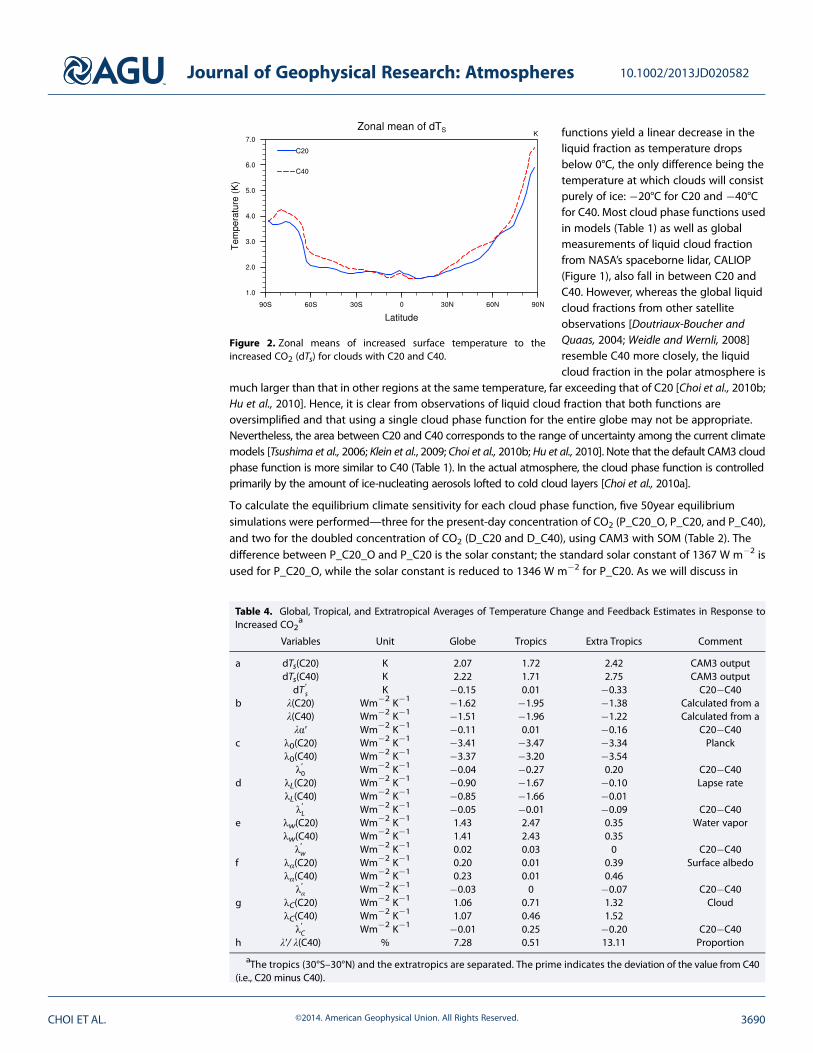
Figure 2. Zonal means of increased surface temperature to theincreased CO2 (dTs) for clouds with C20 and C40.
Table 4. Global, Tropical, and Extratropical Averages of Temperature Change and Feedback Estimates in Response toIncreased CO2
a
Variables Unit Globe Tropics Extra Tropics Comment
a dTs(C20) K 2.07 1.72 2.42 CAM3 outputdTs(C40) K 2.22 1.71 2.75 CAM3 outputdT ′
s K �0.15 0.01 �0.33 C20�C40b λ(C20) Wm�2 K�1 �1.62 �1.95 �1.38 Calculated from a
section 2.2, the purpose of adjustingthe solar constant in P_C20 is tominimize the difference between itsmodeled climate state and that ofP_C40, which thereby isolates theinfluence of cloud phase function.Thus, we will mainly use P_C20, insteadof P_C20_O. D_C20 minus P_C20 andD_C40 minus P_C40 represent theeffects of elevated CO2 concentrationfor the C20 and C40 functions,respectively. In addition, the differentclimate response to doubled CO2
concentration between C20 and C40 canbe represented by (D_C20 minus P_C20)minus (D_C40 minus P_C40). Weanalyzed the equilibrated climatology ofthe last 30 model years.
Table 3 summarizes the climate statesof the P_C20_O, P_C20, and P_C40experiments. The simulated global(extratropical) mean temperature forP_C20_O was much higher than thatfor P_C40 by ~1.74 K (2.29 K). This resultillustrates the strength of the impact ofcloud phase function on simulatedclimate state. The warmer climate forP_C20_O relative to P_C40 can beexplained by the fact that opticallythinner clouds allowmore SW radiationto reach the surface, whichconsequently lowers surface albedo inthe extratropics (by 0.9 and 1.0% fordirect and diffuse radiation,respectively). Note that at fixed total
water content, a liquid cloud is more reflective than an ice cloud, since ice crystals are relatively fewer andlarger than liquid water droplets. By the same token, an ice cloud will precipitate more quickly and efficientlythan a liquid cloud. Thus, converting a liquid cloud to an ice cloud implies a replacement of many small waterdroplets with few large ice crystals, which would reduce the lifetime and reflectivity of the cloud and increaseprecipitation (P_C20_O minus P_C40 in Table 3). As a consequence, the net global mean downward SWradiation for P_C20_O exceeds that of P_C40 by 6.66 and 5.54 Wm�2 at the top of the atmosphere (TOA) andsurface, respectively. In order to balance the additional absorbed SW radiation, the surface temperature inP_C20_O must be higher than that of P_C40. The resulting change in surface temperature may then induceother climate feedbacks.
To allow for a fair comparison in which the differences in climate feedbacks between the two experiments aresolely due to the different cloud phase functions, the global mean temperatures of P_C20 and P_C40 wereequalized by adjusting the solar constant. While it is not clear whether adjusting factors other than the solarconstant, for example, Q flux that represents seasonal deep water exchange and horizontal ocean heattransport [Collins et al., 2004] is more appropriate for this study, the advantage of adjusting the solar constantis that it avoids the issue of directly perturbing atmosphere and ocean coupling, which is intricately tied to climatesensitivity. We see in Table 3 that reduction of the solar constant (in P_C20) leads to lower surface temperature,fewer tropical clouds, less precipitation, less downward SW flux (mainly due to reduction of incident solarradiation), weaker SW cloud forcing, thicker sea ice, and higher surface albedo (see P_C20_Ominus P_C20).
Figure 3. (a and b) Spatial distribution of climate sensitivity in response toincreased CO2 (dTs) and (c) the difference.
Journal of Geophysical Research: Atmospheres 10.1002/2013JD020582
All of these changes seem to be physicallyconsistent with each another, and withthe results of Boer et al. [2005], who alsochanged the solar constant. We notethat the change in LW cloud forcing isfairly small.
Finally, Table 3 shows that reduction ofthe solar constant greatly reduces thedifference between the two present-dayclimates of P_C20 and P_C40 in manyimportant aspects such as the global-mean surface temperature,precipitation, net solar flux at TOA, sea-ice thickness, and surface albedo. Forthese properties, the differencesbetween P_C20 and P_C40 areapproximately 3�55% of the originaldifferences between P_C20_O andP_C40. However, differences in thesimulated cloud fraction and SW cloudradiative forcing increase slightly.
2.3. Calculation of Climate Feedbacks
Climate feedbacks are defined in termsof changes in global (or regional) mean
surface temperature Ts� �
, and changes in
radiative flux at the top of theatmosphere (R). For each cloud phasefunction, the equilibrium surface
temperatures, Ts , are calculated forpresent-day and doubled CO2
concentrations. The temperature
difference, dTs , between the doubledand the present-day CO2 concentrations
(i.e., D_C20 minus P_C20 for C20, and D_C40 minus P_C40 for C40) thus yields the equilibrium climate sensitivityfor an imposed radiative forcing due to the doubling of CO2 (3.35 Wm�2 from the calculation based on the initialchange in net downward radiative flux at TOA in the present model) [Gregory et al., 2004]. We define the total
climate feedback parameter, λ, to be the total derivative dR=dTs that can be expanded using the chain rule:
λ ¼ dR
dTs¼ ∑
i
∂R∂xi
dxidTs
(1)
where the last term in equation (1) indicates that the change in flux is due to not only changes in Ts but alsothe various auxiliary variables xi (e.g., lapse rate (L), cloud (C), water vapor (w), and albedo (α)) that areinfluenced by Ts. Equation (1) can be equivalently rewritten as
λ ¼ λ0 þ λL þ λC þ λw þ λα (2)
where
λ0 ¼ ∂R∂Ts
dTsdTs
þ ∂R∂T
dTsdTs
; (3a)
λL ¼ ∂R∂T
dT
dTs� ∂R∂T
dTsdTs
; (3b)
λi ¼ ∂R∂xi
dxidTs
for i ¼ C; w; α (3c)
Figure 4. Probability density function of climate sensitivity to theincreased CO2 (dTs) for a 2.8°-grid domain for clouds with C20 and C40.Forty bins of size 0.2 K are used. (a) The tropics (30°S–30°N) and (b) theextratropics (30°S–90°S and 30°N–90°N). The total number of grid pointsis 2816 for the tropics and 5376 for the extratropics. The probability iscalculated as the percentage of total grid points in each bin.
Journal of Geophysical Research: Atmospheres 10.1002/2013JD020582
are the climate feedback parametersassociated with the atmospheric variablexi (in units of Wm�2 K�1). The dxi anddTsare the differences in xi and global meansurface temperatures between thepresent-day and the doubled CO2
climate simulations, respectively. Thepartial derivatives ∂R/∂xi are called theradiative feedback kernels. This “radiativekernel method” developed by Soden andHeld [2006] has been widely used tocompute individual feedbacks in previousstudies [see, e.g., Shell et al., 2008; Jonkoet al., 2012]. In this study, the CAMradiative kernels are used [Shell et al.,2008]. The Planck response is representedas λ0, i.e., the negative feedbackassociated with the temperaturedependence of thermal emission. It iscalculated assuming uniform temperaturechange throughout the troposphere in theabsence of changes in lapse rate. It isexpressed as the sum of the surfacetemperature kernel and the atmospherictemperature (T) kernel at every level belowthe tropopause, both of which aremultiplied by dTs and normalized by dTs(equation (3a)). The tropopause is definedto be at 100 hPa at the equator and linearlyincreases with latitude until it reaches300 hPa at the poles [Soden and Held,2006; Jonko et al., 2012]. The lapse ratefeedback (λL) is computed as theproduct of the T kernel and the lapserate change (dT�dTs), normalized by dTs (equation (3b)). The sum λ0 + λL isreferred to as the “temperaturefeedback” (λT).
The water vapor and albedo feedbacks (λw and λα) are calculated by multiplying the water vapor and albedokernels by differences in the natural log of specific humidity and surface albedo between the doubled CO2
and present climate simulations, respectively (equations (3c) and (3d)). Due to nonlinearities in thecalculation of the kernel arising from complicated vertical overlap of clouds, λC is computed as the residualdifference between λ and other feedback parameters in equation (2). However, we note that this residualmethod of calculation for cloud feedback is a potential source of error in our calculations since otherfeedbacks may be dependent on cloud feedbacks themselves. Each λi is a function of latitude, longitude, andaltitude (except for surface albedo feedback). Global feedback parameters are calculated by integrating fromthe surface to the tropopause and averaging globally.
The change in the climate feedback parameters due to the cloud phase change from C40 to C20 is then
λ′ ¼ λ′0 þ λ′L þ λ′C þ λ′w þ λ′α (4)
where the primes indicate deviations from the feedback value of C40 (i.e., C20 minus C40).
The climate feedback parameters represented in equations (1) to (4) are calculated for the tropics andextratropics in this study. However, it should be borne in mind that the feedback parameter for a given regioncannot be directly compared to that for the globe or that for any other region.
Figure 5. Zonal mean of changes in relative humidity in response toincreased CO2 for clouds with C20 (a) and C40 (b). (c) The difference(C20 minus C40). The solid lines indicate zonally averaged temperaturesfor D_C20 (purple) and D_C40 (black); the dashed lines indicate zonallyaveraged temperatures for P_C20 (purple) and P_C40 (black).
Journal of Geophysical Research: Atmospheres 10.1002/2013JD020582
3. The Influence of Cloud PhaseComposition onClimate Feedbacks
The two cloud phase partitioningschemes, C20 and C40 (Figure 1), caninfluence cloud feedbacks in twoopposing ways. In the C20 scheme,clouds are purely composed of iceparticles at temperatures between�40°C and �20°C. Thus, one wouldexpect a stronger mixed-phase cloudresponse for C40 than for C20 attemperatures between �40°C and�20°C. However, the stronger mixed-phase cloud response for C40 may becounteracted by the more rapid changein liquid cloud fraction at temperatureswarmer than �20°C in the C20 scheme,where the liquid fraction decreases morerapidly with decreasing temperature. Attemperatures warmer than �20°C, onewould expect C20 to yield a strongercloud response induced by the CO2
warming. As a consequence, these twoopposing effects might compete indetermining the total cloud feedback.Since the cloud feedback is also stronglycoupled with other climate feedbackprocesses, substantial changes in themagnitude of various climate feedbacksare expected. In order to investigate howclimate feedbacks are altered, we shallbegin with discussing the equilibriumclimate sensitivity, which is a consequenceof climate feedbacks induced by warming.
Figure 2 shows the zonal mean surface temperature in response to increased CO2 concentration (dTs),
simulated for C20 (blue solid line) and C40 (red dashed line). dTs is generally larger at higher latitudes,reaching a maximum of ~ 7 K in the arctic. At most latitudes, dTs for C20 is lower than that for C40, with theexception of the equatorial region. In the extratropics, the dTs difference between C20 and C40 appears to bestatistically significant, as compared to the standard deviation of only 0.1 K of dTs resulting from interannualvariability [Danabasoglu and Gent, 2009]. As we will show later with our calculations of individual feedbacks(Table 4), this difference is largely caused by changes in the surface albedo and cloud feedbacks. In thetropics, however, changes in surface albedo feedback between C20 and C40 are negligible, because thetropical surface albedo feedback is close to zero in both simulations.
Figure 3 expands the zonally averaged dTs in Figure 2 to a latitude-longitude domain. dTs for C20 (Figure 3a) andC40 (Figure 3b) and the difference (C20 minus C40, Figure 3c) are displayed. As expected, the temperatureresponse, dTs is larger over the continents and lower over the ocean for a given latitude (Figures 3a and 3b). dTs isgenerally larger in C20 than in C40 in the tropics (red shade in Figure 3c), particularly in the tropical Pacific. On thecontrary, dTs is lower for C20 than for C40 (blue shading in Figure 3c) in the extratropics.
To characterize the frequency distribution of dTs, the probability density functions (PDFs) of grid point valuesof dTs for C20 and C40 are shown in Figure 4. In the tropics, the PDF of dTs for C20 (blue solid line) has a similardistribution to that for C40 (red dotted line); only slight differences between the PDFs of C40 and C20 exist.
Figure 6. The same as Figure 5, but for cloud fraction.
Journal of Geophysical Research: Atmospheres 10.1002/2013JD020582
However, analysis of the extratropics tells a different story. There are three peaks in the PDFs of dTs located atapproximately 2 K, 4 K, and 6 K. The first peak is shifted to the right, to higher temperatures for C40. Theprobability that dTs> 4K is generally larger in C40 than in C20, which reflects the stronger surface warming in C40in the northern hemisphere middle and high latitudes (see Figure 3). In summary, Figures 2–4 all consistentlyshow that dTs for C20 is lower than that for C40 in the extratropics (especially over continents), while thedifference is not as pronounced in the equatorial regions.
The feedback strengths corresponding to dTs for the globe, tropics, and extratropics were calculated fromequations (1) to (4) and are shown in Table 4. The change in climate feedbacks (C20minus C40) accounts for ~7.28%of the global feedback for C40 and is dominated by the change in the extratropics (13.11%, Table 4h). However, thelargest change in individual feedback strength occurs in tropical clouds (0.25Wm�2 K�1). This change in the sumoftropical cloud feedbacks is largely compensated by the change in Planck feedback (�0.27Wm�2 K�1) (Table 4c, g).Thus, although the net change in the total climate feedback is very small in the tropics (0.51% of the total)(Table 4h), it is clear that this is a result of compensation between larger changes in individual feedbacks. Theextratropical feedback change is associated with changes in all but the water vapour feedback (Table 4c to g).
The changes in the various feedback mechanisms can be understood by examining the vertical profiles ofresponses to the doubled CO2 concentration. When the atmospheric CO2 concentration increases, an increase insurface temperature follows, causing the temperature profile to rapidly adjust to a new radiative-convectiveequilibrium [Lindzen et al., 1982]. This is clearly shown in Figure 5 (solid line for present-day climate and dashed linefor doubled CO2 climate). Regions in the atmosphere with temperatures between the�40°C and 0°C are regionsin which the composition of mixed-phase clouds is affected by temperature changes.
These temperature adjustments can change relative humidity (RH), especially in the upper troposphere andlower stratosphere in the extratropics (colored contours in Figure 5). However, the upper level changes have a
Figure 7. The zonal mean of the liquid and ice cloud fraction profile in response to the increased CO2 for clouds with(a and b) C20 and (c and d) C40. The difference (C20 minus C40) is shown for (e) liquid and (f) ice cloud fraction, respectively.The solid lines indicate zonally averaged temperatures for D_C20 (purple) and D_C40 (black); the dashed lines indicate zonallyaveraged temperatures for P_C20 (purple) and P_C40 (black).
Journal of Geophysical Research: Atmospheres 10.1002/2013JD020582
negligible effect on feedback because the concentration of water vapor at that level is low. In the mid- and lowertroposphere, most of the change in RH is largest in the tropics. Interestingly, the pattern of the tropical tropopauseRH response is complex and shows large changes of opposite signs for different heights (Figures 5a and 5b),likely due to changes in shallow and deep convection (Figure 6). Despite this complicated vertical response ofRH, the vertically integrated specific humidity in the tropics in response to warming for C20 and C40 are nearlyequal. This explains why the water vapor feedback was virtually unchanged (Table 4e).
The cloud fraction response to doubled CO2 concentration (hereafter dAc) is shown in Figure 6. dAc for mixed-phase clouds (between �40°C and 0°C) is generally negative except at a few altitudes in the tropics(Figures 6a and 6b). In both C20 and C40, there is a strong reduction of tropical high clouds in response todoubled CO2 concentration. These high clouds have the potential to allow more SW radiation into thetropical atmosphere, which can explain the positive tropical cloud feedback in the model (Table 4g). Incontrast, there is an increase in high clouds above 300 hPa in the entire extratropics and a decrease of lowclouds around 850 hPa in the midlatitudes in response to the doubled CO2 concentration in both C20 andC40. This may act to increase trapping of LW radiation and penetration of SW radiation to the surface, whichexplains the positive extratropical cloud feedback in the model (Table 4g). As we will show in Figure 10, theSW responses dominate the longwave (LW) responses in general.
The relationship between cloud feedback and cloud phase function can be inferred from (Figure 6c). dAc(C20)minus dAc(C40) for ice-phase clouds (around�40°C level) is positive. In contrast, dAc(C20) minus dAc(C40) forcold mixed-phase clouds (around �20°C level) is negative. The contributions of liquid (a, c, e) and ice cloudfractions (b, d, f ) to the total cloud fractions (Figure 6) are displayed in Figure 7. We see that the response ofice cloud fraction to doubling of CO2 (Figures 7b and 7d) is more similar to the total cloud fraction in Figure 6than the water cloud fraction (Figures 7a and 7c). Between �40°C and 0°C, the sign of the change is theopposite between liquid- and ice-phase cloud fractions (Figure 7e versus Figure 7f). Overall, it can be said thatthe pattern of the total cloud fraction change is consistent with the changes in liquid-phase cloud fractionabove 0°C and ice-phase cloud fraction below 0°C. Note that all of the above effects strongly influence cloud
Figure 8. The same as Figure 7, but for in-cloud liquid water path and ice water path.
Journal of Geophysical Research: Atmospheres 10.1002/2013JD020582
feedback change. While the changein cloud feedback strength is notreadily identified in Figures 6 and 7,the results in Table 4g indicate thatthe tropical cloud feedbackstrengthens in C20, while theextratropical cloud feedback weakensrelative to C40.
The responses of the in-cloud liquidand ice water paths (LWP and IWP) tothe changes in cloud phasecomposition are other factors thatcan alter cloud feedback becauseLWP and IWP strongly influence theemissivity and reflectivity of mixed-phase clouds. The LWP and IWP arecalculated as grid-mean cloud waterpaths (CWP) weighted by liquid- andice-phase cloud fractions,respectively; LWP=CWP(1 � Ai) / Acand IWP=CWP ·Ai / Ac, where Ai is theice cloud fraction. In general, themodel-simulated LWP changes muchmore than IWP (Figure 8). Changes inLWP are generally positive for mixed-phase clouds (between �40°C and0°C), while they are negative for warmclouds (between 0°C and 20°C) inresponse to doubled CO2
concentration (Figures 8a and 8c).The reduction of LWP for warmclouds is consistent with thereduction of warm-cloud fraction(compare Figures 7 and 8). On theother hand, changes in IWP arepositive between �40°C and �20°Cand negative between�20°C and 0°C
in response to doubled CO2 concentration (Figures 8b and 8d). The ratio of LWP to IWP has an importantimplication. Comparing Figures 8a and 8b (or Figures 8c and 8d), an increase in LWP and a decrease in IWP areevident for mixed-phase clouds between�20°C and 0°C. This means that these clouds may become brighter andreflect more SW radiation in response to doubled CO2 concentration. This LWP/IWP effect alone would yield anegative cloud feedback. However, Table 4g shows a positive overall cloud feedback in CAM3. This implies that theLWP/IWP effect is secondary to the cloud fraction effect in determining cloud feedback strength.
As for the difference between C20 and C40, Figure 8e shows that above (below) the �20°C isotherm, LWPincreases (decreases) for C20 to a smaller extent than for C40. A similar but smaller change in IWP is alsofound at a slightly higher altitude (Figure 8f). These results indicate that both IWP and LWP generally covarybut that a decrease in the LWP/IWP ratio in C20 relative to C40 can be expected close to the�20°C isotherm.This decrease in LWP/IWP ratio would lead to a decrease in SW cloud albedo, possibly intensifying thepositive cloud feedback in the tropics (Table 4g).
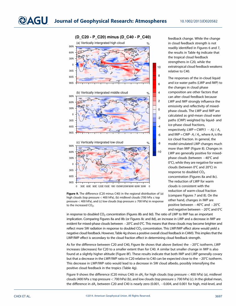
Figure 9 shows the difference (C20 minus C40) in dAc for high clouds (top pressure< 400 hPa) (a), midlevelclouds (400 hPa ≤ top pressure< 700 hPa) (b), and low clouds (top pressure ≥ 700 hPa) (c). In the global mean,the difference in dAc between C20 and C40 is nearly zero (0.001, �0.004, and 0.001 for high, mid-level, and
Figure 9. The difference (C20 minus C40) in the regional distribution of (a)high clouds (top pressure< 400 hPa), (b) midlevel clouds (700 hPa ≤ toppressure< 400 hPa), and (c) low clouds (top pressure ≥ 700 hPa) in responseto the increased CO2.
Journal of Geophysical Research: Atmospheres 10.1002/2013JD020582
low clouds, respectively); however,strong regional variability does exist.The difference in dAc for high cloudsis more pronounced in the tropicsthan in the extratropics; thedifference in dAc for mid-level cloudsis mostly negative; the difference indAc for low clouds is mostly positiveover the northern hemisphericcontinents. The positive difference forlow clouds would imply less absorbedSW radiation in the atmosphere.
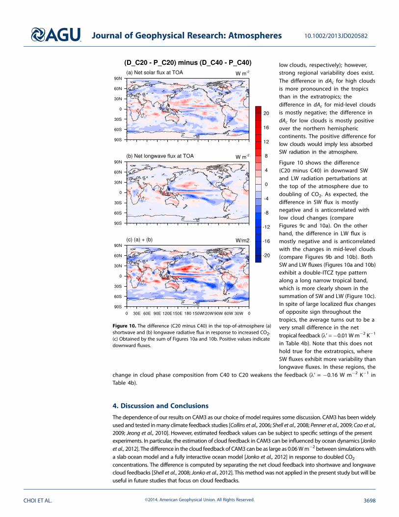
Figure 10 shows the difference(C20 minus C40) in downward SWand LW radiation perturbations atthe top of the atmosphere due todoubling of CO2. As expected, thedifference in SW flux is mostlynegative and is anticorrelated withlow cloud changes (compareFigures 9c and 10a). On the otherhand, the difference in LW flux ismostly negative and is anticorrelatedwith the changes in mid-level clouds(compare Figures 9b and 10b). BothSW and LW fluxes (Figures 10a and 10b)exhibit a double-ITCZ type patternalong a long narrow tropical band,which is more clearly shown in thesummation of SW and LW (Figure 10c).In spite of large localized flux changesof opposite sign throughout thetropics, the average turns out to be avery small difference in the nettropical feedback (λ′ =�0.01Wm�2 K�1
in Table 4b). Note that this does nothold true for the extratropics, whereSW fluxes exhibit more variability thanlongwave fluxes. In these regions, the
change in cloud phase composition from C40 to C20 weakens the feedback (λ′ = �0.16 W m�2 K�1 inTable 4b).
4. Discussion and Conclusions
The dependence of our results on CAM3 as our choice of model requires some discussion. CAM3 has been widelyused and tested inmany climate feedback studies [Collins et al., 2006; Shell et al., 2008; Penner et al., 2009; Cao et al.,2009; Jeong et al., 2010]. However, estimated feedback values can be subject to specific settings of the presentexperiments. In particular, the estimation of cloud feedback in CAM3 can be influenced by ocean dynamics [Jonkoet al., 2012]. The difference in the cloud feedback of CAM3 can be as large as 0.06Wm�2 between simulationswitha slab ocean model and a fully interactive ocean model [Jonko et al., 2012] in response to doubled CO2
concentrations. The difference is computed by separating the net cloud feedback into shortwave and longwavecloud feedbacks [Shell et al., 2008; Jonko et al., 2012]. This method was not applied in the present study but will beuseful in future studies that focus on cloud feedbacks.
Figure 10. The difference (C20 minus C40) in the top-of-atmosphere (a)shortwave and (b) longwave radiative flux in response to increased CO2.(c) Obtained by the sum of Figures 10a and 10b. Positive values indicatedownward fluxes.
Journal of Geophysical Research: Atmospheres 10.1002/2013JD020582
The present study has shown that climate feedbacks are highly sensitive to temperature-dependent cloudphase functions. Here, we have used two different cloud phase functions, C20 and C40, to reflect thevariability of cloud phase dependence on temperature found among various models. In the C20 (C40)experiment, all liquid droplets are converted to ice crystals below �20°C (�40°C), so that both liquid and iceclouds co-exist at temperatures between 0°C and �20°C (�40°C). By adjusting the solar constant, the globalannual mean temperatures in C20 and C40 were set to be similar. Doing otherwise would cause a significantmean surface temperature difference of ~1.7°C between C20 and C40, leading to different climatologies inprecipitation, surface albedo, etc. between the two cloud phase partitioning schemes that would not allowfor fair comparisons between C20 and C40.
Our simulations show that changing the cloud phase function from C40 to C20 alters the cloud feedback inthe tropics by 0.25 Wm�2 K�1 and in the extratropics by�0.20 Wm�2 K�1, the temperature feedback in thetropics by �0.28 W m�2 K�1 and in the extratropics by 0.11 W m�2 K�1, and the albedo feedback in theextratropics by �0.07 W m�2 K�1. Due to compensation of feedback changes, the net change in globalclimate feedback is 7.3% of the total feedback (�0.11 W m�2 K�1) and is dominated by changes in theextratropics. The influence of the solar constant on feedbacks is negligible. These results suggest thatadjustment of the cloud phase function affects all types of feedbacks (with the least effect on water vaporfeedback). Although there are substantial differences in the individual climate feedbacks between the twocloud phase partitioning schemes, cancellation of the various feedbacks resulted in a small net change in theoverall climate feedback. However, should the climate system be very sensitive to an increase in CO2, even asmall change in the net climate feedback induced by changes in the cloud phase partitioning scheme wouldlead to a large bias in climate prediction [Roe and Baker, 2007].
As revealed by satellite observations, significantly different regional and transient variations of the cloudphase function occur naturally mainly due to the role of dust aerosols [Choi et al., 2010a]. A smaller liquidcloud fraction was generally observed at lower latitudes and in regions with abundant dust aerosols in coldcloud layers. In light of the complex regional and vertical distributions of liquid cloud fraction, this studyimplies that recent investigations with more sophisticated modeling of aerosol-cloud interactions are of vitalimportance for accurate simulations of climate feedbacks, and by extension, climate prediction.
ReferencesBoer, G. J., K. Hamilton, and W. Zhu (2005), Climate sensitivity and climate change under strong forcing, Clim. Dyn., 24, 685–700.Bretherton, C. S., and S. Park (2009), A new moist turbulence parameterization in the Community Atmosphere Model, J. Clim., 22, 3422–3448.Cao, L., G. Bala, K. Caldeira, R. Nemani, and G. Ban-Weiss (2009), Climate response to physiological forcing of carbon dioxide simulated by the coupled
Community Atmosphere Model (CAM3.1) and Community Land Model (CLM3.0), Geophys. Res. Lett., 36, L10402, doi:10.1029/2009GL037724.Choi, Y.-S., R. S. Lindzen, C.-H. Ho, and J. Kim (2010a), Space observations of cold-cloud phase change, Proc. Natl. Acad. Sci. U.S.A., 107,
11,211–11,216.Choi, Y.-S., C.-H. Ho, S.-W. Kim, and R. S. Lindzen (2010b), Observational diagnosis of cloud phase in the winter Antarctic atmosphere for
parameterizations in climate models, Adv. Atmos. Sci., 27, 1233–1245.Collins, W. D., et al. (2004), Description of the NCAR Community Atmosphere Model (CAM 3.0), National Center for Atmospheric Research,
Boulder, Colo.Collins, W. D., P. J. Rasch, B. A. Boville, J. J. Hack, J. R. McCaa, D. L. Williamson, B. P. Briegleb, C. M. Bitz, S.-J. Lin, and M. Zhang (2006),
The Formulation and atmospheric simulation of the Community Atmosphere Model version 3 (CAM3), J. Clim., 19, 2144–2161.Danabasoglu, G., and P. R. Gent (2009), Equilibrium climate sensitivity: Is it accurate to use a slab ocean model?, J. Clim., 22, 2,494–2,499.Del Genio, A. D., M.-S. Yao, W. Kovari, and K. W. Lo (1996), A prognostic cloud water parameterization for global climate models, J. Clim., 9,
270–304.Doutriaux-Boucher, M., and J. Quaas (2004), Evaluation of cloud thermodynamic phase parameterizations in the LMDZ GCM by using
POLDER satellite data, Geophys. Res. Lett., 31, L06126, doi:10.1029/2003GL019095.Ebert, E. E., and J. A. Curry (1992), A parameterization of ice cloud optical properties for climate models, J. Geophys. Res., 97, 3831–3836.Gettelman, A., X. Liu, D. Barahona, U. Lohmann, and C. Chen (2012), Climate impacts of ice nucleation, J. Geophys. Res., 117, D20201,
doi:10.1029/2012JD017950.Gregory, J. M., W. J. Ingram, M. A. Palmer, G. S. Jones, P. A. Stott, R. B. Thorpe, J. A. Lowe, T. C. Johns, and K. D. Williams (2004), A new method
for diagnosing radiative forcing and climate sensitivity, Geophys. Res. Lett., 31, L03205, doi:10.1029/2003GL018747.Ho, C.-H., M.-D. Chou, M. Suarez, and K.-M. Lau (1998), Effect of ice cloud on GCM climate simulations, Geophys. Res. Lett., 25, 71–74.Hu, Y., S. Rodier, K. Xu, W. Sun, J. Huang, B. Lin, P. Zhai, and D. Josset (2010), Occurrence, liquid water content, and fraction of supercooled
water clouds from combined CALIOP/IIR/MODIS measurements, J. Geophys. Res., 115, D00H34, doi:10.1029/2009JD012384.Intergovernmental Panel on Climate Change (2007), Climate Change 2007: The Physical Science Basis. Contribution ofWorking Group I to the Fourth
Assessment Report of the Intergovernmental Panel on Climate Change, edited by S. Solomon et al., Cambridge Univ. Press, Cambridge.Jeong, S.-J., C.-H. Ho, T.-W. Park, J. Kim, and S. Levis (2010), Impact of vegetation feedback on the temperature and its diurnal range over the
Northern Hemisphere during summer in a 2 × CO2 climate, Clim. Dyn., doi:10.1007/s00382-010-0827.Jonko, A. K., K. M. Shell, B. M. Sanderson, and G. Danabasoglu (2012), Climate feedbacks in CCSM3 under changing CO2 forcing. Part II:
Variation of climate feedbacks and sensitivity with forcing, J. Clim., 26, 2784–2795.
AcknowledgmentsThis study was supported by theNational Research Foundation of Korea(NRF) grant funded by the Korea gov-ernment (MSIP) (2009-0083527) and theKorea Meteorological AdministrationResearch and Development Programunder grant CATER 2012–3064. Theauthors thank R. S. Lindzen for valuablecomments. The radiative kernels for thispaper are available at K. M. Shell’shomepage (http://people.oregonstate.edu/~shellk/kernel.html). Kernel files:Kernels.zip. The CALIOP data are avail-able online at the NASA LangleyAtmospheric Sciences Data Centerwebsite (https://eosweb.larc.nasa.gov/order-data).
Journal of Geophysical Research: Atmospheres 10.1002/2013JD020582
Klein, S. A., et al. (2009), Intercomparison of model simulations of mixed-phase clouds observed during the ARM Mixed-Phase Arctic CloudExperiment. I: Single-layer cloud, Q. J. R. Meteorol. Soc., 135, 976–1002.
Le Treut, H., and Z. X. Li (1991), Sensitivity of an atmospheric general circulation model to prescribed SST changes: Feedback effects asso-ciated with the simulation of cloud optical properties, Clim. Dyn., 5, 175–187.
Lee, M.-I., I.-S. Kang, J.-K. Kim, and B. E. Mapes (2001), Influence of cloud-radiation interaction on simulating tropical intraseasonal oscillationwith an atmospheric general circulation model, J. Geophys. Res., 106, 14,219–14,233.
Li, Z. X., and H. Le Treut (1992), Cloud-radiation feedbacks in a general circulation model and their dependence on cloud modelingassumptions, Clim. Dyn., 7, 133–139.
Lindzen, R. S., and Y.-S. Choi (2009), On the determination of climate feedbacks from ERBE data, Geophys. Res. Lett., 36, L16705, doi:10.1029/2009GL039628.
Lindzen, R. S., and Y.-S. Choi (2011), On the observational determination of climate sensitivity and its implications, Asia-Pac. J. Atmos. Sci.,47(4), 377–390.
Lindzen, R. S., A. Y. Hou, and B. F. Farrell (1982), The role of convective model choice in calculating the climate impact of doubling CO2,J. Atmos. Sci., 39, 1189–1205.
Liou, K. N. (2002), Presentation of a unified theory for light scattering by ice crystals, in An Introduction to Atmospheric Radiation, 2nd ed.,pp. 228–234, Elsevier, New York.
Lohmann, U., and C. Hoose (2009), Sensitivity studies of different aerosol indirect effects in mixed-phase clouds, Atmos. Chem. Phys., 9,8917–8934.
Mason, B. J. (1957), The Physics of Clouds, Clarendon Press, Oxford.Meehl, G. A., et al. (2007), Global climate projections, in Climate Change 2007: The Physical Science Basis. Contribution of Working Group I to the Fourth
Assessment Report of the Intergovernmental Panel on Climate Change, edited by S. Solomon et al., pp. 749–845, Cambridge Univ. Press, Cambridge.Oleson, K. W., et al. (2004), Technical description of the Community Land Model (CLM), NCAR Tech. Note, NCAR/TN-461+STR.Penner, J. E., Y. Chen, M. Wang, and X. Liu (2009), Possible influence of anthropogenic aerosols on cirrus cloud and anthropogenic forcing,
Atmos. Chem. Phys., 9, 879–896.Pruppacher, H., and J. Klett (1997), Microphysics of Clouds and Precipitation, Kluwer Acad., Neth.Roe, G. H., and M. B. Baker (2007), Why is climate sensitivity so unpredictable?, Science, 318, 629.Senior, C. A., and F. B. Mitchell (1993), Carbon dioxide and climate: The impact of cloud parameterization, J. Clim., 6, 393–418.Shell, K. M., J. T. Kiehl, and C. A. Shields (2008), Using the radiative kernel technique to calculate climate feedbacks in NCAR’s Community
Atmospheric Model, J. Clim., 21, 2269–2282.Smith, R. N. (1990), A scheme for predicting layer clouds and their water content in a general circulation model, Q. J. R. Meteorol. Soc., 116,
435–460.Soden, B. J., and T. M. Held (2006), An assessment of climate feedbacks in coupled ocean–atmosphere models, J. Clim., 19, 3354–3360.Song, X., G. J. Zhang, and J. L. F. Li (2012), Evaluation of microphysics parameterization for convective clouds in the NCAR Community
Atmosphere Model CAM5, J. Clim., 25, 8568–8590.Storelvmo, T., J. E. Kristjánsson, and U. Lohmann (2008), Aerosol influence on mixed-phase clouds in CAM-Oslo, J. Atmos. Sci., 65, 3214–3230.Sundqvist, H. (1988), Parameterization of condensation and associated clouds in models for weather prediction and general circulation
simulation, in Physically-Based Modeling and Simulation of Climate and Climate Change, vol. 1, edited by M. E. Schlesinger, pp. 433–461,Kluwer Acad, Dordrecht, Neth.
Tsushima, Y., M. J. Webb, K. D. Williams, B. J. Soden, M. Kimoto, Y. Tsushima, S. Emori, N. Andronova, B. Li, and T. Ogura (2006), Importance ofthe mixed-phase cloud distribution in the control climate for assessing the response of clouds to carbon dioxide increase: A multi-modelstudy, Clim. Dyn., 27, 113–126.
Webb, M. J., et al. (2006), On the contribution of local feedback mechanisms to the range of climate sensitivity in two GCM ensembles, Clim.Dyn., 27, 17–38.
Weidle, F., and H. Wernli (2008), Comparison of ERA40 cloud top phase with POLDER-1 observations, J. Geophys. Res., 113, D05209,doi:10.1029/2007JD009234.
Journal of Geophysical Research: Atmospheres 10.1002/2013JD020582