INFORMATION TO USERS This reproduction was made from a copy of a document sent to us for microfilming. While the most advanced technology has been used to photograph and reproduce this document, the quality of the reproduction is heavily dependent upon the quality of the material submitted. The following explanation of techniques is provided to help clarify markings or notations which may appear on this reproduction. 1. The sign or "target" for pages apparently lacking from the document photographed is "Missing Page(s)". If it was possible to obtain the missing page(s) or section, they are spliced into the film along with adjacent pages. This may have necessitated cutting through an imageand duplicating adjacent pages to assure complete continuity. 2. When an image on the film is obliterated with a round black mark, it is an indication of either blurred copy because of movement during exposure, duplicate copy, or copyrighted materialsthat should not have been filmed. For blurred pages, a good image of the page can be found in the adjacent frame. If copyrighted materials were deleted, a target note will appear listing the pages in the adjacent frame. 3. When a map, drawing or chart, etc., is part of the material being photographed, a definite method of "sectioning" the material has been followed. It is customary to begin filming at the upper left hand corner of a large sheet and to continue from left to right in equal sections with small overlaps. If necessary, sectioning is continued again-beginning below the first row and continuing on until complete. 4. For illustrations that cannot be satisfactorily reproduced by xerographic means, photographic prints can be purchased at additional cost and inserted into your xerographic copy. These prints are available upon request from the Dissertations Customer Services Department. 5. Some pages in any document may have indistinct print. In all cases the best available copy has been filmed. MicrOfilms International 300 N. Zeeb Road Ann Arbor, MI48106
Transcript
INFORMATION TO USERS
This reproduction was made from a copy of a document sent to us for microfilming.While the most advanced technology has been used to photograph and reproducethis document, the quality of the reproduction is heavily dependent upon thequality of the material submitted.
The following explanation of techniques is provided to help clarify markings ornotations which may appear on this reproduction.
1. The sign or "target" for pages apparently lacking from the documentphotographed is "Missing Page(s)". If it was possible to obtain the missingpage(s) or section, they are spliced into the film along with adjacent pages. Thismay have necessitated cutting through an image and duplicating adjacent pagesto assure complete continuity.
2. When an image on the film is obliterated with a round black mark, it is anindication of either blurred copy because of movement during exposure,duplicate copy, or copyrighted materials that should not have been filmed. Forblurred pages, a good image of the page can be found in the adjacent frame. Ifcopyrighted materials were deleted, a target note will appear listing the pages inthe adjacent frame.
3. When a map, drawing or chart, etc., is part of the material being photographed,a definite method of "sectioning" the material has been followed. It iscustomary to begin filming at the upper left hand corner of a large sheet and tocontinue from left to right in equal sections with small overlaps. If necessary,sectioning is continued again-beginning below the first row and continuing onuntil complete.
4. For illustrations that cannot be satisfactorily reproduced by xerographicmeans, photographic prints can be purchased at additional cost and insertedinto your xerographic copy. These prints are available upon request from theDissertations Customer Services Department.
5. Some pages in any document may have indistinct print. In all cases the bestavailable copy has been filmed.
Univer~MicrOfilms
International300 N. Zeeb RoadAnn Arbor, MI48106
8429308
Lee, Kwangsuck
EFFECTS OF FARM SIZE AND LAND TENURE ON THE ECONOMICEFFICIENCY OF RICE FARMING IN KOREA
University of Hawaii
UniversityMicrofilms
International 300N. Zeeb Road, Ann Arbor, MI48106
PH.D. 1984
EFFECTS OF .FARM SIZE AND LAND TENURE ON
THE ECONOMIC EFFICIENCY OF RICE FARMING IN KOREA
A DISSERTATION SUBMITTED TO THE GRADUATE DIVISION OF THEUNIVERSITY OF HAiAII IN PARTIAL FULFILLMENT
OF rHE REQUIREMENTS FOR THE DEGREE OF
DOCTOR OF PHILOSOPHY
IN AGRICULTURAL AND RESOURCE ECONOMICS
AUGUST 1984
By
Kwangsuck Lee
Dissertation Committee:
Hiroshi Yamauchi, ChairmanHarold L. BakerJack R. Davidson
Gary R. ViethYong-ho Choe
ACKBOiLEDGEMEHTS
There are no adequate wo~ds to fully acknowledge and
thank all who taught, guided, sup~orted, and encouraged me
in the course of successfully completing my studies. First
of all, I am thankful and deeply indebted to my dissertation
committee: My committee chairman, Dr. Hiroshi Yamauchi, who
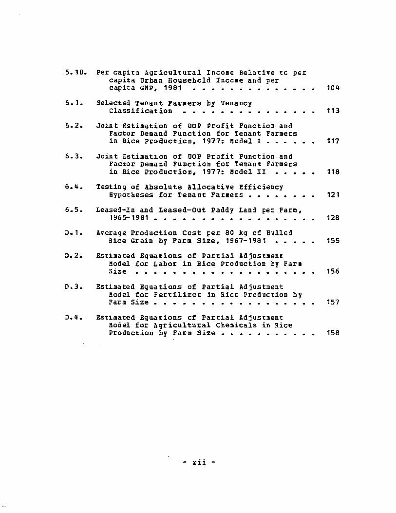
0.1. Cost-Volume Scat~er Diagram in Dice Production 159
- xiii -
Chapter I
IB7RODUCTIOH
1.1 BACKGROUND Of THE PROBLE"
In the modern economic growth of nations, the rela~ive
decline of agriculture in the overall economies raises the
impor~an~ ques~ion on ~he role of agricul~ure in sus~aining
economic growth. A typical case of such an occurrence is,
within the la~ two decades, ~be ra~id transforma~ion of
Korea from a primarily agrarian to a mixed-industrial
economy.
The structure of Korean agriculture has presently been
considerably changed. The nUKber of farms and ~be rural
population have been sharply reduced as migraticn from
rural ~o urban areas con~inues. ~his is due primarily ~o
rapid economic growth since the late 1960s that has brought
for~h urbaniza~ion and indus~rializa~ion. Prom 1965 ~o
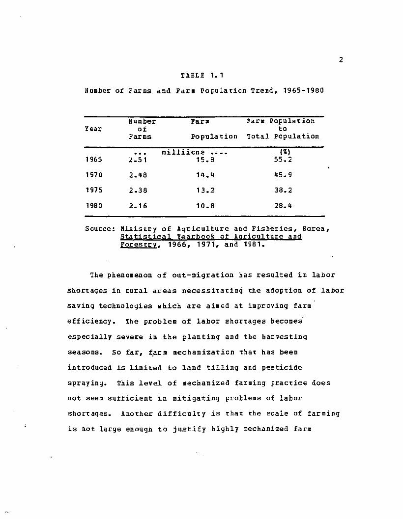
1980, the number of farms decreased by 14 percen~, while ~he
rural population declined 32 ~ercent, dropping from 55
percen~ of the ~o~al population in 1965 to 28 percen~ in
1980 (Table 1.1).
- 1 -
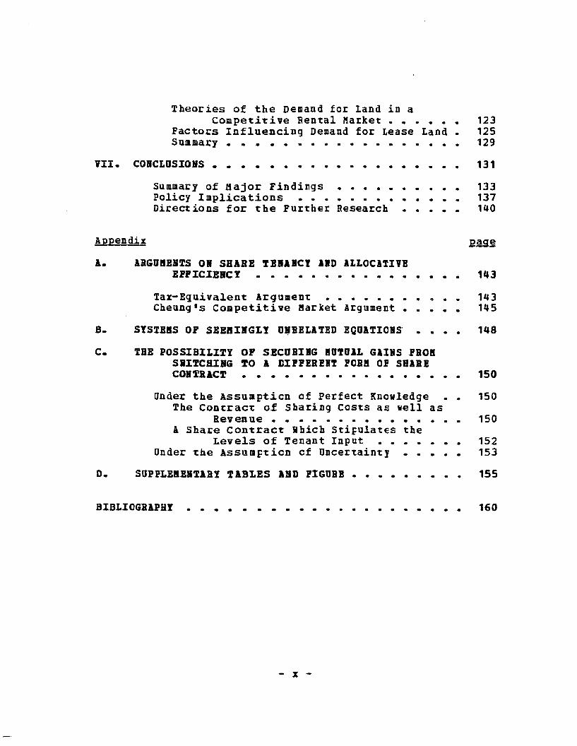
2
TABLE 1.1
Number of Farms and Far. POFulaticn Trend, 1965-1980
Year
1965
1970
1975
1980
Number Farm Parm Popula1:ionof to
Parms Popula tion 'Iotal Population
.. . milliicns .... (%)2.51 15.8 55 .. 2
2.48 14.4 45.9
2.38 13.2 38.2
2 .. 16 10.8 28.4
Source: Ministry of Aqriculture and Fisheries, Rorea,Statistical Yearbook of Agriculture andForestry, 1966,1971, and 1981.
'Ihe phenomenon of out-migration has resulted in labor
shortages in rural areas necessitating the adoption of labor
saving technologies which are aimed at improving farm
efficiency. The problem of labor shortages become~
especially severe in the planting and the harvesting
seasons. So far, ~arm mechanization ~hat has been
introduced is limited to land tilling and pesticide
spraying. This level of mechanized farming Fractice does
not seem sufficient in mitigating ~roblems of labor
shortaqes. Another difficulty is that the scale of farming
is not large enough to justify highly mechanized farm
3
~echnologies. On ~he o~ber hand, farm lands which cannot be
managed by remaining family mempers ~end to be fully or
partially leased out. Tenancy Fractices can also be created
when the amoun~ of land supplied by migrating farmers cannot
be purchased by farm ers who rema ill in rural area. In
addition, some urban bound farmers want to keep their land
under tenancy because land is the only property on which
they can rely in the event of bankruFtcy in urban living.
As a result, tenant farming has become an increasing trend.
According to the 1970 Agricultural Census, about 34 percent
of total farms were iden~ified as full or partial tenant
farms.
Current land law in Korea originates in the land reform
law of 1950. Legally, farm size is limited to a 3 hectare
ceiling and tenancy is prohibited. A conflict has arisen
between the actual farming structure and the land law in
Korea. Accordingly, the legal frcvision limiting acreage
and prohibiting tenancy haVE become ccntroversial issues.
Indeed, the tWO problems are no~ independent of each other,
but, rather, they are intervined.
1.1.1 The Proble. of Fara Size
Farm size pr~blem has been raised since 1968 when ~he
4
Korean government sugges~ed a relaxation of 3 hectare land
ceiling. It was argued that expansion of farming scale is
necessary to economically use labor-saving farm machines. 1
This is believed to be a cri~ical condition for modernizing
Korean aqriculture. In addition, it is insisted that the
farm size limitations be removed in order to develoF a
self-supporting farming structure through scale expansion
which would result in balanced growth between the
ag.ricultural sector and the non-agricultural sector. 2
The opposing argument is that if ~he land size ceiling
were removed, then urban capital wQuld Furchase most farm
land, creating extreme land concentraticn or a land
aristocracy. Thus this would lead to the collapse of the
small peasant-farming system. When the landless peasants
become tenants, a feudal tenancy system would te revived or
unemploymen t would spread in the rural area. The argument
1 The peak of labor shortage Froblem in producing ricereaches in the seasons of rice transFlanting andharvesting. A research reports that 7.7 hectares and 5.7hectares of land are reguired to use a rice-transFlan~er
and a cutter, respectively, at least meeting a treat-evenof l:enefit and cost, as cited by Oh (p, 63).
2 Oh (pp. 160-161) estimates a required land size per farmfor assuring per capi~a farm income egual ~o 60 percent ofGNP per capita is at least 4.0 hectares in 1991 under theassumption that GNP per capita will reach $ 4,000 in ~ha~
year.
5
concludes that ultimately food producticn wculd te
drastically reduced due to decreases in prcductivity.
1.1.2 Tenancy Prob1ea
those who advocate the legalizaticn of tenancy
practices have argued that farm size can be flexibly
adjusted through a rental system when a farmer needs to
expand his farming scale. This argument also takes into
consideration the favorable bargaining power of tenants as
the labor shortage tends to favor tenants when entering into
rental negotiations. Thus it precludes any possitility of
re-creating a traditional tenancy system and a polarization
of land holdings. In addi~ion, when the land, made
available by an out-migration, cannot be purchased ty other
farmers in the rural communi~y, the legal ccnstraint on the
tenancy practice loses its efficacy. therefore, the
prevailing practices of disguised tenancy that presently
exiSt would be less reasonat1e or less efficient than if the
tenancy system would be institu~ionally allcwed.
Others who are in opposition to these arguments hold
pessimistic views on the open tenancy system. They arque
that currently existing tenancy practices are not much
differen~ from those of high rental contracts. thUS, if
tenancy is legally supported, then the relationshiF between
6
landlords and tenants will certainly tecome that of a
semi-feudal or feudal ~enancy system. Onder these
conditions, investment would not be made in land
improvements, and land u~ilization and productivity would
decrease.
1.2 RESEARCH PROBLEft
ihe arguments concerning the farm size and land ~enure
system in Korea have been continued since the late 1960s.
However, the problems and dis~utes have remained almost
unchanged. Neither argument is sufficiently strong to
resolve the issue, and more em~irical analysis with respect
to socia-economic concerns are needed.
In facing the issue cf appropriate farm scale in Korean
agriculture, the following two areas must be addressed: (1)
the question of economic efficiency under the continuing
farm size limitation of 3 hectares; and (2) the question of
the expected economic efficiency under the assum~ticn of no
legal barriers to size, and the viability of farms in
relation to sizes.
In fact, most empirical analyses of the effect of farm
size on economic efficiency in Korea might give answers to
the first question. Even though there are some farms
CUltivating more than 3 hectares, they a~e not completely
7
free cf legal constraints. Thus, they cannot be regarded as
operating large scale farms like those found in more
developed countries such as the United States and canada.
Hence, farm size analysis with the em~irical data in Korea
would suggest a direction for a struc~ural adjustment under
the assumption that the present legal constraint on the farm
size will not change.
The second guestion is more conceptual than the first.
Evidence on the level of econcmic efficiency of farms
cultivating more than three hectares is difficult to obtain.
However, efficiency in those faxms must be addressed, if
only in conceptual terms, if we are to find an appropriate
farming scale. Formulation of a methodology for estimating
efficient farm scale may be of particular benefit in
discussing the economic implications of continued use of the
three hectare legal limit on farm size. Moreover, the
viability of farms of different sizes is an important
question when determining the balanced-income level be~ween
agricultural and non-agricultural sectors.
!ven though tenancy is prohibited by the land law,
excluding some exemptions,3 the tenancy practices are a
known fact. Data on tenanted land, and the rents paid, are
3 When farmers are unable to operate their farms due todisease, education, military service~ and so ferth~ theycan rent OUt their land ~o ether farmers fer a shcrtperiod.
8
collected and ~ublished by ~hE governmen~. This imFlies
that the tenancy cannot be strongly controlled by the
current Korean land law.
the effeCt of ~enancy Frac~ices on econcmic efficiency
in agriculture is an important guestion. Resource
allocation under tenancy, especially share tenancy, has been
considered both efficient and inefficient in recent
theoretical discussion of the Frotlem (Cheung 1969a: Ip and
Stahl). If we can understand the level of resource
allocation under share tenancy, then we can Frovide policy
implications for the possible fcrms of rental contracts.
1.3 RICB II KORBA. BCOIOII!
Rice is the most important single crop in the Korean
economy in terms of bo~h food Froduction and consumption.
Rice is planted on most paddy fields, which eccuFied 59
percent of the total cul~iva~ed area in 1980. 4 For farm
households, rice is a major product determining farm income
because of its predominance in the productien pattern. In
1980, rice provided about 49 Fercent of the average gross
farm receipts. 5 Rice is also accoun~ed for 35 percen~ of
total food consumption in 1979 (Kim and Jeo, F. 3). This
4 Kinistry of Agriculture & Fisheries, Korea, StatisticalYearbook of Aoriculture and Forestrv~ 1981.
5 Ibid.
9
study will consider rice farming to be the problem area for
the examination of economic efficiency in rela~ion to farm
size and land tenure.
Korean rice farming has experienced a number of changes
in production practices and technologies during last decade.
Rice produc~ion increased significantly in ~he 1970s due to
the diffusion of high yielding varieties. Production
increases were faci~i~a~ed by government programs such as
price suppor~s and fertilizer subsidies for planting high
yielding varieties. The trend of production increase,
however, did not con~inue after a record high yield in 1977
which resulted in se1f-sufficiency in rice production.
After 1977, Korea had to import a great amount of rice in
order to meet domestic demand (Table 1.2).
High government financial deficits stemming frcm the
expenditures on price suppor~s and fe~tilizer sUbsidy
programs have had a two fold impact on rice farmers. Not
only has it permit~ed increased production, but, as these
deficits accumulated, the Korean governmen~ has changed the
food grain purchase program in terms of the supported price
level and quanti~ies purchased. 6 In addi~ion, price
6 It is believed that ~he accumulated grain managementdeficit is a source of inflation, since the price supportand fertilizer subsidy programs have been financed throughoverdrafts from the central bank rather than drawn fromthe national budget (Kim and JOo, p. 16).
10
TABLE 1.2
Rice Production and Import
RiceProduction
Year
1970
1975
1977
1980
...3,939
4,669
6,001
3,550
RiceImport
1,000 !/T •••541
481
580
Source: Ministry cf Agricul~ure 6 Fisheries,Korea, S~a~istical Yearbock of Agriculture and Forestry, 1979 and 1981.
stabilization policies have s~imulated the im~orta~ion of
staple food, including rice. consequently, it wcald depress
farm income and OUtput. this Kay further stimulate
rural-urban migration which will, in turn, create a greater
shortages of agricultural labcr.
1.4 OBJECTIVES OF THE STUDY
The main purpose of this study is to clarify the
rela~ionship between farm size and ecoDomic efficiency in
Korean rice farming, and to analyze the allccative
efficiency of tenant farming. The specific objectives are:
1. to compare economic efficiency by farm size,
11
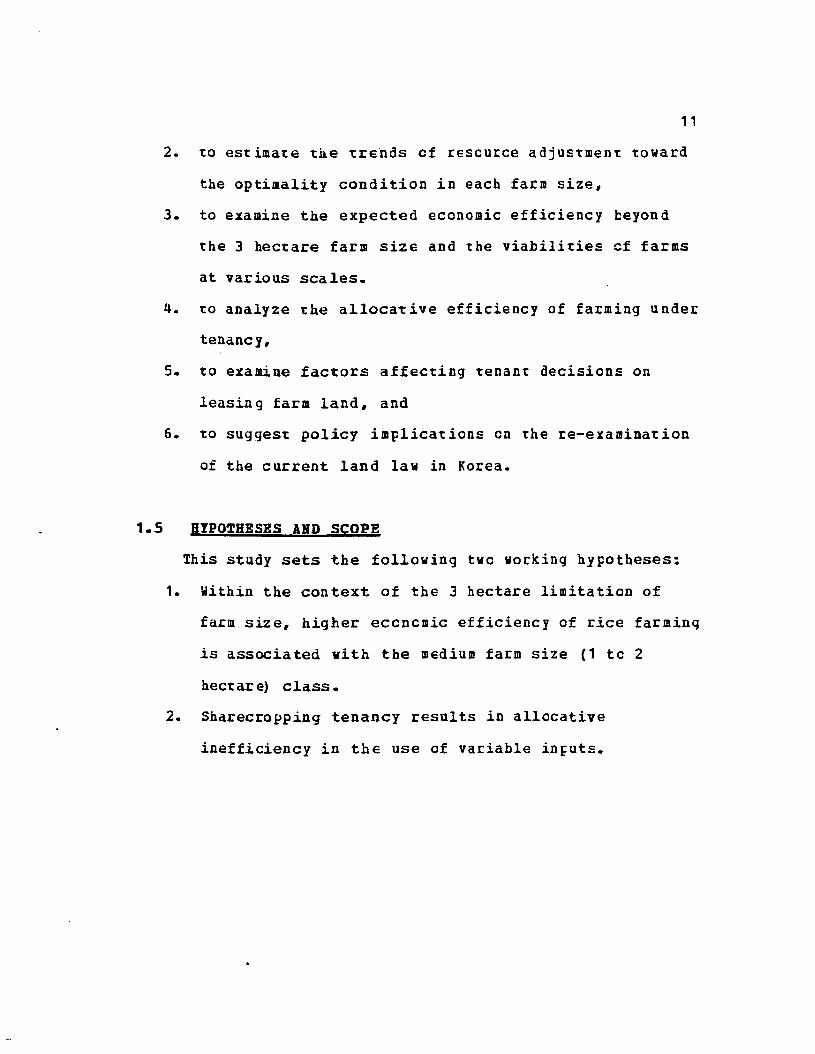
2. to estimate the trehds ef reseurce adjustment toward
the optimality condition in each farm size,
3. to examine the expected economic efficiency beyond
the 3 hectare farm size and the viabilities of farms
at various scales.
4. to analyze the alloca~ive efficiency of farming under
tenancy,
5. to examine fac~ors affecting tenant decisions on
leasing farm land, and
6. to suggest policy implications en the re-examination
of the current land law in Korea.
1.5 HYPOTHESES AIID SCOPE
This study sets the following two working hypotheses:
1. Within the context of the 3 hectare limitation of
farm size, higher econemic efficiency of rice farminq
is associated with the medium farm size (1 tc 2
hect ar e) class.
2. Sharecropping tenancy results in allocative
inefficiency in the use of variable in~uts.
12
1.5.1 Rationale for Hypotheses
traditionally rice farming in Korea has teen
characterized by labor in~eDsive ~ractices. However, the
recent trend of declining farm population necessitates farm
mechanization. Farm machines which are ado~ted in rice
farming include paver-tillers, power-sprayers,
power-threshers, etc., sincE ~he large machines like
tractors, combines, and rice-transplanters are not
economical for small farms. Scme imFortant farm opera~ions
such as rice transplanting and harvesting still rely on farm
labor. Peaks in labor shor~ages are reached at the periods
of rice transplanting and harvesting. In this respect, the
major determinants of economic efficiency of rice farming in
Korea would be the following: 1) the available labor supply
to effeCtively per£orm the labor intensive farm oFerations;
and (2) the availability of machinery adaptable to farms of
3 hectares or less. As farm size becomes smaller, the farm
operations are increasingly mcre labor intensive. On the
other hand, larger £ar~s may emFlcy a greater percentage of
capital inputs. Larger farms may often display increased
efficiency through the use of these inputs. However, on
smaller farms, where lator is generally more available, peak
period la~or shortages are relatively less severe than for
larger farms. It appears that efficiency in the use of
13
labor may override efficiencies resulting from increased use
of ca~i~al equipment adaptab~e to the current farming
scales. ~hus we may hypo~hesi2e. ~ha~ higher economic
efficiency of rice farming is associated with the medium
farm size under ~he curren~ farming s~~uc~ute.
An earlier study shows that sharecroppers represented
32 pe~cent of ~he ~o~al ~enan~ farmers surveyed in 1977 and
that the rate of sharecropping rent was, on the average, 35
percen~ of ~he rice produced in the leased land (Oh, pp.
51-53). Even ~hough ~he propor~ion of share ~enan~s and the
tenancy still comprises one ~hird of prevailing rental
arrangements.
A review of li~era~ure reveals ~ha~ the alloca~ive
efficiency of share tenancy de~ends on the market system.
Cheung (1969a) insists that an equilibrium under a
competitive market system viII lead to efficient resource
allocation of share tenants. However, in Korea, tenancy
practices have been legally prchibited since 1950. Thus
there has been no well defined rental market that could
systemize rental arrangements. Most forms ot rental
con~racts are not instituticnally frotected. The ren~al
market system in rural Korea does not seem to satisfy the
conditions required for a competitive marke~. Onder this
14
situation, it is hypothesized, a sharecroFFing tenancy will
result in allocative inefficiency relative to owner
cultivation.
1.5.2 Scope and Procedure
The concepts of relative economic efficiency and
economies-of-scale are adopted as tools in analyzing the
relationship between farm size and economic efficiency.
Since both methods are static, the factor adjustment
behavior of farms toward partial equilibrium over time is
also analyzed. In addition, the farming scale is further
examined with respect to the expected economic efficiency
and farm viabilities beyond the 3 hectare barrier.
Allocative efficiency is tested to see if tenant
farmers are utilizing variable inputs at optimum levels. In
addition, factors influencing the a~cuDt of land under
tenancy is investigated in the framework of demand and
supply sides in a rental market.
In the process of accomplishing these tasks, Chapter II
presents the institutional ~ackgrcund of Korea's current
land law. Chapter III contains a review of current
literature on the farm size and economic efficiency, and on
land tenure and allocative efficiency.
15
In Chapter IV, analytical models are explained which
will te used in ~he analysis. !hese lodel include the
profi t function for the analysis of economic efficiency, the
survivor technique and ~he sca~~er diagram ap~roach for ~he
analysis of economies-of-scale, and the distribu~ed lag
model for the analysis of the dynamic adjustment of resource
use ..
In Chapter V, the empirical findings are reported from
the analyses of rela~ive econc~ic efficiency by farm size,
the economies-of-scale, and the dynamic resource use
adjus~ment by farm size. In addition to the above analyse~,
the discussion is further opened up about the economic
efficiency associa~ed with farm size beyond the 3 hectare
limit ation..
Chapter VI analyzes allocative efficiency £y tenant
farmers and examines fac~ors de~ermining the size of ren~ed
land.
Finally, Chapter VII snmaarizes ~he research findings
and suggests policy implications with regard to possible
changes in farm s~ruc~ure..
Chapter II
INSTITUTIONAL BACKGBOURD OF tHE LARD tAW INKOBEl
2.1 IHTBODQCTIOR
7he underlying jus~ifica~ion for land reform in
developing coun~ries can be fcund in ~he following
statement:
In many peasan~ coun~ries of the old wcrld, theaverage landvorker operates cnly slightly abovethe subsis~ence level. His desire ~o shif~ to ahigher scale is frequently limited by custom, tyhis lack of capi~al and kncw-how,· by his rela~ive
inability to acquire additional land in his ho.ecommuni~y, and by ~he abse[ce of ~ublic policiesand programs for this purpose (Barlowe, p. 151).
In this respec~, land reform is cne of the s~rongest
measures used to direct publicly ccntrolled change in the
existing charac~er of land cwnership in countries where the
great majority of the peoplE are dependent upon agriculture
and where outmoded ~enure sys~ems have favored small classes
of landlords. This principle was applied in Korea when
land reform was enac~ed in 1950.
- 16 -
17
2.2 PRE-LAND BE.Poaa PEBIOD
Prior to land reform, the land tenure system in Korea
has been termed semi-feudal (or feudal in some cases). The
size of land holdings de~ermined ~he social ~osi~ion of ~he
landlord, and a traditional sutordinate relationship existed
be~ween landlords and ~enan~s. Moreover, ~he marked
characteristics of the land tenure system can 1::e depicted by
high ren~s and insecure ~enan~ righ~s. In addi~ion, Korea
was under the Japanese rule from 1910 to 1945. Thus the
land tenure system was closely rela~ed ~o JaFanese ruling
policies, such as Japanese landownership? and taxa~ion,
which secured the staple foods for Japan durinq iorld iar
II.
The scale of farm management was small. About 90
percent of farm households cul~ivated less ~han 2 hec~ares ,
and the tenanted land was 63 percent of the tctal cultivated
area (see Table 2.1). Under 1I0S~ t e aancy contracts, r enr s
were as high as 60 percen~ of ~he crop yield (Pak 1956, p.
1015). In addition, tenants themselves had to pay for
cos~ly fertilizers, farm il~lemen~s, seeds, and o~her
inputs. Along with these conditions, the semi-feudal
rela~ionship between landlords and tenants was reinforced
because landlords had the riqht to terminate leases at will.
7 About 62 percent of the landcwners holding more than 100hectares was Japanese in 1927 (Choi 1970, p. 352) •
TABLE 2.1
Changes in Household Distribution by Farm Size and Land AreaFarmed by Tenants - Before and After Land Reform in Korea
laborers, and (5) farmers who returned from abrcad. Farmers
who purchased land from the govern~ent had to pay 150
percent of the average output. The payment was supposed to
be made in kind and be finished in 5 years in terms of equal
annual payments.
Ey 1957, a total of 470,022 hectares was distributed.
Fifty seven percent of this total was purchased by the
government and the remaining 43 percent was confiscated land
22
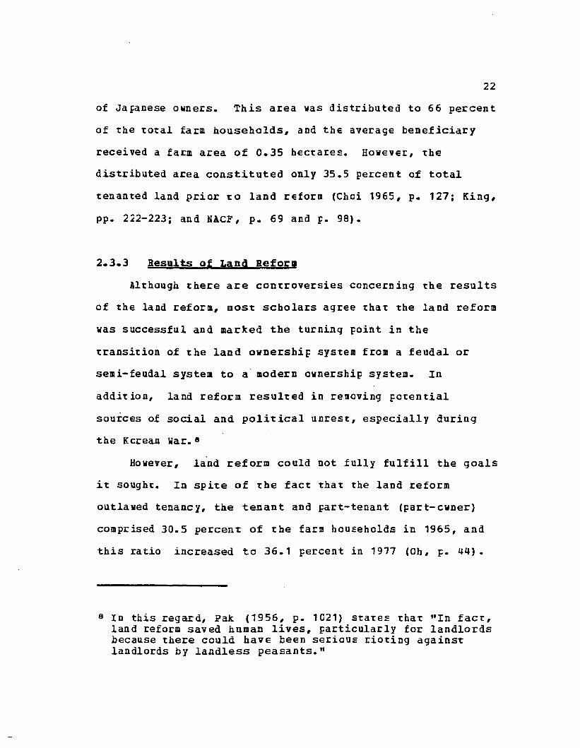
of Jafanese owners. This area was distributed to 66 percent
of the total farm households, and the average beneficiary
received a farm area of 0.35 hectares. However, the
distributed area constituted only 35.5 percent of total
tenanted land prior to land reform (Chci 1965, p. 127; King,
pp. 222-223; and NACF, p. 69 and p. 98).
2.3.3 Results of Land Refor,
Although there are controversies concerning the results
of the land reform, most scholars agree that the land reform
was successful and marked the turning point in the
transition of the land ownership sYStem froll a feudal or
semi-feudal system to a" modern ownership system. in
addition, land reform resulted in reloving potential
sources of social and political unrest, especially during
the Kcrea.n War. 8
However, land reform could not fully fulfill the goals
it sought. In spite of the fact that the land reform
outlawed tenancy, the tenant and part-tenan~ (part-cwner)
comprised 30.5 percent of the farm households in 1965, and
this ratio increased to 36.1 percent in 1977 (Oh, p. 44).
8 In this regard, Pak (1956, p , 1021) states that "In fact,land reform saved human lives, particularly for landlordsbecause there could have been serious rioting againstlandlords by landless peasants."
23
ihis trend was ca~sed, in Ea~t, by the fac~ that
beneficiary farmers of land refcrm often could no~ keep
purchased land after the payment period. This resulted
prima~ily from a lack of capital to operate farm. Survival
in farming was affected by the following conditions: (1) The
short repayment period (5 years), (2) the high monetary
interest (24 percent per anr.um), and (3) the stipulation of
repayment in kind. After the land reform, administrative
defects were found in the lack of institutional supports,
such as credit facilities and extensicn services. As
Ledesma (~. 37) notes:
••• even though patterned after the Jafanesemodel, the Korean experience did not fare as well••• for lack of government auxiliary services •••
Such adverse conditions often forced the farmer to illegally
sell part of his land even before the legal repayment period
ended, giving rise to a new breed cf tenant farmers.
In addition, political considerations affected the
legislative process. At first, many conservative
politicians and landlords resisted land reform cODcepts.
But as some sort of land reform became inevitable, landlords
began to sell their lands under conditicns favorable to them
Defore the reform could be implemented. By the time land
reform was enforced, the area cf land affected had been
drastically reduced. The inadequate and inefficieDt
24
administration of ~he ~ime cffered ~mple oPfCrtunity for
landlords to reyis~er ~heir lands under various disguised
forms of ownership. The absence of land reform to apply to
forest land and orchard land also permit~ed landlords to
preserve their landed properties to some extent. Moreover,
the outbreak of ~he Korean War in 1950 retarded the
enforcement of legislation. As d conseguence, by the year
1957, the redistributed area vas cnly 35.5 percent of the
to~al ~enanted area and only 45.9 percent of the area ~hat
the government initially planned for redistribution (Choi
1958, p. 127).9
9 According to Oh (p. 15), as of 1961, the Iedis~ribu~ed
area was 37 percent of the total tenanted land and was63.7 percen~ of the ~arge~ed area.
Chapter III
REVIEW OP LITEBATOBE
~his chap~er reviews ~he ~elevant literature on the
proDlems of farm size and land tenure in relaticn tc
economic efficiency. The review covers ~he theories and
methodologies used in analyzing economies-of-scale and
relative economic efficiency. Fo~ the land tenure ~roblem,
consideration is given to lite~ature on allocative
efficiency. Li~erature reviewed in this contex~ involves
theories concerning the effect of tenure 'systems,
par~icularly sharecropping ~enure, on the use of variable
inputs.
3.1 PABa SIZE ABD ECOR08Ie EFPICIERCY
Farm size has long been an important issue in
agricultural economics. While the issue deserves
substantial attention for a numter of reasons,10
'efficiency' has been an analy~ical focus in Froduction
10 Stanton (p. 727) summarizes an im~ortant mixture of thereasons: 1)poverty in rural area and ainimum level ofliving for farm people, 2) business management ofindividual farm, 3) efficiency, and 4) distribution ofag~icultural resources.
- 25 -
26
economics. With the conce~~ cf efficiency, we may consider
the least cost use of a given bundle of resources for
individual farm units and, also, across whole groups of
farms.
7here are basically twc concepts for the analysis of
efficiency and farm size: economies-of-scale and rela~ive
economic efficiency. The two are net mutually exclusive
for the purpose of farm size analysis. The conce~~ of
economies-of-scale helps to determine the best advantages in
produc~ion when a firm adjus~s scale or size. On ~he
other hand, the relative efficiency concept enables one to
compare levels OL economic efficiency between differen~
firms, or firm size groups. While the economies-of-scale
concept theoretically compares the mcst efficient firm in
each scale or size, the relative economic efficiency concept
may nc~ always include ~he Dost efficien~ oFera~ion in each
scale or size.
3.1.1 Economies-of-Scale
Where the relationship between farm size and economic
efficiency is concerned, Jacob Viner's long-run cost curve
has been widely accepted. ~he lcng-run average cost curve
or the economies-of-scale curve is given as an envelope
curve which is tangent to the family of shor~-run average
27
cost curves. Any point on the economies-of-scale curve
shows the least-cost combination cf inputs required to
produce a specified ou~pu~. Generally we assume aU-shaped
long-run average cost curve. The declining part of the long
run average cost curve proves economies of scale, whereas
the rising part of it determines diseconomies of scale. The
long-run average COSt curve or the economies-of-scale curve
is also termed the long-run planning curve, because i~ shows
the cost advantages, or disadvantages, for Ferspective firms
of various sizes (Bressler 1945; Carter and Dean).
~be empirical analysis of economies-of-scale can be
ca~egorized into three groups, according to tbe data used
which determine ~be me~hod, the scope, and the
inter~retation of the result: 1) analysis using Census data,
2) analysis using sampled cross section data, and 3)
analysis using synthesized data.
Census data are sometimes used tc show trends in the
size distribution of firms and to piDpoiD~ the most
efficient firm size. This approach was originated by
Stigler (1958) and is termed the Survivor Technique. This
method assumes that, in the long-run, firm sizes ~hich are
efficient will survive and firm sizes which are inefficient
will decline. Firms in Lhe size class which show an
increase in their relative outfut share in the industry are
28
presumed to be o~timal. The survivor ~echnigue is appealing
because it ~ simple and avoids statis~ical problems which
might appear in cross-section analysis (Lund and Hill;
Stanten). This method is sUPEerted by evidence of its
usefulness in determining opt imal scales, and in predict ing
impending cha nces in an ind USt ry (Saving; Weiss; Pasour).
However, the survivor technique may not provide a valid
indicator of the economies-of-scale because firms may
survive for many reasons other than their internal
efficiency (Bain). French suggests that environmental
condi~ions pertaining to the extent ef the ~a[ket and the
sources of raw materials are other factors which affect the
firm's survival. Xn addition, since the prefit-maximizing
size may not, under the real life conditions, he at the
lowest point of the long rur. average cost curve, one may
expect fiLm operations to adjust toward sizes well teyond
the most efficient size on the economies-of-scale curve
(Lund and Hil~; Badden and Partenheimer).
!he average regression analysis has been widely used
for samfled cross-section data. ihis approach has the
advantage of estimating production and cost functions and
testing theoretical hypotheses abeut ~hem. However, even if
~e assume that there are no statistical problems such as
sampling, aggregation, specification, and measuremen~,
29
regression analysis of economies-of-scale has several
shor~comings. The regression line is an average or central
~endency line which does no~ necessarily con~ain the ~angen~
points with the envelope. As a least-squares reg~ession is
fit~ed to ~he cross-sec~ion da~a, the result is a curve ~ha~
goes somewhere through the middle of the observed pcints
(Walters). In addition, Bressler (1945, F. 528) s~a~es
that:
Unfortunately, it combines and confuses cos~
changes that result frcm the more completeutilization of a plan~ of a given scale with thecost changes that accompany in scale.
This is because sampled fa~ms may be operating with
non-optimum resource combinaticns. A related ty?e cf
difficulty in the reqressio~ aFFroach is referred to as the
regression fallacy (stigler 1952). Jchnson (196Q, p , 184)
describes this:
••• the regression fallacy is alleged to entercross-sect ion co ae studies by r ra nsd tionaldisplacements in output with a disproportionatechange in accounting coSts so that an extremeobservation of high output viII show an unusuallylow per unit cost and conversely fer an extremelylow output observation. .
Accordingly, the average line obtained from regression
analysis is highly suspect and cannot te regarded as an
estimate of the theoretical ecctomies-of-scale curve.
Some attempts have teen made to avoid the problem of
regression fallacy. One attemI:t is to incorporate a measure
30
of capacity as a variable in the statis~ica1 analysis
(Carter and Dean; Philli~s). In this case, th~ capacity
measure is commonly used as a shift variahle. When this
variable is set at 100, or full capacity, the estimated
curve should correspond to the usual concept of the
economies-of-scale curve, i.e., ~he envelope curve. The
main problem with this analysis is the definition of
capachy. A measured capacity may represent a bottleneck of
some item of equipment, rather than a real capacity of the
firll. E'"en without this difficUlty, we may e xpece a joint:
relationship bet~een costs and capacity and scale (Bressler
1945) •
Another attempt is the estimation of the covariance
cost funCtion, combining both time-series and cross-section
data (Johnson 196~). This approach may have an advantage of
providing a test for the existence of the regression
fallacy. It has also been argued tha~ the covariance
analysis reduces the risk of simultaneous eguation kias in
estimating the production ox cost function (Bach). While
the covariance analysis can avoid the regression fallacy, it
may produce a peculiar hybrid type of function that is
difficult to interpre~ (French). Therefore, we have to note
that each of the attempts explained still produces an
average regression, but the things averaged may differ.
31
AI~erna~ively, Bressler (1945) has sugges~ed ~ba~
instead of fitting regression functions, the long-run cost
func~ion might be estimated as an envelope curve to the
bo~~om of ~he cos~-volume scatter diagram when only
cross-section datd are avialakle. Bressler (1945, p.529)
insists tha~:
••• it represents an attempt to define the locusof the lowes~ cos~s ~ha~ were obtained a~ variousvolumes, and as such will approach the economy ofscale curve in so far as ~he ac~ual sample ofplants included some which were efficientlyorganized and opera~ed ~o ca~aci~y. .
Thus the true envelope or the long-run average cost curve
would more nearly correspond to ~he bo~tom edge of ~he
scatter diagram (Madden and partenheimer). ihen we use this
approach, however, we need enough observa~ions to include
wide Ianges of volumes, especially in large scale. Although
a few studies applied this ap~roach,11 it has received
considerable a~~en~ion wi~h respect to the ~roducticn
function. This is related to the so-called 'Frontier
Produc~ion Function' which will be explained in detail when
we di$Cuss the relative economic efficiency.
As an alternative to ~he methcds ~reviously discussed,
the economic-engineerinq approach utilizes synthesized data
to estimate COSt functions. Engineering, biological, or
other detailed speciiicaticrs cf input-outpUt relationships
11 One example of this approach is seen in Ct~oson and Epp.
32
are synthesized to develop short-run average cost curves,
which in turn construct an envelope curve. This approach
was initially suggested by Bressler (1945). 1he empirical
application of this approach has mostly been conducted in
experimental research stations (For example, Chan, Eeady,
and Sonka; Johnston 1971; Matulich, Carmen, and Carter;
Moore).
The economic-engineering approach avoids many cf the
problems encountered in statistical approaches. One may
apply it to cases where acccunting record data are not
available. Once the basic information on the engineering,
biological, or other input-outpUt relationships has been
obtained in one area, it can be useful in others. likewise,
as technical relationships, or technologies, change in some
of the operations, it is relatively easy to utilize these
changes in the total farm operations in order to determine
the effects of these changes on the si2e or scale. In
addition, the economic-engineering approach suggests what is
possible in the farming operation, while statistical
analysis using sampled data indicates what is being done
(Faris; Faris and Armstrong).
The major limitation of the Economic-engineering
approach is that it reguires high research cost. The
technical details required to synthesize a COSt function are
33
the main source of the higb ex~enses. This approach also
tends to omit some aspect of short-run cost as the size and
complexity of the o~era~ion increases (Black). The
economic-engineering approach has been criticized in that it
is a kind of abs~ract analysis. This is because product and
factor prices are assumed constant and technical
coefficients are determined from selected sources such as
experimental data, progressive farm data, etc. The
economic-engineering approach has shewn few findings of
diseconomies of scale. This is attributable to the use of
constant input coefficients and the inability to measure or
account for coordination problems as firm scale increases.
ihen synthetic estimates are obtained, they need to be
checked against alternative sources of information,
particularly actua~ performance of firm operations (French).
Accordingly, the economic-engineering afproach without the
knowledge concerning the physical production functicn along
with the existing price re~aticnshifs may not pro~ide an
accurate synthesis of the cost function (Heady 1956; Olson).
So far, we have reviewed three general approaches for
the analysis of economies-of-scale. Each has its own
justification as well as limitations. However, the optimal
choice will depend on the objectives of the study and the
funds and data available.
34
3.1.2 Relative Economic Efficiency
Economic efficiency is the main concept which
economists use to analyze the rationale of farm decision
making. If farmers are inefficienct in their management of
resources, then agricultural production can be raised by
simply improving the alloca~ion of resources ~i~bou~ having
to develop new technology and absorbing additional resources
(Farrell; Lau and Yo~opoulos 1971; Pachico).
Economic efficiency has been used as a relative concept
since it is almost impossitle to set an absolute level of
economic efficiency (Hall and Winsten; Pasour and Bullock).
Economic efficiency can be split into technical efficiency
and alloca~ive (price) efficiency. 7ecbnical efficiency, as
an engineering concept, is entirely abstract from the effect
of price. Technical efficiency refers to whether firms
obtain the maximum amount of output given the inputs in
production. In ~erms of a relative efficiency, a firm is
said to be more technically efficient than ancther if it
consisten~ly produces greater output from the same
quantities of measurable inputs. Differences in technical
efficiency are essentially differences in management
factors, such as the technical knowledge, will, and effort.
The major sources of technical inefficiency are related to
technology, i.e., the complexity of technology and the rate
35
of change of the technology (Pachico). On the other hand,
allocative or price efficiency is a behavioral concept. A
firm is allocative-efficient if it maximizes profits by
equatinq the value of marginal Froduct of each variable
input to its opportunity cost. Allocative inefficiency thus
represents resource wastage.
~he measurement of economic efficiency is an important
problem for both the economic theorist and ~he econemic
policy maker. Several methedologies have been developed in
order to measure rela~ive econemic efficiency. Perhaps the
most common approach has been to compare the behavicr of the
best operating firms with the firms in guestion. Farrell
developed an isoquant which is an envelope curve of the
observations in the inputs and unit output space using
linear programming. In drawing an envelofe isoguant, ~here
is no restraint e%cept the shaFe of iseguant as a convex
curve ~o the origin. Since the isoguant reFresen~s the most
efficient performances among the observations, it is called
a 'frontier production functien'. this relationshiF can be
illustrated for the two-inputs, one-output case as seen in
Figure 3.1 •
!he unit isoguant UU' shows technical FOssibilities for
efficient production, and any Feint en this isoguant can be
termed technically efficient. In the Figure 3.1, fer
o
36
Figure 3.1: The Unit Isoquant and the Measurement ofTechnical, Allocative, and Economic Efficiency
37
instance, points band d represent the actual·processes
which are technically efficient. On the othe~ hand,
observation c is technically inefficient. Its technical
efficiency is defined as the ratio of tbe distance between
the o~igin to band tbe distance between the o~igin to c,
i.e., ob/oc. Points band c represent the same factor
proportions.
Allocative or price efficiency can be measured when
input price level appreas as a~ isoccst line. While points
band d in Figure 3~1 are technically efficient, only
observation d is allocative-efficient given the isocost line
PP'. Point d assures the minimum cost in producing a unit
of oUtpUt.. The alloca'tive efficiency of Foint c is
estimated by the ratio of the cost implied 1::y the l.owest
possible isocost line 'to 'the cOSt at point 1::, i.e., oa/ob.
Thus the measure of al.locative efficiency is determined as
tbe ra'tio of 'the minimum cost at the optimum factor
propo~tion 'to the minimum cost given the factcr p~oportion
observed.
An estimate of overall, or economic efficiency, is the
product of teChnical. efficiency and allocative efficiency.
Thus the economic efficiency of o1::servation cis:
(ob/oe) (oa/ob) = oayoc , 'Ibis is the ratio of minimum
production cost to actual observed cost.
38
Some problems are associated with Farrell's approach.
The most prominen~ problem may te the reliance cn ot~liers
for the computation of the unit isoquant. For this, Farrell
(pp. 260-261) s~a~es ~ha~:
••• price efficiency is very sensitive to theintroduction of new observations and to errors inestimating factor prices, so that i~ is likely tobe rather unstable.
ibile parrell has confidence in ~he measure of technical
7he difference in output tetween 'average' firmand the extreme positive outlier is used tomeasure the technical inefficiency of the averagefirm. Another in~erpre~a~ion, of course, couldhave the 'average' firm re~resentiDg the norm andthe positive ou~lier represen~ing an unusual .endowment of some fixed factor of production, suchas entrepreneursbip, or luck. It may representthe classical source of error in measurement or ofnoise in the universe, and as such it can im~ly
nothing systematic about efficiency.
An alternative approach ~o estimating relative economic
efficiency is a profit function model. This method depends
on the theoretical duali~y te~weeD ~he produc~ion func~ion
and profit function. Nelson regards the exploitation of
duality rela~ions as an importaD~ recent methodological
development in production function fitting. Be points out
the advantage of duality theory as it permits greater use
of price data in estimating production relations.
39
Lau and Yotopoulos (1971) fi~st applied the
Uni~-Ou tpu~-p rice «(JoP) profi ~ f unc t Lcn to aq r LcuLr ural
production. The pro£it function characteri2es a firm's
maximized profit as a function cf the price of output. the
prices of variable inpu~s. and guantities of the fixed
inputs. They maintain that the profit function analysis is
a method based on the precepts cf economic theory. and is
more general than the existing alternatives. 1 2 lau and
Yotopoulos (1971, p. 95) indicate ~he sho~tcomings of the
alternative approaches by stating:
The deficiencies of ~he exis~ing afP~oaches tomeasuring efficiency should dictate the minimum~eguirements tha~ a new ccncept of relativeeconomic efficiency should meet if it is to be atall useful. (i) I~ should account fOl firms thatproduce different quantities of output from agiven set of measured inputs of production. Thisis the component of differences in technicalefficiency. (ii) I ~ should take Lnr o accoun e thatdifferent firms succeed tc varying degrees inmaximizing profits, i.e., in eguating the value ofthe marginal product to each variable factor ofproduc~ion ~o i~s price. This is the component ofprice efficiency. (iii) The test should take intoaccoun~ that firms opera~e a~ different sets ofmarket prices.
12 The existing alternatives ccrpared are as follows:partial productivi.ty and total productivity indices foreconomic efficiency measuremenq index of marginalproduct and opportunity cost for allocative efficiencyestimation; and produc~ion function apFrcach andFarrell's frontier function aPFroach for technicalefficiency measurement.
40
7he profit function, hcwEver, requires gccd price data
for inputs and outpUts. The profi~ function approach will
provide a reasonable ~est of relativE econemic efficiency
only when this condition is met. Moreover, this methodology
permits only the examination of relative efficiency between
groups of firms.
3.1.3 EcoDoaies-of-scale in Relation to BelatiYe BcoDoaicEfficiency
Since every point on the long-run average cost curve
shows the optimal combination of inputs in each scale, the
economic efficiency of an observation eff the curve will be
aeasuxed relative to the point on the envelcpe curve. If
all observations lie on the economies-of-scale curve, then
this curve itself measures relative economic efficiency.
When some observations are not on the ecvelofe curve, the
economic efficiency of such an observation is determined as
follows. The observation viII te first compared with the
optimal point of th~ particular scale ot size. This is the
economic efficiency given scale (EES),13 i.e., a measure of
the relative cost of produc~icn given scale. Then, the
economic efficiency of the optimal point of the particular
scale will be compared with the lcwest point cf the
13 See Seitz for details OD the technical efficiency and theallocative efficiency in rela~ion with different scales.
41
economies-of-scale curve. This is the measu~emen~ of
economic scale efficiency (ESE), i.e., an overall measure of
the relative efficiency of alternative scale activities.
The economic efficiency of an ctservation will finally be
determined by the product of EES and ESE. Thus, the
economic efficiency is a measure of the COSt of produc~ion
of each observation relative to the lowest cost observation.
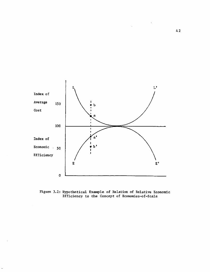
This ~elationship is illus~~ated in Figure 3.2
IL' curve in Figure 3.2 is an envelope cu~ve drawn in
terms of index of average cast, and EE' curve shows tbe
economic efficiency index of ~be envelcFe curve. The lowest
point of LL' curve, c, corres~onds to the highest economic
efficiency. The economic efficiency of observation b is
shown at point b', which is determined by the ratio of the
index of average cost at c and the index of the average cos~
at b.
The implica~ion of the relationshiF between the
concepts of economies-of-scale and relative economic
efficiency is that the economies-of-scale ccncept alone is
not enough to explain the relationship between firm size end
economic efficiency. While economies-of-scale shows the
optimal level of input combination in every scale or size,
relative economic efficiency cc~~a~es real Fhenomena of firm
operations on the average. Therefore £oth concepts are
42
L L'
150Average
100
Index of
Economic 50
Efficiency
E E'
a
Cost
Index of
Figure 3.2: Hypothetical Example of Relation of Relative EconomicEfficiency to the Concept of Economies-of-Scale
43
requi~ed to analyze economic efficiency with ~espect to
scale o~ size of firms.
3.2 111AHcr liD ALLOC1!IVE EPPICIEHCY
A debate on land tenure has long focused on the
relationship between tenancy, especially sharecropping
tenancy, dod allocative efficiency. A large numter of
economists maintain that sharecropping tenancy results in an
inefficient dllocation of resoorces (Adams and Bask; Bardhan
and Srinivasan 1971; Georgescu-Boegen; Ip and Stahl; Issawi;
Shickele). Others argue that the form cf land tenure has no
necessary bearing upon allocative efficiency (Bray; Cheung
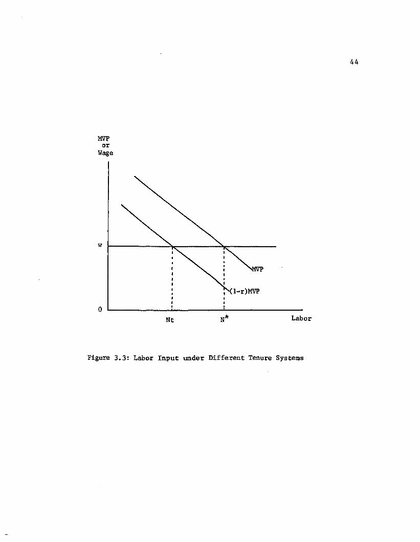
The inefficiency argument (or disincentive proposition)
is illustrated in Figure 3.3. In the figure, it is
assumed, for simplicity, that agriculture ope~ates in a
world of certainty, and that the cnly inputs are land and
labor. The disincentive argument is based on the fact that
the sharecropper's labor is utilized at Nt, where his
marginal return, (l-r)~VP, is equal to his alternative wage,
where r is the rate of share rental and MVP denotes the
marginal value product of labc~. On the other hand,
fi%ed-rent tenancy and owne~-fa~ming are regarded as
MVPor
Wage
w
oNt
(l-r)MVP
Labor
44
Figure 3.3: Labor Input under Different Tenure Systems
45
equivalent, since they utilize ~esources up to the foint
where marginal va~ue produc~ equals i~s OPFc~~uni~y cos~.
Thus, it is concluded that sharecropping leads to an
inefficient a~location of rEsourCES.
In contrast to the above argument, Cheung (1969a) has
argued tha~ sharecropping does not necEssarily lead ~o
allocative inefficiency. Cheunq's reasoning is that under
competi~ive condi~ions, priva~E con~rac~ing bEtWeen
landowner and tenant would lead to the same resource
allocation as if ~here had been ccmpeti~ive marke~s for
~abor and/or land~ This argument has been sU~Forted by Beid
(1976) and Roumasset (1978, 1979). In suppor e of Cheung's
proposition, Boumasset (1979) relies on a bargain~nq model
which involves viable contractual arrangements, undEr the
assumption that property rights are WEll-defined and
contracting costs are zero. Roumasset does not suggest the
possible outcomes o£ recontrac~ which make the recontracting
parties better-off, while Currie formulates theoretical
frameworks on the rearrangemen~ of ~he rental agreement,
which would lead the tenant to utili2e his resource at N*,
Figure 3.3 , and make both the landlord and the ~enan~
better-off. Examples of such a case, under the assumption
of cert aint y and cost less reCCD t r ac r i nq, are: (1)
recontracting with a fixed absolute rental paymen"t, (2)
46
recontracting for sharing ccsts as well as revenue, and (3)
recontracting with s~ipula~ed levels of tenant's Eesource
use under sharecropping. I. In this model, the bargaining
power of the landlord or tenant will determine the magnitude
of the gain obtained from the recontracting.
Although many recognize the importance of the
bargaining power of both parties in determining the rate of
rent and the allocative efficiency, little attention has
been paid to the source of bargaining power and its
relation to allocative efficiency under tenancy. Prom a
practical standpoint it is difficult to justify the
assum~tion of perfect competition and egual bargaining power
in the rental market. On this matter, Ip and Stahl (p. 21)
argue that:
Assuming perfect competi tien ipso facto impliesthat e~isting land tenure arrangements will teequally efficient. • •• In view of this, enewonders Why the debate has persisted along theselines.
This suggests that allocative efficiency is still a
problematical issue in land tenure, particularly in the
tenure systems in less developed countries where markets
vould be characterizd by imperfections.
14 Details are presented in Appendix c.
Chapter IV
ABALYTXCIL ftODELS
~his chapter contains explanation of the theoretical
and methodological frameworks fer analysis of relative
economic efficiency between farm groups, economies-of-scale,
and farm resource adjus~men~s over time.
The profit function can be used to test relative
economic efficiency which is subdivided into technical and
allocative efficiency. The survivor technigue and the
scatter diagram approach are introduced as methods for
investigating economies-of-scale. Finally the distributed
lag model is discussed in connEction with the farm input
~he profit func~ion mcdel has been widel} adopted for
efficiency analyses since Lau and Yoto~oulos (1971) used it
to analyze Indian agriculture. Using the Frofit function
model, we can analyze econo~ic efficiency in terms cf
technical efficiency and allocative or price efficiency.
The relationship of the ccnceFts of technical, allocative,
and economic efficiency are eXFlained below.
- 47 -
48
Assuming the produc~ioD functions for two firms are
given by:
(4.1) vI = Al F(~l , zl ) ;
v2 = A2
F(X2 , Z2 )
where superscrip~s identify firms, A is the technica1 term,
I indicates ~he vec~or of variable inputs, and Z the vector
of fi~ed inp~ts. If the twe firms are equally technically
efficient, then A1eg ua 1s A2• If they differ, thEn the
difference can be explained by differences in environmental
factors, in managerial ability, and in nonmEasurable fixed
factors of production.
the margina1 conditions fer ~rofit maximization are
given by:
aA1F(X1, ZI)= k 1 c1
(4.2) ax! j jJ
aA2F(X2, z2)= k? c? 1 k2>O
ax? J J k.>O, j=I, ••• ,mJ
J- j-- ,
where c j denotes an oppor~unity COSt of input j and kj is
an adjusting facto~ for equali~y between marginal product of
factor j and Cj_ 1£ a firm is perfectly successful in
equalizing the marginal product of input j to its price,
then xj assames value of one fer that s~ecific input. If,
and oo1y if, two firms are equally allccative-efficient with
respect to all variable inputs, then k3 = kI ' j=1, ••• ,m.
49
The null hypothesis of egnal relative economic efficiency
for firll 1 and 2 implies that Al = A2
and k~ = k~ ,
j=1, ••• ,II.the above relationships bet~een two firms can te
forllnla~ed in the profi~ function. With the ~roduction
function' = AF(X,Z), we may obtain a nominal profit, which
is defined as current total revenue less current total
variable costs,
m(4.3)
,P = p.AF(X,Z) - L
j=1c! X.
J J
where P' is profit, p is the unit price of output, and c~ isJ
the unit price of the j th variable inFUt. Dividing both
sides by p, ve get
(4.4) '11'
p'=-=
p AF(X,Z) -m
rj=l
c.X.J J
where '11' is defined as the "Unit-Output-Price" (UOP) profit
and c j = cj/P , which is defined as the normalized price of
the j th input. When the UCP profit is maximized by
satisfying the marginal conditions for variable inpUts, ~he
UOP profit is written as:
m
Ij=l
c.X~J J
50
By a well-kBown theorem proved by ~cPadden, the above UOP
profit func~ion can be expressed as (Iau and Yotopoulos
1911; Lau 1978) :15
*(4 .6) 1T = A G* (c/ A, z)
Thus, the actua~ UOP profit functions of the two firlls will
be
i=1,2.
On the basis of a priori ~heoretical contex~, the UOP profit
function is decreasing and convex in the normalized prices
of variable inputs and increasi~g in guan~ities of fixed
inputs.
In ~he expression of dual transformation, the derived
demand functions for variable inputs are given by the
Shephard-Ozawa-McFadden leama. The derived demand func~ion
is given by:
(4.8) , i=1,2; j=l, •• ,m.
The lemma also gives the supply function,
*15 For determining Xj , we use the marginal condition
a 1T = A aF(X,Z) = c. Then aF(X,Z) _ Cj
aXj
aXj J • aXj
- A .
This equation may ~e solved for the optimal quantities ofvariable inputs, Xj, as a function of the normalizedprice of ~he variable inputs and of the guan~ities of thefixed inputs: that is xj = fj (C/A, Z), j=1, ••• ,m.
51
i-1,2.
(Jsing egua'tions (4.8) and (4.9), we may I:ewI:i'te the (JOP
profit function as:
m i* ir O-ki) c~ aG*(4.10) TT
i =vi - L cix~ = J i:a1,2.A G + A a-r 'j-1 j J j.1 kj Cj
To the above equa~ion, we nov pI:oceed to specify 'the
appI:opI:iate fUDctiona~ form and formulate operational basis
for an empirical tes~ of rela'tive economic efficiency. A
Cobb-Douglas production func~icn with II variable inputs and
n fixed inputs is given by:
m a. m 13(4.11) V = A Lrr x.J ) (rr ZJ'q)
J=l J q=l
The corresponding (JO{) profit function is given by:16
-1 -1 -1
(4.12) /= A0- u) m -a· (1-~) n SqO-lJ)
(l-lJ) (j~1J ) ( q~1 )(c./a.) ZqJ J
wherem
u = 1: a· < 1.j=1 J
16 Befer to Lau (1978) for details about the derivation ofthe (JOP profit function frcm the pI:oducticn function.
By ditect computation using equations (4.8) and (4.10), the
actual UOP profit functioDs and the derived delland functions
are given in Eql1ations (4.14) and (4.15):
-1 -1(1-u) m m -et.j(1-u)
({Ai) (l - L et.j/kij») ( II (k~) )
j-1 j"1 J
-1 -1 -1m et.j (l-u) m -aj"(l-u) n 6q (l-u)
(jJ11(et.j) ) (jlh (ei) ) (q}h (Z~) )
i = 1, 2.
i= 1,2; j = l, ••• ,m.
Equations (4.14) and (4.15) can be written
* B*. . m • Ct.. n(4.14)' 1TJ. = Ai II (C7) J II (Z1) q
. j=l J q=1 q
a C•-.
53
vhere
1 -1-1(l-u) m . m -a. (l-u) m a. (l-U)
A; :: (Ai) (l - L eLj/k:) ( It (k~) J ) ( It (eL.)J )j=l J j=1 J j=1 J
'* -1a. - - a. (l-u)
J J
s'* q-1
S (l-lJ)q
mil( 1 - L a./k.) (1-~)
j=1 J J
From equation (4.14)', ve may ~heoretically compare ~he
economic efficiency of the tva firms. By vx:iting 11 and ~
for firm 1 and firm 2, respEc~ively, and taking ~he ratio of
constant terms, ve ha ve
~(4.16) -1 =
A;tIl
(1 - Ej=1
Se note that if Al = A2 and kj = kJ, then A1 = ~ and the
twO firms have iden~ical profit functions, which means that
the tva firms are eqaa11y ecoDcmic-efficien~.
54
the derived demand func~ions for variable iDFuts are
given by:
(4.17) j = 1, ••. ,me
!Sill ti pI yi.ng both sides of eguation (4.17) by * get- Cj.ln" , ve
* *CjXj aln 1T
(4.18) * = j = 1, .. ,m.1T aln Cj
For the Cobb-Douglas profit func~ion, it becomes
(4.19) *= a.J
j=I, •• ,m.
Applying this rela~ioDship and using the equations (4.14)'
and (4.15)', ve have
(4.20)i
1T
=. -1 -1
(k~) (k~) aj- *1aj
1=1,2; j=l, •• ,m.
From equa~ion (4.20), ve may ob~ain tva implica~ions for
. * *1 irelative efficiency tests: (1) 1.f a. = aj
, then k. = 1.0J J
and fir. i sa~sfies ~he marginal condition for profit
maximization i.n terms of utilizing input Xj. This is the
absolute allocative or price efficiency; and (2) if a~1=a~2J J
, then the two firms are equally allocative-efficient with
ceapece to the uae of Lnpue Xj • This is the criterion for
the tESt of relative alloca~ive efficiency.
55
7aking a natural logarithm to equation (4.14)' and
using equation (4.20), we get a Cobb-Douglas type actual UOP
profit func~ian model which is given by
i = 1, •••
(4.21)
(4.22)
mIn ~ = In A + Lai
i=l
ciXi ,--;-= a i , m.
where 1T deno~es ~he norllalized profit, C:i the normalized
price of variable input, and Zj ~he fixed inpu~ all in
physical unit.
70 compare relative econollic efficiency tetween tWO
groaps of farms, we may specify the OCP profit function
model as
m n(4.23) In ~ = In A + e D2 + L a. In c
i+ L B. 1 Z
i=1 ~ j=1 J n j
(4.24)Ci~
--=a1T i1
D1 + ai2
D2 i = 1, •.• ,m.
where Dk deno~es dumllY variable fer each farll group and aik
identifies each group's ai coefficient (k = 1, 2).
Es~illating the above equations join~ly, we can test the
following hypotheses:
1. Equal relative economic efficiency:
Ho: e = o.2. Equal relative allocative efficiency:
i=1 •••• ,m.
3. Equal technical and allccative efficiency.
56
This hypothesis is necessary because it is
possible for two farm groups to te equally
economic-efficien~ without being equally
technical-efficient or egually allocative-
efficient or Doth:
Ho: e = 0, ~il = ~i2 i = 1, ••• ,m.
4. Absolute allocative efficiency of each farm
group. This is to test whether each farm group
maximizes its profit:
Ho: Ct i = ~ik i = 1, ••• ,m; k = 1,2.
5. Constant re~urns to scale:n
Ho : La. = 1. o.j=l J
4.2 SOB'XVOB TBCHBIQUE ABn SC1T~EB DXAGBA! APPBOACH PORTHE ECOHOKIBS-Ol-SCALE lBIL1SIS
The empirical analysis of the economies-of-scale is not
an easy task to conduc~. In this s~udy, the existence of
economies or diseconomies of scale will be investigated by
the methods of the survivor Technique and the Scatter
Diagram. Since no single methcd is ccm~letely satisfactory
for analysis of economies-of-scale, these tWO approaches are
believed to provide more general evidence of eccnomies or
diseconomies of scale ~han any cne particular method.
57
4.2.1 The Survivor Technique
7he purpose of the survivor technique is to find the
optimal firm size class by examining the trend of changes in
number of firms in each size class o~ relative share of
output in the class over selected time inte~vals. If a firm
size class shows dn increasing trend in the relative
proportion in the number of fi~ls in an indus~ry over some
time intervals, then that firm size will be identified as
~he bESt surviving and, thus, defined as optimal.
The survivor technique is tased on Stigler's
proposition that the class of firm size surviving best would
have minimal average producticn COSts. Although the
survivor technique faces shortcomings, it is supported by
some evidences suggested in the previous chapter. The
survivor technique is a simple and indirect methcd of
determining economies of scale (Lund and Hill; Stanton).
The variables which will be considered in this study
include the relative distrituticn of farm numbers among
different farm size classes, and the average production cos~
per unit of output among different size classes.
58
ij.2.2 The Scatter Diagra. Aii~oach
The scatter diagram a~~roach, which was suggested by
Bressler (19ij5), will provide an envelope cu~ve along the
locus of the lowest points in a cost-volume scatter diagram.
Theoretically, the economies-of-scale curve ~~aces the
minimum cost of producinq each level of out~ut. Thus, the
envelope curve obtained from ~he scatte~ diag~am viII
closely represent the long-run average cost cu~ve. As
Stollsteimer, Bressler, and Boles argue, graFhic analysis
will give the researcher a "feeling" fo~ his data and
facilitat~ the use of the envelope or near-envelope curve
rathe~ than an average reg~ession line.
ij.3 DISTB~BOTED LAG BODEL
The necessary condi~ion fo~ the oftimal allocation of
the i th input will be met when marginal value product of
the input equals its price, i.e.,
a v pi(4.25) =
a Ii P
where V is production function, Xi is the i th input, pi is
the p~ice of the i th input, and P is the oU~fut price.
This constitutes a partial equilibrium. Multiplying both
sides of the above eyuation by Xi/V, we get
a v Xi pi Xi(ij.26) =
a Xi v P V
59
At equilibrium, the prodution elasticity of i th inFut
equals its factor share. ~hus, if it is assumed that
production is at equilibrium, then factor share can be used
as proxy value for production elasticity. However, the
assumption that econo~ic equilibrium is always attained is
dubious (Tyner and Tweeten 1965). We need, rather, the
alternative assumption that the employment cf a factor
(expenditur~ on the factor) tends to be adjusted towards an
equilibrium level. This suggests a distributed lag model as
defined below:
(4.27) F(t) - F(t-1) = A(E*(t) - F(t-l»
where E*(t) denotes the current equilikrium factor share, A
the proportion of adjustment tC the eguilib~ium made in one
time period, and F(t) the factor share of year t. Here the
character i identifying each input is dropped for a simpler
expression of the model.
Griliches has shown the basic raticnale cf an
adjustment model like equation (4.27). The Medel premises
that there exist some costs of adjustment such as: (1) the
cost cf being OUt of equilibrium; and (2) the adjstment
cost. If Doth types are quadratic, we can write the firm's
overall COSt function as2 2
(4.28) C(t) = a(F(t) - E*(t» + l:;(F(t) - F(t-l»
60
= 2a (F (t) - E* (t» + 2b (P (t) - F (t-1»(4.29)
where a is the unit cOSt of being CUt of equilib~ium, and b
is the unit cost of adjustment. 'Uie problem is to choose
F(t), given F(t-1) dnd E*(t), to minimize C(t). !hus,
a c ('t)
a F (e )
giving
(4.30) F (t) =a
d+bE* (t) +
bF(t-1)
a+t
aor F ('t) - F (t- 1) = (B* (t) - F (t-1) ) •
a+b
The adjustment coefficient, A , becomes a/(a+b). Only in
the case of zero adjus~ment cost(t=O), the A vould be 1.0.
As·the adjustmenc cos't 'tends to be higher, the rate of
adjustment would be slover.
Using the above model, we can ottain adjustment
coefficient and opcimal factor share. !heSE estimates will
be used to compare the resource adjustment Erocesses among
different farm size classes. the magnitude of the
adjustment coefficient indicates how flexible farmers are in
reallocating their resources tcwa~d new eguilibrium
condi tions.
Chapter V
PlRS SIZE lBD ECOBOSIC El'ICIEICY
In this chap~er we examine ~be rela~iensbip between
farm size and economic efficiency, and the dynamic
adjus~ments in resource use over time.
Economic efficiency of farm size classes is analyzed
using three methods -- the profit functicn medel, the
survivor technique, and the scatter diagram of unit cost and
OUtpUt. The profit func~ion medel is used to test
hypotheses of the relative economic efficiency among farm
size classes, while the survivor technigue and ~he scatter
diagram approach are employed te analyze the extent of
economies-of-scale. For ~he analysis of resource use
adjustment over time, a partial adjust_ent analysis is
carried OUt with a dis~ribu~ed lag model. In addi~ion, to
further evaluate the above analyses, an examination of the
expected economic efficiency level beyond the farm size
barrier, and the agricultural income levels at various farm
sizes, was conduc~ed.
- 61 -
62
5.1 RELATIVE ECOHOftIC EFFICIEBCY
lhis section discusses the estimation of the profic
function and the hypothesEs tests which are related to the
relative economic efficiency among differen~ farm size
classes. Farms are ranked intc four size classes according
to total cult.vated land area, as shown in ~able 5. 1, and
defined below.
5.1.1 Data and Par. Size Definition
Data used for this analysis were drawn from a 1977
cross-section farm survey of rice production costs conducted
by the Korean Kinistry of Agriculture 6 Fisheries. The
original data were collected ty the daily legs, in which the
farmer of the selected farms recorded every day's management
ac~ivity. A cotal 3,375 farms were selected for this
survey.
From the original data, farms in which rice ~rcduc~ion
yas the main productive activity or major income source were
identified. Thus, farms were selec~ed if their paddy land
area was greater than 50 percent of the total cultivated
land, and if ~he value of rice produced vas larger ~han 50
percent of the value of total farm output. In addition,
only cwner-opera~ors were considered for this analysis of
relative economic efficiency. ~his was done ~o elimiDa~e
63
the possible influence of the tenancy system when comparing
economic efficiency among different farm size classes. 1 7 A
total of 933 farms were selected for the estimation of the
UOP profit function.
Farm size can be measured in several vays. In this
study, farm size was measurd by the entire land area
operated by d farm. This method has teen widely used in
Korea; and agricul~ural s~atis~ics are pUblished using this
definition when they are separated according to farm size.
Four farm size classifications were outlined.
a) Small farms: farms cultivating less than 1 hectare of
farm land.
~ Kedium farms: farms cultivating 1and area from 1
hectare to 2 hectares.
c) Large farms: farms cul~ivating land area frail 2
hectares to 3 hecl:ares.
d) Extra-large far liS: farms CUltivating more than 3
hectares of farm land.
17 We will analyze the allocal:ive efficiency oftenant-operated farms in the next chapter.
5.1.2
TABLE 5.1
selected Owner-Farms by Farm Size
Farll Size Number ofFarms
Less thah 1 ha 530 56.8
1 - 2 ha 306 32.8
2 - 3 ha 67 7.2
Over 3 ha 30 3.2
Total 933 100.0
!odel Specification
64
the equa~ions es~ima~iDg ~be OOP profit func~ion and
the variable inpu~ demand func~ion are specified below:
(5.1) In ~ = In A + e2 d2 + e3 d3 + e4 d4
+ a In w + 8 1 In L + 82 In FN + 8 3 In K
w.HN(5.2) - = a 1 d1 + a 2 d2 + a 3 d3 + a 4 d4
~
where 'IT = UOP profit in Korean Won. Ncmina 1 ~rofi t
is calculated by SUbtracting hired waqe
bill from ~o~al revenue. ~heD the OOP
profit is obtained ty dividinq the nominal
6S
profi1: by u n.Lc-e o uc put J;:rice. 1 8
d1 = dummy variable: 1 for small farms;
0 otherwise.
d2 = dummy variable: 1 for mediull farms;
0 otherwise.
d3 = dummy varia.ble: 1 for large farms;
0 otherwise.
d4 = dummy variable: 1 fer eX1:ra-large farms;
0 otherwise.
v = the hourly wage ra1:e of hired label: (man-
equivalent) divided ly unit-output price.
L = 1:he physical paddy lard uni1:s measured as pyung. 1 9
FH = the ~an-eguivaleD1: family labor in~u~ in hours.
K = the imputed capital interests in Rorean Wen
for 'the fixed and flow ca~ital used in
producing rice.
HN = the man-equivalen1: hired labor input in hours.
In this analysis. hired lalor is regarded as a variable
input. Many oe he r ae ud Les have ~l:eal:ed family labor as a
variable input. However, the case of Korean family farms
seems different because of the serieus labor shorl:aqes in
18 The unit-output-price is ot1:ained by dividing totalre~enue by total physical output. 1he unit-output-priceis measured in Korean Won J;:€r kilegram ef froduced rice.
19 A 3,000 pyung is almost: equ Lva Ie ne to 1 hec t a r e which isabcut 2.5 acres.
66
rural areas. Family labor should be fully utilized
regardless of its opportunity cost. This wculd be
particularly applicable as long as farmers try to maximize
short-run profits. Labor supplied above the family labor
contribu~ion, hired labor, can be regarded as a variable
input. Thus, labor is divided into hired labor as a
variable input and family labor as a fixed inFUt.
In the above profit function, wage rate is specified as
a price variable for hired labor. There are ether variable
inputs such as fertilizers and pesticides. However, their
prices are not specified as price variables in the profit
function because the prices of fer~ilizers and other
chemicals are mostly controlled by government and uniform to
every farm in Korea. ThUS, these variables are indirec~ly
included in capital variable, K. Fixed inputs specified
include land, capital, and faKily laeor.
5.1.3 BstiAatioa aad Hypotheses Test
the estimating equation (5.1) includes different
intercepts for each farm size class. Slopes for each farm
size class are assumed to be equal. This means the four
farm size classes have the sa~e profit function except for
the constant terms. Prior to estimating this equation, a
hypothesis of egual slopes of the profit function should be
67
tested for the different farm size classes. If the null
hypOthesis of egual slope cannot te rejected, an estimate"of
the UCP profit function can be made based on equation (5.1).
However, rejection of the null hypothesis requires separate
specification of equations for each farm class. Direct
comparison c: economic efficiency between farm size classes
is not possible with the equations estimated separately.
This hypothesis was tested by covariance analysis. 2 o The
computed i-StatiStic from the covariance analysis was 1.16
with (22,913) degrees of freedom, which is less than a
critical F-value at the five percent of significance level,
i.e., F(22,913) = 1.52. ~hus. the null hypothesis of equal
slopes for every fara size class cannot be rejected.
7he analysis indicates that the four farm size classes
have the same profit function except for intercepts, which
also means that they have the same Froduction function
20 FOL the test of the hypothesis, we first estimate cropprofit function separately for each farm size class. Letthe residual sum of squares of each eguation be rCi) 'rei), i=1,2,3,4. Then we calculater rr = r(1)'r(1) + r(2)'r(2) + r(3)'r(3) + r(4)'r(4).
Next we pool the data and estimate a UCP profit functionwith different intercepts using dummy variables. In thiscase, slopes are restricted to be the same for everyclass. Let e'e be the residual sum of squares of thepooled equation. Then we calculate the F-statistic fortestinq the hypothesis of equal slc~es: i.e.,
F = ((e'e - r'r)/(pk - P - k + 1»/{r'r/(D - pk», wherep = number of classes, k = Dumter of independentvariables including interce~t, and n = totalobservations.
68
except for technical efficiency terms. However, this does
not mean that they have equal allocative efficiency.
Allocative efficiency will be determined by ~he join~
estimation of the UOP profit function and the factor demand
function. Equation (5.1) and equation (5.2) were estimated
jointly using Zellner's seemingly unrelated regression
method (Zellner).21 The result of the estimation is given in
Table 5.2 •
In general, the signs of the estimated coefficients are
consistent with ~he theore~ical ~ro~erties cf the profi~
function, except the coefficient for family lahore It seems
that the negative sign for the family labor comes from the
process of joint estimation of the profit func~ion and the
hired labor demand function. When the profit function is
estimated by the ordinary leas~ sguares method, the
parameter of the family labor is positive and significant.
Due to the correla~ion across models, the parameter turns
out to be negative while the tvo models are being
systematically estimated by the seemingly unrelated
regression method. However, it is unlikely ~hat ~he
parameter for family labor influences the hypctheses tests
of relative economic efficiency. The coefficient of family
labor is negative, but statistically insignificant. The
21 Seemingly unrelated equaticn mcdel is cODcef~ually
eX~lained in Appendix B.
TABLE 5.2
Joint Estimation of UOP Profit Function and Factor DemandFunction for Owner Farmers in Rice Production, 1977
(4) a 1 = a 2 0.06(1,1854) Maintained(5) a 1 = a 3 7.29(1,1854) Rejected at 5%(6) a 1 = a 4 6.28(1,1854) Rejected at 5%(7) a 2 = a 3 7.45(1,1854) Rejected at 5%(8) a 2 = a 4 6.51 (1,1854) Rejected at 5%(9) a 3 = a 4 0.30(1,1854) Maintained
III. Equal Relative Technical and Allocative Efficiency
(10) e3 = 0,
a 1 = a 33.89(2,1854) Rejected at 5%
(11) e4 = 0,a 1 = a 4 3.18(2,1854) Rejected at 5%
IV. Absolute Allocative Efficiency
(12) a 1 = a 0.03(1,1854) Maintained(13) a 2 = a 0.05(1,1854) Maintained(14) a 3 = a 0.15(1,1854) Maintained(15) a 4 = a 0.33(1,1854) Maintained
similarity of resource allocation between different farm
size classes. Whe~her thei~ resou~ces are al1oca~ed a~
optimum levels is not a matter of concern in this test.
Even though tWO farm classes de nct OFtimally utilize
variable resources, allocative efficiencies may appear
egual.
!he hypotheses tests show that small farms and medium
farms have equal relative allcca~ive efficiency, and ~hat
larqe farms and extra-large farms also have equal relative
allocative efficiency. BU~, the small and medium farms, as
74
a group, and the large and extra-large farms, as anether
group, are significantly different in relative allocative
efficiency. This resul~ does no~, however, indica~e whe~her
or not each farm size class utilizes hired lator at the
op~imum level for profi~ maximization.
5.1.3.3 Joint Test of Equal Belative Technical andl~ocatiYe Efficiency
ihen tVO farm classes shew equal relative economic
efficiency, a joint hypothesis of egual relative technical
and allocative efficiency mus~ he tested. EVED though ~vo
farm classes are equally econemic-efficient, they may differ
in ~echnical efficiency, allocative efficiency, ox to~h.
In this study, large farms and extra-large farms
appear to be equally as economically efficient as small
farms. The join~ hypo~hesis, hcwever, does not seem
necessary because differences have been shcVD in the
allocative efficiency between siall fa~ms and large farms,
and betveen small farms and extra-large farms. As expected,
the joint hypo~heses are rejected at the five percent level
of significance. This implies that differences in technical
efficiency compensate for differences in allocative
efficiency to result in equal relative ecoDomic efficiency.
5.1.3.4 Absolute Allocative Efficiency Test
75
!he test of absolute allocative efficiency hypcthesis
in this study is to check if fa~ms in each size class equate
marginal value product of hired labor tc op~o~tunity cost
measured in terms of wage rate. ~he null hypotheses are not
rejected at the five percent significance level in all
classes. These results may ccnflict with the ~esults of
the relative allocative efficiEncy tests. From these
results, we may infer ~hat large and extra-Ia~ge farms
diffe~ relatively in allocating their hired labor f~om small
farms, but their allocaticn of hi~ed labo~ is not
significantly different from the optimal condition for
profit maximization. Moreover, if we give more weight to
the results of the absolute allocative efficiency test than
to the results of the relative allocative efficiency test,
we cannot conclude that thE fou~ farm size classes are
different in allocative efficiEncy with res~ect to hired
labor input. 2 2
22 Note that the ultimate critErion on allocative efficiencyis set by the profi~ maximization condition which is aninitiating point in deriving a dual relaticn of profitfunction from production function.
5.1.3.5 Constant Returns to Scale Test
76
the null hypo~hesis of cons~an~ retucns to scale is no~
rejected at the five percent level of significance. This
resul~ leaves open ~he possibili~y ~hat cons~aD~ ~e~urns to
scale may exist in Korean rice farming. However, drawing a
firm conclusion about ~he nature cf scale economies in
Korean rice farming is not advisatle at this Fcint and
further investigation follows. OU~ statistical analysis
thus far still does not pcovide sufficient evidence of the
real nature of scale econoDies. 2 3
5.1.4 Su••ary
Eased on the joint estimation of the ncp profit
function and the hired labor demand function, we were able
to tes~ hypotheses on ~he reiative economic efficiencies of
the four farm size classes considered in this study. The
results of the tes~s indicate that, in 1977, medium sized
farms cultivating between 1 to 2 hec~ares were economically
more efficient than other farms in producing rice. Compared
with small farms, the higher econcmic efficiency of medium
farms was due to a higher technical efficiency by default
since the hypo~hesis of equal relative allccative efficiency
23 As discussed in the review of iiterature chapter, this isrelated to the argument cn the disadvantage of usingregression analysis in estima~ing a long-run average cos~
curve.
77
be~ween ~he two farm classes was JaiDtained. Large and
extra-large farms appeared to be equally as economically
efficient as small farms. All farm classes showed that they
were able ~o satisfy the necessary ma~ginal conditicn for
profit maximization with respect to the use of hired labor.
A statis~ical hypo~hesis tes~ maintained cons~ant re~urns ~o
scale in Korean rice farming. However, no conclusion can be
drawn about the nature of scale economies. The issue viII
be fu~ther in vestiqated in the following sections.
5.2 ECOHOftIES-OP-SCALE
In this section, economies, and diseconomies, of scale
are examined with the scatter diagram a~proach and the
survivor ~echnique. These ~vc methods are sim~le in
application, but they can provide additional evidence on the
ac~ual extent, if any, of scale economies. If ~he resul~s
from these analyses are consistent and compatible with that
of the profit function analysis, then the relationship
between farm size and economic efficiency in Korean rice
farming would be more clearly unders~ood.
5.2.1
78
Scatter Diagram lpFcoach
The intent of drawing an envelope curve from a scat~er
diagram of unit cost and output volume is to find the lowest
possible unit cOSts at varicus OUt~Ut scales. the in~en~ is
to fit the bottom edge of the cost-volume scatter diagram to
a 'fron~ier' long-run average cos~ curve.
this approach was applied to the 933 sample farms which
were used in ~he profi~ func~ion analysis. In ~he sca~ter
diagram, the vertical axis shows unit production cos~ per
kilogram of rice and the horizontal axis shows volume of
produced rice in kilograms. !he unit production cos~s
include variable and fixed cos~s, taxes and fees, and
imputed cos~s of land, capi~al, and family labor. the value
of by-products is sUbtracted from total production costs.
Prom ~he diagram, the lowest points at various levels
of oUtpUt are drawn for each farm size. Figure 5.1 presents
the 'frontier' average cost curve by farm size. 2 4 ACl shows
the average cost curve for small farms; AC2 the average
cost curve for medium farms; Ac3 for large farms; and AC4
for extra-large farms. FrOD the-Figure 5.1, we can see that
the AC2 curve con~ains ~he low€s~ average cost among the
four unit cost curves. But it is not considerably lower
than ~he ACl curve. The average COSt curve for large farms,
24 The original cost-output scatter diagram is given inAp~endix Figure D.1.
Cost/kg (Won)
AClAC2
•
AC4
•
Output (kg)
Figure 5.1: The Lowest Cost Points at Various Output Levels by Farm Sizein Rice Production
....,\0
80
AC3, shifts up over AC1 and AC2. If we const~uct a long-run
ave~age cost curve with AC1, AC2, and AC3, which is within
permitted land size under current land law, the three curves
make a nearly U-sbaped long-ruD average cost curve. This
suggests an optimum scale within medium sized farms. The
lowest: possible uni't COSt is assumed to determine the
optimum scale. This is consistent with the results of the
relative economic efficiency analysis performed with the
profit function model.
Now consider the average cost curve for extra-large
farms, AC4. The lowest poin't on AC4 is lower than that on
AC3. This leads to an interesting implication in connection
with the legal limitation of 3 hectare land size. ACl and
AC2 de not significantly differ in their lo~est poin'ts.
However, the unit costs for farms between 2 tc 3 hectares
appear much higher rela'tive to the smaller farm size
classes. Further the cost curve for farms over the 3
hectare limitation, AC4, falls to a lover level than AC3.
This implies that within the limitation of the 3 hec'tare
ceiling, farming technology is confined to traditional
operations which are typically lacer-intensive. iith this
type of technology, the long-run average cost curve cannot
continue to descend as farm size gets cigger. Thus the
long-run average cost curve becomes a O-shaped one iithin
81
the 3 hectare farm size. In ccntrast, the extra-large
farms, for wha~ever reasons they may be cultivatinq more
land than legally permi~~ed, can adopt labor-saving large
farm machinery and equipment in order to reduce production
cos~ in the face of rapidly iDcIeasing wage ra~es in rural
areas. 2 5 When AC4 is included, the long-run average cost
curve no longer appears as a U-shaped curve. Ba~her, i~
resembles a V-shaped one. when one is determined ~o
integrate all short-run average cost curves into a a-shaped
envelope curve, one mus~ a~ leas~ assume tha~ the
alternative technological processes, which can be used at
different levels of ou~pu~, beccme Frogressively more
efficient until a certain crucial point is reached, after
which they become less efficient (Malanos, F.255). However,
in the case of Korean agriculture, technological
alterna~ives are discon~inucus and have not been adopted in
each case in a manner which reveals the full range of
increasing and decreasing returns to scale. It is,
therefore, difficul~ ~o de~er.ine which farm size is op~imal
in Korean farming from this survey data. If we include only
AC3 and AC4 in drawing an envelope curve, a declining
long-run average cost curve can be expected. What we can
conclude from ~he scat~er diagram analysis is that given the
25 The expected economic efficiency beyond 3 hec~ares ishypothetically expalined in Section 5.4 cf this chapter.
82
exis~ing legal limi~a~ion OD land cwnership, wi~hin the
class of medium sized farms with 1 to 2 hectares of
cultivating area is the optimal scale in Korean rice
farming.
5.2.2 Survivor Technique
The survivor ~echnigue can be used to determine an
op~imal size under ~he assump~ioD tha~, in ~he long-run,
farm sizes which are efficient will survive and make up an
increasing share in the indus~ry. The farm size surviving
the best has minimal producticn costs.
The survivor ~echnique is ap~lied ~o Kcrean agricul~ure
in two ways: first, the distribution of farm households by
farm size over ~ime is examined, and second, for each farm
size class the average production ccst for rice is compared.
Table 5.4 shows ~he propcrtional distribu~ion of farm
households by farm size from 1965 to 1979. The ~o~al number
of farm households, in each farm class, has been decreasing
over the period. In fact, the method in this case simply
shows which farm size class has lost relatively less farms
during the period.
Among the four farm size classes, the medium size, 1 to
2 hectares, regis~ers a sligh~ly increasing ~ro~or~ion from
1965 to 1979. During the period, its proportion changed from
83
TABLE 5.4
Proportion of Farm Households by Farm Sizea, 1965 - 1979
Source: Ministry of Agriculture & Fisheries, Korea,Yearbook of Agriculture and Forestry Statistics, 1974 and 1981.
84
25.6 percent to 26.8 percent. cn the ether hand, the
proportion of 2 to 3 hectare size farms decreased from 5.6
percent to 4.3 percent during the same period. Almost the
same froportions have been keFt for farms of less than 1
hectare size and over 3 hectare size frem 1965 to 1979.
Following the proposition underlying the survivor
technique, one may argue that 1 to 2 hec~are farms ~ould be
optimal. However, this may not be a strong evidence of
economies-of-scale, becaUSE during the concerned period, the
relative proportion of each size class has not shown a
distinctive trend. No size c)ass shews more than two
percent change in its proportion froD 1965 to 1979. This is
because the period from 1965 to 1979 is not long enough to
provide a long-term trend, and the farm households involved
in the comparison are not homogeneous in crcp ~roduction.
They often cultivate upland cro~s as well as rice.
~urning our focus to rice production, the average
production cost per 80 kilograms of hulled rice is analyzed
by farm size. 2 6 Using average cost data, each year's
efficiency index was computed 1:y dividing each year's lowest
production cOSt among farm size classes by ~he production
cost cf each class. If the efficiency index is 100, the
26 The data war e obtained fro II the ReEcrt ef 'the BesuIts ofProduction COSt Survey of Agricul~ural Produc~s which isannually published by the ftinistry of AgriCUlture &Fisheries, Korea.
85
size class has the lowest average cost in that year. Table
5.5 presents these indexes.
From 1967 to 1981, the medium size classes including
1.0-1.5 hectare and 1.5-2.0 hectare size have shcwn an
efficiency index of 100 for all bu~ 5 yea~s. In ~hose 5
years, the efficiency index of 100 accrued to the large
size class cultivating more than 2 hectares of farm land.
Over the period, the average cos~ advantage was never wi~h
farms of less than 1 hectare.
~e can divide ~he years into a pre-high yielding
variety (HYV) period and ~ost-HYV period. The pre-BYV
period spans the time from 1967 ~c 1972. Al~hough the first
HYV was introduced in 1971, it was not widely disseminated
to faIms until 1973. The post-BYV period starts in 1973.
Determining the efficiency index, we find that ~he two
periods display different patterns. In the pre-HYV period,
the 1.0 to 1.5 hectare farm size class accounts for all ~he
100 efficiency index scores except for 1968. On the other
hand, during the post-HYV period, this size class accoun~s
for only one 100 efficiency index, i.e., in 1976. In all
other years, the highest efficiencies a~e evenly distributed
to 1.5-2.0 hectare class and the mo~€ than 2.0 hec~are
class.
86
TABLE 5.5
a bEfficiency Index of Average Production Cost per 80 kg of HulledRice Grain by Farm Size, 1967-1981
Year Farm Size Class
Less than 2.0 ha0.5 ha 0.5 ha - 1.0 ha 1.0 ha - 1.5 ha 1.5 ha - 2.0 ha and over
Note: aEfficiency Index is calculated each year by the followingformula: Efficiency Index = (The Lowest Average Production Costamong Farm Size Groups in each year)/(The Average Production Costof each Farm Size Group) x 100.
bBy-product Value is subtracted from the Production Cost.Average Production Cost is given in Appendix Table D.1.
Source: Ministry of Agriculture & Fisheries, Korea,Report on the Results of Production Cost Survey of AgriculturalProducts, 1976 and 1982.
87
ihis ~rend may imply ~ha~ a technological change
resulted in different patterns cf scale economy. Before the
introduc~ion of ~he nev high yielding varie~y, a farm size
of 1.0 to 1.5 hectare could enjoy cost advantage with
tradi~ional farming prac~ices. With ~he introduc~ion and
diffusion of the new varieties, rice farming ~ractiees
changed to incorpora~e more advanced technologies of
fertilization, irrigation and drainage, pest centrel, and
ho~ nursery beds. These moderD practices might be more
efficiently adopted by larger farms, especially in the case
of irriga~ion and drainage facilities. Therefore, in ~he
post-DYV period, farms with more than 1.5 hectares have heen
rela~ively advan~ageous in terms of average produc~ion cos~.
Even though higher economic efficiency moved from the
1.0-1.5 hec~are size ~o the 1.5-2.0 hec~are size after the
introduction of HIV technology, it has remained within 1 to
2 hec~are range for all hu~ 5 years of the 15 years since
1967.
5.2.3 Su••ary
Considering the economies-of-scale in rice Froduc~ion,
the scatter diagram of cost-volume relation, the
proportional dis~riDu~ion of farm households by farm size,
and the efficiency index of average production cost yere
88
examined. Although we can no~ Ercvide any ~ta~is~ical
testing for the economies-at-scale from these analyses, we
can demonstrate a result similar to that derived in the
profit functon analysis for the test of relative economic
efficiency. Reslllts consistently suggest that lIedium sized
farms, cul~ivating between 1 to 2 hec~a[es of farm land,
enjoyed higher economic efficiency and optimum scale under
the curren~ contex~ of the land law in Korea. But this does
not rule OUt the possibility ~hat ecoDcmies of scale can
continue for farm sizes beyond 3 hectares; and as a result
even higher economic efficiencies could be achieved at
larger scales if the legal constraints of the land la~ were
to be relloved.
5.3 lBALISIS OF FACTOR OS! ADJOST!!IT
The purpose of this sec~ion is to analyze the factor
adjustment process. When ccnsidering allocative efficiency
in the previous section, farmers' resource allccation was
examined within a static context: that is, whether they
equated their marginal value product of a factor to its
oppor~unity cost in a particular year. However, an
examination of how farmers reallocated their resources to
meet optimality conditions over time could not be carried
out.
89
Farm resources are adjusted by fa~mers in reEpcnse to a
sequence of changes in agriculture. !bis adjustment process
can be analyzed under tbe assum~tion that the actual
adjustment between any tva years is a constant proportion of
the extent of ovn-factor disequilibrium.
5.3.1 Sodel Specification and !sti.ation
Before specifying the adjustment model, an explanation
of the data used in this analysis is needed. The factor
costs of rice production in~u~s were obtained for the period
from 1963 to 1981. 2 7 The published cost data include input
expenses per tenth of an hectare of cultivated land. In
order to obtain average expEnditu~es fcr each factor per
farm, the cost per tenth of an hectare vas multiplied by the
units of cultivated paddy land Fet farm. In addition, the
report classifies farm sizes into five categcries: (1) less
than 0.5 hectare, (2) 0.5 to 1.0 hectare, (3) 1.0 r o 1.5
hecta~es, (4) 1.5 to 2.0 hectares, and (5) 2.0 hectares and
over. These categories are regrouped inte 3 farm size
classes using the number of surveyed farms in each category
as the weight of the category. The three farm size classes
become (1) less than 1.0 hectare, (2) 1.0 to 2.0 hectares,
27 The data source is Report of the Results cf ProductionCost Survey of Agricultural Products, wbich is annuallypublished by Ministry of AgricUlture & Fisheries, Korea.
90
and (3) 2.0 hectares and over. According tc the farm size
defini~ion in ~he sec~~on 5.1.1, ~hese are small farms,
medium farms, and large farms.
Based on equation (4.27), the casic distributed lag
model can be expressed in s~ochastic form as
(5 .3) P (t) = a + b F (t- 1 ) + e (t)
where a = >.. E*(t) and b = 1 - >.. • Thus, E*(~), r he
equilibrium factor share, equals a/(1 - b). And, the
Note: aFarm Size Classes are defined as follows:(I) Less than 1.0 ha, (II) 1.0 ha- 2.0 ha, and (III) 2.0 ha andover.
b in Parentheses are the ratios of actual vs. optimal.Numbers
94
95
5.4 AN EVALUATION OF THE BESULTS Of FARa SIZE ABALYSIS
1n the previous sec~ions, the analysis of farm size was
focused on ~he scales wi~hin the 3 hectare legal limi~a~ion.
In addition to this analysis, discussion of the scale
economies beyond the 3 hectare ceiling is needed. 7his will
help to develop better appreciation of the expected future
trends in Korean agriculture.
5.4.1 Inyisible Factors beyond the Barrier
the question arises whether the farms cul~ivating more
than 3 hectares in Korea are econemically inefficient
relative to the smaller farms. It is possible that 3
hectare limitation is effective and should be enforced as it
has been since 1950. However, there are some underlying
condi~ions ~hat lead one to question this and o~en the
possibility that higher efficiency may be related tc farms
grea~er than 3 hectares.
In the previous sections, extra-large farms (more than 3
hectares) were judged relatively economic inefficient
compa~ed to the medium sized farms (1 - 2 hectares). An
explanation of the above result is given below with respect
to the expansion of farm scale. In Figure 5.2, the
expansion path A shows the actual farm scale expansion in
Korea. This expansion path is drawn through Foints a and b
96
where the price lines P3 and P4 are tangent tc the isoguants
Ya and Yb, respectively. The relative price lines P3 and P4
include actual marke~ price of facters ~lus seme
psychological cost. Under the present legal land size
constraint, farmers may feel a psychological burden when
they expand land size beyond 3 hectares. Thus, the relative
price line gets flatter. In the extreme case, the
psychclogical price for land would become infinite: that
is, this would occur, for instance, at 10 hectares or more.
The resulting expansion path is, therefore, shaped like path
A.
On the other hand, expansion path B shews the
hypothetical expansion path with relative price lines P1 and
P2 and with isoquants Ya and Yb. In this case, the relative
price lines are assumed to have the same slcpe aleng the
expansion path B. We assume that the expansion path B would
be possible if there were no restriction on the size of farm
land.
If farmers ~rJ co produce output !b, then on the
expansion path A, the factor combination will te decided at
point h, with the price level F4. However, on the expansion
path E, output Yb can be attained at point d. The actual
production COSt at b is reflected by .P5 which is parallel to
P2. Erom this, it can be seen that ~oint b ~ays more than
Land
97
3 ha
2 ha
1 ha
a
,Expansion Path B;', ;', ,/
,'/'<,,,,
Pl
Labor orCapital
Figure 5.2: Hypothetical Relationship between EconomicEfficiency and Alternative Expansion Paths
98
point d in producing the same output. This may be a
rationale underlying why farms cultivating more than 3
hectares in Korea appear to be relatively inefficient in the
previous analysis. rhe existence of the legal provisions on
farm size may be a contributing factor. Therefore, in
examining the economic efficiency of rice farming in Korea,
we cannot conclusively state that the lower economic
efficiency of the larger than 3 hectare size farms is
justification for the str~ct enforcement of the 3 hectare
land holding limitation.
5.4.2 techpological change and Econo.ies-of-Scale
In spite of the labo~ shortage problem in rural Korea,
farming technology has remained primarily a labor-intensive
package. Although farm mechanization is believed to be a
substitute for labor-intensive practices, current levels of
mechanization in Korean agriculture do not represent a great
labor-saving technology. The data in Table 5.8 reflect the
level of mechanization in rural Korea. Recently, the use of
farm machines has increased considerably, yet, the number of
farm machines per farm is still slall. And the number of
large machines is particularly small when it is divided
among the total number of farm households in Korea. This
implies that under the present institutional framework which
99
includes the legal constraint of farm size, the technology
applicable ~o Korean agricul~ure is oriented to~ards
labor-in~ensive operations, even if some operations can be
acco.plished by the use of small machinery.
Di.fferen~ pau:erns of scale economies can be expected
with alternative levels of technology. This is illustrated
in Figure 5.3. LRAC1 in Figure 5.3 is assumed to be the
long-run average cost curve for a labor-intensive
technology. The curve LBAC2 is hypothetically drawn to
represent the long-run average cos~ curve fer more
mechanized farming. On tJ1e curve LHAC1, point a is the
lovest point before diseconomies of scale appear. On the
other hand, the curve LRAC2 still shows eco Dallies of scale
in this range. The average production cost on LRAC2 is
higher than that on LBAC1 antil twO curves intersect at
point c. Moreover, the level of average cost on lRAC2 is
still higher than point a on lRAC1 before farm scale arrives
at point b on LBAC2.
iithin the limitation cf 3 hectare ceiling, the
long-run average cost curve may look like LEAC1 in Figure
5.3. Then, beyond the 3 hectare limitation, the lcng-run
average COSt curve would resemble LRAC2, if not exact, as we
have already seen in Figure 5.1. It seems, however, that
farms cultivating more than 3 hectares in rural Korea have
not yet expanded to land size d in Figure 5.3 •
TABLE 5.8
Number of Machines Owned by Farm Households
100
Machineries Year
1965 1970 1975 1980
Power Tiller 1,111 11 ,884 85,722 289,779(0.4)a (4.8) (36.0) (134.4)
Tractor 0 61 564 2,644(0) (0.02) (0.24) (1.2)
Power Sprayer 7,579 45,008 137,698 332,912(3.0) (18.1) (57.9) (154.4)
Cutter 0 0 0 15,628(0) (0) (0) (7.2)
Power Thresher 18,909 41,038 127,105 219,896(7.5) (16.5) (53.4) (102.0)
Combine 0 0 56 1,211(0) (0) (0.02) (0.56)
Power Transplanter 0 0 16 11 ,061(0) (0) (0.01) (5.13)
Water Pump 26,029 54,078 65,993 193,943(10.4) (21.8) (27.7) (90.0)
Note: ~umbers in parentheses are the number of machinery per 1,000farm households.
Source: National Agricultural Cooperatives Federation, Korea,A Handbook of Agricultural Statistics, 1981.
$
_-",",RAC2
101
o 3 ha d
. Figure 5.3: Scale Economies with Alternative Farm Technologies
102
5.4.3 Farm Household Survival ia a GEoving lconom!
A farmers' primary concern is income for survival.
Income sho~ld a~ le~s~ exceEd ~he living expenses. And if
there exists some residual after paying living expenditures,
a portion should be re-inves~ed in ~he farm business. Table
5.9 compares agricultural income, which is defined as
agricultural gross receipts less management expenditures,
and farm living expenses. On the average, income fro.
agricultural activities was not even enough to cover farm
living expenses in 1981. ~be deficit was usually made up
from off-farm income. In general, farmers cannot rely
solely on agricul~ural income ~o cover living expenses if
the farm is less than 1 hectare. Parms cultivating less
than 1 hectare comprise abou~ tvo-thirds of to~al farm
households in Korea.
Fer capita agricultural income is an imFo~tan~
indicator of the economic achievement in farming. In Table
5.10, per capita a9ricul~ural inccme is compared with the
average per capita urban household income and per capita GNP
in 1981. On the average, per capita agricul~ural income is
66 percent of the per capita urtan household income, and 45
percent of per capi~a GNP in 1981. A comparison by farm
size indicates that only the larger farm sizes with more
than 2 hectares have higher per capita incomes than that of
103
'IABLE 5.9
Ag~icultu~a~ Income and Living EXFe~ses pe~ Fa~m ty FarmSize, 1981
-------------- ion --------------912,732 2,180,167 -1,267,435
Farm Size Classes
Less than 0.5 ha
0.5 - 1.0 ha
1.0 - 1.5 ha
1.5 - 2.0 ba
2.0 ha and over
Ave~age
Agricultu~al
Income(A)
2,015,026
2,948,012
3,890,317
5,101,332
2,476,463
LivingExpenses (B)
2,378,083
2,788,978
3,387,505
3,904,572
2,676,090
(A - B)
-363,057
159,034
502,812
1,196,760
-199,627
Sou~ce: Ministry of Agriculture & Fisheries, Korea,Report on the Results of Pare HouseholdEconomy Survey, 1982
urban households. Farms cUltivating less than 2 hectares
earn less per capi~a agricultural incomes than the average
pe~ capita income of urban households. This is an important
force in the migra~ion of rural people ~o u~ban a~eas.
If it is desired that aq~iculture be an industry which
supports farm families a~ a living standard eguivalent to
the average level of the urban households, then farm sizes
must be increased. dlthcugh fa~m sizes of la~ger than 2
hecta~es have a higher per capita income than the average
TABLE 5.10
Per Capita Agricultural Income Relative to Per Capita UrbanHousehold Income and Per Capita GNP, 1981
104
Per capita Percentage of per capitaFarm Size Agriculture Income of
Agricultural Average per capita per capitaClassesIncome (Won) Urban Household GNPb
Incomea
.' Less than0.5 ha 219,407 29.6 20.0
0.5 - 1.0 ha 412,915 55.6 37.7
1.0 - 1.5 ha 545,928 73.5 49.9
1.5-2.0 ha 694,699 93.6 63.5
2.0 ha andover 840,417 113.2 76.8
Average 490,389 66.0 44.8
Note: aAverage per capita Urban Household Income was 742,607 Won in1981.
bper capita GNP was 1,094,882 Won in 1981.
Sources: Ministry of Agriculture & Fisheries, Korea, Report on theResults of Farm Household Economy Survey, 1982;
The Bank of Korea, National Income in Korea, 1982; and
Economic Planning Board, Korea, Annual Report on theFamily Income and Expenditure Survey, 1982.
105
urban household, this income is s~ill lewer than the per
capita GNP. This implies that a talanced economic growth
be~ween the agricQ1~ural sec~or and the industrial sec~or is
not an easy task to achieve, even with an average farm size
larger than 2 hec~ares.
5.4.4 Recapitulation
In this section, ~he hypo~he~ical possibility of farms
larger~han 3 hec~ares was discussed with res~ect ~o farm
expansion paths and technologocal changes. A suggestion
obtained from this discussion is ~hat, in determinirg an
optimal scale in Korean farming, a careful consideration
should be given to the expec~ed economic efficiency beyond 3
hectares under alternative conditions.
Analysis indicates ~hat 1 to 2 hectare farms are
relatively more efficien~ ~haD c~her farms. However, its
higher economic efficiency is an outcome under the 3 hectare
farm size constraint which has been existent since 1950.
Thus, this may be subject to careful interpretation because
of the possible impaCT of the 3 hectare size limitation on
economic efficiency indicators. ~oreover, a self-supporting
agricultural industry and an egui-balanced economic growth
between the agricul~ural sector and the non-agricultural
sector requires a farming structure with a larger than that
presen~ly exists.
Chap~er VI
fEBABCI lin ALLOCI~I'B BllICIBBCY
land tenure system has generally teen linked with
economic development, being considered a si9nifican~ fac~or
in providing farmers with incentives to ado~t improved
technologies and raising ~heir farming efficiency. In this
regard, share tenancy has been particularly singled out as a
problem area in relation ~o allocative efficiency.
7he aim of this chapter is to analyze ~he rela~ionship
between tenancy practices and ~llocative efficiency in
Korean rice farming. There are two issues of concern in
this chapter. The first is related to the tenant farmers'
resource allocation. The profi~ func~icn model is again
applied as the analytical tool for this pur~ose. The second
issue concerns the func~ioniDg of the rental .arke~.
Multi~le regression model based uFon theoretical
consideration is specified for examining factors influencing
the demand for land by tenant farmers.
- 106 -
107
6.1 EfFICIENCY VERSUS IHE~PICIERCY
there are two different approaches discussing the
economic efficiency of sharecropping. The tax-equivalent 2 8
approach criticizes share contracts because the sharecropper
will not alloca~e his resourCES as efficieD~ly as ~he
owner-cultivator or the fixed rent tenant. Cn the ether
hand, Cheung's approach2~ argUES that the pattern of
resource alloca~ion under share tenancy vill be determined
at market equilibrium and satisfies the Pareto condition.
ihe two approaches rely OD different basic
assumptions. 3 0 These basic assumptions appear to be as the
root of the conflicting results. Cheung (1969a) rejects the
inefficiency doctrine advocated by the tax-equivalent
approach. His criticism 0= this approach centers t~o
premises. Firs~, the tax-equivalent argument is based on
the assumption that the terms of a share contract are
determined by custom. On this assum~tion, Cheung (1969a, p.
28 The term "tax-equivalent" is based on an analogy drawnbetween a share rent and an excise tax (Cheunq 1969a, p.30).
29 Although bOth Johnson (1950) and Cheung (1969a) usesi~ilar analytical frameworks in their discussion,Cheung's analysis of resource allocation under sharetenancy is in a more rigorous form and his argument ismore in direct contrast with the fltax-eguivalen~"
apfrcach (Park, p. 219).
30 The arguments of the two a~~roaches are in detailpresented in Appendix A.
108
48) a rques t:hat::
••• by "custom" they meant a s Leuae Lon where thepostulate of wealth or utility maximization doesnot: apply. Yet: wit:hout: any such behavioralpostulate, the meaning of competition cannot bedefined.
Thus, Cheung (1969a, p. 30) emphasizes market competition by
stating:
In the tax-equivalent approach, the writersgenerally fail t:o realize t:hat: the percentageshares and area rented under share t en anc j are notlIyst:eriously "fixed" but: are com~etiti,elj
determined in th e market.
Cheung's argument: necessit:a~es the assumpticn that: t:he t:erms
of a share contract are determined by market competition for
vealt:h or utilit:y maximizat:ion.
In the tax-equivalent argument, there is an im~licit
assumption t:hat: once the rate of ren~ is determined, the
tenant has freedom to decide how he utilizes farming inputs.
Cheung (1969a, p, 31) accept:s t:his assumpticn, and t:hen
argues that as lonq as the landlord maximizes his rental
annuity, resource utilization by the tenant would be
opt:imally determined through the market mechanism.
TherefoIe, all that Cheung argues and presents is the
analytical framework formulated in a general equilibrium
assumJ::tion.
One of the main criticisms against Cheung's theory of
share tenancy focuses on t:he market: Fower which accrues 1:0
109
the landlord. Koo (p. 21) argues that Cheung oveLlooks the
monopoly element of the land maLket, and points out that:
In Cheung's model, ~he landlcrd has ccntIol overboth proportional (sharecropping) rate andquantity (number of pieces of land). Be bas more~ower than a monopolist.
In addition, Bardhan and Srinivasan (1974) matbema~ically
argue that, if one does not allcw the landlcrd ~he choice of
a proportional rate, then Cheung's argument on the efficient
allocation of resources cannot be valid. The exception ~o
this is an implied special case where either the
proportional rate equals zero, or the land elas~icity in the
production function equals the Leotal rate if the rate is
not zero (BaLdhan and Srinivasan 1974, pp. 1067-69).
~oreover, when monopoly power exists in factor ownership,
the Pare~o optimali~y condition cannot be satisfied.
ie have examined how the different assump~ions result
in the conflicting conclusions in the analysis of resource
allocation under share ~enancy. It apFears that the
validity of either theory cannot ke verified without further
evidence provided from empirical investigations. It will
depend on how the rental maIket is formed and functions in
an economy. In the following sect~on, we will empirically
investigate the allocative efficiency of Korean ~enant
farmers in producing rice.
-.. ',
110
6.2 ANALYSIS OF ALLOCA~IVE EPPICIENCY ONDES TENANCY
~he purpose of this section is to analyze how tenan~
farmers utilize their variable inputs on the leased land.
The gues~ion is whe~her tenant farmers use as much variable
inputs as OKner operators do. If the tenant farmers utilize
variatle inputs as efficien~ly as cwner 0Ferators, then ~he
tenant operators would allocate their inputs to the point
where the marginal value product of an input equals i~s
price. This condition is eguivalent to the case where total
revenue, which is defined as ~he tctal value produc~ minus
variable cost, is to be maximized. If sharecropping tenants
behave as asserted by the tax-eguivalent approach, then they
would utilize variable inputs to the point where th~ir share
of the marginal value product cf an inFu~ eguals its price;
they are maximizing their own share of total revenue. In
this respect, we may infer from the ~enant farmers'
maximizing behavior the level cf allccative efficiency.
Maximizing total revenue would imply efficient resource
allocation, whereas maximizing a tenant farmers' own share
of total revenue would mean inefficient resource allocation
under share tenancy.
-',
111
6.2.1 Data and Tenant Group Definition
For the analysis of ~enan~ farmers' allocative
efficiency, we selec~ed 374 ~enaDt farms from the same data
source which was used in the economi~ efficiency analysis of
owner farmers in the previous cha~ter -- the 1977
cross-section survey of rice productien costs. The criteria
for selecting a sample of tenant farms from the original
data base were also the same as ~hose a~plied ~o selecting
owner farms: i.e., more than 50 percent of both total farm
lands in paddy culture and total value of farm output from
rice ~roduction.
Unfortunately, the data do not con~ain inforuaton aboUt
the foras of tenant contracts such as fixed-rent contract,
sharecropping, etc., Related te the available tenancy
practices are the units of tenanted land and the value of
total rent paid. Although the allocative efficiency problem
in the literature is concerned mainly with share tenancy,
data limitations prevent focusing on this narrow issue of
only sharecroppers. In this study, allocative efficiency of
tenancy is analyzed for all the selected ~enant farms
irres~ective of the form cf contracts.
Nevertheless, an analysis ef allocative efficiency of
tenancy, whether based on sharecrcpping or net, would still
provide important implications. We knew frcm other research
112
that more than 30 percent of total tenant farmers were
sharecroppers in 1976 (see Oh, pp. 50-51). ~hus, if we find
from sample that Korean tenan~ farmers are maximi2ing their
share of total revenue, then it may imFly that about one
third of the tenant farmers wbo are believed to be share
tenants are not efficiently allocating variable inputs on
the tenanted land.
In this analysis, tenants farmers are classified into
three groups on the basis of the Fercentage of tenanted area
to the total cultivated area (~able 6.1):
a) Owner-tenants: farmers culti~ating tenanted lands that
are less than or equal to 50 percent cf their total
cultivated lands.
b) Tenant-owners: farmers with greater than 50 percent,
but less than 100 percent of a tenanted lands to total
cultivated lands ratic.
c) Full-tenants: farmers who cultivate only tenanted
lands.
We viII focus our atten~ion on each of those classes of
tenant operators Decause it is eXFected that farm management
decisions differ by the different FroFCrtions of leased land
to total operating land size.
113
TABLE 6.1
Selec~ed Tenan~ Farmers by Tenancy Classification
Tenant Classification
Owner-tenants
Tenan~-owl1ers
Full-tenan ts
Tot al
Number
172
106
96
374
46.0
28.3
25.7
100.0
6.2.2 Rodel Specification
In specifying the OOP ~rofit function medel, the same
varaiables except for dummy variakles vere selected that
were used in analyz~ng economic efficiEDcy of the owner
operated farms. This was done for com~arisan purposes. If
the comparative analy ses are conducted 'lith different
specifications, then the results may net provide valid
implication vit:h respec't: to the allocative efficiency of "the
tenant farmers versus the owner farmers.
However, ve define "two different Dominal profits. The
first one is defined as the total value product less the
cost of hired labor. This definition is the same as the one
used in the profit function for owner farmers. If tenant
farmers show that: they maximize similarly defined profits,
then their allocative efficiency is equivalent to that of
114
owner farmers. This would sustain Cheung's efficiency
theory.
!he second nominal profit is defined as total value
product minus the cost of hired labor and the rental
payments. If it is found that tenant farmers are maximizing
this second defined profit, then they are inefficient in
allocating hired labor as long as some proportion of them
are sharecroppers. This is the expected result of the
tax-equivalent argument. Therefore we have two profit
function models.
A. Model I
(6.1) In ~1 = In A + a In w + 81 In L + 82 In FN
+ 83 In K
(6.2) - = a'
where: ~1 =the normalized nop Frofit in Korean Won,
which is obtained by dividing the amcunt
of total value product minus hired labor
cost by the unit price of cutpUt.
w = the hourly wage rate divided by the unit
price of OUtpUt.
L = the units of cultivated paddy land in pyung.
PH = tne family laber as eXFressed in man-equivalent
labor force in hours.
115
K = the imputed capi~al charges for ~he fixed and
flow capital used -in graving rice.
HN = the hired labor in hours used in Froducing rice.
B. Model II
(6.3) In 7T2 = In A' + a In w + b I In L + b2 In FN
+ b3 In K
w·HN(6.4) - = a'
7T2
where 7T 2 = 7T I minus UOP-normalized rent paid.
6.2.3 Hypothesis Test of 1110catiye Bfficiency
'Ihe hypothesis to te r e s r ed in this study is ~he
absolute allocative ~fficiency, i.e.,
Ho : C1 = C1' for ModelI or
Bo: a = a' for Model II.
If ve cannot reject the null hypothesis for ~odel I, we can
conclude that most tenant farms eguate the marginal value
produc~ of hired labor to the wage rate. Thus their
allocative eficiency is not different from that of owner
farmers. This in turn would sUFPor~ the ~heory that ~he
existence of sharecropping tenancy does not affect the
optimal resource alloca~ion. On the o~her hand, if we
116
reject the null hypothesis, we will go cn tc the hypothesis
~es~ for Model II. If the null hypothesis for Model II
canno~ be rejec~ed, it implies tha~ the share tenancy
results in allocative inefficiency. In cther words, a
sharecropper would allocate hired labo~ to the point where
his share of the marginal value product of hired labor, (1
r)MVP, equals wage rate.
Model I is jointly estimated ~y the method of seemingly
unrelated regression and reported in Ta~le 6.2. For all
the tenant groups, the eStima~ed Earamete~s are similar ~o
those for owner farmers reported in Chapter V, except for
~he parameter for wage ra~e. 7he three tenan~ groups show
positive coefficients for the wage variable. This is
contradictory to the profi~ function's Froperty as a
decreasing function in the normalized price of variable
input. Thus the estima~ed functions in Model I canno~ be
used for the analysis of absolute allocative efficiency.
1able 6.3 presen~s the estimated equa~ions with Model
II specified. As ve haVE already noted, in defining ~he oOP
profit in Model II, the normalized rental payment is
sub~rac~ed from the aop profit defined in Medel I.
With Model II, the wage coefficient for tenant-owners
and full-tenants becomes negative. Eut, for the
owner-tenan~s, it is s~ill fOsitive. The profit func~ion is
TABLE 6.2
Joint Estimation of UOP Profit Function and Factor Demand Functionfor Tenant Farmers in Rice Production, 1977: Model I
117
Parameters Tenant Class
Owner-Tenants Tenant-Owners Full-Tenants
Profit Function
In A 0.4254 0.8667 -0.8159(1.6422)a (2.2526) (-1.7836)
o t-t t t t f· t --t--------t--------t--------t--------t---o ]000 1i000 'JOO') 12(01) 15000 leooo 21000 2QOOO 2100U :tlJlIUO
Output (kg)
50
I1lD
100
200
2""
Cost/ke(Won)
Figure 0.1: Cost-Volume Scatter Diagram in Rice Production
.....VI\0
BiBLIOGB1PBY
Adams, D. w., and N. Rask. "Economies of Ccs~-Share Leasesin Less-Developed countries." American Journal ofAqricul~ural Economics, 50(1968):935-42.
Bain, J. S. "Survival-Abili~y As a Tes~ of Efficiency."American Economic Review, 59(1969) :99-104.
Ball, A. Gordon, and Earl o. Heady. n~rends in Para andEnterprise Size and Scale." in A. Gordon Ball and Earl O.Heady, eds., Size, Structure, and Fu~ure of Farms. Ames,Iowa: The Iowa S~a~e University Press, 1972:40-58.
Bardhan, Pranab K. "Agricultural Development and LandTenancy in a Peasant Economy: A Theoretical and EmpiricalAnalysis." American Journal of AgriCUltural Economics,61 (1979) :48-57.
__~__~_, and T. H. Srinivasan. "CroFsharing Tenancy inAgriculture: Rejoinder." American Economic Review,64(1974):1067-69.
"Cropsharing in Agriculture:A Theoretical and Empirical Analysis." American EconomicReview, 41 (1971) :48-64.
Barlowe, R. Land Resource Economics, 3rd ed., EnglewoodCliffs, New Jersey: Prentice-Hall Inc., 1978.
Black, G. "Synthetic Method cf Ccst Analysis inAgricultural Marketing Firms." Journal of FarmEconomics. 37(1955) :270-15.
Bray, J. O. "Farm Tenancy and prcductivity in Agriculture:The Case of the united States." Food Research InstituteStudies, 4(1963):25-38.
Bressler, R. G.Efficiency .n
Association,
"The Measurement of ProductivityProceedings 1966 cf iestern Farm Economics
1966: 129-136.
"Research Determination of Economies ofScale." Journal of Farm Eccnomics, 27(1945):526-39.
- lEO -
161
Bromley, Daniel W. "The Bole of Land Reform in EconomicDevelopment: Policies and Politics: Discussion."American Journal of Agricultural Economics,63(1981):399-400.
Factor Production and Cost Relationship - A ComputerizedAlgorithm. Giannini Foundation Research Report, Oct.1976.
Carter, H. 0., and G. W. Dean. "Cost-Size Belationships forCash Crop Farms in a Highly CommeIcialized Agriculture."Journal of Farm Economics, 43(1961):264-77.
____~__--__, and Warren E. Jchnston. "Some ForcesAffecting the Changing Struc~ure, organization, andControl of American Agr icu 1ture." America D Journal ofAgricultural Economics, 60(1978) :738-48.
Chan, tie-Land, Earl O. Heady, and Steven T. Sonka. FarmSize and COSt Functions in Relation to MachineryTechnology in North Central Iowa. Center forAgricultural and Rural DevelcpDen~ Report 66, Iowa StateUniversity, 1976.
Chang, Dong-SUp. "Hjun Haeng Bong Ji Jae Do ui Eool Hap HiSeong gwa geo Hae Gyul Bang Hyang."("A Study on the LandTenure System under the Present Land Law of Owneroperating Farming in Korea.") ,he Korean Journal ofAgricultural Economics, 22 (Dec. 1981): 1-11.
Cheung, S. N. S. The Theory of Share Tenancy.Chicago:University of Chicago Press, 1969a.
"Transaction Costs, Risk Aversion, and theChoice of contractual Arrangements." Journal of Law andEconomics, 12(1969b):23-q2.
"Private property Rights and Sharecropping."Journal of Political Economy, 76(1968):1107-1122.
Choi, Hochin. "The Strengthening of The Eccnomic Dominationby Japanese Colonialism (1932-1945)." Ycnsei Non Chong,(Thesis Collection of Yonsei University) Seoul, Korea,7(May 1970):3~9-56.
Choi, Ung-Sang. Han Kook Nong Jeong 10 Nyan Sa. (10 Years ofKorea's Agricu1tural Adminis~ra~ian) SeOUl, Korea: SemunPub. cc.; 1958.
162
Currie, J. M. The Economic Theory of Agricul~ural landTenure. Cambridge:cambridge University Press, 1981.
Deolalikar, A. B. "The Inverse RelationshiF te~veen
Productivity and Farm Size: A Tes~ Using Regional Da~a
from India." American Journal of Agricultural Economics,63 (1981) :275-79.
de Janvry, Alain. "The Role cf Land Reform in EconcmicDevelopment: Policies and Politics." American Journal ofAgricultural Economics, 63(1981):384-92.
Faris, J. Edwin. "Economies of Scale in Crop Produc~ion."
Journal of Farm Economics, 43(1961):1219-28.
________~__~_, and David L. A~mstrong. EconomiesAssociated with Size, Kern County cash-Crop Farms.Giannini Foundation Research Report No. 269, 1963.
Farrell, K. J. "The Keasurement of Productive Efficiency."Journal of the Royal Statistical society, Series A(General) , 120 (1957) : 253-82.
French, Ben C. "The analysis of Productive Efficiency inAgricultural Karketing: !odels, Methods, and Progress."in Lee R. Kartin, ed., A Survey of Agricultoral EconomicsLiterature. Vol. 1, ftinneafclis, Minnesota: Oniversi~y
of Minnesota Press, 1977:93-206.
Garcia~ P., Steven T. Sonka, and !. s. Yco. "Farm Size,Tenure, and Economic Efficiency in a Sam FIe of IllinoisG+ain Farms." American Journal of Agricul~ural
Economics, 64(1982):119-23.
Georgescu-Roegen, H. "Economic Theory and Agrarian Reform."Oxford Economic Papers, 12(1960):1-6.
Gold, Bela. "Changing Perspec~ives on Size, Scale, andReturns: An Interpretive survey." Journal of EconomicLiterature, 19 (1981) :5-33.
Griliches, Zvi. "Distributed lags: A Survey."Econometrica, 35(1967):16-4S.
Hall, Bruce P., and E. P. LeVeen. "Farm Size and EconomicEfficiency: The Case of California." American Journal ofAgricultural Economics, 60(1978):589-600.
Hall, M., and C. iinsten. "The Altbiguous NCtion ofEfficiency." The Economic Journal, 69(1959) :71-86.
163
Heady, Earl o. "Budgeting and Linear Programming inEstimating Reso~rce Productivity and Cost Eelationships."in Earl O. Heady, Glenn I. Jchnson, and Lowell S. Hardin,eds., ReSOU~C2 produc~ivity, Returns to Scale, and FarmSize. Ames, Iowa: The Iowa State College Press,1956a:67-81.
"Relationship of Scale Analysis toproductivity Analysis." in Earl o. Heady, Glenn L.Johnson, and Lowell S. Hardin, eds., Rescurceproductivity, Returns to Scale, and Farm Size. Ames,Iova: The Iova State College Press, 1956t:82-89.
Hendry, J. B. "Land Tenure in South vietnam." Economicoevelopment and cultural Change, 9(1960) :27-44.
Herdt, R. i., and A. !. Mandac. "Modern Technology andEconomic Efficiency of Philippine Rice Farmers."Economic Development and Cultural change,29(1981):375-99.
Hoch, Irving. "Estimation of production Function ParametersCombining Time-Series and Cross-Section Data."Econometrica, 30(1962):34-53.
Homme, H. A. "Estimation and Use of Cost Functions in IowaCreameries." Journal of Farm Economics, 35(1953):931-37.
Hopkin, John A. "Economies of Size in the Cat~le-Feeding
Industry of California." Journal of Farm Economics,40 (1958) : 417-29.
Hovell, Herbert. "Economies of Scale in LivestockProduction." Journal of Farm Economics,43 (1961): 1229-36.
Huang, Y. "Tenancy patterns, Productivi ty, and REn tals inMalaysia." Economic DeveloFmen~ and Cultural Change,23 (1975) :703-18.
Ip, P. C., and C. i. Stahl. "Systems of Land Tenure,Allocative Efficiency, and Economic Development."American Journal of AgricuI~ural Economics,60 (1978): 19-28.
Issawi, C. "Farm Output under Fixed Bents and ShareTenancy." Land Economics, 38(1957) :74-77.
164
Johnsen, D. Gale. "Resource Allocatien under ShareContracts." Journal of Political Economy,58 (1950): 111-23.
Johnson, P. R.Functions."
"Some Aspects of Estimating Statis~ical Cos~
Journal of Parm Economics, 46(1964):179-87.
Johnston, J. Econometric ftethods. 2nd ed., New York:MCGraw-Hill, 1972.
Johnston, Warren E. Economies of Size and Imputed Values ofFarmland in the Imperial Valley of Califor~ia. GianniniFoundation liesearch Report No. 314, 1971.
Kalirajan, K. "The Economic Efficiency ef PaImers GrowingHigh-Yielding, Irrigated Rice in India." AmericanJournal of Agricultural Economics, 63(1981):566-70.
Khan, Mahmood H., and Dennis B. Mati. "Effects of farm Sizeon Economic Effic~ency: ~he Case of Pakis~an." AmericanJournal of Agricultural Economics, 61(1979) :64-69.
Kim, Dong-ai, and Yong-Jae ~oc. "Reconsideration of FoodPolicies in Korea." ~ournal of Rural DeveloFment,5 (1982): 1-30.
King, Russel. Land Reform. Eoulder, Colorado: westviewPress, 1977.
Koo, Anthony Y. C. Land Market Distortion and TenureBeform. Ames, Iowa: ~he Iowa State University Press,1982.
Lau, L. J. "Applica~ion of Profit Functions." in MelvynFuss and Daniel McFadden, eds., Productien Economics: ADual Approach to Theory and APFlications. Vol. 1,Amsterdam: North-Bolland Putlishing Co., 1978:133-216.
__ _ ·"A chacacr erLaae Lon cf the Normalized BestrictedPrefit Function. n Journal of Economic Theery,12 (1976) :131-163.
__________ , and Pan A. YOto~oulcs. "A ~est for BelativeEfficiency and Applicaticn te Indian Agriculture."American Economic Review, 61 (1971):94-109.
"PIofit, Su~ply, andFactor Demand Functions. II American Journal ofAgricultural Economics, =4 (1972): 11-18.
165
Ledesma, A. J. Land Reform prcgraKs in Eas~ and Sou~h EasIAsia: A compara~ive Approach. A Research paper, LandTenure Cen~er, No. 69, University of Wisconsin-Madison,Nov. 1976.
Leibenstein, H. "Allocative Efficiency vs. X-Efficiency."American Economic Review, 56(1966):392-415.
Lund, P. J., and P. G. Bill. "Farm Size, Efficiency, andEcenomies of Size." Journal of Aq~icultural Economics,30(1979) :145-57.
Madden, J. patrick, and Earl J. pa~tenheimer. "Evidence ofEconomies and Diseconomies cf Pa~. Size." in A. GordonBall and Earl o. Heady, eds., Size, Structure, and Futureof P~. Ames, Iowa: The leva State university Press,1972: 91-107.
Malanos, G. Intermedia~e Economic Theo~y. J. E. Lippincottco , , 1962.
Ma tulich, Scott C. "EfficiEncies in Large_Scale Dairying:Incentives for Future Structural Change." AmericanJournal of AgriCUltural Economics, 60(1978):642-47.
_________________, Boy P. Carman, and Harold o. Car~er.
Cost-Size Relationships for Large-Scale Dairies withEmphasis on Waste Management. Giannini PoundaticnResearch Report No. 324, 1977.
aoore , Charles v. Economies AssociatEd witb Size, FrensoCounty Cotton Farms. Giannini Foundation Research ReportNo. 285, 1965.
Mundlak, Yair. "On ~he Microeconomic ~heory of Dis~ribu~ed
Lags." Review of Economics and Statistics,48 (1966) :51~60.
McAle~ander, R. H. "Discussicn: Im~lications of Economiesof Scale to National AgriCUltural Adjustments." Journalof Farm Economics, 43(1961):1246-49.
National Association of Cooperatives Federation (NACF) ,Korea. H~n Kook Hong Jeong ,0 Hyon Sa. (20 Years ofKorea's Agricultural Administration) Secul, Korea, 1965.
Nelson, Richard R. "Research en Productivity Grow~h andProductivity Dif~erences: Dead Ends and New Departures."Journal of Economic Li~era~ere, 19(1981) :1029-64.
166
Nerlove. Marc. "Distributed lags and Estimation ef Long-RunSu~ply and Demand Elas~ici~ies: TheeIe~ical
Considerations." Journal af Farm Economics,40 (1958) :301-11.
Oh, HO-Sung. Gyeonq Jae Sal Jon gwa Nong Ji Jae Do(EeonomicDevelopmen~ and Land Tenure). Seoul, Kc£ea: Korea RuralEconomics Institute, 1980.
Olson, Russell. "Review and Appraisal of Methods Used inStudying Farm Size." in Earl C. BEady, Glenn L. Johnson,and Lowell S. Hardin, eds., Resource Productivi~l,
ae~urns to Scale, and Parm Size. Ames, Iowa: The IowaState College Press, 1956: 53-6e.
Ottoson, Boward W., and A. W. Epp. "Size of Farm andFarming Efficiency in Northeastern Nebraska." Jcurnal ofFarm Economics, 38(1956):803-12.
Pachico, Douglas. Applying Efficiency Analysis to Smallparms in Lew Income Countries: Some ~heoretical and~mpirical considerations. Cernell InternationalAgriculture, Mimeograph 84, Cornell University, 1980.
Pak, 8i Byuk. "Economic Effects of Farmland Beform in theRepublic of Korea." in James R. Brewn and SeiD lin,eds., Land Reform in Developing countries. University ofHartford, 1968:101-26.
"Outcome of Land Referm in the Republic ofKorea." Journal of Farm Economics, 38(1956):1015-23.
Park, Young J. "The Effect of Land Reform on Labor InputUse: Theory and a Case Study of Korean Agriculture." TheKorean Economic Journal, 15(June 1976): 214-35.
Pasour, E. C. , Jr. "A Further No~e on the fteasurement ofEfficiency and Economies of Farm Size." Journal ofAgricultural Economics, 32(1981) :135-46.
__~~ ~ ~, and B. M. Bullock. "Implications ofuncertainty for the Measurement of Efficiency." AmericanJournal of Agricultural Economics, 57(1975) :335-39.
Peterson, w., and Y. Hayami. "~ecbnical Change inAgriculture." in Lee R. Martin, ed., A survey ofAyricultural Economics Literature. Vol 1, ~inneapolis,
Minnesota: University of Minnesota Press, 1977:497-540.
167
Phillips, R. "Empirical Estimates of Cost Functions forKixed Feed Mills in ~he Midwes~." Agricultural EconomicResearch, 8( 1956): 1-8.
Pyndick, R. S., and D. L. Rubinfeld. Econome~ric Models andEconomic Forecas~s. 2nd ed., New York: 8cGraw-Hill Bookcc ,; 1981.
Rao, V., and T. Chotigeat. "~he Inverse Rela~ionship
between Size of Land Holdings and Agriculturalproductivity." American Journal of Agricul~ural
Economics, 63(1981) :571-7ij.
Raup, Philip ft. "Socie~al Goals in Parm Size." in A.Gordon Ball and Earl o. Beady, eds., Size. S~ruc~urec andFuture of farms. Ames, Iowa: ~be Iowa S~ate UniversityPress, 1972:3-18.
"Economies and Diseconomies of Large-ScaleAgriculture." Journal of Farm Economics,51 (1969): 127ij-83.
Reid, J. D., Jr. "Sharecropping and AgriculturalUncertainty." Economic DeveloEment and Cultural Change,24(1976):Sij9-76.
"Sharecropping in History and Theory."Ig ricultural History, ijg (1975) : 426-40.
Roumasset, James. "Sharecropping, Producticn Externalities,and the Theory of Contracts." American Journal cfAgriCUltural Economics, 61 (1979) :640-47.
"The New Institutional Economics andAgriCUltural organization." The Philippine EconomicJournal, 17(1978):331-48.
__~ , and William James. "Explaining Variationsin Share Contracts: Land Quality, Populaticn Pressure andTechnological Chdnge. 1I Aus~I:alian Journal ofAgricultural Economics, 23 (1979): 116-27.
Ruttan, V. W. "Tenure and Froductivity of Philippine RiceProducing Farms." The PhiliFpine Economic Journal,5 ( 1966) : 42-63.
Saving. T. R. "Estimation of CptimuK Size of Plant by theSurvivor Technique." Quar~erly Journal of Economics,75(1961):569-607.
168
Schultz, T. W. Transforming !raditional Agriculture. NewHaven and London: Yale University Press, 1964.
Seitz, Wesley D. "The Measurement of Efficiency Belative toa frontier Produc~ion Function." American Journal ofAgricu1tura1 Economics, 52(1970):505-11.
Shepherd, W. G. "What Does the Survivcr Technique Showabout Economies of Scale?" Southern Economic Journal,34 (1967): 113-22.
Shickele, B. "Effects of Tenure Systems on Agricu1tura1Efficiency." Journal of Farm Economics,23(1941):185-207.
ShotelersuJt, V. "Economic Ef ficiency: A Test for PaddyFarm~ in Chiang Mai Valley, Nothern Thailand."unpublished Ph.D dissertation, University of Havaii,1977.
Shumway, C. R., H. Talpaz, and E. B. Beattie. "The FactorShare Approach to Producticn Functicn "Estimation":Actual or Estimated Equilibrium Shares?" AmericanJournal of Agricultural Economics, 61(1919) :561-64.
Sidhu, Surjit S. "Relative Efficiency in Wheat Productionin the Ind~an punjab." American Economic Review,64 (1974) :742-51.
_________________ , and Carlos A. Baanante. "Estimating FarmLevel Input Demand and Wheat Supply in the Indian punjablJsing a Translog profit Functicn. II American Journal ofAgricultural Economics, 63(19S1) :237-46.
Stanton, B. F. "PerspectivE on Farm Size." AmericanJourna1 of Agricultural Economics, 60(1978):721-37.
Stigler, George J. "The Economies of Scale" Journal of Lawand Economics, 1 (1958) :54-71.
The Theory of Price. Rev. ed., NewYork:MacMillan, 1952.
Stollsteimer, J. F., R. G. Bressler, and J. N. Boles. "COStFunctions from Cross-Secticn Data--Fact or Fantasy 1"AgriCUltural Economic Research, 13(1961) :79-88.
169
Storey, Gary. "Institutional Economics and PoliticalEconomy Revisited: Implica~ions for AgriculturalEconomics." American Journal ef Agricultural Economics,60(197~:749-58.
Swanson, Jay P. "Discussion: Economies of Scale in CropProduc~ion." Journal of Farm Economics,43 (1961): 1226-28.
Timmer, C. P. "On Measuring ~echDical Efficiency." FoodResearch Institute StUdies, 9(1970): 99-171.
Tyner, F. H., and L. G. ~weeten. "Optimal ResourceAllocation in u.S. Agr~culture." Journal of FarmEconomics, 48(1966) :613-21.
"A Methodology forEstimating Production Parameters." Journal of FarmEconomics, 47(1965) :1462-67.
Upchurch, M. L. "Implicaticns of EccDcmies of Scale toNational Agricultural Adjustments." Journal of FarmEconomics, 43(1961) :1239-46.
Veeman, T. S., and M. M. Veeman. "The changingOrganization, Structure, and Control of CanadianAgriCUlture." American Journal of AgriculturalEconomics, 60(1978) :759-68.
Viner, Jacob. "Cost Curves and Supply Curves." Beadings inPrice Theory. Chicago: Richard D. Irwin, Inc.,1952: 198-232.
ialters, A. A. "Production and Cost Functions: AnEconometric Survey." Econcme~rica, 31(1963):1-66.
Weiss, L. "The Survival Technique and the Extent ofSuboptimal Capacity." Journal of Political Economy,72 (1964) : 246-61.
Yoo, In Ho. "Nong Ji Gae Hyuk ui Seong Gyuk."("Characterist ics of Farmland BeforD. It) in H. Y. Byun,et. al., eds., Han Kook Nong Up MUD Jae ui In Sik. (IAgRecognition of AgriCUltural Problems in Korea) Meol GyulSa Pub. Co., Seoul, Korea, 1977.
Yotopoulos, P. A. "Ra~icnality, Efficiency, andOrganizational Behavior !hrougb the production Func~ion,
Darkly." Food Research Institute studies,13(1974) :263-74.
170
________~----~, and L. J. Lau. "A Test fc~ BelativeEconomic Efficiency: Some Purthe~ Results." !~~ci£gB
~££g~~£ ~iew, 63(1973):214-23.
__~:--__~~__~:--,_~~__~~~--:' an d K. Some 1. "laborIntensity and Rela tive Efficiency in Indian Agciculture. It
Food Research Institute s~udies in AgriculturalEconomics, Trade and Develcpment, 9(1970):43-55.
Zellner, A. "An Efficient Method of Estimating SeeminglyUnrelated Regressions and Tests for Aggregation Eias."Journal of American Statistical Association, 57(1962):348-68.