Cambridge Working Papers in Economics: 1911 INFORMATIVE SOCIAL INTERACTIONS Luc Arrondel Hector Calvo-Pardo Chryssi Giannitsarou Michael Haliassos 14 January 2019 We design, field and exploit survey data from a representative sample of the French population to examine whether informative social interactions enter households.stockholding decisions. Respondents report perceptions about their circle of peers with whom they interact about financial matters, their social circle and the population. We provide evidence for the presence of an information channel through which social interactions influence perceptions and expectations about stock returns, and financial behavior. We also find evidence of mindless imitation of peers in the outer social circle, but this does not permeate as many layers of financial behavior as informative social interactions do. Cambridge Working Papers in Economics Faculty of Economics
Transcript
Cambridge Working Papers in Economics: 1911
INFORMATIVE SOCIAL INTERACTIONS
Luc Arrondel
Hector Calvo-Pardo
Chryssi Giannitsarou
Michael Haliassos
14 January 2019 We design, field and exploit survey data from a representative sample of the French population to examine whether informative social interactions enter households.stockholding decisions. Respondents report perceptions about their circle of peers with whom they interact about financial matters, their social circle and the population. We provide evidence for the presence of an information channel through which social interactions influence perceptions and expectations about stock returns, and financial behavior. We also find evidence of mindless imitation of peers in the outer social circle, but this does not permeate as many layers of financial behavior as informative social interactions do.
Abstract. We design, field and exploit survey data from a represen-
tative sample of the French population to examine whether informative social
interactions enter households’stockholding decisions. Respondents report per-
ceptions about their circle of peers with whom they interact about financial
matters, their social circle and the population. We provide evidence for the
presence of an information channel through which social interactions influence
perceptions and expectations about stock returns, and financial behavior. We
also find evidence of mindless imitation of peers in the outer social circle, but
this does not permeate as many layers of financial behavior as informative social
interactions do.
Keywords: Information networks; Social interactions; Subjective expecta-
tions; Peer effects; Portfolio choice.
JEL Codes: D12, D83, D84, G11, C42.
∗We are grateful to the Keynes Fund, the Authorité pour les Marchés Financiers (AMF, France),the Cambridge Endowment for Research in Finance (CERF), the Fondation Institut Europlace deFinance project ANR 11-LABX-0019, the CEPREMAP Foundation and the German ResearchFoundation (DFG) for their generous funding of this research project. We thank Klaus Adam,Debopam Bhattacharya, Olimpia Bover, Antonio Cabrales, Chris Carroll, Vasco Carvalho, JagjitChadha, Giancarlo Corsetti, Arun Chandrasekhar, Pierre Dubois, Matt Elliott, George Evans,Thierry Foucault, Edo Gallo, Stephane Gallon, Corrado Giulietti, Pam Giustinelli, Sanjeev Goyal,Hamish Low, Charles Manski, Brendon McConnell, Stephen Morris, Kaivan Munshi, Matthew Ol-ckers, Xisco Oliver, Stefan Pichler, Ricardo Reis, Johannes Stroebel, Jean-Marc Tallon, GiorgioTopa (our AEA 2018 discussant), Artur Van Soest, Nora Wegner, Basit Zafar and Yves Zenoufor helpful discussions and suggestions. We also thank seminar and conference participants at theAuthorité pour les Marchés Financiers Scientific and Regulatory Council, University of Cambridge,UIB, Banque de France Research Foundation, NIESR, PSE Behavioural Seminar, Applications ofBehavioural Economics, and Multiple Equilibrium Models to Macroeconomic Policy’ joint ESRC-NIESR-Warwick-Bank of England workshop, Institut Louis Bachelier 10th Financial Risks Inter-national Forum, Judge Business School, and ASSA-AEA 2018 session on ‘Subjective expectations,belief formation and econmic behaviour’, EEA 2017, CEF 2017, RES 2017, ESEM 2016, and SED2016 meetings. Finally we are grateful to Joel Flynn, Sandeep Vijayakumar and Johannes Wohlfartfor outstanding research assistance.†Paris School of Economics. E-mail: [email protected]‡Economics Department and CPC, FSHMS, University of Southampton. E-mail:
Financially developed economies repeatedly experience episodes in which patterns
of behavior spread rapidly through the population and then culminate in dramatic
adverse events. Examples of such episodes include the fast spread of stock market
participation in the 1990s leading up to the burst of the dot-com bubble, and the
spread of excessive borrowing against home equity leading to the more recent global
financial crisis. In the face of such large scale and systemically important events,
it is natural to ask: what is the role of social interactions and peer effects for the
spread of financial behavior in the general population?
It is well understood that there are two broad channels through which social
interactions may affect individuals’ decisions. The first channel is one of direct
information flow, i.e. of direct communication and dissemination of information and
knowledge between individuals. The second is a channel of imitation of the behavior
of peers, either mindful or mindless. Imitation of peers is mindful when they are
perceived to be knowledgeable or well-informed and thus their actions convey useful
information. In contrast, imitation is mindless when the actions of peers convey no
intrinsic information. While both types of imitation may be widespread in practice,
they are diffi cult to disentangle. But being able to disentangle informative social
interactions, namely the exchange of information and mindful imitation on the one
hand, from mindless imitation on the other, is of fundamental importance for both
the understanding of financial and aggregate macroeconomic outcomes, and the
design and conduct of public policy.1
In this paper, we focus on individuals’decisions on stock market participation
and exposure. We examine whether social interactions matter for such decisions
and investigate whether there is a significant role for informative social interactions
in stockholding behavior alongside a possible role for mindless imitation. Our find-
ings support that, in a financially developed economy with a mature stock market,
pure information does indeed flow between individuals who interact socially when
it comes to stock market participation and conditional portfolio shares. Our work
makes two important contributions. First, we provide evidence of a sizeable and sta-
tistically significant information channel, operating on different levels: perceptions
of realised returns, expectations of future returns, and stockholding behavior con-
ditional on expectations. Our results also suggest that imitation in stock markets
may sometimes be present, but is not the most important channel through which
1This was also highlighted in a recent keynote lecture by Christopher Caroll, titled ‘Hetero-geneity, Macroeconomics and Reality’, at the Sloan-BoE-OFR Conference on Heterogeneous AgentMacroeconomics, U.S. Department of the Treasury, Sep. 2017.
3
social interactions influence stockholding behavior.2 Second, our findings point to
a clear mechanism by which social interactions within a competitive market affect
individuals’expectations of stock market returns and stockholdings. Specifically, we
find evidence of an informational channel: social interactions improve individuals’
perceptions of realised stock market returns, which in turn influence expectations
and thereby, stock market participation and conditional portfolio shares. Overall,
our findings provide support for the view that social interactions do not simply
produce mindless imitation of financial behavior of the social circle, but allow the
transfer of relevant knowledge.
Broadly, our strategy for establishing the presence of an information channel can
be summarized as follows. First, we set out a theoretical framework for analyzing
stock market investment decisions that allows for information dissemination via
social interactions, within a competitive market setting. Based on this framework,
we derive a set of well-defined testable predictions. With these predictions in hand,
we design and field a unique and novel survey in order to collect data to test these
predictions and empirically examine how robust they are.
Next, we provide a detailed description of how we establish the presence of an
information channel for stock market decisions. The starting point of our analysis is
to model direct communication and information dissemination between individuals,
within a large effi cient financial market.3 Within that framework, individuals receive
private signals about asset returns, as well as publicly available information from
equilibrium asset prices, and locally available information from their peers, friends
and acquaintances, to whom they are connected through a well-defined informa-
tion network. Such a framework extends Ozsoylev and Walden (2011) to individual
heterogeneity in both risk preferences and signal precisions, in line with available em-
pirical evidence. Heterogeneity in risk preferences allows us to distinguish between
risk and information driven financial decisions.4 Heterogeneity in signal precision
provides a platform for distinguishing individuals that are well informed about the
stock market from those that are less informed. A key prediction of the model is
therefore that individuals with higher risk-adjusted ‘connectedness’, i.e. those with
2Our results are consistent with those of Banerjee, Chandrasekhar, Duflo and Jackson (2013)who show this in context of small markets in financially developping economies, in particular Indianvillages.
3Recent work by Blume, Brock, Durlauf and Jayaraman (2015) provides a rigorous derivationof the equilibrium underpinnings of social utility driven (or endorsement, or imitation based) peereffects for the standard linear-in-means econometric specification of social interactions models.However, no such micro-foundation exists for information driven peer effects.
4Cabrales, Gossner and Serrano (2013 and 2017) show that in equilibrium, more risk tolerantindividuals are willing to pay more for information; therefore, less risk averse agents may have moreand/or better informed social connections.
4
more and/or more informative social interactions, invest more in risky assets, in re-
sponse to good signals and for given risk tolerance. This is because well-connected
individuals pool both more and more precise privately received signals from indi-
viduals they are acquainted with, increasing the precision of their conditional stock
market return expectations.
With this prediction in hand, we design, field and exploit novel survey data
from a representative sample by age, asset classes and wealth of the population of
France, collected in two stages, in December 2014 and May 2015. The survey ques-
tionnaire provides measures of stock market participation and risky portfolio share,
risk attitudes, connectedness within the network of peers, perceived characteristics
of respondents’peers stock market participation and information, and importantly,
probabilistically elicited subjective expectations and perceptions of stock market re-
turns. It also contains specific questions designed to obtain quantitative measures
of relevant network characteristics that enable identification of information network
effects on financial decisions from individual answers. Finally, the questionnaire
contains a very rich set of covariates for socioeconomic and demographic controls,
preferences, constraints, and access and frequency of consultation of information
sources, typically absent from empirical studies of social networks.
The survey was designed with four features in mind. First, the mechanism
through which social interactions matter for financial decisions can be empirically
identified from respondents’answers to questions on beliefs and perceptions of stock
market returns, when combined with data on measures of access and frequency of
consultation of both publicly and privately available information sources (see Blume,
Brock, Durlauf and Jayaraman, 2015). Second, in order to circumvent Manski’s
(1993) reflection problem that arises when social interactions are identified empir-
ically from linear-in-means econometric specifications (see Blume, Brock, Durlauf
and Ioannides, 2011), we do not control for average actual peer behavior but for re-
spondents’perceived peer behavior.5 Third, the survey is done over a representative
sample of a population of a financially developed country (namely France), with
a mature stock market and abundant publicly available information. Fourth, our
main identification strategy for disentangling knowlegde transfer, mindful imitation,
and mindless imitation, is based on reported perceptions of respondents regarding
5When respondents’preferences contain a social utility component, peer behaviour affects indi-vidual behaviour through the individual best response (Blume et al. 2011, 2015). However, whenthe social utility component is absent from individual preferences, our theoretical framework impliesthat peer behaviour and information enter individual best responses only through expectations ofreturns, i.e. only to the extent that they contain some information. Therefore, and since the stockmarket is non-manipulable from an individual’s perspective, peer information or behaviour has nodirect influence on individual behaviour and there is no purely informative endogenous peer effect.
5
the stock market behavior and information of three circles: the financial circle, i.e.
peers with whom they discuss financial matters; their overall social circle of friends
and acquaintances; and the overall population, about whom they have general views
without systematic social interaction.6 We elaborate further on this final feature
next.
Our theoretical framework incorporates heterogeneity in signal precision, which
allows for the possibility that social interactions with one’s peers may be more or
less informative, depending on how well informed or knowledgeable one’s peers are.
Using the responses about the financial and social circles, we can construct respon-
dents perceptions about the behavior and information of peers from the outer circle.
We think of a respondent’s outer circle as the subset of the social circle that is the
complement of the financial circle. i.e., those peers with whom respondents may
interact with socially, but do not discuss own financial matters. Within-individual
variation in the responses regarding the behavior and information of the two com-
ponents of a respondent’s social circle (financial and outer) allows us to identify
informative peer effects on the respondent’s own behavior, expectations and per-
ceptions about the stock market, while controlling for how the respondent perceives
others in general (the overall population). Additionally, within-individual variation
in the responses regarding the same attributes of now the whole social circle and
the overall population enables identification of overall social interactions effects on
individual behavior, expectations or perceptions about the stock market.
This novel triple circle methodological approach helps us separate both pure
information exchange from mindful imitation, and mindful from mindless imitation,
while controlling for unobserved factors influencing how the respondent perceives
others and the economy in general. We exploit information on respondent per-
ceptions of the three circles in a number of different ways. First, by controlling
for these perceptions in regressions; second, by conducting placebo tests, where re-
sponses about the circles are reshuffl ed for respondents of the same age, education,
and location; and third, by modeling the joint decision to have a financial circle and
to participate in the stock market.
We find that respondents’perceptions about the shares of their financial circles
that are informed about the stock market or actively participating in it are sys-
tematically related to respondents’ perceptions and expectations of stock market
returns, the probability of stock market participation, and the risky portfolio share
conditional on participation. Respondents who perceive their financial circles to be
6 In our data, we find that the financial circle is typically small relative to the social circle. Onaverage it contains three to five people, relative to an average size of 53 people for the social circlein France.
6
more informed or more widely participating in the stock market have perceptions
of returns that are closer to the truth. In contrast, the effects of respondents’per-
ceptions about how informed their outer social circles and the population are on
expectations of stock market returns are statistically insignificant. Importantly, the
extent to which respondents perceive their financial circle to be informed about or
participating in the stock market affects expectations of returns only through im-
proved perceptions of (recently realised) returns. If the effect of social interactions
on stockholding were to run only through expectations of returns without affecting
perceptions, then we would not be able to exclude the possibility that individuals
simply mimic the optimism of those they interact with, without in fact being bet-
ter informed about the stock market. Our finding that the effect on expectations
runs solely through improved perceptions about past stock market returns strongly
corroborates the presence of an information effect of peers on stockholding behavior.
While the relevance of information in the financial circle points to informative
interactions, the relevance of participation allows for both information exchange and
mindful imitation of peers perceived to be knowledgeable about financial matters.
Our analysis also indicates traces of mindless imitation in stockholding behavior.
In particular, we find that respondents may be influenced by the financial behavior
of those in their outer social circle, even though they do not consider them knowl-
edgeable in financial matters. Interestingly, this effect does not run either through
perceptions or expectations. Based on this, and on the fact that respondents do
not engage in financial discussions with their outer social circles by construction,
this can be interpreted as mindless imitation that does not permeate as many layers
of the stockholding decision as informative interactions and mindful imitation of
informed peers do.
We employ a number of robustness checks that corroborate our main findings.
First, to assess the relevance of unobserved heterogeneity, we make use of the triple
circle approach. As a first line of attack, we split the social circle of respondents
into financial and outer circles and do placebo tests. If indeed respondents and
their social circles all follow and/or invest in the stock market (or refrain from doing
so) because people tend to socialize with those that are similar to them and face
common unobserved factors, then we would expect to see positive and significant
effects of the knowledge and participation of both the financial and outer circles on
perceptions, expectations, participation, and conditional portfolio share of respon-
dents. Lack of statistical significance of perceptions regarding how informed the
outer circle is argues against unobserved heterogeneity. By additionally controlling
for perceptions regarding the population, we are controlling for how respondents’
7
see others in general and we get the differential effect of belonging in the financial or
the outer social circle. However, it can be argued that lack of statistical significance
of outer circle variables can be caused by attenuation bias: respondents are less
knowledgeable about their outer circle as they do not discuss financial matters with
them. To guard against this possibility, we focus on the financial circle only and
conduct placebo tests reshuffl ing perceptions of the financial circle among respon-
dents of similar age, education, and region of residence. Although these reshuffl ed
perceptions come from the same age-education group, they fail to exhibit statistical
significance, supporting the notion that unobserved heterogeneity is not the source
of the results.
Moreover, we allow for the possibility of selection bias, measurement error and
functional form misspecification. For the first of these three possibilities, we allow
respondents to jointly select their financial circle and whether to invest in stocks
or not, but fail to find any evidence for correlated unobserved factors in these two
decisions. For the second, we repeat the analysis exploiting individual responses
regarding the perceived population stock market participation rate and percentage
informed as an instrument for outer circle peer behavior and peer information, to
find that the null hypothesis of no measurement error cannot be rejected. For the
third possibility, we allow for interaction terms between financial and outer circle
perceived shares of informed and participating peers with expectations of returns,
and find that the estimated interaction terms are never statistically different from
zero, while the estimated non-interacted terms remain present, remain statistically
significant and similar in magnitude.
Last, we note that given the anonymous nature of stock holding and trading,
our analysis is not limited by the fact that we cannot trace the actual network
structure (De Paula, 2016) as this is an inherent feature of the stock market in view of
which stockholding behavior is determined. We elicit perceptions that respondents
have and on the basis of which they make stockholding choices, even though we
cannot observe the extent to which individual perceptions about peer information
or behavior correspond to their objective counterparts.
Our work relates to different strands of literature, from social interactions and
networks to financial literacy. Within the growing literature examining peer and net-
work effects on asset and debt behavior of households, such as Duflo and Saez (2002,
2003), Hong, Kubik and Stein (2004), Kaustia and Knüpfer (2012), Georgarakos,
Haliassos and Pasini (2014), Beshears, Choi, Laibson, Madrian and Milkman (2015),
Bailey, Cao, Kuchler and Stroebel (2016), Girshina, Mathae and Ziegelmeyer (2017),
Haliassos, Jansson and Karabulut (2018) or Ouimet and Tate (2017), we connect
8
to the financial literacy literature through the key role perceptions about returns
play as a measure of financial knowledge (e.g. Lusardi, Michaud and Mitchell, 2016;
Campbell, 2016; Lusardi and Mitchell, 2014). Our work also relates to a fast growing
literature that examines the effect of subjective expectations on individual economic
and financial behavior, summarized by Hurd (2009) or more recently, by Greenwood
and Schleifer (2014), and its important consequences in the aggregate, as in e.g. Car-
roll (2003). More generally, Manski (2017) summarizes the progress and discusses
the promise of measurement of macroeconomic expectations. Other recent advances
in the literature include Bordalo, Gennaioli, Ma and Shleifer (2017), Fuster, Perez-
Truglia, Wiederholt and Zafar (2018) and Giustinelli and Shapiro (2018). Last, it is
also closely related to the literature on the effects of social imitation and influence
on financial behavior in competitive markets within the larger literature on social
and information networks, see e.g. Jackson (2008).
Most related to our work is that of Bursztyn, Ederer, Ferman and Yuchtman
(2014), who conduct a field experiment in collaboration with a Brazilian broker-
age firm in order to disentangle endorsement from information peer effects on the
willingness to invest in a brand new financial product. For such a product, they
conclude that both motives are important in individual financial decision making
and that the social learning channel is relatively more important than the social
utility channel amongst more sophisticated investors. Also related is the experi-
mental work by Banerjee, Chandrasekhar, Duflo and Jackson (2013) who study a
newly introduced micro-finance program in rural India and conclude that most peer
effects on the take-up rates of the program are due to an information channel. Al-
though the tight control of information flows in both these field experiments helps
separate information from social effects, it may artificially magnify the importance
of each signal, possibly biasing upwards the estimate of information effects relative
to what would have been observed for well-established financial products (stocks)
in a mature financial market, where investors may be informed through a multitude
of channels.7 Finally, recent empirical work by Ozsoylev, Walden, Yavuz and Bildik
(2014) attempts to identify an empirical (professional) investor network by assuming
that time proximity of transactions implies network connectivity between investors.
The similarities and differences with these papers are further evaluated, in light of
our findings, in Section 4.
The paper is structured as follows. The next section presents the theoretical
framework and derives key predictions. Section 3 describes the survey design in
7The same observation is also made by Manski (2017): he argues that the exogenous provisionof a new financial product or information about it assumes understanding of the underlying reasonswhy individuals did not gather the information on their own.
Ozsoylev and Walden (2011) provide a microfoundation for an information network
effect within a rational model of equilibrium asset pricing where prices and private
signals about asset returns transmit information. We extend their model to guide our
survey design and empirical strategy. In what follows, we present a brief overview of
the model, the generalization of their theorem and explain how the derived individual
asset demand function will be used as a guide for identifying information peer effects.
There are two assets, one risky (stock) and one risk free (bond). The payoff of
the risk free asset is 1. The payoff of the risky asset follows a normal distribution
X ∼ N(X̄, σ2) and its price is p. The supply of stocks is random and is given by
Zn = nZ, where Z ∼ N(Z̄,∆2) and Z̄ > 0.8 The final wealth of the agent is
ωi = ω0i +Di (X − p) , (1)
where ω0i is the initial wealth of agent i. Agent i chooses Di units of the risky
asset to maximize expected utility from final wealth, conditional on his information
set Ii. We assume constant absolute risk aversion (CARA) preferences u (ωi) =
−e−ρiωi , where ρi is the absolute risk aversion of agent i. Agent i thus solves theproblem
maxDi
E [u (ωi) | Ii] = maxDi
E {− exp [−ρi (ω0i +Di (X − p))] | Ii} . (2)
Therefore,
D∗i =E [(X − p) |Ii]ρiV ar [X|Ii]
. (3)
Every agent i receives a primary (agent specific) piece of information in the form of
a signal on the risky asset payoff yi = X + εi, εi ∼ N(0, s2i ). We allow heterogeneity
across the variance of the signals of the agents, to reflect the fact that agents may
have more or less precise information about the risky asset for exogenous reasons.
Agents may know each other socially and these links are captured by an adja-
cency matrix A, where the typical element aij can take value 1 or 0, if agents i and
j know each other or not, respectively. We allow for loops, i.e. we let aii = 1, for
all agents. Since aij = aji, the matrix A is symmetric. For an investor i, his/her
social circle is then defined by his network neighborhood, i.e. all investors j, such
that aij = 1.
8See Easley, O’Hara and Yang (2013) for discussion on positive supply of risky assets and liquiditytraders.
10
To describe the financial circle of an investor, we define an additional adjacency
matrix G which describes the financial network. Investors determine their demand
for the risky asset by pooling their own private information about its return, with
private signals of investors with whom they interact socially. An investor combines
his/her own signal with those of his/her neighbors to generate a payoff signal xi,
by averaging the signals of his/her social circle, weighted by their corresponding
precisions. In particular, the weight on the signal of investor j used by investor i, is
assumed to be the precision of the signal of agent j.9 From the perspective of agent
i, when pooling all the signals from his/her neighbors, he/she then puts more weight
on agents with more precise signals and less weight on those with less precision.10
The typical element of matrix G is then
gij = {information is passed on from agent j to agent i} =aijs2j,
in other words, G = AΣ−1, where Σ = diag{s21, ..., s
2n
}. We note that G represents
a weighted and directed network. The pooled payoff signal xi for agent i is:
xi =
∑k∈Ri yk
di≡∑n
k=1 gikyk∑nk=1 gik
= X +
∑nk=1 gikεk∑nk=1 gik
. (4)
The assumption that the network is weighted by signal precision captures the fact
that investors put more importance on good quality information they receive from
the social circle. Given the information network, investors’ information sets are
defined by
Ii = {xi, p},∀i = 1, ..., n (5)
because also asset prices are allowed to transmit information in equilibrium, and
investors rationally anticipate it. We also assume that the random variables X, Z
and εi are all jointly independent.
Next, let
ki =
n∑k=1
aiks2k
(6)
be the connectedness of investor i. This is a generalization of the well known concept
of degree, or strength, which counts the number of links of a network node. Under
9We can also assume it to be the relative precision of the signal of agent j, i.e. the precisionof j’s signal over the precision of i’s signal. This is a more attractive assumption, but complicatesunnecessarily the mathematical expressions of the assumptions needed in deriving the optimaldemand function, without affecting the formal expression of our econometric specification.10Proportional weighting as a function of signal precisions typically obtains in models of Bayesian
learning from others, but also in recent models of contagion, e.g. Burnside, Eichenbaum and Rebelo(2016).
11
a set of assumptions on the asymptotic nature of the network structure as the
number of investors n grows, we extend and generalize Theorem 1 of Ozsoylev and
Walden (2011). The set of assumptions and the precise statement of the Theorem
can be found in Appendix A. Broadly speaking, the assumptions require that the
information network is sparse, i.e. that the strength of connections between agents
is of the same order as the number of nodes, and that no agent is informationally
superior in the large financial market (as n → ∞). The average connectedness βof the economy-wide information network as the economy grows, is defined via the
assumption that
limn→∞
1
n
n∑i=1
kiρi
= β + o (1) , β <∞
which imposes that the average risk-adjusted node strength is finite. Then, we show
that there exists a linear noisy rational expectations equilibrium as n → ∞, suchthat with probability one the risky asset price converges to
p = π∗0 + π∗X̄ − γ∗Z̄, (7)
where
π∗0 = γ∗(X̄∆2 + Z̄βσ2
σ2ρ̂∆2 + σ2β
), γ∗ =
σ2ρ̂∆2 + βσ2
βσ2ρ̂∆2 + ∆2 + β2σ2, π∗ = γ∗β.
and ρ̂ denotes the finite harmonic mean of risk aversions of all agents in the popu-
lation (see Assumption 3, in Appendix A).
In determining their optimal demand for the risky assets, agents form a sub-
jective expectation of the return on the asset, based on the average signal of their
social circle. In equilibrium, and as n→∞, the expected return for an investor i isgiven by
E (X|Ii) =k∗i σ
2∆2
k∗i σ2∆2 + ∆2 + σ2β2
xi +
(σ2β2 + ∆2
k∗i σ2∆2 + ∆2 + σ2β2
)X̄, (8)
where k∗i = limn→∞ ki. This suggests that larger connectedness k∗i implies that
investors expectations react more strongly to their pooled signal. Moreover, in equi-
librium, the asymptotic demand for the risky asset by an agent i can be expressed
12
in the two following ways:
D∗i ≡1
ρi
(1
σ2+ k∗i +
β2
∆2
)(E (X|Ii)− p) (9)
or
D∗i =ρ̂
ρi
(X̄∆2 + Z̄βσ2
ρ̂σ2∆2 + σ2β
)− ρ̂
ρi
(∆2
σ2 (ρ̂∆2 + β)
)p+
k∗iρi
(xi − p) . (10)
Expressions (8)-(10) will guide our empirical investigation of informative social
interactions. Expression (9) suggests that there are two ways in which individual
connectedness k∗i is important for investor’s i demand for the risky asset: first there
is an indirect effect via the expected return, since k∗i affects E (X|Ii) in (8), andsecond, a direct positive effect of risk-adjusted connectedness k∗i /ρi appearing in the
first parenthesis of (9). The former captures the higher relative weight attributed
to more/better informed peers when forming the expectation of a stock market
return, common in work on Bayesian learning from peers. The latter captures the
reduction in agents’posterior variance of expected returns obtained in equilibrium by
agents that are more and/or better connected, adjusted by the agent’s risk aversion.
The second expression (10) again decomposes potentially two channels via which
individual connectedness can affect demand: directly, via the positive effect of k∗i /ρi,
and indirectly through its effect on the excess return (i.e. within xi).
Equilibrium asset prices and optimal demand for risky assets by individuals are
parametrized by a range of model characteristics. Here, our main focus is on two of
those, namely connectedness of individuals and risk attitudes, which we discuss in
turn. First, the model predicts that higher individual connectedness makes agents
more willing to invest in risky assets in response to good pooled signals. In addition,
higher individual connectedness k∗i may be the result of two effects: (i) a larger
number of acquaintances (i.e. larger number of agents for which of aij 6= 0) and/or
(ii) higher signal precision of the signals that individual i pools from her/his social
interactions. Both effects imply that the more informative one’s social interactions
are (i.e. as the precision of an individual’s pooled signals improves), the lower is the
posterior variance of returns and hence, the higher the fraction of wealth that the
agent is willing to place in the risky asset, in response to good signals. This is the
information effect from informative social interactions that we seek to empirically
demand for information: a given connectedness (which measures how informed an
agent is) has more value when the agent’s risk aversion is lower, because less risk
13
averse agents can expect to benefit more from investing in the risky asset, as recently
uncovered by Cabrales, Gossner and Serrano (2013, 2017).11
We also highlight here that both the expressions for expected returns (8) and
equilibrium individual demands (9) - (10) only require knowledge about the economy-
wide average connectedness β and the individual connectedness of investors, k∗i , and
not the exact general structure of the network. This is a very important feature of
the theoretical framework for the design of our empirical strategy, because it allows
us to sidestep known issues that arise from not knowing the exact network structure
within a population. For our purposes, when designing the survey, a representative
sample from a large population for which we can identify measures for k∗i is suffi cient
to empirically identify an information peer effect and the three expressions (8)-(10)
will be the basis of our empirical design and specifications.
3. Survey Design
In this section, we provide a brief description of the survey design and the specifically
designed questions we exploit. More detailed information about both is provided
in Appendix B. The survey is part of an ongoing survey of the French population
administered by Taylor-Nelson Sofres (TNS). We design and exploit data from two
linked questionnaires that were fielded in December 2014 and May 2015 respectively.
The first questionnaire (2014 wave) contains questions that provide very detailed
information on risk attitudes, preferences, expectations and perceptions of stock
market returns, in addition to wealth, income and socioeconomic and demographic
characteristics for a representative sample of French households by age, wealth and
asset classes. The follow-up questionnaire (2015 wave) contains a variety of questions
that specifically aim at gathering information about respondents’social and financial
circles. These include questions on of respondents’perceptions of how informed their
circles are with respect to the stock market and how heavily they participate in it, as
well as similar questions regarding their perceptions of overall population behavior,
in terms of information about and participation in the stock market. In addition,
respondents are asked to report their perceived relative standing vis-à-vis their peers
along a number of dimensions.
The 2014 questionnaire was sent to a representative sample of 4,000 individu-
als, corresponding to an equivalent number of households. Respondents had to fill
11Heterogeneity in risk preferences is what would drive trade in assets in this model were infor-mation homogeneous across investors. Less risk averse investors would also be willing to pay morefor informative private signals, as recently shown by Cabrales et al. (2013). As a result, less riskaverse agents would be expected to have more/better informed connections, which creates the needto extend Ozsoylev and Walden’s (2011) theorem to heterogeneity in risk aversion before seekingempirical validation of the model’s predictions.
14
the questionnaire, and return it by post in exchange for €25 in shopping vouch-
ers (bons-d’achat). Of those, 3,670 individuals returned completed questionnaires,
corresponding to a 92% response rate. The follow-up questionnaire in May 2015
was sent to the 2014 wave of 3,670 respondents, out of which we recovered a total
of 2,587 completed questionnaires, corresponding to a response rate of 70.5%. The
relevant questions that inform our empirical analysis can be grouped in four sets,
which we describe below.
First, we have questions that directly ask respondents to state what is their total
financial wealth (excluding housing), and of this wealth, what share they invest in
the stock market (directly or indirectly). The latter defines variable %FW which
captures the demand for risky assets conditional on participating in the stock mar-
ket. From the same question, we generate the variable Pr(Stocks > 0) which takes
value 1 if respondents have a positive share of their financial wealth invested in the
stock market and value 0 otherwise.
The second set of questions asks respondents to state their expectations and
perceptions about a public non-manipulable event (e.g. the expected return on a
buy-and-hold portfolio that tracks the evolution of the stock market index, CAC-40,
over a five-year time window).12 The recent literature on measuring expectations
privileges the use of probability questions rather than eliciting point expectations
or the traditional qualitative approach of attitudinal research (Manski, 2004). An-
swers to such questions are then used for understanding whether expectations and
outcomes are related, and for evaluating whether individual behavior changes in re-
sponse to changes in expectations. Crucially, we also include questions that inquire
respondents about their perceptions regarding the most recent realization of an anal-
ogous measure (e.g. the most recent realized cumulative return on a buy-and-hold
portfolio that tracks the evolution of the stock market index over a three-year hori-
zon). The questions in this second set are designed with the following four goals in
mind. First, the use of five years as a forecasting horizon helps untie expectational
answers from business cycle conditions prevailing at the time of fielding the sur-
veys, to better capture the historic average upward trend of the stock market index,
and inertia in portfolio management (e.g. see Bilias, Georgarakos and Haliassos,
2010). The latter is important, since it remains an open question with what hori-
zon in mind households invest in the stock market. Second, probability densities
are elicited on seven points of the outcome space, instead of just two points of the
12Dominitz and Manski (2007) elicit probabilistically individuals’expectations of stock marketreturns inquiring about how ‘well’ the respondent thinks the economy will do in the year ahead.They exploit data for a representative sample of the elderly from the 2004 wave of the U.S. Healthand Retirement Study (HRS).
15
cumulative distribution functions, to obtain more precise individual estimates of
the relevant moments and of the uncertainty surrounding expectations.13 Third,
we exploit data from a representative sample by age (while for example, Dominitz
and Manski, 2007, report results only for the elderly). Fourth, probabilistic elici-
tation of the most recent cumulative stock market return over a three-year horizon
provides a quantitative measure of households’degree of awareness of stock market
developments, to capture differences in information across households as well as the
relationship between information and expectations, as in Coibion, Gorodnichenko
and Kumar (2018).14 We use responses to questions C39 and C42 (from TNS2014)
to generate variables Expec. R and Perc. R respectively, which in turn are used
as proxies for expected conditional returns E (X|Ii) and for perceptions of realizedreturns (based on signals) xi.
The questionnaire contains a third set of questions that are designed to identify
the social circle of respondents and will be used for the empirical analysis. The aim
is generate meaningful proxies for the individual connectedness k∗i of each respon-
dent. A main novelty of the survey is to distinguish between a broad circle of social
acquaintances of respondents (social circle) and a smaller circle within it, defined
as the respondents’acquaintances with whom the respondents convene about finan-
cial matters (financial circle). We separately identify both from responses to the
following survey questions respectively:
C1: Approximately how many people are there in your social circle of acquain-
tances?
D1: With how many people from your social circle (as identified in C1), do you
interact with regarding your own financial/investment matters?
Of the 2,587 respondents that returned the TNS2015 questionnaires, about 90%
and 87% answered questions C1 and D1 respectively. The average number of people
in the respondents social circles and financial circles is 52.5 and 3.1 people respec-
tively. About half of the valid responses for question D1 were zero, so we also report
that the average of the remaining half (i.e. not taking into account the zeros) is
approximately 5 people. This constitutes evidence in support of our theoretical
13This follows the methodology of the Survey on Household Income and Wealth (SHIW) con-ducted by the Bank of Italy, e.g. Guiso, Jappelli and Terlizzese (1996).14Also, Armantier, Nelson, Topa, Van der Klaauw and Zafar (2016) document substantial dif-
ferences across households regarding the most recent US inflation rate. Afrouzi, Coibion, Gorod-nichenko and Kumar, (2015) examine the relationship between inflation expectations and percep-tions of inflation in a sample of CE/FOs of New Zealand firms.
16
framework and predictions, which are only relevant under the assumption of suf-
ficient network sparsity, i.e. the network is not too dense in terms of number of
links.
Question C1 is formulated with the network of social acquaintances in mind,
as described by adjacency matrix A in Section 2. For respondent i, the answer
to C1 provides an approximation of the respondent’s degree, defined by∑n
j=1 aij .
Question D1 defines a subset of the people from the respondent’s social circle, and
is formulated in order to generate broadly a proxy for the elements of matrix G,
i.e. a statistic of whether information about the stock market is passed on from
acquaintance j to respondent i. Question D1 thus invites respondents to describe a
possibly smaller ‘inner’circle of peers with whom they discuss financial matters (the
financial circle), and to distinguish them from the outer circle of peers with whom
they interact socially without necessarily discussing finances. It leaves open the
possibility that the respondent does not have such an inner circle, and this choice is
modelled explicitly in the later part of our empirical analysis.
With reference to the theoretical model, respondents may be able to extract
information (signals) about the stock market from the members of their financial
circle, i.e. we assume that (with normalized precision), if an acquaintance belongs in
the respondent’s financial circle, then gij = aij . On the other hand, other acquain-
tances are excluded from the financial circle, if their signal precision is 0, i.e. when
respondents state that they do not interact with them regarding financial matters,
and in that case gij = 0. Characteristics of the social circle excluding the financial
circle, namely the outer circle, can then be inferred (up to an allowable margin of
error) from responses regarding the overall social circle and the inner financial circle.
Having defined the various peer circles, we elicit respondents’point perceptions
about how many of their friends and acquaintances in the overall social circle and in
the financial circle, are informed about the stock market, as well as their correspond-
ing perceptions about peers investing in the stock market.15 The exact wording of
the questions is:
15A similar question format has been successfully exploited by researchers at the Dutch NationalBank and at the University of Tilburg (CentER Panel) when identifying social interactions onindividual outcomes, since it helps in overcoming the reflection problem identified by Manski (1993).The reflection problem refers to the impossibility of separately identifying the effect of peers’choices(endogenous or peer effects) from the effect of peers’characteristics (contextual effects) on individualoutcomes, when individual and peers’choices are made simultaneously and as a function of commoncontextual factors. Here, instead of considering peers’actual choices, we exploit the variation inindividual perceptions about peers’choices (e.g. stockholding status), which when combined withindividual perceptions about peers’characteristics (e.g. peers’information or respondents’relativestanding in terms of education, wealth or professional status), enables identification. See Blume etal. (2011, 2015) for additional details.
17
C7i/D16i: In your opinion, what is the proportion of people in your social/financial
circle that invests in the stock market? (as a %)
C7ii/D16ii: In your opinion, what is the proportion of people in your social/financial
circle that follows the stock market? (as a %)
Of the 2,587 respondents that send back the TNS2015 questionnaires, about 96%
and 88% of respondents provided valid answers for questions C7 and D16 respec-
tively.16 The cross-sectional average point estimates for the perceived percentage of
the social and financial circle that invests in the stock market is 10.7% and 18.9%
respectively. Also, the cross-sectional average point estimates for the perceived per-
centages of the social and the financial circles that follows the stock market are 12.6%
and 20.5% respectively. These questions define directly variables %SC Particip.,
%FC Particip, %SC Inform. and %FC Inform. The perceived percentage of the
outer circle of a respondent that invests in or is informed about the stock market is
obtained from
%OC Particip. ≡ C1× C7i−D1×D16i
C1−D1, (11)
%OC Inform. ≡ C1× C7ii−D1×D16ii
C1−D1. (12)
Additionally and similarly, questions C6i and C6ii ask respondents about the propor-
tion of the French population that invest and are informed about the stock market,
respectively.17 Surprisingly, the cross-sectional average point estimate for the pro-
portion of the French population investing in the stock market is remarkably close
to the cross-sectional mean participation rate in our representative sample: 19.4
percent versus 21.7 percent, respectively.
The final set of questions ask respondents to place themselves relative to others
in their circles, both social and financial. With these, respondents state how the see
themselves in terms of wealth, education and professional standing relative to their
peers (for details see Appendix B4).
For notational convenience we use the abbreviations SC, FC, OC for the social
circle (defined by C1), financial circle (defined by D1) and outer circle (defined as
16 In answering each of the questions, the respondent was also given the option to tick the box‘I do not know’. About 64% and 61% chose this option for questions C7i and D16i respectively.About 61% and 58% reported this option for questions C7ii and D16ii, respectively.17 In answering each of the questions, the respondent was also given the option to tick the box ‘I
do not know,’(DK). About 54% and 52% chose this option for questions C6i and C6ii respectively.About 3.1% chose not to answer these questions, and are accordingly coded as ‘non-responses,’(NR).
18
answer to C1 - answer to D1) respectively. Other abbreviations used throughout
the paper are summarized in Table 1. Definitions, exact question statements and
detailed explanations on the variables and the survey questions can be found later in
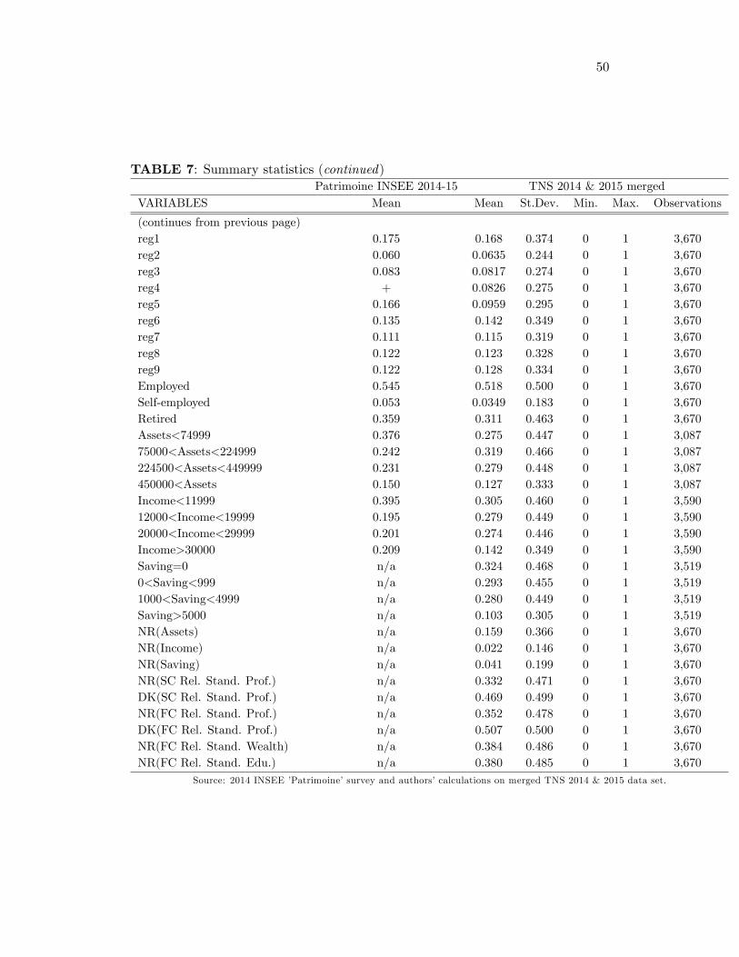
the paper and in Appendix B. Table 7 provides summary statistics for the variables
we use in the analysis.
4. Empirical analysis
Consistent with our theoretical analysis, in which equilibrium depends on the con-
nectedness, k∗i , rather than on the precise identity of interacting agents, we employ
measures of such connectedness in our empirical analysis. Specifically, we focus
on whether and how expectations, perceptions, and behavior are influenced by the
share of the relevant peer circle that the respondent considers informed about or
participating in the stock market.
4.1. Putting the social and financial circles into context. Our assumption
in the theoretical model is that respondents meet their peers and weight the infor-
mation they obtain from them according to how reliable they perceive their peers
to be. In real life, it is natural to think of respondents as forming a financial circle,
in the sense of a subset of their overall social circle with whom they feel confident
to discuss financial matters. Respondents are indeed asked whether they have such
a financial circle, as well as their perceptions regarding attributes of their social
circle and their financial circle, and they separately report their perceptions as to
the shares of both circles that are (i) informed about and (ii) participating in the
stock market. It is important to stress that our data do not record actual shares of
informed or participating peers, which may or may not be known to respondents,
but shares as they are perceived by respondents who form expectations and decide
on own stock market participation and exposure.
For respondents who declare having formed a financial circle, we use expressions
(11) and (12) to compute their implied perceptions regarding members of their social
circle with whom they do not discuss finances. The distinction between a financial
and an outer circle is very useful for checking whether our results might be caused
by unobserved heterogeneity rather than peer influences; and in distinguishing be-
tween exchange of information and mindless imitation of stockholding behavior.
Specifically, it is possible that there are unobserved factors influencing the respon-
dent’s stock market expectations, perceptions or behavior, as well as whether their
peers are informed about, or participating in the stock market. These unobserved
factors might induce a correlation between responses and peer attributes without
implying any effect from peers on respondents. If respondent stock market expec-
19
tations, perceptions, or behavior reflect simply unobserved dimensions along which
respondents are similar to their peers, we would expect correlations to be present,
whether we consider the financial circle or the outer social circle not privy to finan-
cial matters. If, however, only the financial circle, but not the outer circle matters
for subjective expectations, perceptions, or behavior related to stockholding, then
this is evidence against unobserved heterogeneity creating the empirically observed
relationship. Furthermore, the within-respondent variation in peer groups that we
exploit is conditional on variation across respondents in population-wide market
outcomes, to guard against the possibility of social circle selection and unobserved
correlated effects driving our peer effect results, within a highly volatile, effi cient
and competitive market environment.
The split between a financial and an outer circle can also shed some light on
whether social interactions take the form of mindless imitation or exchange of infor-
mation and possibly mindful imitation of peers perceived as knowledgeable about the
stock market. As an example, we would not expect the behavior of the outer circle,
with whom respondents do not discuss financial matters, to influence respondents’
stockholding behavior directly unless there is pure imitation without the exchange
of information. On the other hand, interactions with the financial circle can be in-
formative and contribute to a revision of perceptions about the past performance of
the stock market, expectations about the future, or choices regarding stockholding.
We also note here that the survey questions elicit the shares of informed and
participating peers in the financial and overall social circles only. We use these two
responses to construct the corresponding share of peers in the outer circle, i.e., the
complement of the financial circle to the overall social circle. As our approach is
indirect, it can sometimes lead to outer-circle shares that fall below zero or exceed
100%. When this happens, we adopt a conservative approach to potential inconsis-
tency: we set both the direct response on the financial circle and the implied for
the outer circle to ‘missing observation’, and we introduce an inconsistency dummy
variable (IC) to flag such observations.18 All reported estimates on the two circles
explicitly control for observed inconsistencies in responses.
4.2. Expectations and perceptions. Existing empirical studies of peer effects
on financial behavior focus on outcomes, such as stockholding, retirement saving, or
debt outstanding. We begin our analysis by investigating the role of social interac-
tions for the formation of subjective return expectations about the future, as well
18Exception is made of those inconsistencies that are attributed to rounding, because of lownumbers reported to question D1. With this criterion in place, a total of 19 observations areexcluded from the IC category.
20
as of perceptions regarding past stock market performance. As established, expec-
tations are an important determinant of the demand for risky assets, this analysis
is interesting both in its own right and as a component of the link to stockholding
behavior.19
To investigate the empirical relevance of perceptions regarding interacting peers
for subjective expectations of stock market returns over the next five-year period,
we consider an approximate linear version of expression (8), which suggests two
empirical specifications:
Expec. Ri = κ0 + κ1k∗i + τ iκ+ ei (13)
and
Expec. Ri = κ0 + κ1Dei + τ iκ+ ei, (14)
where k∗i is an indicator of connectedness to the peer circle, Dei is an indicator
of ’expected’or perceived peer behavior (participation in the stock market), τ i is
a vector of individual characteristics which includes individual perceptions about
peer characteristics, ei is an individual zero-mean error term distributed normally
conditional on covariates and the same coeffi cient symbols are used for notational
economy but not to imply equality of coeffi cients.20
Implementing either specification might raise concerns regarding the role of un-
observed heterogeneity. Unobserved factors affecting all peers, including the respon-
dent, could be creating a tendency for peers to be perceived as informed about the
stock market (or as participating in the stock market), and simultaneously for the
respondent to be having higher or lower expectations about future stock market
returns. This could induce a relationship between the share of the social circle be-
ing informed and the reported subjective expectation without any causal implication
running from perceived peer information (participation) to respondent expectations.
As a first approach to handling this problem, we distinguish perceptions about
the two peer circles: the inner, financial circle with whom respondents report that
19Standard models of financial choice under uncertainty predict that decisions should be based onexpectations of future aggregate market outcomes, and not on publicly available information aboutrecent market outcomes, since the latter should be incorporated into respondents’expectations uponconditioning (Brandt, 2010). Indeed, a recent strand of empirical literature finds that subjectiveexpectations are significantly related to financial decisions (e.g. Dominitz and Manski, 2007; Kezdiand Willis, 2009; Hurd et al., 2011).20To control for endorsement peer effects that can rationalize mindless imitation (e.g. due to
a preference to conform), we include measures of the respondent’s perceived relative standing interms of average peer education, average total wealth and professional status with respect to thesocial and financial circles.
21
they discuss financial matters; and the rest of their social circle with whom they
report that they do not discuss such matters. Moreover, we also control for indi-
vidual perceptions of market-wide characteristics unrelated to peer behavior, but
that might be driving asset prices, like an increase in the proportion of the overall
population investing in or being informed about the stock market.
We then investigate whether either share is significantly related to the respon-
dent’s subjective expectation about future stock market returns, after controlling for
a range of observable respondent characteristics. By splitting the social circle into a
financial circle and an outer circle, we are able to apply a ‘double circle’methodology
to identification. Additionally, by including in the controls respondents’perceptions
about population-level behavior, we introduce a novel ‘triple circle’methodology,
with which we explicitly control for both selection of the social circle within the
overall population and for the possibility of correlated, unobserved effects.21 If
unobserved heterogeneity is an important problem, then it should affect both the
financial circle and the outer social circle. Thus, finding different results for the
inner and the outer circles, conditioning on population behavior suggests that the
difference is not due to unobserved heterogeneity, because such heterogeneity would
necessarily have a significant effect on both circles. The empirically implemented
specifications are:
Expec. Ri = κ0 + κ1,FCk∗i,FC + κ1,OCk
∗i,OC + κ1,Pk
∗i,Pop + τ̃ iκ+ ei,
and
Expec. Ri = κ0 + κ1,FCDei,FC + κ1,OCD
ei,OC + κ1,PD
ei,Pop + τ̃ iκ+ ei.
We are able to control for a wide range of characteristics and attitudes of the house-
hold head, τ̃ i. These include individual perceptions about the respondent’s relative
standing in terms of peer characteristics (professional status, education and total
wealth), demographic characteristics (age, gender, marital status, number of chil-
dren), elicited risk preferences (coeffi cient of absolute risk aversion), a proxy for in-
dividual information (self-reported individual perception of the most recent realized
stock market cumulative return), proxies for resources and constraints (educational
21Our ‘triple-circle’methodology separately identifies the effects of the inner, the outer, and thepopulation-minus-social circle outcomes and characteristics on individual behaviour. The necessityof this approach arises from our interest in peer behavior within a competitive market environment.
22
Figure 1: French stock market index, CAC 40, weekly data, 3 March 1990 - 27 June2016. Source: Yahoo Finance.
and achieved liquid saving over the past year), and region of residence.22 In all
specifications, we also include dummies for item non-response and inconsistent re-
sponses, especially to the questions about perceived peer and population behavior.23
Despite the fact that all respondents were asked about the same stock mar-
ket, there is considerable heterogeneity in responses, in both perceptions about its
evolution prior to the data collection and subjective expectations regarding future
stock returns. Figure 1 shows historical monthly data of the French stock market
index CAC-40, from March 1990 to June 2016. The index dropped by nearly 25%
at the time of the sovereign-debt crisis during the second half of 2011. After that
and as we get closer to the time that the two parts of the survey were fielded, the
stock market index was steadily recovering. Both in late December 2014 and May
2015, the index was still below its dot-com and the Lehman brothers peaks, but had
already recovered relative to the sovereign-debt crisis. Given the substantial tur-
moil experienced by the stock market index over the period prior to data collection,
respondents are likely to have been exposed to considerable news coverage of the
stock market evolution, and this makes the observed variation in perceptions and
expectations all the more striking.
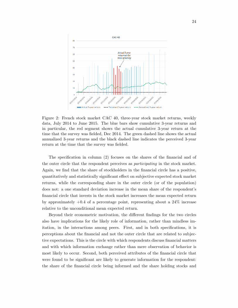
The actual stock market return over the three-year period in question (Dec 2011
22Detailed variable definitions are to be found in Appendix B.23Controlling for item non response to those questions hardly affects the sign, size, and significance
of the main coeffi cients of interest, namely on perceptions regarding peers. A similar robustnessexercise in the presence of missing data can be found in Dimmock, et. al. (2016).
23
- Dec 2014) was +34.57%, but the cross-sectional average perception of respondents
regarding returns over the same period is equal to +3.6%. Figure 2 shows the actual
3-year returns from July 2014 to the June 2015. The average actual 3-year return
in the second half of 2014 was +34.49%. Figure 2 also shows the annualized 3-year
returns for the same period, which are still well above the average perceived returns,
at an average value of 12.43%. Although this average perception gap in stock market
returns seems too wide, it is consistent with rational inattention (Sims, 2003) and is
in line with reported empirical findings on the inflation perception gap of households
(Jonung, 1981; Armentier et al. 2016) and CE/FOs of firms (Coibion, et. al., 2018).
The average cross-sectional subjective expectation of respondents regarding fu-
ture returns is equal to +1.6%. Positive deviations of perceptions from the low
cross-sectional mean and optimism that is greater than the average observed among
respondents of given characteristics in the sample seem consistent with the respon-
dent having more informed perceptions and expectations more in line with available
historical evidence.24
Table 2 reports estimates from these two specifications for subjective expected
returns. The regression specification in column (1) includes, in addition to the
usual household controls, respondent perceptions regarding how informed members
of the two peer circles are. It can be seen that the share of the financial circle
that the respondent regards as informed about the stock market is positively and
significantly related to the respondent’s subjective expectation of future return. The
relationship is quantitatively significant: a one-standard-deviation increase of 17.2
percent in the mean share of a respondent’s financial circle that is informed about the
stock market increases the mean expected return by approximately +0.5 percentage
points (or about a 30% increase relative to the unconditional mean expected return
of +1.6 percentage points). By contrast, the corresponding share of the outer circle
is found to be statistically insignificant. Similarly, for the share of the population
informed. This difference in results suggests that the observed significant correlation
is not simply due to unobserved heterogeneity and creates a presumption in favor
of a causal effect from the financial circle that we will subject to further scrutiny
below.24Dimson, Marsh and Staunton (2008) report a historical (arithmetic) mean excess return (risk
premium) in France for 1900-2005 of around 6% (per annum, p.a), but that figure was reviseddownwards by Le Bris and Hautcoeur (2010) to 2% p.a. when examining a longer time window(1870-2007), correctly weighting for stock market capitalization and adjusting for survivorship bias.Since we are asking respondents about the expected return over a five-year horizon, to be consistentwith the estimate by Le Bris and Hautcoeur (2010) the cross-sectional mean should be 2% p.a. times5 years, or around 10% which is almost an order of magnitude larger than the cross-sectional meanexpected return of 1.6%.
24
Figure 2: French stock market CAC 40, three-year stock market returns, weeklydata, July 2014 to June 2015. The blue bars show cumulative 3-year returns andin particular, the red segment shows the actual cumulative 3-year return at thetime that the survey was fielded, Dec 2014. The green dashed line shows the actualannualized 3-year returns and the black dashed line indicates the perceived 3-yearreturn at the time that the survey was fielded.
The specification in column (2) focuses on the shares of the financial and of
the outer circle that the respondent perceives as participating in the stock market.
Again, we find that the share of stockholders in the financial circle has a positive,
quantitatively and statistically significant effect on subjective expected stock market
returns, while the corresponding share in the outer circle (or of the population)
does not: a one standard deviation increase in the mean share of the respondent’s
financial circle that invests in the stock market increases the mean expected return
by approximately +0.4 of a percentage point, representing about a 24% increase
relative to the unconditional mean expected return.
Beyond their econometric motivation, the different findings for the two circles
also have implications for the likely role of information, rather than mindless im-
itation, in the interactions among peers. First, and in both specifications, it is
perceptions about the financial and not the outer circle that are related to subjec-
tive expectations. This is the circle with which respondents discuss financial matters
and with which information exchange rather than mere observation of behavior is
most likely to occur. Second, both perceived attributes of the financial circle that
were found to be significant are likely to generate information for the respondent:
the share of the financial circle being informed and the share holding stocks and
25
thus knowledgeable about them. The information and participation patterns of the
outer social circle, not deemed reliable for discussion of financial matters, are not
related to stock market expectations of respondents.
In line with the recent literature on inflation expectations by households (Ar-
mentier et al., 2016) and firms (Coibion et al., 2018), columns (3) to (5) of Table
2 introduce subjective perceptions of recent stock price growth (over the past three
years) in the regression of subjective stock market return expectations.25 Answers
to question C42 in our survey enable probabilistic elicitation of respondents’percep-
tions about the most recent realized cumulative stock market return over a three-year
period.26 We focus on the mean of each respondent’s subjective probability distribu-
tion over the size of the realized three-year stock market return. For brevity, we will
be referring to this as the respondent’s perceived return, with the previously intro-
duced notation Perc.R. Consistent with results reported in the literature on infla-
tion expectations, we find that perceived returns are strongly statistically significant
in the subjective expectations regressions, controlling for respondent characteristics
and perceptions about peer characteristics, regardless of whether peer variables are
included in the regression or not. Strikingly, neither the share of informed peers
nor the share of stockholders in the peer circle retain their statistical significance in
the presence of subjective perceptions regarding the recent past return. This finding
suggests that respondent perceptions regarding how informed their financial circle is
or how extensively its members participate in the stock market influence subjective
expectations of future returns only to the extent that they influence perceptions of
recent past returns.
Next, we examine how perceived returns Rit are associated with perceptions
about peer information, k∗i , or group stockholding behavior, Dei , as follows:
27
Rit = Perc. R = η0 + η1,FCk∗i,FC + η1,OCk
∗i,OC + η1,Pk
∗i,Pop + viη + %i, (15)
or
Rit = Perc. R = η0 + η1,FCDei,FC + η1,OCD
ei,OC + η1,PD
ei,Pop + viη + %i, (16)
25Measuring individual information sets is diffi cult even in experimental settings, but someprogress has been made by extending Manski’s (2004) probabilistic elicitation techniques to facts (asopposed to events), as in Arrondel, Calvo-Pardo and Tas (2014), Afrouzi, Coibion, Gorodnichenkoand Kumar (2016) and Coibion, Gorodnichenko and Kumar (2018).26The exact wording of the question, details about the construction of the variable as well as
summary statistics can be found in Appendix B.27This is also in the spirit of Banerjee et al. (2013) or Bursztyn et al. (2014).
26
where %i is an individual zero-mean error term distributed normally conditional
on covariates, vi is a vector of individual characteristics, including individual per-
ceptions about the respondent’s relative standing in terms of peer characteristics
(professional status, education and total wealth), and we use the same symbols for
coeffi cients only for economy of notation and not to indicate equality across spec-
ifications. We report estimates in columns (6) and (7) of Table 2. Interestingly,
we find that perceived past returns are related to the perceived share of financial
circle peers who are informed or who participate in the stock market, but not to the
corresponding features of the outer circle. Quantitatively, a one standard deviation
increase in the mean share of the respondent’s financial circle informed increases the
mean perceived return by around 1.0 percentage point, representing about a 27%
increase relative to the unconditional mean. The respective numbers for participat-
ing in the stock market are 0.8 percentage points, representing approximately a 23%
increase relative to the unconditional mean. This is consistent with our findings in
the expectations regressions that did not control for perceived returns and with the
introduction of such controls rendering the peer circles insignificant.
All in all, results in Table 2 paint a consistent picture: any influence of peers on
subjective return expectations operates through altering perceptions of past returns.
The finding that only the financial and not the outer social circle are related to
perceptions of past returns also suggests that the observed relationship is unlikely
to arise from unobserved heterogeneity, a conclusion that we will return to in what
follows. The identified effects are conditional on relative standing measures of peer
characteristics, none of which are statistically significant. This is consistent with
the view that mindless imitation does not affect expectations of returns.
This first set of results is strongly consistent with the presence of an informa-
tion channel in peer influences running only through the financial circle and only
through perceptions of what happened in the recent past. It also points to a novel
role for friends and acquaintances in enabling respondents to process factual infor-
mation about past stock market outcomes beyond findings in the literature on the
importance of own cognitive ability and financial knowledge for financial behavior.28
4.3. Stockholding. Our preceding analysis of subjective stock market expecta-
tions above has confirmed our model’s prediction (common to models of Bayesian
learning from peers) that connectedness to people more knowledgeable about the
stock market receives a higher weight when forming expectations about stock mar-
ket returns. In addition, more knowledgeable connections raise the reported mean
28See, for example, Christelis, Jappeli and Padula (2010), Grinblatt, Keloharju and Ikäheimo(2011) or Hurd, Van Rooij and Winter (2011).
27
expected return, bringing it closer to available long-run historical estimates (e.g.
Dimson et al., 2008; Le-Bris and Hautcoeur, 2010). Since expected returns are
positively related to desired portfolio exposure to stocks, this alone would suffi ce
to create a role for social interactions in stockholding decisions. In this section,
however, we examine our second prediction, i.e. whether social interactions and
connectedness reduce the posterior variance of returns and thereby increase the
prevalence of stockholding and the degree of exposure to stockholding risk, beyond
its indirect effect through stock market expectations.
Our starting point is the demand for investing in the stock market in expressions
(9) and (10). Reorganizing this indicates that the risk-adjusted individual demands
depend on a term that is common to all agents and a term that is individual-
specific. Since we are exploiting empirically the variation across agents, a linear
approximation of (9) suggests the following econometric specification for agent i’s
share of financial wealth invested in the stock market:
Di = %FWi = max{0, λ0 + λ1(+)k∗i + λ2
(+)Expec Ri + λ3
(−)ρi + τ iλ+ ui}, (17)
where ui is an individual-specific error term. The vector τ i contains individual
characteristics for respondent i, like age, gender, marital status, number of children,
geographical region of residence, employment status, assets, income, borrowing or
liquid savings. It also includes individual perceptions about the respondent’s rela-
tive standing in terms of peer characteristics for both the respondent’s social (profes-
sional status) and financial circles (professional status, education and total wealth)
to capture conformity-driven peer effects on financial behavior.29 In addition, in-
dividual perceptions about population behavior/information are also included as
observable controls for social circle selection effects, as well as for correlated effects
due to aggregate events such as a ‘news shock’or a ‘market trend’. The signs un-
der the constant coeffi cients indicate the theoretically predicted signs: more/better
informed connections reduce the equilibrium posterior variance of expected returns
(coeffi cient λ1), a higher expected net excess return (coeffi cient λ2) and lower risk
aversion (coeffi cient λ3) increase the desired fraction of financial wealth to be in-
vested in the stock market, controlling for individual characteristics.
The zero term within the specification allows for the observed prevalence of
non-stockholders in the population. The empirical literature on stockholding has
dealt with stock market non-participation in two ways. One way is discrete choice
estimation (typically probit and less frequently logit regressions) of the decision
29The detailed definitions of these can be found in Appendix B.
28
whether to hold stocks or not. Non-participation arises when the expected benefit
from participation, which is a function of desired stockholding and the expected
equity premium, does not exceed the participation cost. A second type of empirical
approach invokes tobit estimation of the risky portfolio share. This is typically linked
to the portfolio model by considering that an agent can have a desired portfolio share
that is positive or negative, but the latter is restricted to zero through a constraint
preventing short sales of stock. This offers a possibility to examine the household’s
degree of exposure to stockholding risk, as opposed to focusing only on its presence.30
Note that, in both cases, portfolio demand, stock market expectations, and stock
market perceptions play a potentially important role.
By analogy to our analysis of expectations and perceptions above, we also con-
sider another specification involving behavior among peers. This takes the form:
Di = %FW = max{0, ζ0 + ζ1Dei + ζ2
(+)
Expec Ri + ζ3(−)ρi + τ iζ + wi}, (18)
where Dei represents a feature of the respondent’s social circle, in this case the
extent of peer participation in the stock market, as perceived by the respondent. In
specification (17) we focus on respondents’perceptions about how informed their
financial and outer circles are about the stock market; and in (18) we use their
perceptions regarding stock market participation of the two circles, all of which are
identified relative to the average population information about and participation in
the stock market, as perceived by the individual.
Stock Market Participation. Column (1) of Table 3 presents results for
a participation probit that employs responses on how informed the three circles
are perceived to be. We confirm that subjective expected returns are positively
and significantly related to participation, consistent with existing portfolio models,
even after controlling for a number of household characteristics and for its declared
willingness to take risks, formulated as absolute risk aversion. Interestingly, however,
we find that a one standard deviation increase in the mean share of a respondent’s
financial circle that is informed about the stock market increases the probability of
investing in stocks by 7.4 percentage points, representing about a 34% increase in the
unconditional probability. This provides empirical support for our second prediction,
i.e. that having more/better informed connections reduces the equilibrium posterior
variance of stock returns. However this is not true for either the outer circle or the30This standard approach should be interpreted with some caution, as it reduces stock market
non-participants to frustrated short-sellers of stock. Nevertheless, it is consistent with the use ofan estimator for censored data such as tobit and opens up possibilities for studying the extensivemargin.
29
population average information.
Column (2) repeats the exercise but now uses respondent perceptions as to the
prevalence of stock market participation in the financial and outer circles, as well as
in the overall population. Here the potential for imitation of stock market partici-
pation among peers is clearly present. Imitation of a person whom the respondent
considers worthy of discussing financial matters is likely to be mindful imitation. It
might even not be imitation at all, if the respondent is not influenced by the mere
fact that the members of the financial circle participate in the stock market, but by
the information they are able to provide because they do participate.
However, we also find that stock market participation among the outer circle
has a positive and statistically significant relationship to the respondent’s own de-
cision to hold stocks relative to the perceived overall population participation rate.
Further, from comparing both, we find that a one-standard-deviation increase in
the mean share of the respondent’s financial circle investing in the stock market
increases the probability to invest in stocks by around 6.3 percentage points, repre-
senting about a 30% increase relative to the sample mean proportion of stockholders
of 21.7%; for the outer circle, the respective numbers are an increase in the probabil-
ity to invest in stocks by 4 percentage points, representing a 19.5% increase relative
to the sample mean proportion of stockholders. The finding that respondents are
influenced by the participation of people in their social circle with whom they do
not discuss financial matters indicates that a tendency for conformism and mindless
imitation as regards stock market participation cannot be ruled out.
Columns (3) and (4) pursue further the econometric problem of potential unob-
served heterogeneity creating the observed correlations. In both cases, it is possible
that the observed relationships arise from unobserved factors that influence both
the respondent and the respondent’s peers. Splitting the social circle into finan-
cial and outer circles already provides evidence against unobserved heterogeneity,
but now we have in column (2) a case in which we observe the joint significance of
both circles. Although the population-wide effect is not statistically significant, in
columns (3) and (4), we undertake a placebo test of the hypothesis that the sta-
tistical significance of the peer variables arises from a tendency for members of the
same age and education group living in the same region to behave in the same way
due to unobserved group factors. To this end, we reshuffl e the responses regard-
ing how informed the two circles are and how heavily they participate in the stock
market, respectively. We find that, when each respondent is matched not with his
or her own responses regarding the financial and outer circles, but with those of a
random person in the same age and education group and living in the same area,
30
the coeffi cients on both circles are no longer statistically significant. This supports
the view that the observed correlations in columns (1) and (2) do not arise from
unobserved group factors that affect all members of the same age and education
group who reside in the same area, including the respondent.
Conditional portfolio shares. Columns (5) and (6) of Table 3 adopt a to-
bit specification in order to test for peer influences on the size of the exposure to
stockholding risk in the portfolio, conditional on holding stocks. Symmetrically to
columns (1) and (2), columns (5) and (6) examine the role of perceptions regarding
how informed the two circles are and to what extent they participate in the stock
market, relative to perceptions about the population. Here, the result is the same,
regardless of which feature of the peer circle we consider: higher shares of informed
or participating members of the financial circle are related to greater exposure to
stockholding risk, providing support for the main theoretical prediction. But so does
the share of the outer circle investing in the stockmarket, which now accounts for
about a half of the overall peer effect on the share of wealth invested in the stock-
market: a one-standard-deviation increase in the mean share of the respondent’s
financial circle investing in the stock market, is related to a higher conditional share
of financial wealth invested in the stock market by around 1 percentage point, repre-
senting about a 4.3% increase relative to the sample mean share of 21.41% amongst
stockholders. For the outer circle, the corresponding figure is a higher conditional
share invested by 1.4 percentage points, representing a 6.4% increase relative to the
sample mean. Just as above, we identify financial and outer circle peer effects of
perceptions relative to how respondents perceive the overall population, as a guard
against unobserved social group effects. Columns (7) and (8) support the argu-
ment that the effects identified on the intensive stockholding margin are not due to
unobserved group heterogeneity, by repeating the analogue placebo counterfactual
exercises as reported under columns (3) and (4) for the participation decision. We
also note that the effects on the conditional share are net of the identified peer effects
on subjective expectations.
All in all, the results in Table 4 suggest that exchange of useful information and
possibly mindful imitation are strongly related to whether individuals participate in
the stock market and to the share of financial wealth invested in the stock market,
conditional on participating; yet, we also find some evidence of mindless imitation
of the outer circle.
Robustness. So far, we have subjected our findings of a relationship between
peer information/peer participation and respondent behavior to the scrutiny of dis-
31
tinguishing between the inner (financial) circle and the outer social circle, as well as
of running placebo tests as ways to handle unobserved heterogeneity. In this section
we provide some additional robustness checks in support of our findings.
First, we examine robustness of our results to recognizing that respondents have
a choice of whether to form a financial circle or not, and that this choice may
be taken jointly with the decision regarding stockholding. Specifically, it may be
that people have some unobserved reason to hold stocks and this factor also pushes
them to form a financial circle with whom they can discuss stockholding and other
financial matters. This joint decision could induce the observed correlation between
stockholding and financial sector attributes without any implication of causality
from the financial circle to the respondent’s stockholding behavior. To deal with
this issue, we follow Blume et al. (2011) and we treat group choice and behavior
(within a group) as a set of joint outcomes.31 Specifically, we consider a bivariate
probit model for the choice to participate in the stock market and the choice to
form a financial circle, allowing for correlated unobserved factors influencing the
two choices.32 We estimate the following bivariate probit econometric specification:{Pr(Stocksi > 0) = Φ(λ0 + λ1k
∗iFC + λ2k
∗iOC + λ3k
∗iPop + λ4Expec Ri + λ5ρi + τ iλ)
Pr(FCi > 0) = Φ(ν ′1k∗iSC + ν ′2k
∗iPop + ν ′3Expec Ri + ν ′4ρi + τ iν
′)
(19)
and the corresponding one for peer participation in stockholding as opposed to the
share of informed peers, where we replace k∗ with De. The stockholding participa-
tion probit is modeled as in previous sections. For the probit describing whether
the respondent decides to form a financial circle as a subset of the social circle, we
postulate a set of explanatory variables that include the respondent’s observable
characteristics, the elicited degree of absolute risk aversion, subjective expectations
regarding stock market returns, subjective perceptions about the relative standing
of the respondent’professional status relative to the mean professional status of the
overall circle, and subjective perceptions about the share of members of the overall
social circle that is informed about the stock market as well as the share that is
participating in the stock market.31The standard approach in the literature has been to instrument peer financial behavior; e.g.
Brown, Ivkovic, Smith and Weisbenner (2008) use the one-year-lagged average equity ownershipof nonnative community members’birth states for equity ownership within the community, whenexploiting the variation across Metropolitan Statistical Areas which define communities. Here, wetake the view by Blume et al. (2011) according to which self-selection contains information aboutthe respondent’s preferences, "which will depend on the social interactions that occur in groups overwhich he is choosing". (p.880)32Note that a two-step process, with financial circle formation as the first step, would run into
the diffi culty that having a financial circle is not a prerequisite for holding stocks. Indeed, our datainclude stockholders who do not declare having a financial circle.
32
In principle the more being in the financial circle and discussing financial matters
with the respondent has to do with exchanging information rather than engaging in
mindless imitation, the more we would expect respondents to form a financial circle
when they perceive a larger share of informed peers. Moreover, we would not expect
this decision to be influenced by the share of people they perceive as candidates for
imitation.
Table 4 presents four bivariate probits. Odd-numbered columns correspond to
the stock market participation branches of the corresponding bivariate probits, while
even-numbered columns are the branches depicting the choice of whether to form
a financial circle or not. In regressions (1) and (3), the share of the social circle
participating enters the regression for whether the respondent has a financial circle
or not, while the share of the financial circle participating enters the second leg of
the stock market participation decision. In regressions (2) and (4), the share of
the social circle perceived to be informed about the stock market plays this role,
with the corresponding share of the financial circle participating entering the stock
market participation leg.
The stock market participation results under columns (1) and (3) confirm the
results we obtained earlier, even when we now also allow for a unobserved correlation
in the two decisions: subjective expected returns are positively correlated with stock
market participation, and so are the perceived shares of informed members in the fi-
nancial circle, as well as of the participating members in the financial or outer circles.
The estimates for the corresponding second branches provide additional support for
the presence of informative social interactions: the share of informed members of
the social circle is statistically significant for the choice to form a financial circle,
but the share of participating members is not.
Moreover, Table 4 sheds light on the main concern leading to the bivariate probit
specification, namely that respondents who intend to invest in the stock market
choose, within their social circles, the peers with whom to discuss their own financial
matters. In that case, the error terms ui and νiFC would be highly correlated such
that ui = φνiFC + υi, and the results reported in previous tables would be biased
due to selection. The last three rows in Table 4 report such correlations φ and
the Wald test statistics and associated p-values for different specifications of (19)
considered, and in no case can we reject the null of independence, H0 : φ = 0. In
addition, estimated coeffi cients on the peer variables and on other covariates under
columns (1) and (3) tend to be similar to those in Table 3.
The robustness of our findings to explicit consideration of the joint decision to
have a financial circle and to hold stocks may admit an intuitive interpretation, also
33
in light of Blume et al. (2011, 2015): by conditioning on the share of peers informed
or participating with whom the respondent does not exchange on own financial
matters (i.e. on the outer social circle information or behavior), we are implicitly
controlling for the possibility of selection into the financial circle in specifications
considered in previous sections.33
Another possibility is that the information or behavior of those peers with whom
the respondent does not exchange on her/his own financial decisions (outer circle) is
measured with error. If that were the case, the results reported in Table 2 would be
subject to attenuation bias and the effect of the participation or information of the
outer circle on the individual’s behavior would be biased towards zero. To account
for this possibility, we exploit responses of individuals regarding population partici-
pation in and information about the stock market and treat them as an instrument.
This is because these responses (i) can be excluded from the stockholding equations,
since they are never statistically different from zero, conditional on covariates, and
(ii) are reliable, e.g. for the average stock market participation rate in our sample
of 21.7%, respondents do seem to have on average an accurate perception of 19.39%
(see Table 7 of summary statistics). The results reported at the bottom of Table 5
under even-numbered columns confirm the latter, with quantitatively big estimated
effects and F-statistics above 40 for the first stage regressions of outer circle par-
ticipation or information, as a function of population participation or information
respectively.
Odd-numbered columns in Table 5 report results for stockholdings (columns
1 and 3) and the share of financial wealth conditional on positive stockholdings
(columns 5 and 7), when information from or participation of the respondent’s
outer circle is allowed to be measured with error. Each of the nonlinear models,
i.e. probits for stockholding and tobits for the conditional shares, is estimated
jointly by maximum likelihood, under the null hypothesis of no measurement error.
The Wald χ2(1) reported at the bottom of Table 5 has associated p-values above
20% for all specifications, and thus we cannot reject the null of no measurement
error. The estimated effects in Table 5 are about one order of magnitude larger
than the non-instrumented ones (as reported in Table 2) and are only statistically
significant for the participation and information from the respondents’ financial
circle; nevertheless, because our test indicates no measurement error, the preferred
results are those reported in Table 2.
Finally, to account for the possibility of functional form misspecification error,
33This is supported by the results reported under columns (5) and (7) where the peer effectsfrom the outer circle are mistakenly excluded, resulting in an increase in the correlation in the errorterms of the group selection and the behavior within a group equations.
34
Table 6 reports the results of allowing for interaction terms between inner and
outer circle peer effect behavior or information and expectations of returns, under
columns 3 and 4 for stockholdings, and 7 and 8 for the conditional share, for our
baseline econometric specifications (17) and (18). The interaction terms are never
statistically different from zero, and therefore not reported, while the non-interacted
estimated effects are qualitatively and quantitatively similar to the results in Table 2
(reported again for comparison in Table 6, under columns 1 and 2 for stockholdings,
and under columns 5 and 6 for the conditional share). In fact, the results of the
estimation with interaction terms provide additional support for the presence of
the information channel, since one-standard-deviation increases in expectations (on
stockholdings) are almost twice as big at the extensive margin (77% bigger) and
about 25% larger at the intensive one, relative to the baseline results reported in
Table 2.
All in all, allowing for functional form misspecification, measurement error and
the possibility of selection provide useful robustness checks for our earlier findings
and some additional support for the hypothesis that social interactions have a sig-
nificant informative, rather than purely mindless imitation, content.
4.4. Comparison to experimental evidence. Banerjee et al. (2013) and
Bursztyn et al. (2014) adopt experimental methods to disentangle information from
imitation effects of the social circle. Banerjee et al. (2013) consider a novel microfi-
nance program and replace the unconditional individual probability of participation
by the individual probability of participation conditional on individual information
sourced from friends. Once informed, they find that an agent’s decision to partic-
ipate in the program is not significantly influenced by the fraction of her friends
participating, concluding that the influence of peer participation is mainly an in-
formation effect.34 It is possible to construct an extreme interpretation of their
findings that would be in conflict with ours. Under such an interpretation, if people
are generally aware of the existence of stocks, they should no longer be influenced
by the share of their peers participating in them. Such an interpretation would be
in contrast to our findings.
We opt for a different interpretation, which stresses the nature of the underlying
financial product. The particular microfinance product may have a much higher
probability of participation conditional on awareness than stocks do. To take an
extreme, if practically all people who know about the microfinance product choose to
use it, the value of social links is in transmitting otherwise inaccessible information
34Their work relies heavily both on the identification of the actual network structure and oncontrol over the information spreading through it.
35
and providing more information has no further effects. Yet we know that stock
market participation is quite limited even among the many people aware of stocks
in developed economies. Thus, there is room for further information beyond the
existence of stocks to deliver effects on stock market participation and on the degree
of exposure to stockholding risk.
Bursztyn et al. (2014) adopt a different experimental strategy and find empirical
support for both information and imitation channels. They design a field experi-
ment amongst socially paired investors of a Brazilian brokerage firm, and through
sequential randomization, they separate the effect of a social peer actually purchas-
ing a new financial product from being informed about it. This is accomplished
by randomly informing peers about products, but also controlling whether they are
able to invest in them or not. They are thus able to decompose the total effect of
observing a peer hold a product into one that comes from the information that the
peer is interested in having the product and one that comes from the information
that the peer has been successful in acquiring the product. In this setup with fully
controlled information flows, knowledge that a peer is interested in owning the new
product is the only participation information that the respondent receives, and it
can have a sizeable effect on the respondent’s decision. It is entirely possible that
observing peers participating in a mature and well-known product, such as stocks,
will only have an incremental effect on the respondent’s own decision. The objec-
tive to control the information flow restricts attention to unknown products with
unknown appeal to others.
In our analysis, we deal with a well-known, yet information-intensive product in
a developed economy, namely stocks in France. The more limited role for mindless
imitation in the context of a widely known and mature product such as stocks is
quite intuitive: not much information is added by learning that an extra person
holds it, compared to learning this about a completely novel product.
Mature financial products for which there is limited participation and uncon-
trolled access to information by potential investors abound in developed economies.
Population-wide surveys of behavior relating to such products can provide useful
additional insights to the interesting findings of tightly managed experiments with
new or artificial financial products.
5. Conclusions
We provide a model where purely informative social interactions influence subjective
expectations of future stock market returns as well as the demand for investing in
stocks, within a large effi cient asset market. The model shows that, conditional
36
on investing, individuals collect more information from better informed peers, and
due to the improved precision that this generates, demand more stock in response
to positive pooled signals. By designing, collecting, and exploiting novel survey
data for a representative sample of the French population by age, wealth and asset
classes, collected in December 2014 and May 2015, we find strong support for the
presence of informative social interactions, as well as some evidence for the presence
of mindless imitation of perceived participation behavior in the outer social circle
with whom respondents do not discuss finances.
Based on our findings, the extent to which respondents perceive the financial
circle to be informed about, or participating in the stock market, tends to influence
perceptions of recent returns and only through them, expectations of future re-
turns. Stock market participation and the degree of exposure to stocks, conditional
on participation, are positively influenced by stock market expectations. However,
this is not the only channel through which peers influence stockholding behavior.
Even controlling for subjective mean expectations, stock market participation and
the conditional portfolio share are additionally positively influenced by the extent
to which the financial circle is informed or participating, both of which reduce the
posterior variance of expected returns. We did not find evidence that the corre-
sponding attributes of the outer social circle influence perceptions of past stock
returns or expectations of future returns. These findings are consistent with the
notion that social interactions tend to be, at least in part, informative in relation to
stockholding. However, we did find some evidence for the presence of imitation of
stock market participation observed in the outer social circle. Unlike what happens
with the financial circle, respondents do not discuss financial matters with mem-
bers of this outer circle, and this creates a presumption for the presence of mindless
imitation in the participation decision alongside informative social interactions.
We have followed a three-pronged approach to dealing with unobserved hetero-
geneity being the source of these results. First, we distinguish between attributes of
the financial and of the outer circle: unobserved heterogeneity would tend to make
both relevant rather than only one, as is observed in several of our results. Since
those results are also conditional on corresponding population attributes, selection
and correlated effects should also be less of a concern. Second, we perform placebo
tests, where respondents’perceptions regarding the financial and the outer circle are
reshuffl ed across respondents of the same age, education, and region of residence.
We find that such reshuffl ing eliminates the estimated effects. Third, we adopt a bi-
variate probit specification which recognizes the possibly joint nature of the decision
to hold stocks and to form a financial circle. When we treat group choice and be-
37
havior within a group as a set of joint outcomes, the null of independence among the
two choices cannot be rejected in our sample, and our estimates tend to be similar
regardless of whether we allow for a joint decision or consider stockholding choices
separately. As a final robustness exercise, we use four questions from the TNS2015
questionnaire (questions C5, D6, D7 and D8) that ask respondents to report how
they perceive themselves relative to those in their social and financial circles, in terms
of professional standing, value of their financial assets and qualifications.35 The re-
ported empirical results are conditional on these social utility covariates, which are
never statistically significant, providing further evidence against homophily driving
our model-backed interpretation of the estimated information peer effects.
Informative social interactions imply a potentially powerful channel through
which financial information and financial literacy can permeate through the econ-
omy, even if the original information or financial education content reaches a rela-
tively small segment of the population. They point to a social multiplier in financial
education or financial information even in countries with advanced financial de-
velopment and in products that are mature and widely known, as is the case of
stockholding in France. They provide a (partial or superior) substitute for finan-
cial advice, if ill-conceived, poorly incentivized, or hardly trusted. Finally, they are
likely to grow in importance, as use of social media and the potential to reach more
people with new information spread rapidly. Yet the data also indicate the presence
of some mindless imitation in stockholding. This, along with the inequities involved
in having access to less informed peers, suggest caution in relying exclusively on in-
formative social interactions for the spread of useful information and best financial
practices.
References
[1] Afrouzi, H., O. Coibion, Y. Gorodnichenko and S. Kumar, 2016. Inflation Tar-
geting Does Not Anchor Inflation Expectations: Evidence from Firms in New
Zealand, Brookings Papers on Economic Activity 2015: 151—225.
[2] Armantier, O., Nelson, S., Topa, G., Van Der Klaauw, W. and Zafar, B., 2016.
The Price is Right: Updating Inflation Expectations in a Randomized Price
Information Experiment. The Review of Economics and Statistics.
[3] Arrondel, L., Calvo-Pardo, H., and D. Tas, 2014. Subjective Return Expec-
35For all these questions, respondents answered that less than half of their acquaintances weresimilar to them in terms of assets, qualifications and/or professional standing. See Appendix C,Table 7.
38
tations, Information and Stock Market Participation: Evidence from France.
Southampton Discussion Paper Series in Economics and Econometrics.
[4] Bilias, Y., D. Georgarakos and M. Haliassos, 2010. Portfolio Inertia and Stock
Market Fluctuations. Journal of Money, Credit, and Banking 42(4): 715—742.
[5] Bailey, M., R. Cao, T. Kuchler and J. Stroebel, 2016. Social Networks and
Housing Markets, NBER WP22258.
[6] Banerjee, A., A.G. Chandrasekhar, E. Duflo and M. Jackson, 2013. The Diffu-
sion of Microfinance. Science 341, 1236498.
[7] Beshears, J., J. J. Choi, D. Laibson, B. C. Madrian and K. L. Milkman, 2015.
The effect of providing peer information on retirement savings decisions, Jour-
nal of Finance, 70:1161—1201.
[8] Blume, L. E., W. A. Brock, S. N. Durlauf and Y. M. Ioannides, 2011. Identifi-
cation of Social Interactions. In Jess Benhabib, M. Jackson and A. Bisin eds.,
Handbook of Social Economics, Vol. 1B, ch. 18, North-Holland.
[9] Blume, L. E., W. A. Brock, S. N. Durlauf and R. Jayaraman, 2015. Linear
Social Interactions Models. Journal of Political Economy 123(2): 444—496.
[10] Bordalo, P., N. Gennaioli, Y. Ma and A. Shleifer. 2017. Overreaction in Macro-
economic Expectations. Working Paper, Bocconi University.
[11] Brandt, M. W., 2010. Portfolio Choice Problems. In Y. Ait-Sahalia and L.P.
Hansen, eds., Handbook of Financial Econometrics, Elsevier Science: Amster-
dam.
[12] Brown, J. R., Z. Ivkovic, P. A. Smith and S. Weisbenner, 2008. Neighbors Mat-
ter: Causal Community Effects and Stock Market Participation. The Journal
of Finance 63(3): 1509—1531.
[13] Burnside, C., M. Eichenbaum, and S. Rebelo, 2016. Understanding Booms and
Busts in Housing Markets. Journal of Political Economy 124(4): 1088-1147.
[14] Bursztyn, L., F. Ederer, B. Ferman, and N. Yuchtman, 2014. Understanding
Mechanisms underlying Peer Effects: Evidence from a Field Experiment on
Source: 2014 INSEE ’Patrimoine’survey and authors’calculations on merged TNS 2014 & 2015 data set.
51
APPENDICES, FOR ONLINE PUBLICATION
A. Noisy Rational Expectations Equilibrium
We conjecture that the risky asset price has the form
p = π0 +
n∑j=1
πjxj − γZn, (20)
and imposing market clearing we have that∑
iD∗i = Zn. Let rij = gij/
∑nk=1 gik be
the intensity of the link between nodes i and j, which defines the intensity matrix
R = [rij ] . Then, we can define S ≡ Cov (Rε) = RΣRT ,so that R = K−1G =
K−1AΣ−1,where K is a diagonal matrix with diagonal elements the sums of the
rows of G, i.e. the strengths of the nodes, K = diag [k1, ..., kn] , and therefore
S ≡ K−1WK−1, where the matrix W is defined by W = GΣGT = AΣ−1A. We
note that because A is symmetric and aij ∈ {0, 1} , it is trivially true that
Wii = ki =n∑j=1
aij/s2j .
Finally we make the following assumptions:
A1. ‖W‖∞ = o (n), i.e.
limn→∞
‖W‖∞n
= 0 (21)
A2. limn→∞1n
∑ni=1
kiρi
= β+o (1) . This is slightly modified version of the assump-
tion made by Ozsoylev and Walden (2011). It is written in terms of ki, i.e.
the strength of links, weighted by the risk aversions, but has the same inter-
pretation as in Ozsoylev and Walden (2011), i.e. that the average strength
of nodes weighted by risk aversion (average risk-adjusted connectedness) is β,
and is finite.
A3. The risk aversion coeffi cients come from a distribution such that the harmonic
mean is finite as n→∞, i.e.
limn→∞
n∑ni=1
1ρi
= ρ̂ <∞.
A4. The limit
limn→∞
ki = k∗i <∞
52
exists and is finite. The interpretation of this assumption is that no investor
can be a node with very large strength as the network becomes larger. In other
words, no agent can have too many connections that have very precise signals.
This excludes scenarios of an informationally superior elite in the network.
Under these assumptions can extend Ozsoylev and Walden’s results to the fol-
lowing:
Theorem 1. Under Assumptions A1-A4, with probability 1, the equilibrium asset
price converges to
p = π∗0 + π∗X̄ − γ∗Z̄
where
A =β
ρ̂∆2
π∗0 = γ∗(X̄∆2 + Z̄βσ2
σ2ρ̂∆2 + σ2β
)γ∗ =
σ2ρ̂∆2 + βσ2
βσ2ρ̂∆2 + ∆2 + β2σ2
π∗ = γ∗β
and the optimal demand for the risky asset for an investor i is
D∗i ≡ D∗i (xi, p) =ρ̂
ρi
(X̄∆2 + Z̄βσ2
ρ̂σ2∆2 + σ2β
)− ρ̂
ρi
(∆2
σ2 (ρ̂∆2 + β)
)p+
k∗iρi
(xi − p)
The proof follows the same steps as in Ozsoylev and Walden with some suitable
modifications. The strategy of the proof is to follow the ‘guess-and-verify’approach,
and the main steps are:
1. Conjecture a functional (linear) form for the price, with unknown coeffi cients.
2. Derive beliefs for the agents as a function of the price coeffi cients (using
Bayesian updating).
3. Derive the optimal demands for the agents given their endogenous beliefs.
4. Impose market clearing and solve for the stock price.
5. Impose rational expectations (i.e. equalize coeffi cients) and confirm that the
corresponding system of equation generates a solution, which will then provide
solutions for the price coeffi cients.
53
6. Check, with asymptotic arguments that conditions required to ensure that the
coeffi cients exist (i.e. the system has solution) as n → ∞, are satisfied giventhe assumptions A1-A4.
The detailed steps of the proof are available upon request.
B. Definitions of Variables
Table 7 reports summary sample statistics for all the variables we have used for the
analysis, and compares them to similar measures (when available) in the 2014-2015
Patrimoine INSEE Survey, collected by the French National Institute of Statistics
(INSEE). This is a French Household Wealth Survey, which targets around 20,000
households randomly selected through a process that ensures representativeness of
social categories at the national level. Respondents are interviewed face-to-face,
and are asked to report households’real-estate, financial and professional assets and
liabilities in France. It oversamples the rich (just as most national wealth surveys
do, like the US PSID or the Italian SHIW), and has been fielded in 1986, 1991-1992
(Actifs financiers), 1997-1998, 2003-2004, 2009-2010 and 2014-2015 (Patrimoine)
without a longitudinal dimension. Since 2017, and in partnership with the Banque
de France, it inputs the French part of the Household Finance and Consumption
Survey (HFCS), a harmonized system of wealth surveys supervised by the Euro-
pean Central Bank (ECB). From 2014, the French Household Wealth Survey takes
place every three years, and contains a subsample with a longitudinal dimension.
The new panel establishes, complementary to the face-to-face surveys, a short self-
administered follow-up survey (internet/paper) between waves to reduce attrition.
In addition to describing the distribution of assets and liabilities and their evolution,
the surveys also contain comprehensive information on factors accounting for wealth
accumulation: family and professional biography, inheritances and gifts, income and
financial situation.
B.1. Expec. R. and Perc. R.: Subjective Mean Expectations and MeanPerceptions of Stock Market Returns. To measure expectations, we elicited
probabilistically respondents’beliefs about the cumulative stock market (CAC-40
index) return over a five-year horizon, Pt+5, relative to December 2014, Pt, from the
following question (translated wording):
C39: ‘In five years from now, do you think that the stock market... ’ (For each
category write down how likely the occurrence is by assigning a value between
0 and 100. The sum of all your answers must be equal to 100):
54
... will have increased by more than 25%
... will have increased by 10 to 25%
... will have increased by less than 10%
... will be the same
... will have decreased by less than 10%
... will have decreased by 10 to 25%
... will have decreased by more than 25%
Question C39 inquires respondent i about the subjective relative likelihood of
occurrence, pit+1,k, of each of the seven alternative scenarios, k = 1, ..., 7. Each sce-
nario represents a possible outcome range for the index percentage change between
t and t + 5, Rt+1(5) ≡ Pt+5Pt− 1.36 Questions C40 and C41 provide subjective up-
per and lower bounds for the percentage change, Rimax and Rimin respectively. The
corresponding outcome ranges are:
Rt+1∈
[−Rimin,−25)︸ ︷︷ ︸k=1
, [−25,−10]︸ ︷︷ ︸,k=2
(−10, 0)︸ ︷︷ ︸,k=3
{0}︸︷︷︸,k=4
(0, 10)︸ ︷︷ ︸,k=5
[10, 25]︸ ︷︷ ︸k=6
, (25, Rimax]︸ ︷︷ ︸k=7
and respondents’subjective likelihoods are accordingly:
pit+1,k≡ Pri (Rt+1∈ k) = Pri(Pt+5Pt−1 ∈ k
),∀i
and zero elsewhere, i.e. Rt+1 ∈ (−∞,−Rimin) ∪ (Rimax,+∞). Table 5 reports sum-
mary sample statistics for respondents’answers regarding expectations about stock
market returns, imposing a uniform distribution within the different outcome ranges.
36We follow the standard convention in finance for long-horizon returns, and let 1 + Rt+1(s)denote the stock market index gross return over s periods ahead (hence the subindex t+ 1), whichis equal to the product of the s single-period (or yearly) returns:
1 +Rt+1(s) =s−1∏f=0
(1 +Rt+1+f ) =s−1∏f=0
(It+1+fIt+f
)Similarly, we let 1+Rt(s) denote the stock market index gross return over the most recent s periodsfrom date t− s to date t (hence the subindex t):
1 +Rt(s) =s−1∏b=0
(1 +Rt−b) =s−1∏b=0
(It−bIt−1−b
)See Campbell et al. (1997) for details.
55
On average, households appear more pessimistic and uncertain than the historical
record would predict.
To quantitatively assess how factually informed respondents are, we elicit proba-
bilistically respondents’perceptions about the most recent cumulative stock market
return (CAC-40 index) over the three years, Pt−3, immediately prior to fielding the
survey (December 2014), Pt, as follows (translated wording):
C42: ‘Over the last three years, do you think that the stock market... (For each
category write down how likely the occurrence is by assigning a value between
0 and 100. The sum of all your answers must be equal to 100):
... has increased by more than 25%
... has increased by 10 to 25%
... has increased by less than 10%
... has remained the same
... has decreased by less than 10%
... has decreased by 10 to 25%
... has decreased by more than 25%
Similarly to Question C39, Question C42 asks household i about the subjective
relative likelihood of occurrence, pit,k, of each of the seven alternative scenarios,
k = 1, ..., 7. Each scenario represents a possible outcome range for the percentage
change in the index between t−3 and t, Rt(3) ≡ PtPt−3−1. Probabilistic elicitation of
realized outcomes thus enables us to measure how uncertain they are when conveying
their answers. Since ranges k = 1 and k = 7 are unbounded, we set (Rmax, Rmin) to
match observed values. The outcome ranges for Rt are identical to those of question
C39. Accordingly, households’subjective likelihoods are given by:
pit,k≡ Pri (Rt∈ k) = Pri(
PtPt−3
−1 ∈ k), ∀i
Three years prior to the time when the survey was conducted (December 2011), the
stock market index was only slightly above the floors reached after the dot-com and
Lehman Brothers busts. But, between late December 2011 (CAC 40 = 3159.81)
and late December 2014 (CAC 40 = 4252.29), the index had increased an overall
34.57%. Figure 1 in the main text shows the time window chosen within the wan-
derings of the CAC-40 index between 1990 and 2016. Table 5 reports summary
56
sample statistics for respondents’answers regarding perceptions and beliefs about
stock market returns, imposing a uniform distribution within the different outcome
ranges. A striking finding is that households are on average also pessimistic re-
garding the most recently realized three-year cumulative stock market return (Dec.
2011-Dec. 2014). Although this might be due to imperfect memory given the un-
usually long horizon, it might also be related to the 2007 Lehman Brothers’bust
being overweighted on respondents’memory (Hurd et al., 2011), even if outside the
question’s time window. The big spread around the realized three-year cumulative
stock market perceived return came as no surprise, and it captures factual ambigu-
ity. In addition, it is remarkable that it remains smaller than the spread around the
respectively. Since answers are asked to add up to 100, the reference category
is ’FC Rel. Stand. Profes. =’. About 51% of respondents chose the option
59
to tick the box conveying ‘I do not know’, which informs the corresponding
‘DK(FC Rel. Stand. Profes.)’ dummy variable in Table 5. Non-respondents
account for 35%, and are coded as ‘NR(FC Rel. Stand. Profes.)’
FC Rel.Stand. +Wealth: In the survey (question D7), the respondent is asked
about her/his relative standing in terms of wealth relative to the average
wealth of the respondent’s financial circle, and is given three options: ‘below
the average’, ‘approximately at the average’, or ‘above the average’. Responses
were coded as ordered categories in increasing order from 1 to 3. About 38%
chose not to respond, and are coded as ‘NR(FC Rel.Stand. +Wealth)’in Table
5.
FC Rel.Stand. +Edu.: In the survey (question D8), the respondent is asked about
her/his relative standing in terms of educational attainment relative to the
average educational attainment of the respondent’s financial circle, and is given
three options: ‘below the average’, ‘approximately at the average’or ‘above
the average’. Responses were coded as ordered categories in increasing order
from 1 (below) to 3 (above). Around 38% are non-responses, which are coded
as ‘NR(FC Rel.Stand. +Edu.)’ in Table 5.
B.5. Demographics and other control Variables.
Endowments.
Total wealth: In the survey (question C29), the respondent is asked which of the
ten predefined available brackets corresponds to the household’s non-human
wealth, including housing, estates and professional assets (without excluding
debt):37 ‘Less than 8,000’, ‘between 8,000 and 14,999’, ‘between 15,000 and
39,999’, ‘between 40,000 and 74,999’, ‘between 75,000 and 149,999’, ‘between
150,000 and 224,999’, ‘between 225,000 and 299,999’, ‘between 300,000 and
449,999’, ‘between 450,000 and 749,999’and ‘750,000 or more’. Total wealth
is given in Euros. From the empirical distribution we obtain total wealth
quartiles, the bounds of which are given by ‘74,999’, ‘224,999’and ‘449,999’.
The reference category is the first quartile, ‘less than 74,999’.
37 If we were interested in a continuous measure, we would implement the method of simulatedresiduals (Gourieroux et al. 1987). We would then regress an ordered probit of the respondents’total wealth (bracket) on demographic and socio-economic household characteristics. Once wewould have the estimated total wealth, a normally distributed error would be added. We wouldthen check if the value falls inside the bracket originally chosen by the individual. If not, anothernormal error would be added and so on until we the true interval is correctly predicted. Doingso would allow us to overcome the non-response problem for some households. Would there be amissing value, the predicted value plus a normal error would be directly used.
60
Total financial wealth: In the survey (question C16), the respondent is asked which
of the ten predefined available brackets corresponds to the household’s financial
wealth (excluding housing, estates and professional assets), including cash
and positive balances on checking accounts: ‘Less than 500’, ‘between 1,500
and 2,999’, ‘between 3,000 and 7,999’, ‘between 8,000 and 14,999’, ‘between
15,000 and 29,999’, ‘between 30,000 and 44,999’, ‘between 45,000 and 74,999’,
‘between 75,000 and 149,999’, ‘between 150,000 and 249,999’and ‘250,000 or
more’. Total financial wealth is given in Euros.
Income: For the income of the household, the survey (question A12) asks the re-
spondent which of the nine predefined available brackets better corresponds to
her situation: ‘Less than 8,000’, ‘between 8,000 and 11,999’, ‘between 12,000
and 15,999’, ‘between 16,000 and 19,999’, ‘between 20,000 and 29,999’, ‘be-
tween 30,000 and 39,999’, ‘between 40,000 and 59,999’, ‘60,000 or more’and
‘No income’. Income refers to the respondent’s annual income (earnings, pen-
sions, bonuses, etc.) in Euros, net of social contributions but before personal
income taxes.38 In addition, TNS reports also the net gross monthly income
of the household, in Euros. From the empirical distribution, we obtain the in-
come quartiles the bounds of which are given by ’11,999’, ’19,999’and ’29,999’.
The reference category is the first quartile, ’less than 11,999’.
Occupational status: (of the household head) the TNS 2014 survey asks respon-
dents about their occupation, grouped into five categories: ‘inactive’, ‘un-
employed’, ‘employed’which includes ‘white-collar’ (liberal and managerial
employees) and ‘blue-collar’workers (employees, clerical and manual work-
ers); ‘self-employed’which includes farmers, artisans and shop and business
owners, and ‘retired’. Finally, we group the first two categories into one, the
reference category.
Preferences.
Absolute risk aversion: The following question is asked to the respondent: ‘If
someone suggests that you make an investment, S̃i, whereby you have one
chance out of two win 5000 euros and one chance out of two of losing the
capital invested, how much (as a maximum) will you invest?’ The question
aims at eliciting the taste for risk from each respondent i, with preferences
ui(.), from the following equality:
ui(wi) =1
2ui(wi + 5, 000) +
1
2ui(wi − Zi) ≡ Eui(wi + S̃i)
38When the survey took place, income in France was not taxed at the source.
61
Figure 3: Histogram of responses to the hypothetical lottery that enables elicitation of therespondent’s coeffi cient of absolute risk aversion (CARA) -TNS 2014 survey question C44.
The coeffi cient of absolute risk aversion can be then obtained from a second
order Taylor expansion, as Ai(wi) = 2(5000 − Zi)/(50002 + Z2i ), where Zi is
the amount that the respondent declares to be willing to invest. Those who
declare Zi < 5000 are risk-averse Zi = 5000, are risk-neutral and Zi > 5000
are risk-lovers. The outcome range for the coeffi cient of absolute risk aversion
Ai(wi) is [0, 40]. A total of 3,335 respondents answered the question, with
a mean response of 38.40 and a median value of 39.92. Fig. 3 displays the
histogram of responses, which is very skewed to the left but remains within the
range responses found in the literature. Further details regarding the measure
of absolute risk aversion can be found in Guiso and Paiella’s (2008) work.
Demographics.
Age: it is a continuous variable equal to the age of the household head. Respon-
dents’ age range is in between 19 and 94. We group respondents into four
categories: ‘younger than 35’, ‘between 35 and 49 years old’, ‘between 50 and
64 years old’or ‘older than 65’. Depending on the age bracket within which
respondents’age falls, it takes value 1 within it and zero otherwise.
Gender : it is a dummy variable equal to 1 if the household head is a male, and is
equal to 0, if a female.
Marital status: Marital status is based on current legal marital status. Respondents
who are married or/and living with a partner are coded as 1, and 0 otherwise.
62
Children at home: it is a dummy variable coded as 1 if the respondent replies that
there is (a positive number of) children living at home with their parent(s),
and is coded as 0 otherwise.
Constraints.
Liquidity and borrowing constrained : Respondents are asked if they held an out-
standing (negative) debt balance, and if not, why. We then constructed a
dummy variable that takes value 1 if the respondent answers the question in
the categories ‘because my debt application was turned down’or ‘because I
did not submit an application for fear of being turned down’, and value 0
otherwise.
Saving : Question C73 in the TNS 2014 survey asks the respondent about total net
household saving over the last 12 months. Six brackets are provided, in Euros,
of which the first is zero (’we have not saved’). Around 31% of respondents
report no savings over the last 12 months. From the empirical distribution,
we obtain the saving quartiles the bounds of which are given by ’0’, ’999’and
’4,999’. The reference category is the first quartile.
Region of residence is a categorical variable, with nine possible categories repre-
senting the respondent’s region of residence: ‘reg 1’is Paris, ‘reg 2’is ‘Nord’,