A&A 540, A32 (2012) DOI: 10.1051/0004-6361/201118287 c ESO 2012 Astronomy & Astrophysics Infrared excess around nearby red giant branch stars and Reimers law M. A. T. Groenewegen Koninklijke Sterrenwacht van België, Ringlaan 3, 1180 Brussel, Belgium e-mail: [email protected]Received 17 October 2011 / Accepted 30 January 2012 ABSTRACT Context. Mass loss is one of the fundamental properties of asymptotic giant branch (AGB) stars, but for stars with initial masses below ∼1 M , the mass loss on the first red giant branch (RGB) actually dominates mass loss on the AGB. Nevertheless, mass loss on the RGB is still often parameterised by a simple Reimers law in stellar evolution models. Aims. We study the infrared excess and mass loss of a sample of nearby RGB stars with reliably measured Hparallaxes and compare the mass loss to that derived for luminous stars in clusters. Methods. The spectral energy distributions of a well-defined sample of 54 RGB stars are constructed, and fitted with the dust radiative transfer model DUSTY. The central stars are modelled by MARCS model atmospheres. In a first step, the best-fit MARCS model is derived, basically determining the effective temperature. In a second step, models with a finite dust optical depth are fitted and it is determined whether the reduction in χ 2 in such models with one additional free parameter is statistically significant. Results. Among the 54 stars, 23 stars are found to have a significant infrared excess, which is interpreted as mass loss. The most luminous star with L = 1860 L is found to undergo mass loss, while none of the 5 stars with L < 262 L display evidence of mass loss. In the range 265 < L < 1500 L , 22 stars out of 48 experience mass loss, which supports the notion of episodic mass loss. It is the first time that excess emission is found in stars fainter than ∼600 L . The dust optical depths are translated into mass- loss rates assuming a typical expansion velocity of 10 km s -1 and a dust-to-gas ratio of 0.005. In this case, fits to the stars with an excess result in log ˙ M ( M yr -1 ) = (1.4 ± 0.4) log L + (-13.2 ± 1.2) and log ˙ M ( M yr -1 ) = (0.9 ± 0.3) log (LR/M) + (-13.4 ± 1.3) assuming a mass of 1.1 M for all objects. We caution that if the expansion velocity and dust-to-gas ratio have different values from those assumed, the constants in the fit will change. If these parameters are also functions of luminosity, then this would affect both the slopes and the offsets. The mass-loss rates are compared to those derived for luminous stars in globular clusters, by fitting both the infrared excess, as in the present paper, and the chromospheric lines. There is excellent agreement between these values and the mass-loss rates derived from the chromospheric activity. There is a systematic difference with the literature mass-loss rates derived from modelling the infrared excess, and this has been traced to technical details on how the DUSTY radiative transfer model is run. If the present results are combined with those from modelling the chromospheric emission lines, we obtain the fits log ˙ M ( M yr -1 ) = (1.0 ± 0.3) log L + (-12.0 ± 0.9) and log ˙ M ( M yr -1 ) = (0.6 ± 0.2) log(LR/M) + (-11.9 ± 0.9), and find that the metallicity dependence is weak at best. The predictions of these mass-loss rate formula are tested against the recent RGB mass loss determination in NGC 6791. Using a scaling factor of ∼10 ±∼ 5, both relations can fit this value. That the scaling factor is larger than unity suggests that the expansion velocity and/or dust-to-gas ratio, or even the dust opacities, are different from the values adopted. Angular diameters are presented for the sample. They may serve as calibrators in interferometric observations. Key words. circumstellar matter – stars: fundamental parameters – stars: mass-loss – planetary systems 1. Introduction Almost all stars with masses between 1 and 8 M pass through the asymptotic giant branch (AGB). On the AGB, the mass-loss rate exceeds the nuclear burning rate, implying that the mass- loss process dominates stellar evolution. Although not under- stood in all its details, the relevant process is believed to be that of pulsation-enhanced dust-driven winds: shock waves created by stellar pulsation lead to a dense, cool, extended stellar atmo- sphere, allowing for efficient dust formation. The grains are ac- celerated away from the star by radiation pressure, dragging the gas along (see the various contributions in Habing & Olofsson 2003, for an overview). Following the advent of Spitzer, an anal- ysis of 200 carbon- and oxygen-rich AGB stars in the Small and Large Magellanic Clouds with Spitzer IRS spectra show a clear relation between the mass-loss rate and both the pulsation Appendix A and Table 4 are available in electronic form at http://www.aanda.org period and the luminosity (Groenewegen et al. 2009, and refer- ences therein), confirming earlier work on Galactic stars. The focus of the present paper however is mass loss on the first red giant branch (RGB). For stars with initial masses of < ∼ 2.2 M , this is a prominent evolutionary phase where stars reach high luminosities (log(L/L ) ∼ 3). Low- and intermediate- mass stars must lose about 0.2 M on the RGB in order to explain the morphology on the horizontal branch (e.g. Catelan 2000, and references therein) and the pulsation properties of RR Lyrae stars (e.g. Caloi & d’Antona 2008). For the lowest initial masses ( < ∼ 1 M ), the total mass lost on the RGB domi- nates that of the AGB phase, and therefore it is equally impor- tant to understand how this process develops. In stellar evolu- tionary models, the RGB mass loss is often parameterised by the Reimers law (1975) with some scaling parameter (typically η ∼ 0.4). The RGB mass loss can arise from chromospheric activity (see Mauas et al. 2006; Mészáros et al. 2009; Vieytes et al. 2011) or can also be pulsation-enhanced and dust-driven. The studies Article published by EDP Sciences A32, page 1 of 21
Received 17 October 2011 / Accepted 30 January 2012
ABSTRACT
Context. Mass loss is one of the fundamental properties of asymptotic giant branch (AGB) stars, but for stars with initial massesbelow "1 M#, the mass loss on the first red giant branch (RGB) actually dominates mass loss on the AGB. Nevertheless, mass loss onthe RGB is still often parameterised by a simple Reimers law in stellar evolution models.Aims. We study the infrared excess and mass loss of a sample of nearby RGB stars with reliably measured H!""#$%&' parallaxes andcompare the mass loss to that derived for luminous stars in clusters.Methods. The spectral energy distributions of a well-defined sample of 54 RGB stars are constructed, and fitted with the dust radiativetransfer model DUSTY. The central stars are modelled by MARCS model atmospheres. In a first step, the best-fit MARCS model isderived, basically determining the e!ective temperature. In a second step, models with a finite dust optical depth are fitted and it isdetermined whether the reduction in !2 in such models with one additional free parameter is statistically significant.Results. Among the 54 stars, 23 stars are found to have a significant infrared excess, which is interpreted as mass loss. The mostluminous star with L = 1860 L# is found to undergo mass loss, while none of the 5 stars with L < 262 L# display evidence ofmass loss. In the range 265 < L < 1500 L#, 22 stars out of 48 experience mass loss, which supports the notion of episodic massloss. It is the first time that excess emission is found in stars fainter than "600 L#. The dust optical depths are translated into mass-loss rates assuming a typical expansion velocity of 10 km s$1 and a dust-to-gas ratio of 0.005. In this case, fits to the stars with anexcess result in log M (M# yr$1) = (1.4 ± 0.4) log L + ($13.2 ± 1.2) and log M (M# yr$1) = (0.9 ± 0.3) log (L R/M) + ($13.4 ± 1.3)assuming a mass of 1.1 M# for all objects. We caution that if the expansion velocity and dust-to-gas ratio have di!erent valuesfrom those assumed, the constants in the fit will change. If these parameters are also functions of luminosity, then this would a!ectboth the slopes and the o!sets. The mass-loss rates are compared to those derived for luminous stars in globular clusters, by fittingboth the infrared excess, as in the present paper, and the chromospheric lines. There is excellent agreement between these valuesand the mass-loss rates derived from the chromospheric activity. There is a systematic di!erence with the literature mass-loss ratesderived from modelling the infrared excess, and this has been traced to technical details on how the DUSTY radiative transfer modelis run. If the present results are combined with those from modelling the chromospheric emission lines, we obtain the fits log M(M# yr$1)= (1.0± 0.3) log L+ ($12.0± 0.9) and log M (M# yr$1)= (0.6± 0.2) log(L R/M)+ ($11.9± 0.9), and find that the metallicitydependence is weak at best. The predictions of these mass-loss rate formula are tested against the recent RGB mass loss determinationin NGC 6791. Using a scaling factor of "10± " 5, both relations can fit this value. That the scaling factor is larger than unity suggeststhat the expansion velocity and/or dust-to-gas ratio, or even the dust opacities, are di!erent from the values adopted. Angular diametersare presented for the sample. They may serve as calibrators in interferometric observations.
Key words. circumstellar matter – stars: fundamental parameters – stars: mass-loss – planetary systems
1. Introduction
Almost all stars with masses between 1 and 8 M# pass throughthe asymptotic giant branch (AGB). On the AGB, the mass-lossrate exceeds the nuclear burning rate, implying that the mass-loss process dominates stellar evolution. Although not under-stood in all its details, the relevant process is believed to be thatof pulsation-enhanced dust-driven winds: shock waves createdby stellar pulsation lead to a dense, cool, extended stellar atmo-sphere, allowing for e"cient dust formation. The grains are ac-celerated away from the star by radiation pressure, dragging thegas along (see the various contributions in Habing & Olofsson2003, for an overview). Following the advent of Spitzer, an anal-ysis of 200 carbon- and oxygen-rich AGB stars in the Smalland Large Magellanic Clouds with Spitzer IRS spectra show aclear relation between the mass-loss rate and both the pulsation
" Appendix A and Table 4 are available in electronic form athttp://www.aanda.org
period and the luminosity (Groenewegen et al. 2009, and refer-ences therein), confirming earlier work on Galactic stars.
The focus of the present paper however is mass loss on thefirst red giant branch (RGB). For stars with initial masses of<"2.2 M#, this is a prominent evolutionary phase where starsreach high luminosities (log(L/L#) " 3). Low- and intermediate-mass stars must lose about 0.2 M# on the RGB in order toexplain the morphology on the horizontal branch (e.g. Catelan2000, and references therein) and the pulsation properties ofRR Lyrae stars (e.g. Caloi & d’Antona 2008). For the lowestinitial masses (<"1 M#), the total mass lost on the RGB domi-nates that of the AGB phase, and therefore it is equally impor-tant to understand how this process develops. In stellar evolu-tionary models, the RGB mass loss is often parameterised bythe Reimers law (1975) with some scaling parameter (typically# " 0.4).
The RGB mass loss can arise from chromospheric activity(see Mauas et al. 2006; Mészáros et al. 2009; Vieytes et al. 2011)or can also be pulsation-enhanced and dust-driven. The studies
Article published by EDP Sciences A32, page 1 of 21
of Boyer et al. (2010), Origlia et al. (2007, 2010), and Momanyet al. (2012) of 47 Tuc, and McDonald et al. (2009, 2011) of$ Cen illustrate the current state of a!airs regarding the dustmodelling. Boyer et al. (2010) uses Spitzer 3.6 and 8 µm datato show that the reddest colours on the RGB are reached at thetip of the RGB (TRGB), and that these are known long periodvariables (Clement et al. 2001; Lebzelter & Wood 2005) withperiods between 50 and 220 days. In McDonald et al. (2009),optical and NIR data is combined with Spitzer IRAC and MIPS24 µm data to model the spectral energy distributions (SEDs)and derive mass-loss rates. They conclude that two-thirds of thetotal mass loss is by dusty winds and one-third by chromosphericactivity. They show that the highest (dust) mass-loss rates occurnear the TRGB, which, indeed, are known variable stars beingmostly semi-regular pulsators. At lower luminosities along theRGB, there is an excess at 24 µm that can be translated into amass-loss rate but the uncertainties are large. In an alternativeapproach, using asteroseismology to estimate the mass of redclump stars, and stars on the RGB fainter than the luminosity ofthe clump, Miglio et al. (2012) estimate the amount of mass lostin NGC 6791 and NGC 6819, and conclude that it is consistentwith a Reimers law with 0.1 <" # <" 0.3.
In the present paper, a complimentary approach is taken bystudying the infra-red excess around nearby RGB stars, based ona sample of stars with accurate parallaxes. In Sect. 2, we presentthe sample in addition to the photometric data used to constrainthe modelling. In Sect. 3, the dust radiative transfer models areintroduced, and the results are presented in Sect. 4. Our resultsare discussed in Sect. 5.
2. The sample
We selected our sample from the H!""#$%&' catalog. The paral-laxes were taken from van Leeuwen (2007), and other data forthe stars was gathered from the original release (ESA 1997). Ina first step, supposedly single stars were selected where the pa-rameter fit was good (H!""#$%&' flags isoln= 5 and gof< 5.0).To ensure an accurate determination of the luminosity, a positiveparallax and relative error of smaller than 10% were required(% > 0, &%/% < 0.1).
It is well-established (see e.g. McDonald et al. 2009) thatmass loss is larger in stars near the tip of the RGB but also thatthese stars often show variability. To illustrate this, Fig. 1 showsthe fraction of variable stars across the Hertzsprung-Russell di-agram. We plot 44177 stars from H!""#$%&' that have a parallaxerror of smaller than 15% and an error in (V $ I) of smallerthan 0.15 mag. The cells have a width of 0.1 mag in (V $ I) and0.25 mag in MV . The RGB is clearly visible with a very highfraction of variables. On the basis of this, a further selection of(V$I) > 1.5 (and&(V$I) < 0.1) was imposed. The possible e!ectof using this lower limit to the (V $ I) colour on the fraction ofmass-losing RGB stars is discussed in Sect. 5.1.
At this point in the selection, the interstellar reddeningAV is determined using the method outlined in Groenewegen(2008), which combines various three-dimensional estimates ofAV (Marshall et al. 2006; Drimmel et al. 2003; Arenou et al.1992).
Following Koen & Laney (2000; see also Dumm & Schild1998), the e!ective temperature is estimated from the relationlog Te!(K)= 3.65$0.035 ·(V $ I)0 and the stellar radius (in solarunits) from log R = 2.97$log(%)$0.2·(Vo+0.356·(V $ I)0), fromwhich the luminosity in solar units is then determined. A finalselection using MV < +1.0 (see Fig. 1), 100 < L < 2000 L#,and AV < 0.1 is applied, again to ensure the selection of giants
Fig. 1. The fraction of variable stars in the H!""#$%&' catalog based onthe van Leeuwen (2007) parallax data. The bin size is 0.1 in (V $ I)and 0.25 in MV . Considered are stars with an relative parallax error<0.15 and an error in (V $ I) < 0.15 mag. The RGB stands out ashaving almost 100% variability.
and that reddening will play no role in the interpretation of theresults.
In the section below the methodology is outlined but is basedon fitting models to the SED. Therefore, the availability of suf-ficient photometric data is crucial, especially in the optical andnear-infrared as this will be the main constraint in deriving thebest-fit model atmosphere. For this reason, stars that lacked ei-ther optical UBV and/or JHK data were removed from the sam-ple. In addition, stars that have an IRAS CIRR3 flag> 25 MJy/srwere also removed, in order to avoid contamination by cirrus ofthe IRAS 60 and 100 µm data.
The sample thus selected contains 54 objects (15 of spectraltype K, and 39 M giants) of which the basic properties have beenlisted in Table 1.
Most data listed come from the H!""#$%&' catalog, includingthe type of variability and the di!erence between the 95% and5% percentile values of HP (#HP). In addition, the reddening(see above, Col. 4), the spectral type (from SIMBAD, Col. 7),and both [Fe/H] and log g determinations from the literature(Cols. 10, 11) are listed.
3. The model
The code used in this paper is based on that presented byGroenewegen et al. (2009). In that paper, a dust radiative transfermodel was included as a subroutine in a minimisation code using
Notes. (a) Variability type, Field H52 in the H!""#$%&' (ESA 1997) catalog. Meaning: C = “constant”, not detected as being variable, D = duplicity-induced variability flag, M = possible micro variable, U = unsolved variable, P = Periodic, R = revised colour index. (b) References for [Fe/H] andlog g: (1) Massarotti et al. (2008, and references therein); (2) McWilliam (1990); (3) Cenarro et al. (2007); (4) Fernández-Villacañas et al. (1990).
A32, page 3 of 21
A&A 540, A32 (2012)
the the ($)(!* routine (using the Levenberg-Marquardt methodfrom Press et al. 1992). The parameters that were fitted in theminimisation process include the dust optical depth in the V-band ('V ), luminosity, and the dust temperature at the inner ra-dius (Tc). The output of a model is an SED, which is folded withthe relevant filter response curves to produce magnitudes thatcan be compared to the observations (see Groenewegen 2006).Spectra can also be included in the minimisation process. InGroenewegen et al. (2009) the dust radiative transfer model wasthat of Groenewegen (1993; also see Groenewegen 1995), butthis has since been replaced by the dust radiative transfer modelDUSTY (Ivezic et al. 1999).
The central star was modelled by a MARCS stellar photo-sphere model1 (Gustafsson et al. 2008). Models for temperaturesbetween 3200 K and 4000 K (in steps of 100 K), and those of4250 K and 4500 K, with solar metallicity and log g = 1.5 wereconsidered. Spectroscopically determined metallicites and grav-ities were only available for a third of the sample (Table 1) butindicate that log g = 1.5 is an appropriate value. The medianmetallicity is $0.17 dex, so slightly subsolar.
As the mass-loss rates in RGB stars are expected to be small,and the IRAS LRS spectra (see below) show no hint of a 9.8 µmsilicate feature, two types of dust were considered: aluminiumoxide (AlOx), and metallic iron. The first species is expected asone of the first condensates in an oxygen-rich environment (seeNiyogi et al. 2011, for a recent discussion), while metallic ironhas gained interest in the past few years as a source of opacity(see e.g. McDonald et al. 2010).
Absorption and scattering coe"cients were calculated forgrains of radius 0.15 µm in the approximation of a “distributionof hollow spheres” (DHS) (Min et al. 2005, a vacuum fraction of70% is adopted) using the optical constants of Begemann et al.(1997) for AlOx, and Pollack et al. (1994) for iron.
The SEDs were constructed considering the followingsources of photometry: Mermilliod (1991) for UBV photometry,and the I magnitude as listed in the H!""#$%&' catalog, Gezariet al. (1999) for JHKLM photometry (2MASS was not consid-ered, as owing to the brightness of the sources, the 2MASS pho-tometry was either saturated or had very large error bars), theIRAS Point Source Catalog (PSC, Beichman et al. 1985) andFaint Source Catalog (FSC, Moshir et al. 1989) for 12, 25, 60,and 100 µm data (only data with flux-quality 3 were considered),AKARI IRC (Ishihara et al. 2010) and FIS (Yamamura et al.2010) mid- and far-IR data, In addition, the IRAS LRS spectra(Olnon et al. 1986) available from Volk & Cohen (1989)2 wereused when available. The spectra were typically scaled by fac-tors 1.3–1.6 to ensure that they agreed with the IRAS 12 µmand/or AKARI S9W filter.
In a first iteration, models with e!ectively no mass loss('V = 10$5) were run by varying only the e!ective tempera-ture. A r$2 density distribution was assumed, and the condensa-tion temperature was fixed at 1000 K in all models, as this can-not be constrained from the current photometric datasets for lowmass-loss rates. The best-fit model was determined. In a seconditeration, for that e!ective temperature, models with fixed opti-cal depths of 'V = 10$4, 10$3, 10$2 were run for both iron andAlOx dust. The best-fit model was determined (thus fixing thedust component), and then models where ' was also allowed tovary were run. Finally, models were run in which ' was allowedto vary using e!ective temperatures one step cooler and hotter inthe available grid of MARCS models.
Table 2 lists the parameters of the models that provide the bestfit to the observed data. The fit error in the derived optical depthis typically small, in the median only 5%, but in some casesmuch larger. However, this error does not take into account e.g.the e!ect of varying the model atmosphere. Some tests wereperformed by varying the gravity of the model atmosphere by±0.5 dex and the metallicity by ±0.25 dex and refitting theoptical depth. The results suggest that this represents an addi-tional 50% uncertainty. The largest uncertainty is in the conver-sion from optical depth to mass-loss rate. On the one hand, asystematic error as the mean velocity and mean dust-to-gas ratiomay di!er from the adopted values, and, on the other hand, thevalues for individual stars will scatter around these mean values.A random error of a factor of two is adopted in the latter case,and this error dominates the error budget.
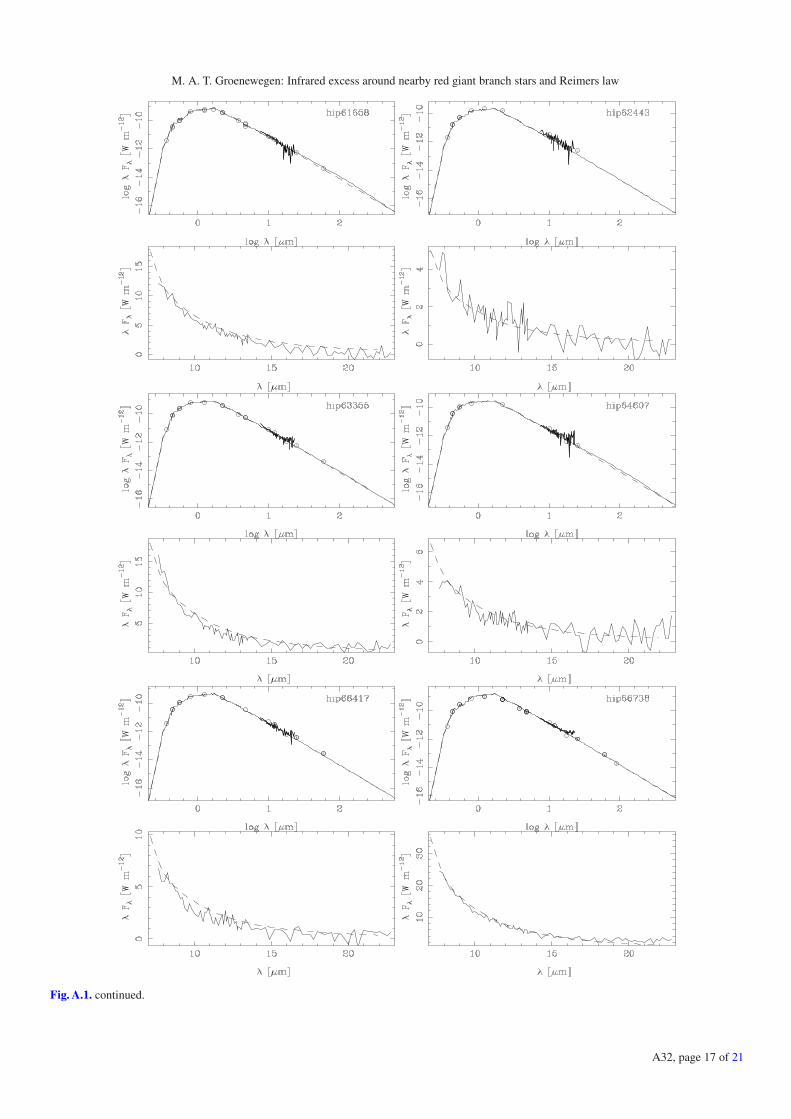
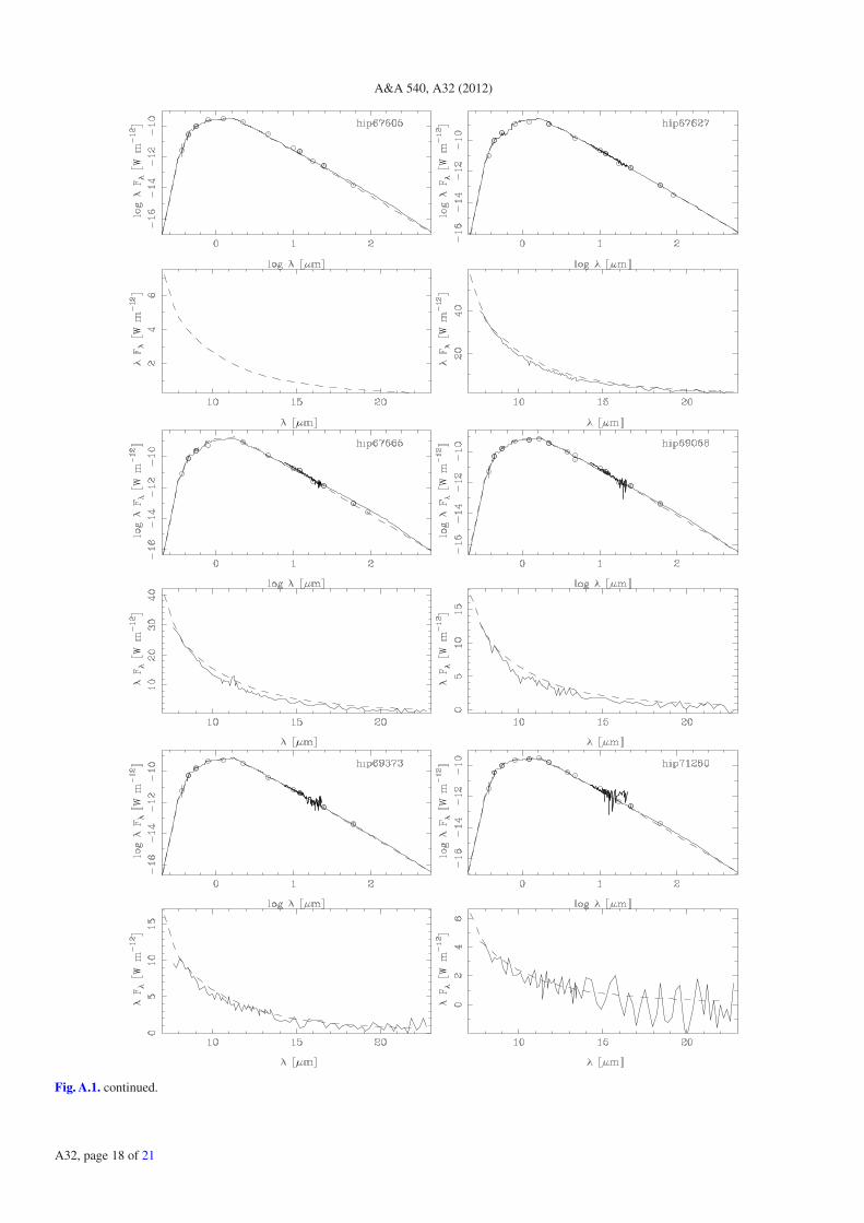
Examples of the fits are shown in Fig. 2, and all fits are dis-played in Appendix A. The panels with the SEDs show the bestfit (solid line), and a model without mass loss (dashed line) forcomparison. The di!erences are often small, certainly visually,but are statistically significant.
From inspecting the plots, it is also clear that far-IR data("80–200 µm) would certainly be very valuable in constrain-ing the models, as any excess is expected to be largest in thatwavelength region. In this respect, it is unfortunate that theAKARI/FIS has relatively poor sensitivity. All 54 stars haveAKARI/IRC S9W and L18W data, but only 15 have FIS WS-band data at 90 µm and none of the stars are detected in the filtersat 140 and 160 µm. None of the stars are detected in the PlanckEarly Release Compact Source Catalogue (Planck Collaboration2011), no appear to have MIPS or Herschel data.
In addition, high-quality mid-IR spectra would also be usefulto improve upon the, in most cases, relatively poor quality IRASLRS spectrum. Only for one object does an ISO SWS spectrumexist (HIP 87833 = ( Dra). With the current data, no clear dustfeature is visible in any of the stars, hence, when a significant in-frared excess detected, the best fit is provided by the featurelessmetallic iron model rather than the aluminium oxide one (exceptin one case).
Other mechanisms can produce an infrared excess that is notdue to dust emission, as discussed in MacDonald et al. (2010),e.g. free-free emission or emission from shells of molecular gas(a MOLsphere; e.g. Tsuji 2000). Even featureless dust emissioncould in principle also be due to extremely large ("50 µm) sil-icate or amorphous carbon grains (MacDonald et al. 2010), butthese species are not really expected to condense and form firstin these low-density oxygen-rich CSEs.
Free-free emission is ruled out by MacDonald et al. (2010)as an important source of emission in their sample of giants in $Cen. A MOLsphere could be due to many molecules but wouldmost likely manifest itself by the presence of water lines in the6–8 µm region. This region is not covered by the LRS spectrumso it is impossible to verify this idea directly. MacDonald et al.(2010) studied the e!ect of using Spitzer IRS data and found thatno reasonable combination of column density and temperaturecould reproduce the flatness of their spectra. For red supergiants,which are much more luminous that RGB stars but that have sim-ilar e!ective temperatures than the stars under study, Verhoelstet al. (2006, 2009) found that a MOLsphere alone cannot explainthe excess emission in the mid-IR and that a additional source ofopacity was needed.
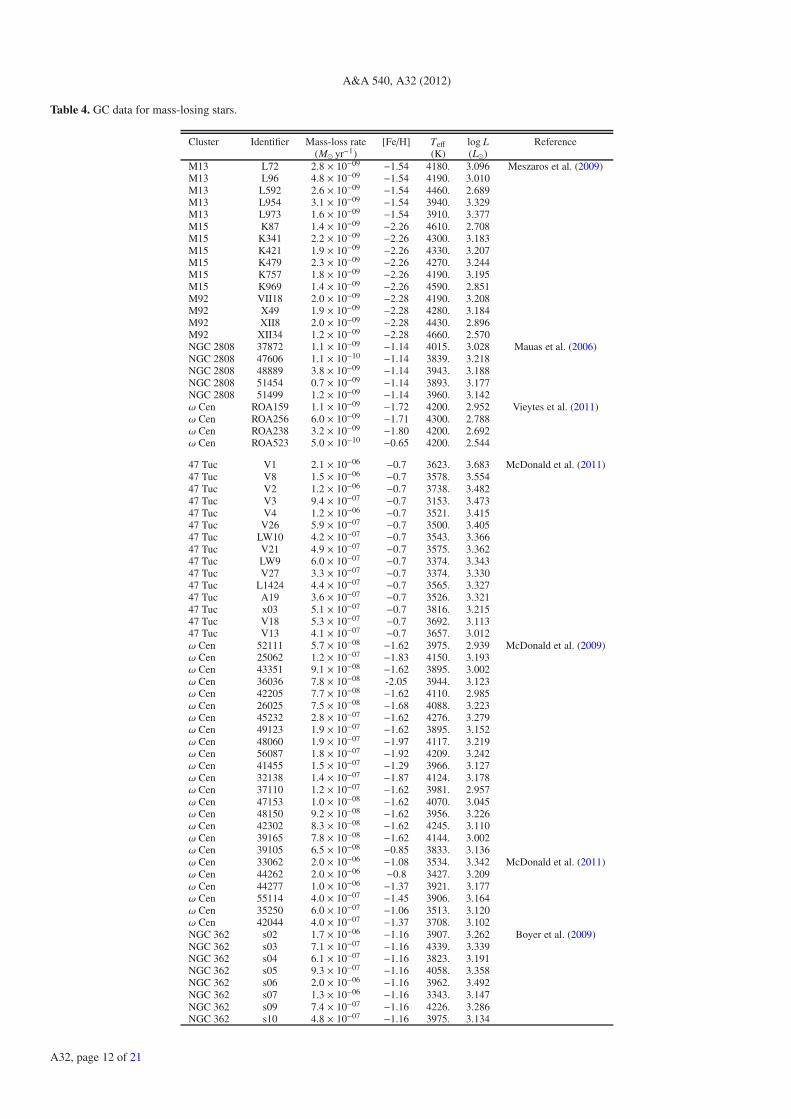
Notes. Listed are, (Col. 2) the e!ective temperature of the MARCS model, (Col. 3) the dust component that fits best in the case when 'V ! 10$5,(Col. 4) luminosity and the internal error (that is, the error in the H!""#$%&' distance is not included), (Col. 5) the angular diameter in mas andthe error (based on the error in L, and a 70 K error in Te!), (Col. 6) the dust optical depth in the V-band and the internal error, and (Col. 7) thecorresponding mass-loss rate assuming a constant expansion velocity of 10 km s$1, a dust-to-gas ($) ratio of 0.005 and grain specific density, *,of 5.1 g cm$3 (appropriate for iron grains in a DHS with 70% vacuum), (Col. 8) a code if the optical depth was fitted (1) or fixed (0), (Col. 9) thereduced !2 to indicate the goodness of the fit.
A32, page 5 of 21
A&A 540, A32 (2012)
Fig. 2. Example fits to the SED (top panel) and IRAS LRS spectra (lower panel). In the top panel, the solid line indicates the best fit, the dashedline the model without mass loss. For HIP 4147, the best-fit model is the model without mass loss so that the two lines are over-plotted. Theobserved photometry is plotted by the circles, and error bars are also plotted, but are typically much smaller than the symbol size. In the lowerpanel, the best-fit model is indicated by the dashed line, and the LRS spectrum by the solid line. Sometimes no LRS spectrum is available, as forHIP 52366. The complete figure is available in Appendix A.
Fig. 3. Mass-loss rate plotted against LR/M (for a mass of 1 M#) and L. Stars for which no mass loss could be detected (an optical depth of10$5) are plotted as crosses. The solid lines indicate least squares fits to the data (see Table 3), while the dashed line represents Reimers law with# = 0.35. The cross in the lower right corner indicates a typical error bar.
5. Discussion
5.1. Mass loss
Reimers law represents the Reimers (1975) mass-loss rate for-mula for red giants given by
M = # 4 % 10$13!LR
M
"((M# yr$1),
(with ( = 1 and # = 1, and L, R and M in solar units) which,interestingly, Kudritzki & Reimers (1978) updated to M = (5.5±1) % 10$13 L·R
M (M# yr$1), i.e. # & 1.4, by considering the massloss in + Her, + Sco, and ,2 Lyr.
The left-hand panel of Fig. 3 shows the results of the currentwork, assuming a mass of 1.1 M# for all stars. The PARAM tool3(da Silva et al. 2006) was used to find that this is the typical massof a star in the sample. An unweighted least squares fit giveslog M (M# yr$1) = (0.9 ± 0.3) log(L R/M) + ($13.4 ± 1.3). Theslope is consistent with unity, but the coe"cient (3.7%10$14) is afactor of ten lower than in Reimers law. When ( is fixed to unity,the coe"cient becomes 1.8 % 10$14 (# & 0.04) with an error ofa factor of 3.4. The right-hand panel shows a fit of the mass-loss rate versus luminosity log M (M# yr$1)= (1.4 ± 0.4) log L +($13.2 ± 1.2). Similar plots were made with the sample dividedinto K- and M-giants, according to H!""#$%&' variability typeand e!ective temperature, but no clear trends were found. Fits
Notes. First entries are fits to the current sample (see Fig. 3). Last three entries includes literature mass-loss rates from modelling chromosphericlines in GC RGB stars (see Fig. 4).
against radius and e!ective temperature have also been made,and the results are compiled in Table 3. The best-fit relation isobtained when the mass-loss rate is fitted against (log) stellarradius.
Linear fits using two variables were also tested (Table 3),which resulted in lower !2 but, according to the Bayesian infor-mation criterion (Schwarz 1978) where BIC = !2+ (p+1) ln(n)(p is the number of free parameters, and n the number of datapoints), this is not significant as the BICs are larger.
These trends are in agreement with Catelan (2000), who inhis appendix also presents several simple fitting formula that fitthe data equally well. In the case of the fit against radius (hisEq. (A3)), he finds a slope of 3.2 (no error given), while we finda similar value of 2.6 ± 0.7. For a radius of 100 R#, Catelans’formula gives a mass-loss rate of 3.0% 10$9, while we find 2.2%10$9 M# yr$1.
Among the 54 stars, 23 stars are found to have a significantinfrared excess, which is interpreted as evidence for mass loss.The most luminous star with L = 1860 L# is found to have massloss, while none of the 5 stars with L < 262 L# show evidencefor mass loss. In the range 265 < L < 1500 L#, 22 stars out of48 show mass loss, which supports the notion of episodic massloss proposed by Origlia et al. (2007). They also find a shal-lower slope of ( = 0.4, which the current data does not support.Catelan (2000) quotes ( = 1.4.
The sample selection discussed in Sect. 2 involved imposinga lower limit of (V$ I)0 > 1.5, which could lead to a bias favour-ing mass-losing stars. To verify this, the (V $ I) colour predictedby the RT model of the mass-losing stars was compared to thecolour of a model with the optical depth fixed to zero. Even forthe star with the highest mass-loss rate, the model without massloss is only bluer by 0.003 mag. This implies that the selectionbased on (V $ I) has no consequences for the statistics of thenumber and fraction of mass-losing stars in the sample.
Mass-loss rate estimates below the tip of the RGB existmostly for stars in globular clusters (GCs), derived by both mod-elling the SEDs, as in the present paper, and modelling the chro-mospheric line profiles. Data were collected from the literatureand are reproduced in Table 4. The first 24 entries are based onthe modelling of the chromospheric line profiles, followed bythe results of modelling the SEDs. For $ Cen, the values fromMcDonald et al. (2011) of the mass loss are preferred over thoseof McDonald et al. (2009) as they used Spitzer IRS spectra asadditional constraints in the fitting.
All the SED modelling was performed in a similar way,also using DUSTY. However, in the McDonald et al. (2009,2011, 2011) and Boyer et al. (2009) papers, DUSTY wasrun using a mode assuming radiatively-driven winds (“densitytype= 3”). The output velocity of DUSTY was then scaled as(L/104)(1/4)($/0.005)(1/2)(*/3)($1/2), and the mass-loss rate as(L/104)(3/4)($/0.005)($1/2)(*/3)(1/2). A dust-to-gas ratio of $ =0.005 ·10[Fe/H] was assumed in these models, which correspondsto very low outflow velocities: Boyer et al. (2009) mention val-ues between 0.5 and 1.3 km s$1 for NGC 362, and McDonaldet al. (2011) list values between 0.5 and 3.0 km s$1 for theirsample in $ Cen.
Figure 4 is similar to Fig. 3 but with the literature data nowadded. There is excellent agreement with the mass-loss ratesbased on the modelling of the chromospheric activity, but anapparent discrepancy with the data that are also based on mod-elling the SEDs. This discrepancy is discussed in more detail inSect. 5.2.
The results of unweighted least squares fits to the mass-lossrates derived in the present work and modelling of the chromo-spheric activity are reported in Table 3 and shown in Fig. 4.Adding the data from the chromospheric modelling leads to shal-lower, more accurately determined, slopes.
The use of unweighted least squares fits may be an over-simplification as both the abscissa and ordinate have (di!erent)error bars. The error in the mass-loss rate is di"cult to quantify.Following the discussion in Sect. 4, the internal fit error in theoptical depth (typically 5%), the error in the optical depth dueto uncertainties in the stellar photosphere parameters (typically50%), and the uncertainty in the expansion velocity and dust-to-gas ratio when converting optical depth to mass-loss rates (as-sumed to be a factor of 2) are added in quadrature. The last errorterm dominates.
The error in the mass-loss rate derived by modelling thechromospheric lines is quoted to be a factor of two by Meszaroset al. (2009) and this is taken to be the error for all mass-lossrates derived by modelling the chromospheric lines. This meansthat the error bars along the ordinate are quite similar for all ob-jects used in the fitting.
For the stars studied in the present work, the error in lumi-nosity was derived by adding in quadrature the internal fit error(Table 2) and the error in the parallax (Table 1). The error inradius was calculated by taking the error in L and a 70 K errorin e!ective temperature. The error in mass was assumed to be
A32, page 7 of 21
A&A 540, A32 (2012)
Fig. 4. As Fig. 3, but now for: this work (filled triangles, and the stars without excess as crosses), other data based on SED modelling: 47 Tuc(filled squares), $ Cen (filled circles), NGC 362 (filled stars), and modelling of chromospheric lines: M13 (open stars), M15 (open diamonds),M92 (open triangles), and $ Cen (open circles). The fit is to the present sample and the mass-loss rates from modelling the chromospheric lines,while the dashed line represents Reimers law with # = 0.35. The cross in the lower right corner indicates a typical error bar.
0.1 M#. For the stars in the present sample, typical error barsin log L and log LR/M are 0.026, respectively 0.05 dex, and areshown in Fig. 3.
For the stars in the GCs it turns out that the luminositiesquoted in the literature have been determined from V and K mag-nitudes and bolometric corrections. In addition there is the un-certainty in the distance modulus to the cluster. We assumed thatan error bar of 0.15 in Mbol was representative. The error in ra-dius was calculated as before, while the error in mass was takenas 0.01M#. The typical error bars in log L and log LR/M are 0.06and 0.07 dex, respectively.
The “bivariate correlated errors and intrinsic scatter” (BCES)method was used (Akritas & Bershady 1996)4, assuming thatthe errors along the ordinate and abscissa are uncorrelated. Theresults are very similar to those for the unweighted fitting, seeTable 3, probably because the errors along the ordinate are sim-ilar for all data, and the errors along the abscissa are smallerthan those in the ordinates. In what follows, the results from theBCES method are used.
5.2. Are the winds dust driven?
Figure 4 highlights an apparent discrepancy between the presentwork and the literature data also based on modelling the SEDsand that use the same numerical code.
The di!erence can be traced back to the way in whichDUSTY is run, either with “density type= 1” and assuming a r$2
density law, the mass-loss rate derived from the optical depth,the assumed dust-to-gas ratio and expansion velocity (as in thepresent paper), or, with “density type= 3” (which assumes thewinds are driven by radiation pressure on dust), and then takingthe DUSTY output for the mass-loss rate and expansion velocity,and applying scaling relations (see above) that take into accountthe luminosity and dust-to-gas ratio.
As a test, DUSTY models with “density type = 3” were alsorun for the present sample. The (scaled) mass-loss rates werethen compared to the mass-loss rates from Table 2 scaling thoseto the predicted expansion velocities. Neglecting four outliers(with ratios above 100, which are among the five stars with thelowest mass-loss rates, hence optical depths that are probablyparticularly uncertain), the ratio of the mass-loss rates are be-tween 18 and 60, with a median of 38.
Fig. 5. As Fig. 3, with mass-loss rate plotted against luminosity, withmass-loss rates for the current sample calculated using DUSTY in“density type= 3”.
Figure 5 shows the new results together with the literaturemass-loss rates from the SED modelling. The results appear nowto be in much better agreement. We note that this suggests thatthere is a weak if any dependence of RGB mass loss on metallic-ity. The agreement between the mass-loss rates from the presentmodelling and the chromospheric line emission of the GC starsindicates the same.
There is however a good reason to be cautious when usingDUSTY in the dust-driven wind mode and that is that the ratioof radiative forces to gravitation may be less than unity in somecases.
Equation (15) in Elitzur & Ivezic (2001) derived this ratio tobe % = 45.8 Q"&22L4/M, where M is the stellar mass in solarunits, L4 the luminosity in units of 104 L#, Q" is the Planckaverage at the stellar temperature of the e"ciency coe"cient forradiation pressure (Eq. (4) in their paper), and &22 is the cross-section area per gas particle in units of 10$22 cm2 (see Eq. (5) intheir paper). The latter quantity can be written as (with Eq. (86)in their paper) &22 = 125.4$/(* a), with $ the dust-to-gas ratio,* the grain specific density in g cm$3, and a the grain size inmicron.
In the optically thin case, Q" can be taken as the sum ofabsorption and scattering coe"cients at the wavelength wherethe stellar photosphere peaks. For the typical e!ective tempera-tures considered here, this is at about 1.6 micron, and Q" " 2.2(for the iron dust properties discussed in Sect. 3). With * = 5.1,a = 0.15 and $ = 0.005, &22 equals 0.82, and then, assuming
M = 1, % becomes 8.3 for L4 = 0.1. In this case, % > 1 and sothe condition to drive the outflow by radiation pressure on dustis met. For the lowest luminosities in which we detect an excess,L is "260 L# and so % " 2.
In the case of the GC stars from the literature, the majorityof luminosities are above L4 = 1 (see Fig. 4) but these authorsassumed the dust-to-gas ratio to scale with metallicity, whichresults in very low values in the range 1/1200 to 1/5000 in thecase of $ Cen (McDonald et al. 2011), and again, % would beclose to or even below unity.
The largest uncertainty in predicting % may be in the calcu-lation of the dust properties. As mentioned in the introduction,there are indications that metallic iron may be abundant and thefact that the infrared excess is featureless is one of them.
A value of Q" = 2.2 is much larger than that found forstandard silicates or carbon dust (Table 1 in Elitzur & Ivezic2001, lists 0.1 and 0.6, respectively, for 0.1 µm sized grains).The adopted grain size is of importance. In the standard case,Q/a = 14.6 µm$1, but this value decreases (and hence % de-creases) to 9.4 and 6.1 for a = 0.1 and 0.05 µm, respectively.This e!ect can also lead to a larger %: Q/a peaks at 21.6 µm$1
for a = 0.23 µm . The influence on grain size is largely due to thescattering contribution and this implies that even the assumptionof isotropic scattering can play a role. The assumption on thegrain morphology is also important. If the DHS is used with asmaller maximum fraction of vacuum Q/(a*) is also reduced:by a factor of 2 in the case of fmax = 0.4 and a factor of 3.2 inthe case of fmax = 0.0 (i.e. compact spherical grains).
Elitzur & Ivezic (2001) derive in a similar way a more strin-gent constraint on the minimal mass-loss rate (their Eq. (69)),M >" 3%10$9 M
Q" &222L4T 0.5
k3, which corresponds to 2%10$8 M# yr$1
for the above values for M,Q", and &22, L4 = 0.1, and Tk3 = 1,which is the kinetic temperature at the inner radius in units of1000 K. On the basis of this consideration. all mass-loss rates inTable 2 are below this critical value.
5.3. Angular diameters
Angular diameters are a prediction of the radiative transfer mod-elling through the fitting of the luminosity and the e!ective tem-perature. The values are listed in Table 2. The (limb darkened)angular diameters of some stars determined from interferometryand the predicted values from the SED modelling are comparedin Table 5.
The largest overlap is that with Bordé et al. (2002),which is based on the results by Cohen et al. (1999).The overall agreement is good, leading to ()Borde et al $)present work)/(
#&2
Borde et al + &2present work) of $1.0± 1.7. There are
2 stars where the di!erence is more than 3&, HIP 44857 andHIP 88122. In the latter case, this is due to the di!erent adoptede!ective temperatures, 4000 K in the present paper, and 3690 Kin Bordé et al., which is the largest di!erence in temperatureamong the 19 stars in common.
The overlap with Mozurkewich et al. (2003) occurs for threesources, for which the agreement is satisfactory. These authorsobtained their data mostly at 550 and 800 nm and therefore thelimb-darkening correction is relatively large. The main di!er-ence is found for HIP 87833, for which Mozurkewich et al.quote angular diameters based on the infrared flux method of10.450 (Bell & Gustafsson 1989) and 10.244 mas (Blackwellet al. 1990), which are in excellent agreement with the presentwork. Finally, two stars overlap with Richichi et al. (2009), andthe agreement is satisfactory.
6. Summary and conclusions
We have selected a sample of 54 nearby RGB stars, and con-structed and modelled their SEDs with a dust radiative trans-fer code. In about half of the stars, the SEDs were statisticallybetter fitted when we included a (featureless) dust component.The lowest luminosity is which a significant excess was found is267 L# (HIP 64607), which is lower than for any other star (asfar as I am aware).
A32, page 9 of 21
A&A 540, A32 (2012)
Table 6. Mass lost on the RGB for a 1.6 M# star.
Relationship #M M (at L = 1000 L#) Remark(M#) 10$9 M# yr$1
The results are compared with mass-loss rates estimated forRGB stars in GCs, based on modelling chromospheric line emis-sion and the dust excess. There is good agreement with the for-mer sample, and fits of the mass-loss rate against luminosityand (L R/M) (Reimers law) are presented by combining thepresent work with the mass-loss rates from the chromosphericmodelling. The derived slope is shallower then in Reimers lawand with a larger constant. The comparison with the literaturevalues based on modelling the dust excess has led to an inter-esting observation. This is that there is a significant di!erenceamong (and dependence on luminosity for) the mass-loss ratesderived when running the DUSTY code in “density type = 1”and assuming a r$2 density law, and then deriving the mass-lossrate from the optical depth, an assumed dust-to-gas ratio, and ex-pansion velocity (as in the present paper), or, with “density type= 3” (that assumes the winds are driven by radiation pressureon dust), and then taking the DUSTY output for the mass-lossrate and expansion velocity, and applying scaling relations thattake into account the luminosity and dust-to-gas ratio (as donein the literature). The origin of the di!erence is unclear, but itturns out that the ratio of radiative forces to gravitation (%) couldbe smaller than unity under certain conditions for the RGB starswe consider, for low luminosity and/or low dust-to-gas ratios (asassumed in the GC stars). In addition, the details of the dust thatforms (iron dust has been assumed in the nearby RGB stars, as itis found to be the dominant dust species in the GC sample), andthe typical grain size and morphology could play a crucial rolein whether % is larger than unity in any given star. This might ex-plain why only 22 out of 48 RGB stars with 265 < L < 1500 L#have an infrared excess. The condition % > 1 may only be ful-filled for 50% of the time (or, instantaneously, in 50% of thestars) in this luminosity range when certain conditions are met.What these conditions or triggers are remains unclear: they couldbe related to either pulsation or convection or be more indirect asfor binarity or magnetic fields. Determining the outflow veloc-ity of the wind for the stars that show an excess would be helpfulbecause this would not only remove the assumption of a constantvelocity of 10 km s$1 for all objects, but also test the predictionsof the dust-driven wind theory.
To investigate the implications of the mass-loss rate for-mula derived here, we compared the predicted mass loss onthe RGB to the recent determination from asteroseismologyfor the cluster NGC 6791 (Miglio et al. 2012), who derivea mass loss of #M = 0.09 ± 0.03 (random)± 0.04 (system-atic) M#. Evolutionary tracks were used from the same dataset(Bertelli et al. 20085) and with the same composition (Z = 0.04,Y = 0.33) as used by Miglio et al. For a star with initial mass
5 http://stev.oapd.inaf.it/YZVAR/
1.6 M# (Miglio et al. determine the mass on the RGB to be1.61 M#), the mass lost on the RGB was calculated when theluminosity was above 250 L# (the e!ect of including the entireRGB is negligible) for di!erent mass-loss recipes (see Table 6).The first entry is for Reimers law with a scaling of # = 0.35,which gives a total mass lost on the RGB close to the observedvalue. The following rows provide the predictions from the best-fit relations derived in this paper with L and LR/M as vari-ables and varying the slope and zero point by their respective1& error bars. Both type of relations can equally well result inthe observed mass lost, for a slope and/or zero point slightlylarger than the best-fit value. As for the scaling of the Reimerslaw, the following relation would fit the observed mass loss of0.09 ± 0.05 M# equally well: M = #11.25 % 10$12 ( LR
M )0.6 with#1 = 11 ± 6, and M = #21.00 % 10$12 (L)1.0 with #1 = 10 ± 5.That the scaling factors are larger than unity would suggest, inthe framework of the dust modelling, that the expansion veloci-ties and/or dust-to-gas ratios (or even the dust opacities) di!erentfrom those assumed.
The table also lists the predicted mass-loss rate at a lumi-nosity of 1000 L#, and for the models that predict the observedtotal mass loss, this mass-loss rate is about 8 % 10$9 M# yr$1.Comparing this to Figs. 3 and 5 gives independent evidence thatthe mass-loss rates in Table 4 based on DUSTY using “densitytype= 3” appear to be too large by an order of magnitude.
Acknowledgements. M.G. would like to thank Dr. Iain McDonald for the veryfruitful discussion regarding the input to DUSTY and commenting on a draft ver-sion of the paper, and the referee for suggesting additional checks, and pointingout the PARAM website. This research has made use of the SIMBAD database,operated at CDS, Strasbourg, France.
References
Akritas, M. G., & Bershady, M. A. 1996, ApJ, 470, 706Arenou, F., Grenon, M., & Gomez, A. 1992, A&A, 258, 104Begemann, B., Dorschner, J., & Henning, Th., et al. 1997, ApJ, 476, 199Beichman, C. A., Neugebauer, G., Habing, H. J., Clegg, P. E., & Chester, T. J.
1985, in IRAS Explamatory Supplement (Pasadena: JPL)Bell, R. A., & Gustafsson, B. 1989, MNRAS, 236, 653Bertelli, G., Girardi, L., Marigo, P., & Nasi, E. 2008, A&A, 484, 815Blackwell, D. E., Petford, A. D., Arribas, S., Haddock, D. J., & Shelby, M. J.
1990, A&A, 232, 396Bordé, P., Coudé du Foresto, V., Chagnon, G., & Perrin, G. 2002, A&A, 393,
183Boyer, M. L., McDonald, I., van Loon, J. Th., et al. 2009, ApJ, 705, 746Boyer, M. L., van Loon, J. Th., McDonald, I., et al. 2010, ApJ, 711, L99Caloi, V., & d’Antona, F. 2008, ApJ, 673, 847Catelan, M. 2000, ApJ, 531, 826Cenarro, A. J., Peletier, R. F., Sánchez-Blázquez, P., et al. 2007, MNRAS, 374,
664Clement, C. M., Muzzin, A., Dufton, Q., et al. 2001, AJ, 122, 2587Cohen, M., Walker, R. G., Carter, B., et al. 1999, AJ, 117, 1864
M. A. T. Groenewegen: Infrared excess around nearby red giant branch stars and Reimers law
da Silva, L., Girardi, L, Pasquini, L., et al. 2006, A&A, 458, 609Drimmel, R., Cabrera-Lavers, A., & López-Corredoira, M. 2003, A&A, 409, 205Dumm, T., & Schild, H. 1998, NewA, 3, 137Elitzur, M., & Ivezic, !. 2001, MNRAS, 327, 403ESA 1997, The H!""#$%&' Catalogue, ESA SP-1200 (viZier catalog I/239)Fernández-Villacañas, J. L., Rego, M., & Cornide, M. 1990, AJ, 99, 1961Gezari, D. Y., Pitts, P. S., & Schmitz, M. 1999, in Catalog of Infrared
Observations, edn. 5 (viZier catalog II/225)Groenewegen, M. A. T. 2008, A&A, 488, 935Groenewegen, M. A. T., Sloan, G. C., Soszynski, I., & Petersen, E. A. 2009,
A&A, 506, 1277Gustafsson, B., Edvardsson, B., Eriksson, K., et al. 2008, A&A, 486, 951Habing, H. J., & Olofsson, H. 2003, in Asymptotic Giant Branch Stars
(New York: Springer-Verlag)Ishihara, D., Onaka, T., Kataza, H., et al. 2010, A&A, 514, A1 (viZier catalog
II/297)Ivezic, !., Nenkova, M., & Elitzur, M. 1999, DUSTY user manual, University of
Kentucky internal reportKoen, C., & Eyer, L. 2002, MNRAS, 331, 45Koen, C., & Laney, D. 2000, MNRAS, 311, 636Kudritzki, R., & Reimers, D. 1978, A&A, 70, 227Lebzelter, T., & Wood, P. R. 2005, A&A, 441, 1117Marshall, D. J., Robin, A. C., Reyle, C., Schultheis, M., & Picaud, S. 2006,
A&A, 453, 635Massarotti, A., Latham, D. W., Stefanek, R. P., et al. 2008, AJ, 135, 209Mauas, P. J. D., Cacciari, C., & Pasquini, L. 2006, A&A, 454, 609Mermilliod, J. C. 1991, in Catalogue of Homogeneous Means in the UBV
System (viZier catalog II/168)McDonald, I., van Loon, J. Th., Decin, L., et al. 2009, MNRAS, 394, 831McDonald, I., Sloan, G. C., Zijlstra, A. A., et al. 2010, ApJ, 717, L92
McDonald, I., Boyer, M. L., van Loon, J. Th., & Zijlstra, A. A. 2011a, ApJ, 730,71
McDonald, I., van Loon, J. Th., Sloan, G. C., et al. 2011b, MNRAS, 417, 20McWilliam, A. 1990, ApJS, 74, 1075Mészáros, Sz., Avrett, E. H., & Dupree, A. K. 2009, AJ, 138, 615Miglio, A., Brogaard, K., Stello, D., et al. 2012, MNRAS, 419, 2077Min, M., Hovenier, J. W., & de Koter, A. 2005, A&A, 432, 909Momany, Y., Saviane, I., Smette, A., et al. 2012, A&A, 537, A2Moshir, M., Kopan, G., Conrow, T., et al. 1989, in Explanatory supplement to
the IRAS Faint Source Survey (Pasadena: JPL)Mozurkewich, D., Armstron, J. T., Hindsley, R. B., et al. 2003, AJ, 126, 2502Niyogi, S. G., Speck, A., & Onaka, T. 2011, ApJ, 733, 93Olnon, F. M., Raimond, E., Neugebauer, G., et al. 1986, A&AS, 65, 607Origlia, L., Rood, R. T., Fabbri, S., et al. 2007, ApJ, 667, L85Origlia, L., Rood, R. T., Fabbri, S., et al. 2010, ApJ, 718, 522Planck Collaboration 2011, A&A, 537, A7Pollack, J. B., Hollenbach, D., Beckwith, S., et al. 1994, ApJ, 421, 615Reimers, D. 1975, MSRSL, 8, 369Richichi, A., Percheron, I., & Davis, J. 2009, MNRAS, 399, 399Schwarz, G. 1978, Ann. Stat., 6, 461Tsuji, T. 2000, ApJ, 538, 801van Leeuwen, F. 2007, in H!""#$%&', the new reduction of the raw data
(Dordrecht: Springer)Verhoelst, T., Decin, L., van Malderen, R., et al. 2006, A&A, 447, 311Verhoelst, T., Van der Zypen, N., Hony, S., et al. 2009, A&A, 498, 127Vieytes, M., Mauas, P., Cacciari, C., Origlia, L., & Pancino, E. 2011, A&A, 526,
A4Volk, K., & Cohen, M. 1989, AJ, 98, 931Yamamura, I., Makiuti, S., Ikeda, N., et al. 2010, ISAS/JAXA (viZier catalog
II/298)
Pages 12 to 21 are available in the electronic edition of the journal at http://www.aanda.org
M. A. T. Groenewegen: Infrared excess around nearby red giant branch stars and Reimers law
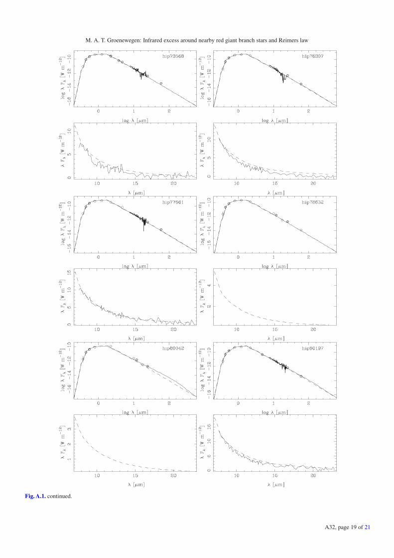
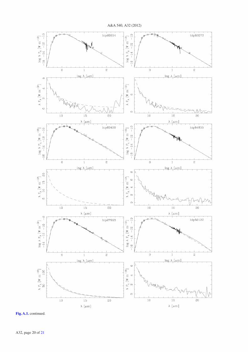
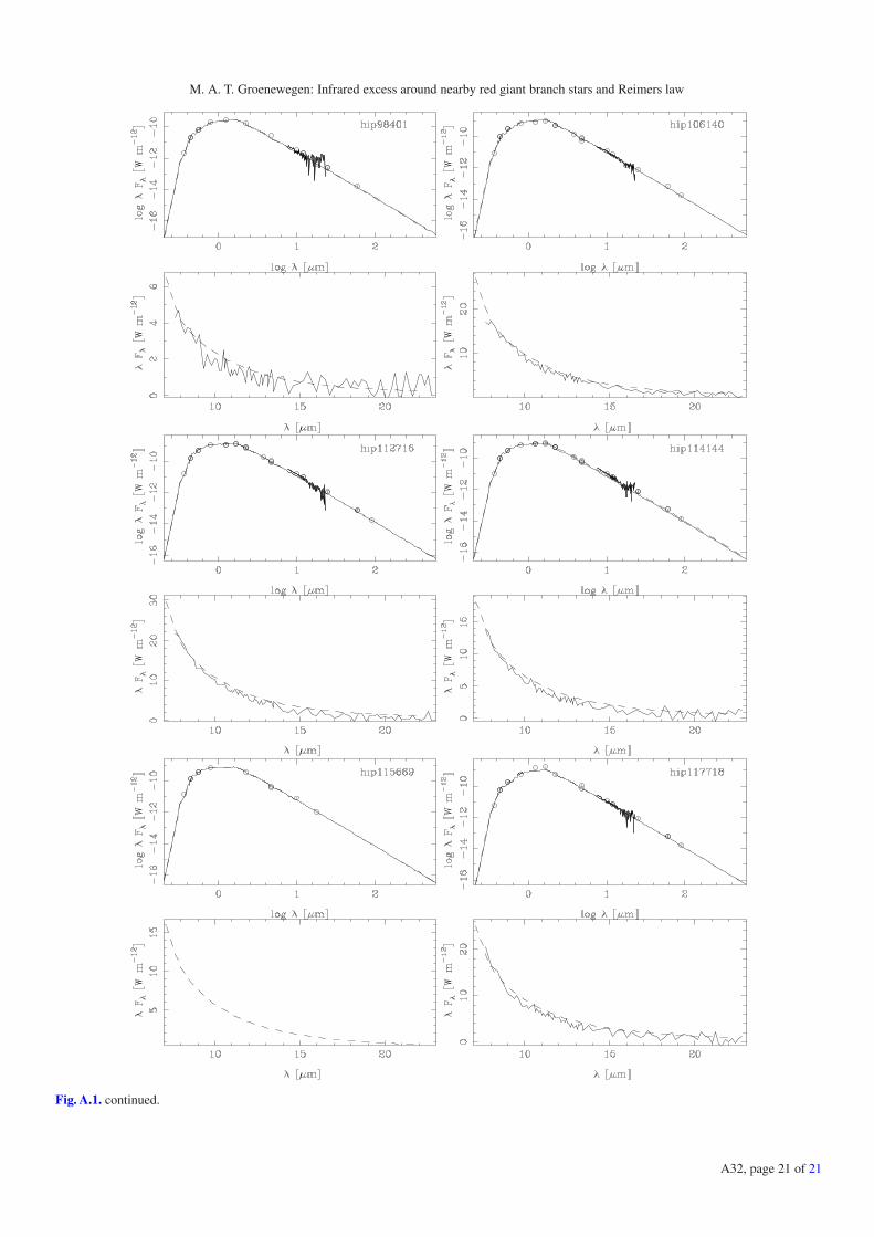
Appendix A: Fits to the SEDs
All fits are shown here.
Fig. A.1. Fits to the SED (top panel) and IRAS LRS spectra (lower panel). In the top panel, the solid line indicates the best fit, the dashed line themodel without mass loss (in many cases the two models overlap and are indistinguishable). The observed photometry is inidicated by the circles,and error bars are also plotted, but typically are much smaller than the symbol size. In the lower panel, the best-fit model is indicated by the dashedline, and the LRS spectrum by the solid line. Sometimes no LRS spectrum was available.


![Far-infrared colours of nearby late-type galaxies in the ...mbaes/MyPapers/Boselli et al...e-mail: [sbianchi;laura]@arcetri.astro.it 9 Astrophysics Group, Imperial College, Blackett](https://static.documents.pub/doc/80x56/6094bb72031fe94e3f2f163b/far-infrared-colours-of-nearby-late-type-galaxies-in-the-mbaesmypapersboselli.jpg)


