32
Ingemar Häggström EISCAT HQ EISCAT Data Analysis and the Madrigal Data Base
Ingemar HäggströmEISCAT HQ
EISCAT Data Analysis and the Madrigal Data Base
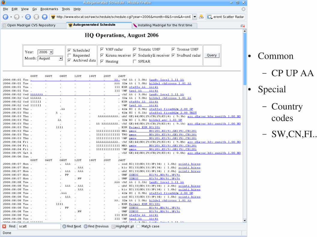
● Common
– CP UP AA● Special
– Country codes
– SW,CN,FI...
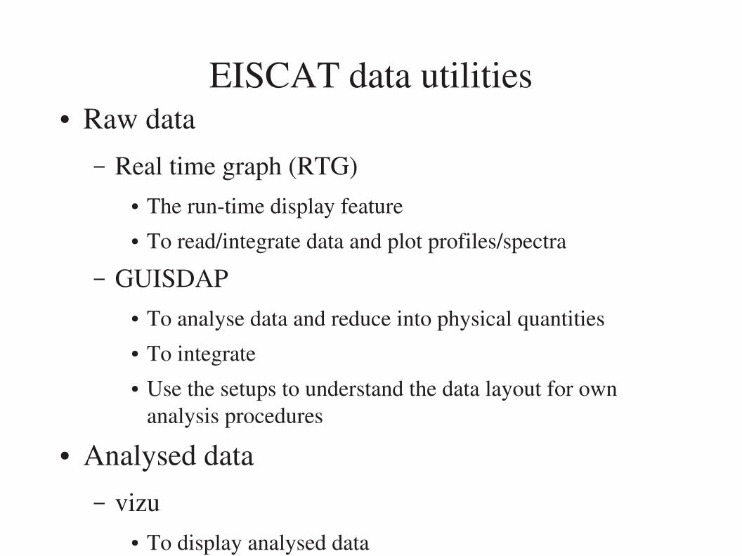
EISCAT data utilities● Raw data
– Real time graph (RTG)● The runtime display feature● To read/integrate data and plot profiles/spectra
– GUISDAP● To analyse data and reduce into physical quantities● To integrate● Use the setups to understand the data layout for own
analysis procedures
● Analysed data– vizu
● To display analysed data
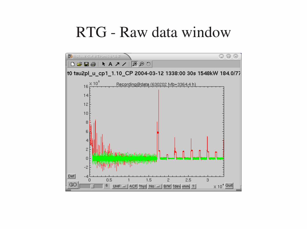
RTG Raw data window
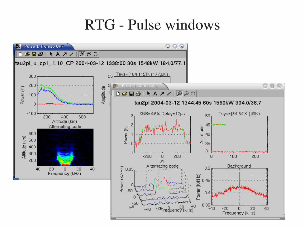
RTG Pulse windows
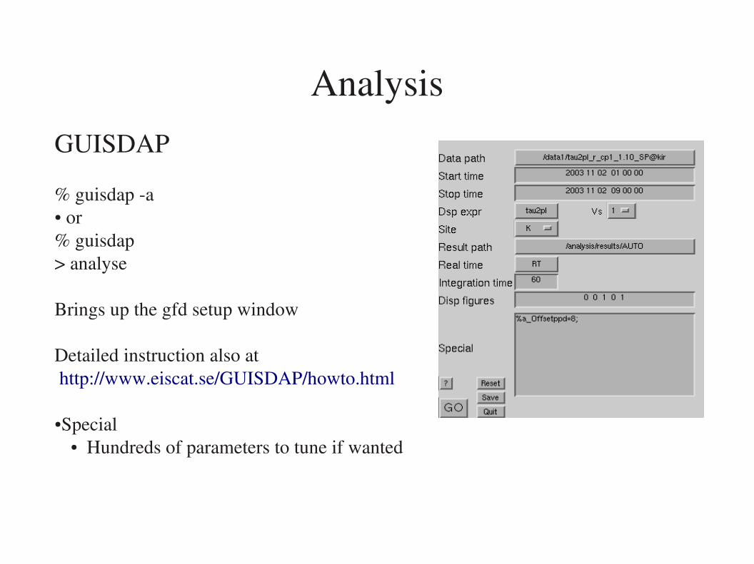
AnalysisGUISDAP
% guisdap a● or% guisdap> analyse
Brings up the gfd setup window
Detailed instruction also at http://www.eiscat.se/GUISDAP/howto.html
●Special● Hundreds of parameters to tune if wanted
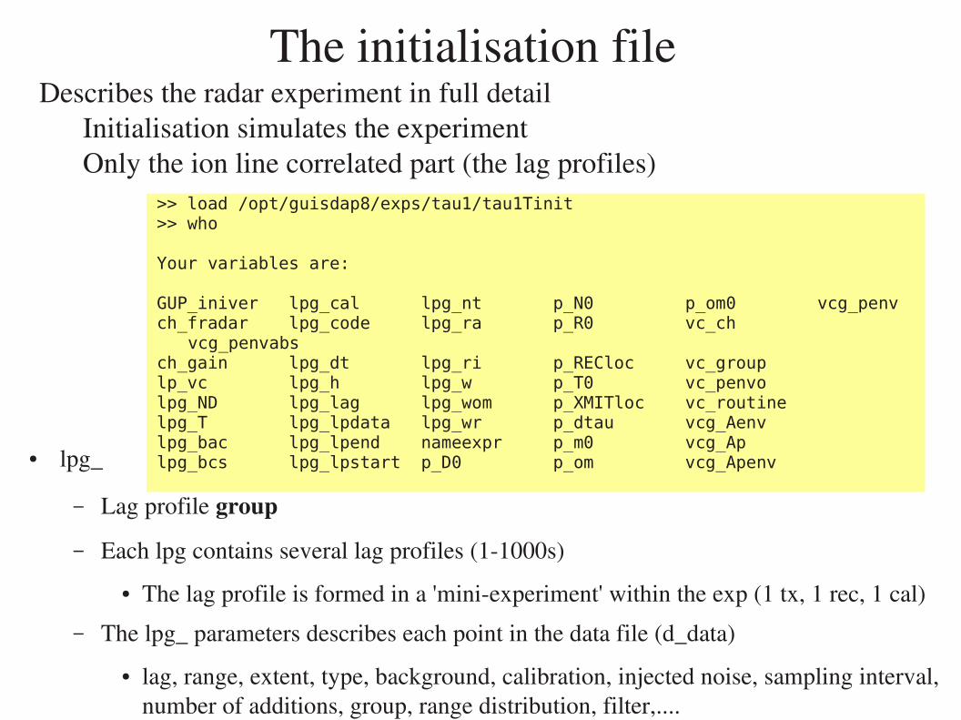
The initialisation file
>> load /opt/guisdap8/exps/tau1/tau1Tinit>> who
Your variables are:
GUP_iniver lpg_cal lpg_nt p_N0 p_om0 vcg_penvch_fradar lpg_code lpg_ra p_R0 vc_ch
vcg_penvabsch_gain lpg_dt lpg_ri p_RECloc vc_grouplp_vc lpg_h lpg_w p_T0 vc_penvolpg_ND lpg_lag lpg_wom p_XMITloc vc_routinelpg_T lpg_lpdata lpg_wr p_dtau vcg_Aenvlpg_bac lpg_lpend nameexpr p_m0 vcg_Aplpg_bcs lpg_lpstart p_D0 p_om vcg_Apenv● lpg_
– Lag profile group
– Each lpg contains several lag profiles (11000s)
● The lag profile is formed in a 'miniexperiment' within the exp (1 tx, 1 rec, 1 cal)
– The lpg_ parameters describes each point in the data file (d_data)
● lag, range, extent, type, background, calibration, injected noise, sampling interval, number of additions, group, range distribution, filter,....
Describes the radar experiment in full detailInitialisation simulates the experimentOnly the ion line correlated part (the lag profiles)
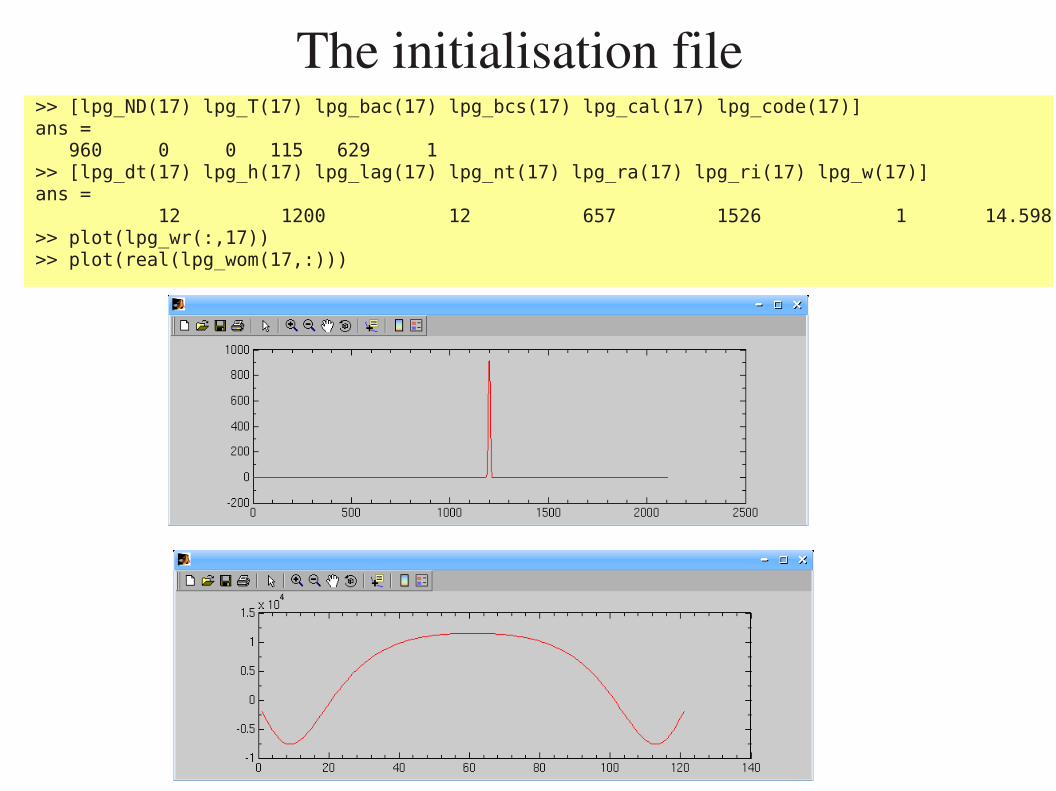
The initialisation file>> [lpg_ND(17) lpg_T(17) lpg_bac(17) lpg_bcs(17) lpg_cal(17) lpg_code(17)]ans = 960 0 0 115 629 1>> [lpg_dt(17) lpg_h(17) lpg_lag(17) lpg_nt(17) lpg_ra(17) lpg_ri(17) lpg_w(17)]ans = 12 1200 12 657 1526 1 14.598>> plot(lpg_wr(:,17))>> plot(real(lpg_wom(17,:)))
The ambiguity vectors
● Spectral ambiguity function– lpg_wom
– Used in fitting process
● Range ambiguity function– lpg_wr
– Space debris detection
– Bistatic volumes
Analysed EISCAT data
● Derived ionospheric parameters– Ne, Ti, Te/Ti, Vi
● Madrigal– NCAR format (madrigal)
● Official product of EISCAT● http://www.eiscat.se/madrigal/cedarFormat.pdf
– HDF5 madrigal vs 3
● Guisdap outputs– Matlab vs 5 (not open)
● r_param
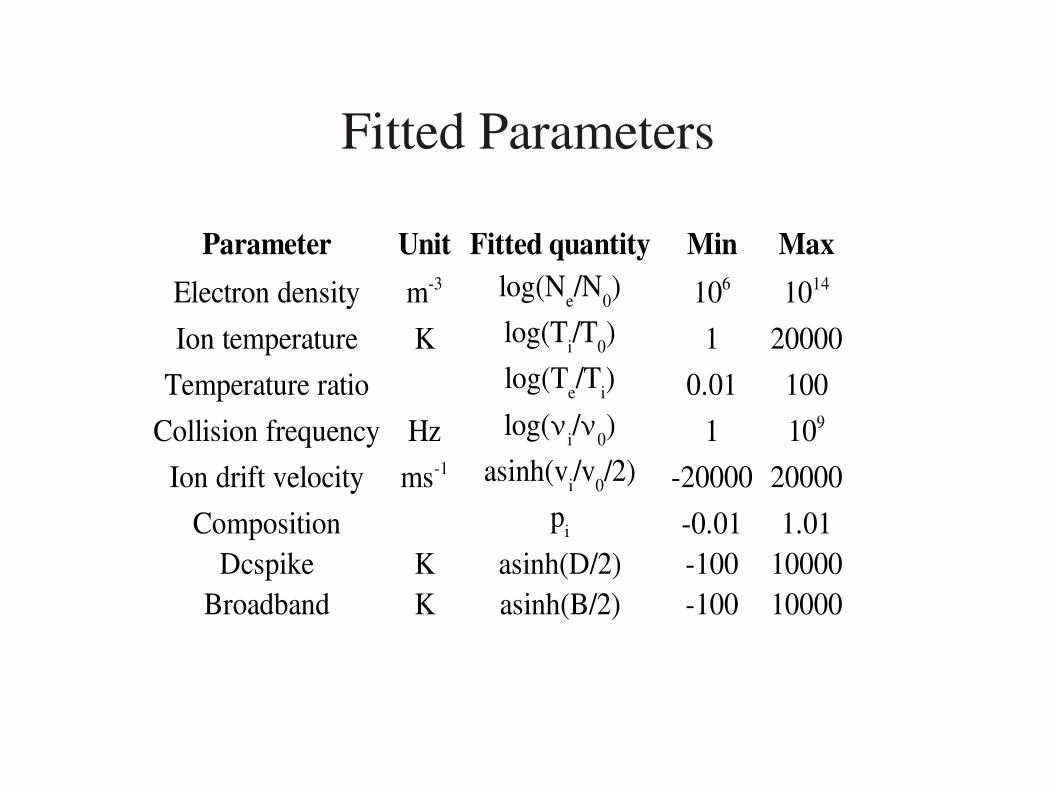
Fitted Parameters
Parameter Unit Fitted quantity Min MaxElectron densityIon temperature K 1 20000
Temperature ratio 0.01 100Collision frequency Hz 1
Ion drift velocity 20000 20000Composition 0.01 1.01
Dcspike K asinh(D/2) 100 10000Broadband K asinh(B/2) 100 10000
m3 log(Ne/N0) 106 1014
log(Ti/T0)log(Te/Ti)log( i/0) 109
ms1 asinh(vi/v0/2)pi
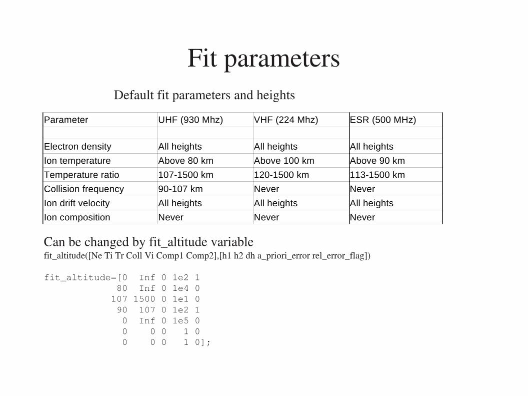
Fit parameters
Parameter UHF (930 Mhz) VHF (224 Mhz) ESR (500 MHz)
Electron density All heights All heights All heights
Ion temperature Above 80 km Above 100 km Above 90 km
Temperature ratio 107-1500 km 120-1500 km 113-1500 km
Collision frequency 90-107 km Never Never
Ion drift velocity All heights All heights All heights
Ion composition Never Never Never
Default fit parameters and heights
Can be changed by fit_altitude variablefit_altitude([Ne Ti Tr Coll Vi Comp1 Comp2],[h1 h2 dh a_priori_error rel_error_flag])
fit_altitude=[0 Inf 0 1e2 1 80 Inf 0 1e4 0 107 1500 0 1e1 0 90 107 0 1e2 1 0 Inf 0 1e5 0 0 0 0 1 0 0 0 0 1 0];
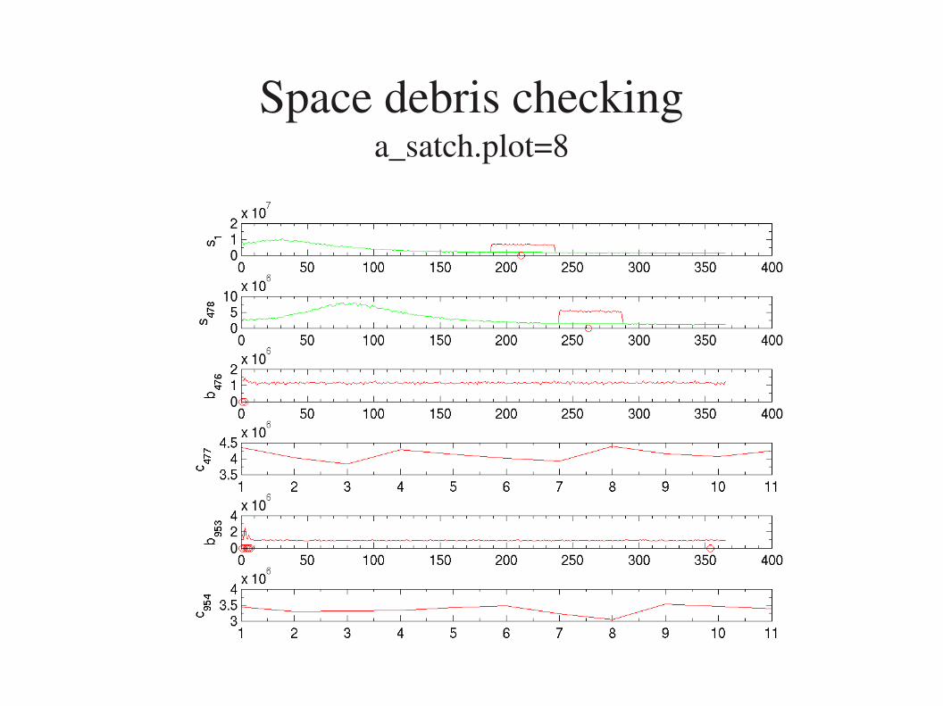
Space debris checkinga_satch.plot=8
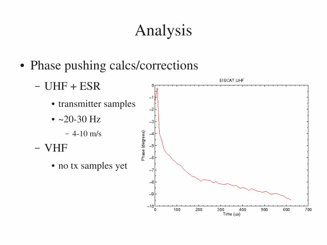
Analysis
● Phase pushing calcs/corrections– UHF + ESR
● transmitter samples● ~2030 Hz
– 410 m/s
– VHF● no tx samples yet
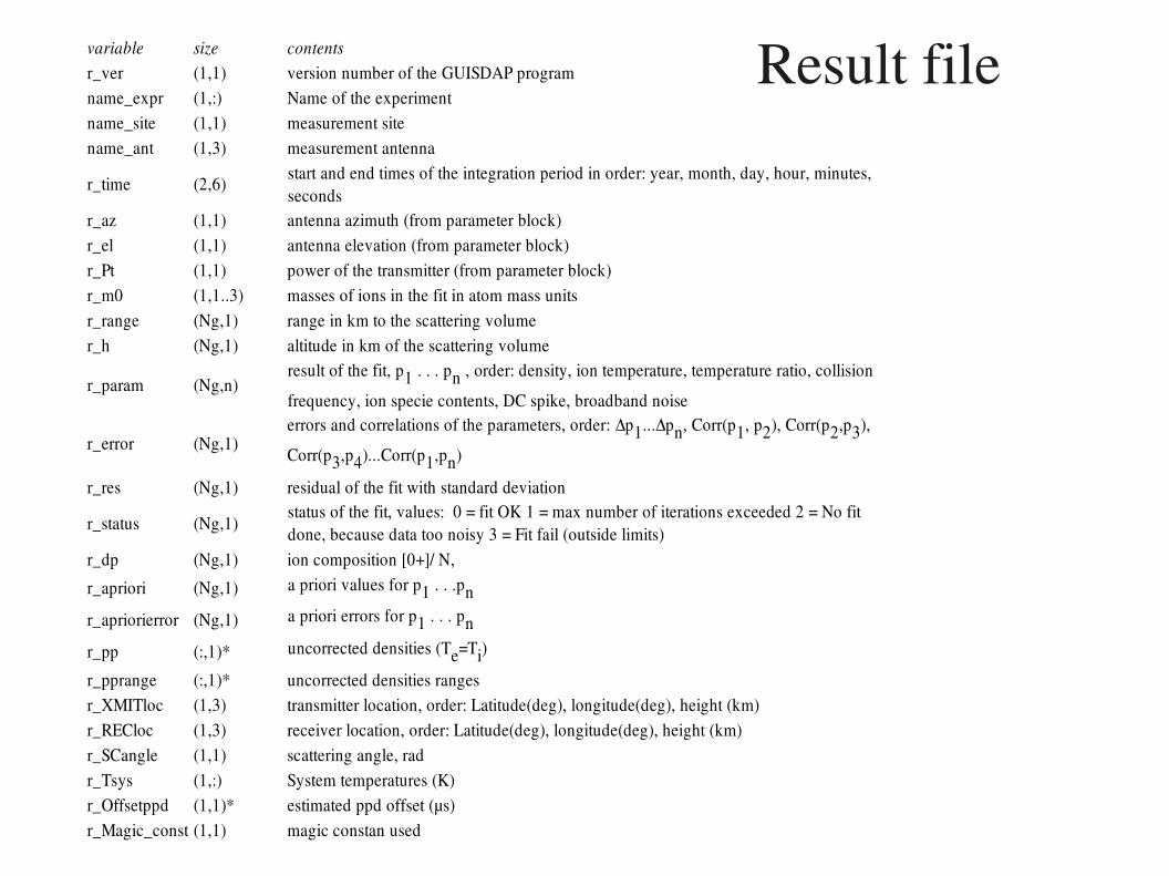
Result filevariable size contentsr_ver (1,1) version number of the GUISDAP programname_expr (1,:) Name of the experimentname_site (1,1) measurement sitename_ant (1,3) measurement antenna
r_time (2,6)
r_az (1,1) antenna azimuth (from parameter block)r_el (1,1) antenna elevation (from parameter block)r_Pt (1,1) power of the transmitter (from parameter block)r_m0 (1,1..3) masses of ions in the fit in atom mass unitsr_range (Ng,1) range in km to the scattering volumer_h (Ng,1) altitude in km of the scattering volume
r_param (Ng,n)
r_error (Ng,1)
r_res (Ng,1) residual of the fit with standard deviation
r_status (Ng,1)
r_dp (Ng,1) ion composition [0+]/ N,
r_apriori (Ng,1)
r_apriorierror (Ng,1)
r_pp (:,1)*
r_pprange (:,1)* uncorrected densities rangesr_XMITloc (1,3) transmitter location, order: Latitude(deg), longitude(deg), height (km)r_RECloc (1,3) receiver location, order: Latitude(deg), longitude(deg), height (km)r_SCangle (1,1) scattering angle, radr_Tsys (1,:) System temperatures (K)r_Offsetppd (1,1)* estimated ppd offset (µs)r_Magic_const (1,1) magic constan used
start and end times of the integration period in order: year, month, day, hour, minutes, seconds
result of the fit, p1 . . . pn , order: density, ion temperature, temperature ratio, collision
frequency, ion specie contents, DC spike, broadband noiseerrors and correlations of the parameters, order: ∆p1...∆pn, Corr(p1, p2), Corr(p2,p3),
Corr(p3,p4)...Corr(p1,pn)
status of the fit, values: 0 = fit OK 1 = max number of iterations exceeded 2 = No fit done, because data too noisy 3 = Fit fail (outside limits)
a priori values for p1 . . .pna priori errors for p1 . . . pnuncorrected densities (Te=Ti)
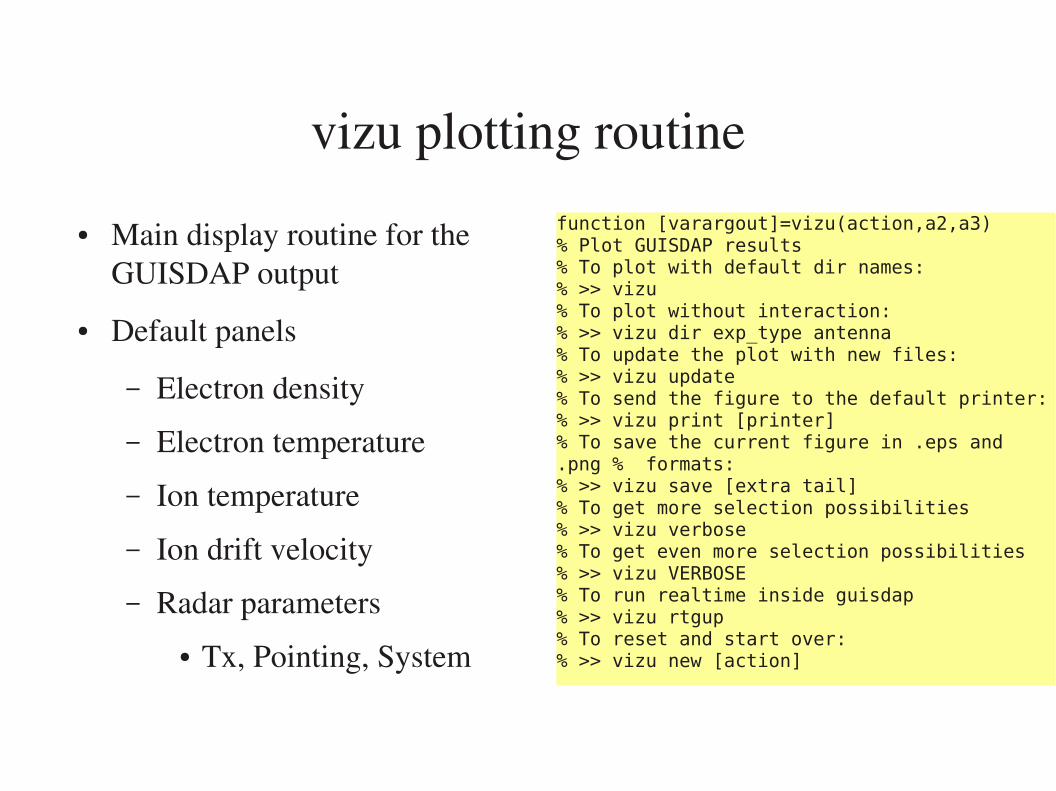
vizu plotting routine
function [varargout]=vizu(action,a2,a3)% Plot GUISDAP results% To plot with default dir names:% >> vizu% To plot without interaction:% >> vizu dir exp_type antenna% To update the plot with new files:% >> vizu update% To send the figure to the default printer:% >> vizu print [printer]% To save the current figure in .eps and .png % formats:% >> vizu save [extra tail]% To get more selection possibilities% >> vizu verbose% To get even more selection possibilities% >> vizu VERBOSE% To run realtime inside guisdap% >> vizu rtgup% To reset and start over:% >> vizu new [action]
● Main display routine for the GUISDAP output
● Default panels
– Electron density
– Electron temperature
– Ion temperature
– Ion drift velocity
– Radar parameters● Tx, Pointing, System
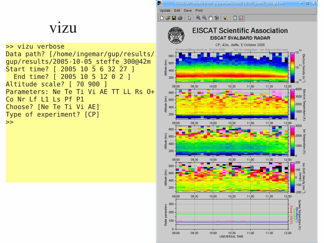
vizu>> vizu verboseData path? [/home/ingemar/gup/results/] gup/results/2005-10-05_steffe_300@42mStart time? [ 2005 10 5 6 32 27 ] End time? [ 2005 10 5 12 0 2 ]Altitude scale? [ 70 900 ]Parameters: Ne Te Ti Vi AE TT LL Rs O+ Co Nr Lf L1 Ls Pf P1Choose? [Ne Te Ti Vi AE]Type of experiment? [CP]>>
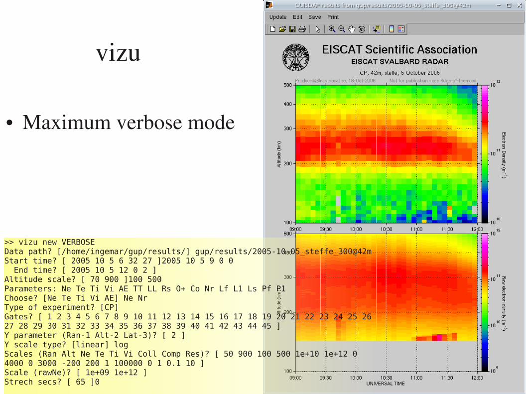
vizu
>> vizu new VERBOSEData path? [/home/ingemar/gup/results/] gup/results/2005-10-05_steffe_300@42mStart time? [ 2005 10 5 6 32 27 ]2005 10 5 9 0 0 End time? [ 2005 10 5 12 0 2 ]Altitude scale? [ 70 900 ]100 500Parameters: Ne Te Ti Vi AE TT LL Rs O+ Co Nr Lf L1 Ls Pf P1Choose? [Ne Te Ti Vi AE] Ne NrType of experiment? [CP]Gates? [ 1 2 3 4 5 6 7 8 9 10 11 12 13 14 15 16 17 18 19 20 21 22 23 24 25 26 27 28 29 30 31 32 33 34 35 36 37 38 39 40 41 42 43 44 45 ]Y parameter (Ran-1 Alt-2 Lat-3)? [ 2 ]Y scale type? [linear] logScales (Ran Alt Ne Te Ti Vi Coll Comp Res)? [ 50 900 100 500 1e+10 1e+12 0 4000 0 3000 -200 200 1 100000 0 1 0.1 10 ]Scale (rawNe)? [ 1e+09 1e+12 ]Strech secs? [ 65 ]0
● Maximum verbose mode
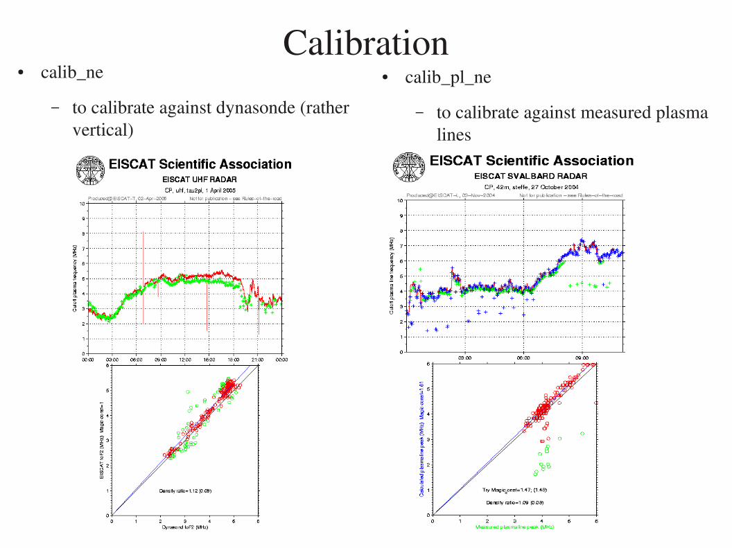
Calibration● calib_ne
– to calibrate against dynasonde (rather vertical)
● calib_pl_ne
– to calibrate against measured plasma lines
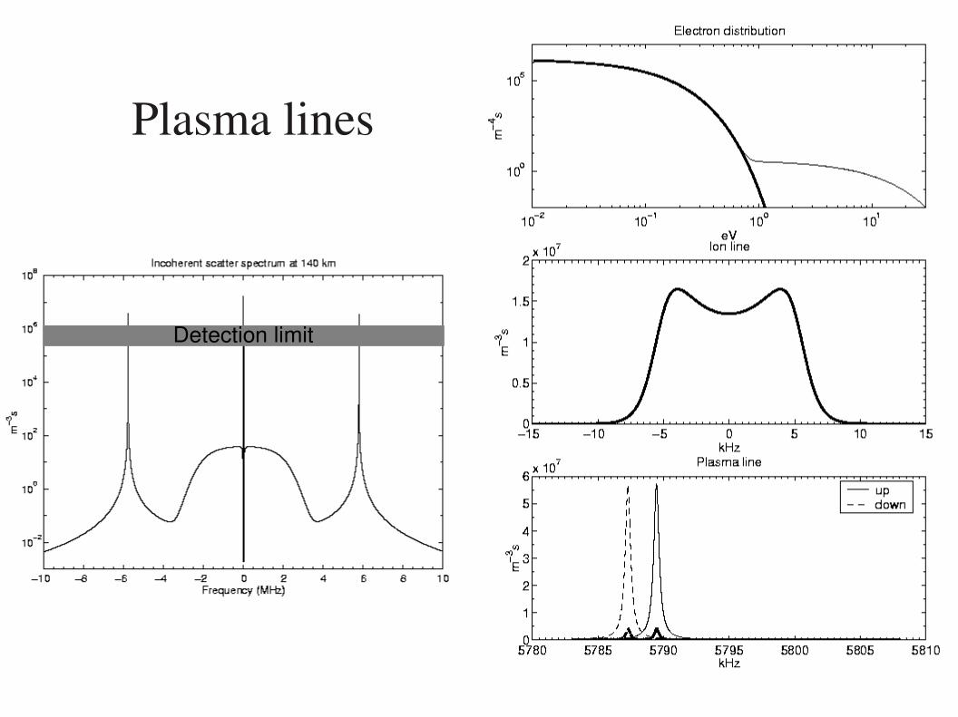
Plasma lines
Detection limit
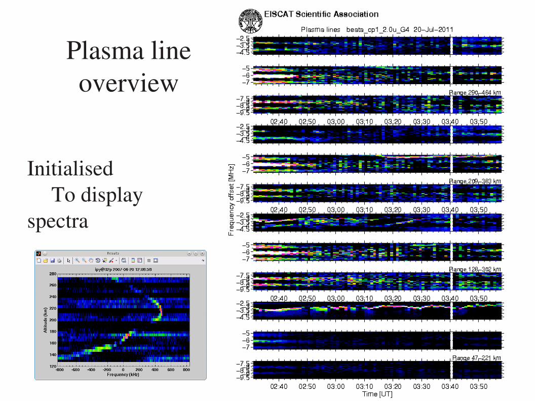
Plasma line overview
InitialisedTo display
spectra
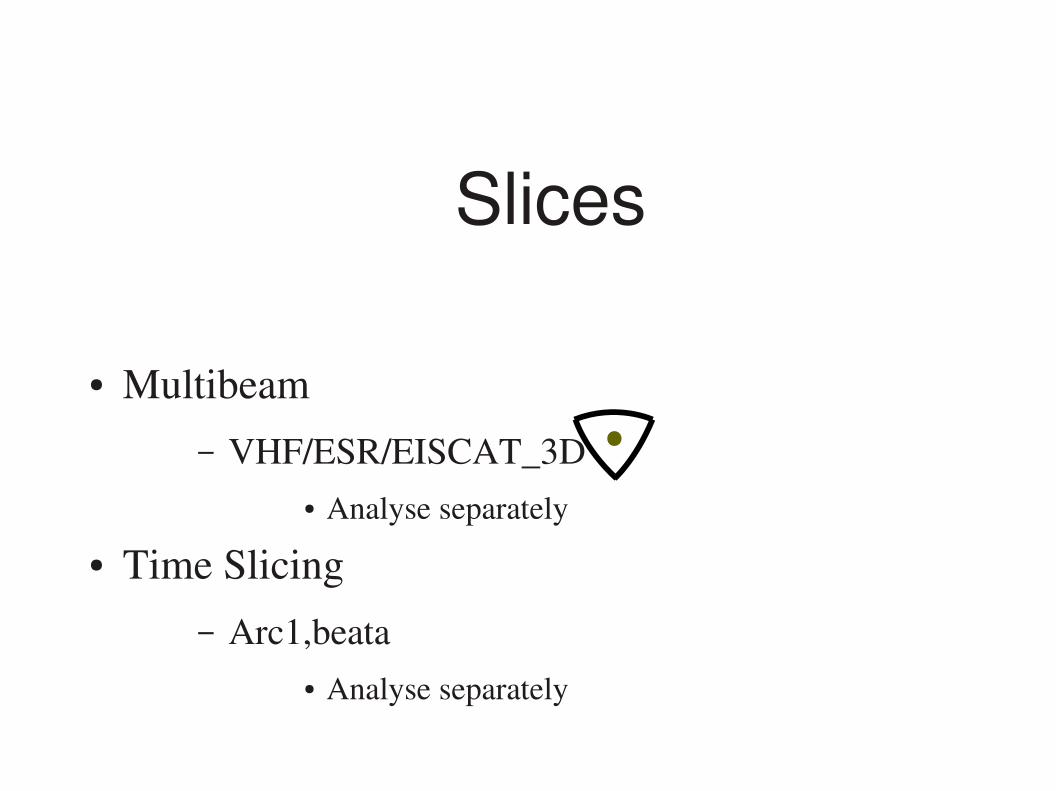
Slices
● Multibeam– VHF/ESR/EISCAT_3D
● Analyse separately
● Time Slicing– Arc1,beata
● Analyse separately
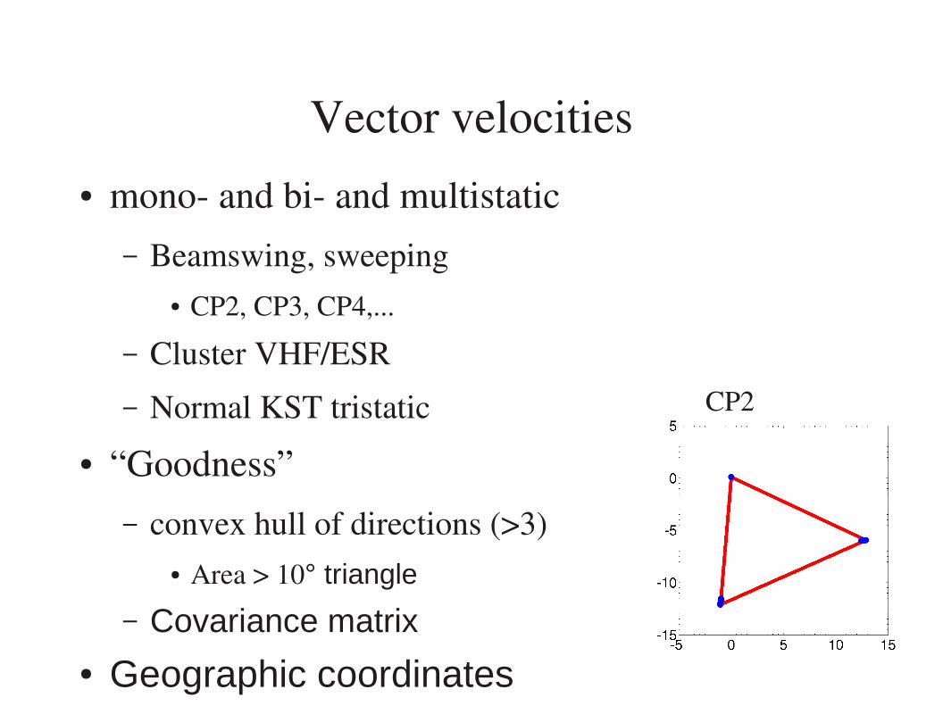
Vector velocities● mono and bi and multistatic
– Beamswing, sweeping● CP2, CP3, CP4,...
– Cluster VHF/ESR
– Normal KST tristatic
● “Goodness”– convex hull of directions (>3)
● Area > 10° triangle
– Covariance matrix
● Geographic coordinates
CP2
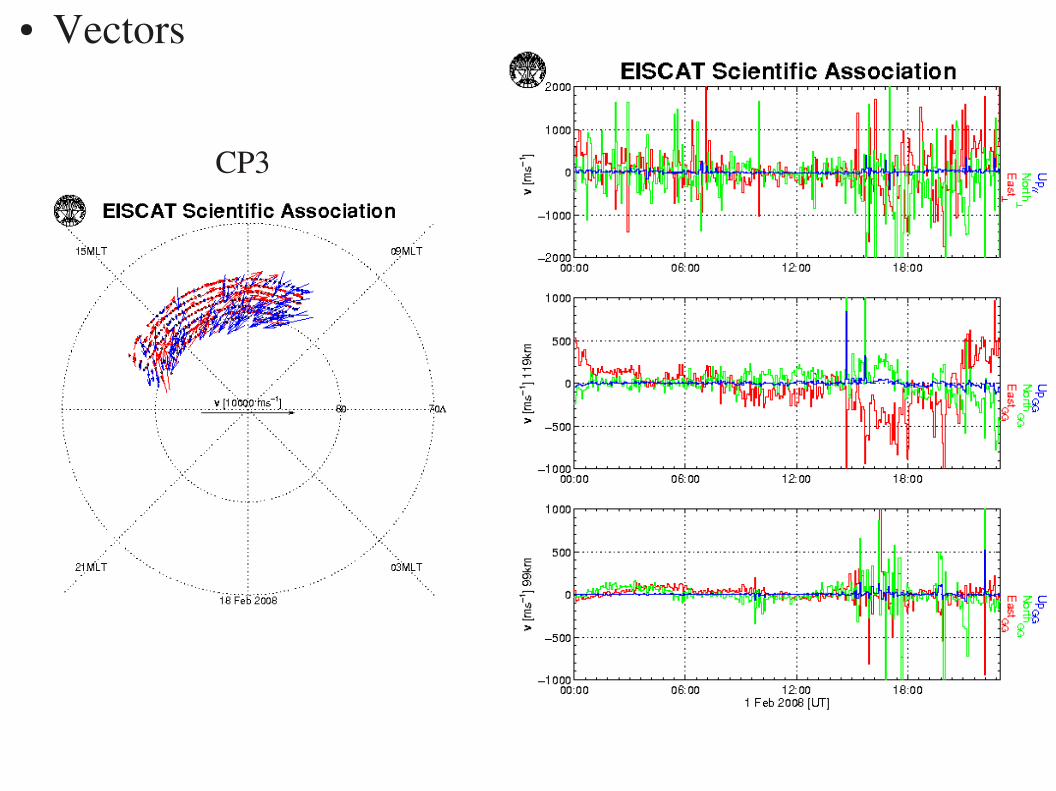
● Vectors
CP3
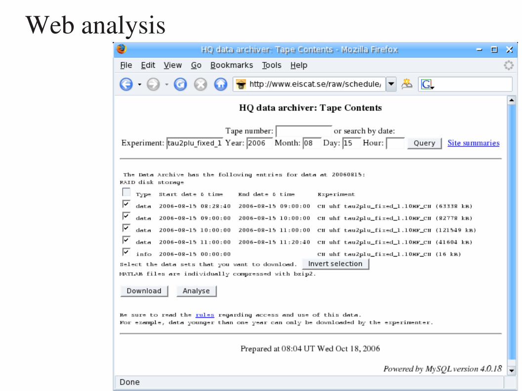
Web analysis
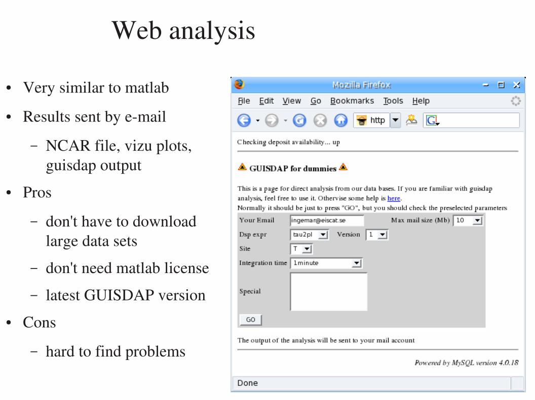
Web analysis
● Very similar to matlab
● Results sent by email
– NCAR file, vizu plots, guisdap output
● Pros
– don't have to download large data sets
– don't need matlab license
– latest GUISDAP version● Cons
– hard to find problems
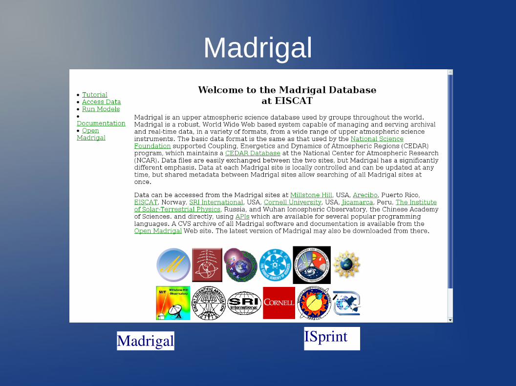
Madrigal
ISprintMadrigal
29
I. Häggström: EISCAT_3D, ISSI Bern 19-23.10.2009
29
Madrigal● Open source
– Python, C, Tcl, Fortran● CVS
– Well-defined format and parameters
– Metadata associated with data files● Allows faster searches of data
– Derivation engine
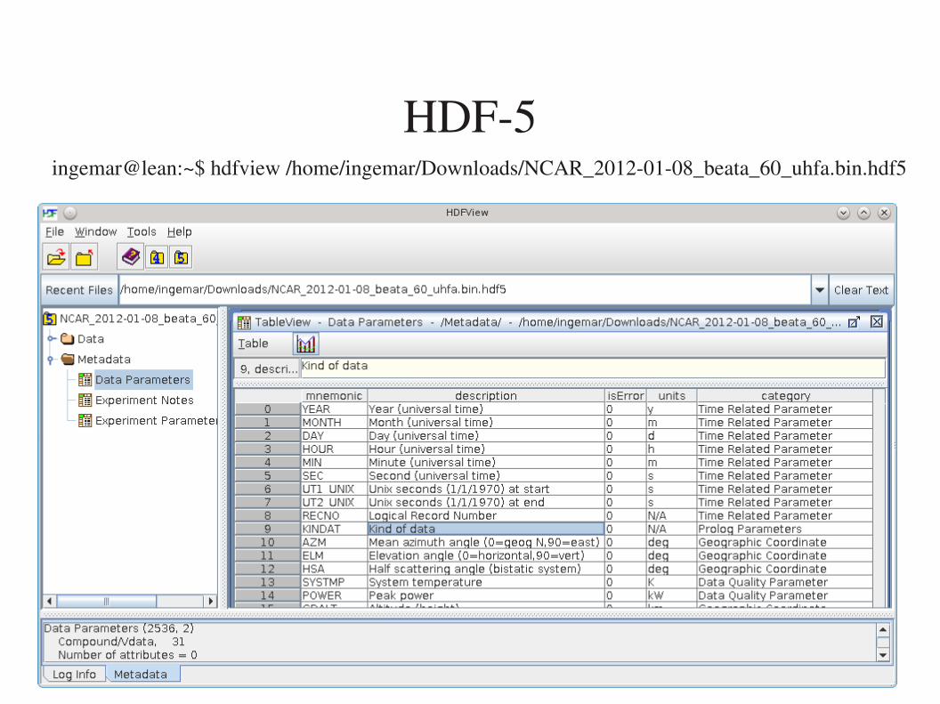
HDF5ingemar@lean:~$ hdfview /home/ingemar/Downloads/NCAR_20120108_beata_60_uhfa.bin.hdf5


