INJECTING CHARTER SCHOOL BEST PRACTICES INTO TRADITIONAL PUBLIC

SCHOOLS:

EVIDENCE FROM FIELD EXPERIMENTS*

Roland G. Fryer, Jr.

Harvard University

April 1, 2014

Abstract

This study examines the impact on student achievement of implementing a bundle of best

practices from high-performing charter schools into low-performing, traditional public schools in

Houston, Texas using a school-level randomized field experiment and quasi-experimental

comparisons. The five practices in the bundle are increased instructional time, more-effective

teachers and administrators, high-dosage tutoring, data-driven instruction, and a culture of high

expectations. The findings show that injecting best practices from charter schools into traditional

Houston public schools significantly increases student math achievement in treated elementary

and secondary schools – by 0.15 to 0.18 standard deviations per year – and has little effect on

reading achievement. Similar bundles of practices are found to significantly raise math

achievement in analyses for public schools in a field experiment in Denver and program in

Chicago. JEL Codes: I21, I24, I28, J24.

*I give special thanks to Terry Grier, Tom Boasberg, and the Houston ISD Foundation’s Apollo 20 oversight

committee whose leadership made this experiment possible. I also thank Richard Barth, James Calaway, Geoffrey

Canada, Tim Daly, Michael Goldstein, Michael Holthouse, and Wendy Kopp for countless hours of advice and

counsel, and my colleagues David Card, Will Dobbie, Michael Greenstone, Lawrence Katz, Steven Levitt, Jesse

Rothstein, Andrei Shleifer, Jörg Spenkuch, Grover Whitehurst, and seminar participants at Barcelona GSE, Brown,

University of California at Berkeley, Harvard, MIT, and NBER Summer Institute for comments and suggestions at

various stages of this project. Brad Allan, Sara D’Alessandro, Matt Davis, Tanaya Devi, Blake Heller, Meghan

Howard Noveck, Lisa Phillips, Sameer Sampat, Rucha Vankudre, and Brecia Young provided truly exceptional

implementation support and research assistance. Financial support from Bank of America, Broad Foundation,

Brown Foundation, Chevron Corporation, the Cullen Foundation, Deloitte, LLP, El Paso Corporation, Fondren

Foundation, Greater Houston Partnership, Houston Endowment, Houston Livestock and Rodeo, J.P. Morgan Chase

Foundation, Linebarger Goggan Blair & Sampson, LLC, Michael Holthouse Foundation for Kids, the Simmons

Foundation, Texas High School Project, and Wells Fargo is gratefully acknowledged. Correspondence can be

addressed to the author by mail: Department of Economics, Harvard University, 1805 Cambridge Street, Cambridge

MA, 02138; or by email: rfryer@fas.harvard.edu. All errors are the sole responsibility of the author. Word

count:15,519.

1

I. INTRODUCTION

New evidence on the efficacy of certain charter schools demonstrates that there exist

combinations of school inputs that can significantly increase the academic achievement of

disadvantaged and minority children (Angrist et al. 2010, 2013; Abdulkadiroglu et al. 2011;

Dobbie and Fryer 2011; Curto and Fryer 2014). But such high-performing charter schools only

serve a small share of U.S. K-12 students. A potential strategy to more broadly improve student

achievement and combat the racial achievement gap is to try to infuse the educational practices

exemplified by the most successful charter schools into traditional public schools. This study

tests whether such practices can improve student achievement within traditional public schools

even in the presence of standard hierarchies and bureaucracies, local politics, school boards, and

collective bargaining agreements.

Starting in the 2010-2011 school year, we1 implemented five best practices of charter

schools described in Dobbie and Fryer (2013) – increased time, better human capital, more

student-level differentiation, frequent use of data to alter the scope and sequence of classroom

instruction, and a culture of high expectations – in twenty of the lowest performing schools

(containing more than 12,000 students) in Houston, Texas.2 To increase time on task, the school

day was lengthened by one hour and the school year was lengthened by ten days in the nine

secondary (middle and high) schools. This was 21 percent more time in school than students in

these schools obtained in the year pre-treatment and roughly the same as achievement-increasing

charter schools in New York City.3 In addition, students were strongly encouraged and even

1 Throughout the text, I depart from custom by using the terms “we”, “our”, and so on. Although this is a sole-

authored work, it took a large team of people to implement the experiments. Using “I” seems disingenuous. 2 These five practices were also implemented in Denver, Colorado starting in the 2011-2012 school year. The

Denver intervention is discussed in Section VI. 3 Using the data set constructed by Dobbie and Fryer (2013), we label a charter school “achievement-increasing” if

its treatment effect on combined math and reading achievement is above the median in the sample, according to their

non-experimental estimates.

2

incentivized to attend classes on Saturday. In the eleven elementary schools, the length of the

day and the year were not changed, but non-instructional activities (e.g. twenty minute bathroom

breaks) were reduced.

In an effort to improve the human capital, nineteen out of twenty principals were

removed and 46 percent of teachers left or were removed before the experiment began. To

enhance student-level differentiation, all fourth, sixth and ninth graders were supplied with a

math tutor and extra reading or math instruction was provided to students in other grades who

had previously performed below grade level. The tutoring model was adapted from the MATCH

school in Boston – a charter school that largely adheres to the methods described in Dobbie and

Fryer (2013). In order to help teachers use interim data on student performance to guide and

inform instructional practice, we required schools to administer interim assessments every three

to four weeks and provided schools with three cumulative benchmark assessments, as well as

assistance in analyzing and presenting student performance data on these assessments. Finally, to

instill a culture of high expectations and college access, we started by setting clear expectations

for school leadership. Schools were provided with a rubric for the school and classroom

environment and were expected to implement school-parent-student contracts. Specific student

performance goals were set for each school and the principal was held accountable and provided

with financial incentives based on these goals.

Such invasive changes were possible, in part, because eleven of the twenty schools (nine

secondary and two elementary) were either “chronically low performing” or on the verge of

being labeled as such and taken over by the state of Texas. Thus, despite our best efforts, random

assignment was not a feasible option for these schools. To round out our sample of twenty

schools and provide a way to choose between alternative quasi-experimental specifications, we

3

randomly selected nine additional elementary schools (vis-à-vis matched-pairs) from eighteen

low – but not chronically low – performing schools. One of the randomly selected treatment

elementary schools closed before the start of the experiment so we had to drop it and its matched

pair from our experimental sample. Thus, our final experimental sample consists of sixteen

schools.

In the sample of sixteen elementary schools in which treatment and control were chosen

by random assignment, providing estimates of the impact of injecting charter school best

practices in traditional public schools is straightforward. In the remaining set of schools, we use

three separate statistical approaches to understand the impact of the intervention. Treatment is

defined as being zoned to attend a treatment school for entering grade levels (e.g. sixth and ninth)

or having attended a treatment school in the pre-treatment year for returning grade levels.

“Comparison school” attendees are all other students in Houston. We begin by using district

administrative data on student characteristics, most importantly previous years’ achievement, to

fit least squares models. We then present two empirical models that instrument for a student’s

attendance in a treatment school with original treatment assignment.4

All statistical approaches lead to the same basic conclusions. Injecting best practices from

charter schools into low performing traditional public schools can significantly increase student

achievement in math and has marginal, if any, effect on English Language Arts (hereafter known

in the text simply as “reading”) achievement. Students in treatment elementary schools gain

around 0.184σ in math per year, relative to comparison samples. Taken at face value, this is

enough to eliminate the racial achievement gap in math in Houston elementary schools in

approximately three years. Students in treatment secondary schools gain 0.146σ per year in math,

4 An earlier version of this paper – Fryer (2011) – also calculated nearest-neighbor matching estimates, which

yielded similar results.

4

decreasing the gap by one-half over the length of the demonstration project. The impacts on

reading for both elementary and secondary schools are small and statistically zero.

In the grade/subject areas in which we implemented all five policies described in Dobbie

and Fryer (2013) – fourth, sixth, and ninth grade math – the increase in student achievement is

substantially larger than the increase in other grades. Relative to students who attended

comparison schools, fourth graders in treatment schools scored 0.331σ (0.104) higher in math,

per year. Similarly, sixth and ninth grade math scores increased 0.608σ (0.093), per year, relative

to students in comparison schools.

Interestingly, both the increase in math and the muted effect for reading are consistent

with the results of achievement-increasing charter schools. Taking the combined treatment

effects at face value, elementary treatment schools in Houston would rank third out of twenty-

seven in math and twelfth out of twenty-seven in reading among NYC charter elementary

schools in the sample analyzed in Dobbie and Fryer (2013).5

We conclude our main statistical analysis by estimating heterogeneous treatment effects

on test scores across a variety of pre-determined subsamples. Most subsamples of the data yield

consistent impacts, though there is evidence that Hispanic students gain significantly more than

black students. In secondary schools, the impact of treatment on black students is 0.065σ (0.043)

and 0.198σ (0.029) for Hispanic students – the p-value on the difference is 0.000. Elementary

schools follow a similar pattern with black students gaining 0.103σ (0.065) and Hispanic

students gaining 0.225σ (0.068) in math.

The above results are robust across identification strategies, alternative student

assessments, and sample attrition. Moreover, an almost identical (non-random assignment) field

5 Dobbie and Fryer (2013) investigate only middle schools, thus, we cannot compare our secondary school results to

their estimates.

5

experiment in Denver, Colorado, and data from a comparable program in Chicago – which uses

four out of the five best practices described above as a core strategy to turn around chronically

low performing schools – yield similar results. Taken together, these data provide evidence that

the best practices in charter schools may be applicable to traditional public schools, and thus, are

general lessons about the educational production function.

The paper is structured as follows: Section II provides background information on the

Houston Independent School District and schools in our sample, as well as details of the field

experiment and implementation. Section III describes our data and research design. Section IV

presents estimates of the impact on state test scores and attendance. Section V provides

robustness checks of our main results. Section VI presents results from a similar field experiment

in Denver and program in Chicago and Section VII concludes. There are three appendices.

Online Appendix A is an implementation guide. Online Appendix B describes how the variables

were constructed in our analysis. Online Appendix C provides some detail on the cost-benefit

calculations presented.

II. BACKGROUND AND PROGRAM DETAILS

II.A. Houston Independent School District

Houston Independent School District (HISD) is the seventh largest school district in the

nation with 203,354 students and 276 schools. Eighty-eight percent of HISD students are black

or Hispanic. Roughly 80 percent of all students are eligible for free or reduced price lunch and

roughly 30 percent of students have limited English proficiency.

Like the vast majority of school districts, Houston is governed by a school board that has

the authority to set a district-wide budget and monitor the district’s finances; adopt a personnel

6

policy for the district (including decisions relating to the termination of employment); enter into

contracts for the district; and establish district-wide policies and annual goals to accomplish the

district’s long-range educational plan, among many other powers and responsibilities. The

Board of Education is comprised of nine trustees elected from separate districts who serve

staggered four-year terms.

II.B. Experimental and Quasi-Experimental Elementary School Sample

In Winter 2011, we ranked all elementary schools in Houston based on their combined

reading and math state test scores in grades three through five and Stanford 10 scores in

Kindergarten through second grade. The two lowest performing elementary schools – Frost

Elementary and Kelso Elementary – were deemed “academically unacceptable” by the state of

Texas and threatened with State takeover. The Houston school district insisted that these schools

be treated. We then took the next eighteen schools (from the bottom) and used a matched-pair

randomization procedure similar to those recommended by Imai, King, and Nall (2009) and

Greevy et al. (2004) to partition schools into treatment and control.6

First, we ordered the full set of eighteen schools by the sum of their mean reading and

math test scores in the previous year. Then we designated every two schools from this ordered

list as a “matched-pair” and randomly drew one member of the matched-pair into the treatment

group and one into the control group. In the summer of 2011, one of the treatment schools was

closed because of low enrollment. We replaced it with its matched-pair. Thus, our final

6 There is an active debate on which randomization procedures have the best properties. Imbens and Abadie (2011)

summarizes a series of claims made in the literature and shows that both stratified randomization and matched-pairs

randomization can increase power in small samples. Simulation evidence presented in Bruhn and McKenzie (2009)

supports these findings, though for large samples there is little gain from different methods of randomization over a

pure single draw. Imai, King and Nall (2009) derive properties of matched-pair cluster randomization estimators and

demonstrate large efficiency gains relative to pure simple cluster randomization.

7

experimental sample consists of eight schools who received treatment and eight who received

control.

In our quasi-experimental specifications, we also include the two elementary schools that

were “academically unacceptable” and the matched-pair for the school that was closed prior to

the start of the experiment for a total of eleven elementary schools that received treatment. The

comparison group is all other elementary students in Houston that have valid test scores in the

relevant years.

II.C. Quasi-Experimental Secondary School Sample

In 2010, four Houston high schools (Sharpstown, Lee, Kashmere, and Jones) labeled

“failing” under Texas Accountability Ratings were declared Texas Title I Priority Schools, the

state-specific categorization for its “chronically low-performing” schools. This meant that these

schools were eligible for federal School Improvement Grant (SIG) funding.7 In addition, four

middle schools were labeled “academically unacceptable” under the Texas Accountability

Ratings in 2009, with a fifth middle school added based on a rating of “academically

unacceptable” in 2010. Unacceptable schools were schools that had proficiency levels below 70

percent in reading, 70 percent in social studies, 70 percent in writing, 55 percent in mathematics,

and 50 percent in science; high schools that had less than a 75 percent completion rate; or middle

schools that had a drop-out rate above two percent.8 Relative to average performance in HISD,

7 These SIG funds could be awarded to any Title I school in improvement, corrective action, or restructuring that

was among the lowest five percent of Title I schools in the state or was a high school with a graduation rate below

60 percent over several years; these are referred to as Tier I schools. Additionally, secondary schools could qualify

for SIG funds if they were eligible for but did not receive Title I, Part A funding and they met the criteria mentioned

above for Tier I schools or if they were in the state's bottom quintile of schools or had not made required Annual

Yearly Progress for two years; these are referred to as Tier II schools. 8 Additionally, schools could obtain a rating of “academically acceptable” by meeting required improvement, even if

they did not reach the listed percentage cut-offs or by reaching the required cut-offs according to the Texas.

8

students in these schools pre-treatment scored 0.414σ lower in math, scored 0.413σ lower in

reading, and were 22 percentage points less likely to graduate.

The difficulty with any quasi-experimental design is constructing valid comparison

schools. In the main analysis, we use the entire HISD sample as a comparison.9

II.D. Program Details

Table I provides a “bird’s eye” view of our field experiments in Houston and Denver as

well as a similar program in Chicago. Online Appendix Table 1 and Online Appendix A, an

implementation guide, provide further details. Fusing the best practices described in Dobbie and

Fryer (2013) with the political realities of Houston, its school board, and other local

considerations, we developed the following five-pronged intervention designed to inject best

practices from charter schools into low performing public schools.

Tenet 1: Extended Learning Time

In elementary schools, we extended the school year by roughly 35 days by “strongly

encouraging” students to attend Saturday classes tailored to each student’s needs. Moreover,

within the school day, we reduced the time spent on non-instructional activities (e.g. eliminating

twenty minute breaks between class periods).

In secondary schools, the school year was extended ten days – from 175 in the pre-

treatment years to 185 for the treatment years. Similar to the elementary schools, students in

secondary schools were strongly encouraged to attend classes on Saturdays. The school day was

extended by one hour each Monday through Thursday.

Projection Measure (TPM). The TPM is based on estimates of how a student or group of students is likely to

perform in the next high-stakes assessment. 9 To check the robustness of this assumption, we also investigate treatment effects using alternative sets of

comparison schools in the Online Appendix.

9

In total, treatment students were in school 1537.5 hours for the year compared to an average of

1272.3 hours in the previous year – an increase of 21 percent. For comparison, the average

charter school in NYC has 1402.2 hours in a school year and the average achievement-increasing

charter school has 1546.0 hours (Dobbie and Fryer 2013). Importantly, because of data

limitations, this does not include instructional time on Saturday. The prevalence of Saturday

school in comparison schools is unknown. The per-pupil marginal cost of the extended day was

approximately $550.

Tenet 2: Human Capital

Leadership Changes

Nineteen out of twenty principals were replaced in treatment schools; compared to

approximately one-third of those in control and comparison schools. To find principals for each

campus, applicants were initially screened based on their past record of achievement in former

positions. Those with a record of increasing student achievement were also given the STAR

Principal Selection Model™ from The Haberman Foundation to assess their values and beliefs in

regards to student achievement. Individuals who passed these initial two screens were

interviewed by the author and the Superintendent of schools to ensure the leaders possessed

characteristics consistent with leaders interviewed in achievement-increasing charter schools.

Initial Staff Departure

Two pieces of data were used to make decisions on which elementary school staff would

remain in treatment schools: value-added data and classroom observations. Value-added data

were available for 137 teachers (roughly 33 percent of all teachers). The HISD employee

charged with managing the principals of treatment schools conducted classroom observations of

10

all teachers in the Winter and Spring of 2011. In total, 38 percent of teachers left or were

removed from the eleven elementary schools.

We used a different approach to remove staff in secondary schools – due solely to the

time available for in-person observations. In 2010, we began with nine secondary schools in late

Spring and the experiment commenced in August – there were three and a half months of

planning, but only one month in which teachers were present in schools. It was not feasible to

observe 562 teachers in their classrooms in twenty days. For the elementary schools, we began

observing teachers in their classrooms almost a year before the experiment started.

Thus given the time constraints, we collected four pieces of data on each teacher in the

nine treatment secondary schools. The data included principal evaluations of all teachers from

the previous principal of each campus (rating them from low performing to highly effective), an

interview to assess whether each teacher’s values and beliefs were consistent with those of

teachers in achievement-increasing charter schools, a peer-rating index, and value-added data, as

measured by SAS EVAAS®, wherever available.10

Value-added data were available for just over

50 percent of middle school teachers in our sample. For high schools, value-added data were

only available at the grade-department level in core subjects.

Online Appendix A provides details on how these data were aggregated to make

decisions on who would be offered the opportunity to remain in treatment schools. In total, 46

percent of teachers (or 453) did not return to treatment schools.11

It is important to note: these

10

Within the teacher interview, each teacher was asked to name other teachers within the school who they thought

to be necessary to a school turnaround effort. From this, we were able to construct an index of a teacher’s value as

perceived by her peers. 11

If one restricts attention to reading and math teachers, teacher departure rates are 60 percent.

11

teachers were not simply reallocated to other district schools; HISD spent over $5 million buying

out teacher contracts.12

Panel A of Figure I compares teacher departure rates in treatment and comparison

schools. Between the 2005-2006 and 2008-2009 school years, teacher departure rates declined

from 28 percent to 18 percent in secondary treatment schools and from 22 percent to 12 percent

in secondary comparison schools. In the summer preceding the treatment year (2010-2011),

teacher departure rates increased slightly at comparison secondary schools to 17 percent, while

52 percent of teachers in treatment secondary schools did not return. To get a sense of how large

this is, consider that this is almost as much turnover as these same schools had experienced

cumulatively in the preceding three years. Elementary schools experienced a similar trend with

declining departure rates until the summer before the treatment year (2011-2012), when there

was a very small increase in departure rates at control schools and a much larger spike in

treatment elementary schools.

Panels B and C of Figure I show differences in value-added of teachers (TVA) on student

achievement for those who remained at treatment elementary and secondary schools,

respectively, versus those who left (for teachers with valid data). The value-added scores have

been standardized to have a mean of zero and a standard deviation of one within subject and

year. Two observations are worth noting. First, in all but one case, teachers who remained in

treatment schools had higher average value-added than those who left. However, aggregately, the

teachers who remained still had lower value-added than the mean teacher in Houston across all

subject areas in elementary schools and two out of five subject areas in secondary schools.

12

One might worry that these teachers simply transferred to comparison schools and that our results are therefore an

artifact of teacher sorting. Two facts argue against this hypothesis. First, only 1.2 percent of teachers in comparison

schools worked in treatment schools in the pre-treatment year. Second, our results are robust to alternative

constructions of comparison schools, including using schools from other large cities across Texas.

12

Second, the change in value-added is not large enough to generate the observed treatment effects.

Taking the increase in value-added from the initial staff turnover at face value and assigning all

new teachers to the mean, the expected increase in test scores is between 0.016σ and 0.025σ in

math and 0.008σ and 0.012σ in reading in secondary schools. In elementary schools, the

anticipated increase in student achievement is between 0.043σ and 0.068σ in math and 0.038σ

and .061σ in reading. Thus, the treatment effects described below are not likely due solely to

reallocation of talented teachers.

Staff Evaluation, and Feedback

One of the most important components of achievement-increasing charter schools is the

feedback given to teachers by supervisors on the quality of their instruction (Dobbie and Fryer

2013). In a typical Houston school, teachers are observed in their classroom three times a year

and provided with written feedback and face-to-face conferences. These observations are an

important part of their yearly evaluation, as part of HISD’s Appraisal and Development Cycle,

which also includes standards on teacher professionalism and multiple measures of student

performance. In treatment schools, teachers received approximately ten times more observations

and feedback. This feedback came in the form of follow-up emails, written notes, and informal

meetings in addition to the formal observation protocol required by the district.13

Staff Development and Training

Each summer, principals coordinated to deliver training to all teachers around the

instructional strategies developed by Doug Lemov of Uncommon Schools, author of Teach Like

a Champion, and Dr. Robert Marzano, a highly regarded expert on curriculum and instruction.

13

Our approach to evaluation and feedback – modeled after achievement-increasing charter schools – is also similar

to the model used in Cincinnati Public Schools (Taylor and Tyler 2011). An important difference is that the Teacher

Evaluation System (TES) implemented in Cincinnati is designed to provide intense evaluation every five years. In

our demonstration project, intense evaluation is done yearly.

13

Moreover, a series of sessions were held on Saturdays throughout the school year designed to

increase the rigor of classroom instruction and address specific topics such as classroom

management, lesson planning, differentiation, and student engagement.

Tenet 3: High-Dosage Tutoring

Many achievement-increasing charter schools provide their students with differentiation

in a variety of ways – some use technology, some reduce class size, while others provide for a

structured system of in-school tutorials. In an ideal world, we would have lengthened the school

day by two hours and used the additional time to provide tutoring in both math and reading for

students in every grade level. This is the model developed by Michael Goldstein at the MATCH

charter school in Boston, Massachusetts.

Due to budget constraints, we were only able to tutor in one grade and one subject per

school. We chose fourth, sixth and ninth grades given the research suggesting that these are

critical growth years (Kurdek and Rodgon 1975; Allensworth and Easton 2005; Anderson 2011),

and we chose math over reading because of the availability of curriculum and knowledge maps

that are more easily communicated to first time tutors.14

Fourth grade students identified as high-need received daily three-on-one tutoring in

math in all treatment elementary schools. Since the school day was not extended in elementary

schools, tutors had to be accommodated within the normal school day. Schools utilized a “pull-

out” model in which identified students were pulled from regular classroom math instruction to

attend tutorials in separate classrooms. Math blocks were extended for tutored grades so that

tutoring did not entirely supplant regular instruction. As a result, non-tutored students worked in

14

Another motivation for this design is that the elementary schools that entered during the second year of

implementation (2011-2012) are not in the feeder patterns of the middle schools. Thus it was important to tutor

students in sixth and ninth grades – school entry grades – in order to ensure that entering students all eventually

received the same complete set of baseline skills and knowledge.

14

smaller ratios with their regular instructor. Some campuses additionally used tutors as “push-in”

support during regular classroom math instruction.

For all sixth and ninth grade students, one class period was devoted to receiving two-on-

one tutoring in math. The total number of hours a student was tutored was approximately 189 for

ninth graders and 215 for sixth graders. All sixth and ninth grade students received a class period

of math tutoring every day, regardless of their previous math performance. The tutorials were a

part of the regular class schedule for students, and students attended these tutorials in separate

classrooms laid out intentionally to support the tutorial program.

There were two important assumptions behind the tutoring model: first, we assumed that

all students in low performing schools could benefit from high-dosage tutoring, either to

remediate deficiencies in students’ math skills or to provide acceleration for students already

performing at or above grade level; second, including all students in a grade in the tutorial

program was thought to reduce potential negative stigma often attached to tutoring programs that

are exclusively used for remediation.

In non-tutored secondary grades – seventh, eighth, tenth, eleventh, and twelfth – students

who tested below grade level received a “double dose” of math or reading in the subject in which

they were the furthest behind. The curriculum for the extra math class was based on the Carnegie

Math program (2010-2011), I Can Learn (2011-2013 middle schools) and ALEKS (2011-2013

high schools).15

Each software program is a full-curriculum, mastery-based platform that allows

students to work at an individualized pace and teachers to be facilitators of learning. Moreover,

each program assesses students frequently and provides reports to principals and teachers on a

weekly basis.

15

See Barrow, Markman, and Rouse (2009) for an independent evaluation of I CAN LEARN software.

15

The curriculum for the extra reading class utilized the READ 180 program. The READ

180 model relies on a very specific classroom instructional model: twenty minutes of whole-

group instruction, an hour of small-group rotations among three stations (instructional software,

small-group instruction, and modeled/independent reading) for twenty minutes each, and ten

minutes of whole-group wrap-up. The program provides specific support for special education

students and students with limited English proficiency. The books used by students in the

modeled/independent reading station are leveled readers that allow students to read age-

appropriate subject matter at their tested lexile level. As with the math curricula, students are

frequently assessed in order to adapt instruction to fit individual needs.

Tenet 4: Data-Driven Instruction

Schools individually set their plans for the use of data to drive student achievement.

Some schools joined a consortium of local high schools and worked within that group to create,

administer, and analyze regular interim assessments that were aligned to the state standards.

Other schools used the interim assessments available through HISD that were to be administered

every three weeks for most grades and subjects.

Additionally, the program team assisted the schools in administering three benchmark

assessments in December, February, and March. These benchmark assessments used released

questions and formats from previous state exams. The program team assisted schools with

collecting the data from these assessments and created reports for the schools designed to

identify the necessary interventions for students and student groups. Based on these assessment

results, teachers were responsible for meeting with students one-on-one to set individual

performance goals for the subsequent benchmark assessments and ultimately for the end-of-year

state exam.

16

Tenet 5: Culture of High Expectations

Of the five policies and procedures changed in treatment schools, the tenet of high

expectations and an achievement-driven culture is the most difficult to quantify. Beyond

hallways festooned with college pennants and decked with the words “No Excuses”, “Whatever

it takes”, and “There are no short-cuts”, there are several indicators that suggest that a change in

culture may have taken place. First, all treatment schools had a clear set of goals and

expectations set by the Superintendent. All teachers in treatment schools were expected to adhere

to a professional dress code. Schools and parents signed “contracts” – similar to those employed

by many charter schools – indicating their mutual agreement to honor the policies and

expectations of treatment schools in order to ensure that students succeed. As in high-performing

charters, the contracts were not meant to be enforced – only to set clear expectations.

Many argue that expectations for student performance and student culture are set, in large

part, by the adults in the school building (Thernstrom and Thernstrom 2003). Recall, all

principals and more than half of the teachers were replaced with individuals who we thought

possessed values and beliefs consistent with an achievement-driven philosophy. Teachers in

treatment schools were interviewed as to their beliefs and attitudes about student achievement

and the role of schools; answers received relatively higher scores if they placed responsibility for

student achievement more on the school and indicated a belief that all students could perform at

high levels.

Panel D of Figure I provides some suggestive evidence that a change in culture may have

taken place in treatment schools. It demonstrates the statistically significant differences in the

likelihood of treatment schools versus comparison schools participating in a number of activities

that support changes in “school culture”. Relative to comparison schools, treatment schools were

17

more likely to employ group work, less likely to be engaged in non-instructional activities, more

likely to have rules, data trackers, and achievement goals posted, and more likely to have

students adhering to uniform policies. These data were gleaned by half-day in-person site visits

to all treatment and comparison schools.

III. DATA AND RESEARCH DESIGN

III.A. Data

We use administrative data provided by the Houston Independent School District (HISD).

The main HISD data file contains student-level administrative data on approximately 200,000

students across the Houston metropolitan area, in a given year. The data include information on

student race, gender, free and reduced-price lunch status, behavior, attendance, and matriculation

with course grades for all students; state math and reading test scores for students in third

through eleventh grades; and Stanford 10 subject scores in math and reading for students in

Kindergarten through tenth grade.16

We have HISD data spanning the 2003-2004 to 2012-2013

school years.

The state math and reading tests, developed by the Texas Education Agency (TEA), are

statewide high-stakes exams conducted in the spring for students in third through eleventh

grade.17

Students in fifth and eighth grades must score proficient or above on both tests to

advance to the next grade, and eleventh graders must achieve proficiency to graduate. Because of

this, students in these grades who do not pass the tests are allowed to retake it approximately one

month after the first administration. We use a student’s first score unless it is missing.18

16

HISD did not administer Stanford 10 assessments to high school students after the 2010-2011 school year. 17

Sample tests can be found at http://www.tea.state.tx.us/student.assessment/released-tests/ . 18

Using their retake scores, when the retake is higher than their first score, does not significantly alter the results.

Results available from the author upon request.

18

The content of the state math assessment is divided among six objectives for students in

grades three through eight and ten objectives for students in grades nine through eleven. Material

in the state reading assessment is divided among four objectives in grades three through eight

and three objectives in grade nine. The ninth grade reading test also includes open-ended written

responses. The state reading assessment covers six objectives for tenth and eleventh grade

students and also includes open-ended questions as well as a written composition section.19

All public school students are required to take the math and reading tests unless they are

medically excused or have a severe disability. Students with moderate disabilities or limited

English proficiency must take both tests, but may be granted special accommodations (additional

time, translation services, alternative assessments, and so on) at the discretion of school or state

administrators. In our analysis, the test scores are normalized (across the school district) to have

a mean of zero and a standard deviation of one for each grade and year.20

We use a parsimonious set of controls to help correct for pre-treatment differences

between students in treatment and comparison schools. The most important controls are reading

and math achievement test scores from the three years prior to the start of the experiment, which

we include in all regressions (unless otherwise noted), and are also referred to throughout the text

as “baseline test scores.” We also include two indicator variables for each baseline test score.

The first takes on the value of one if that test score is a Spanish version test and zero otherwise

and the other takes on the value of one if that test is a Stanford 10 version test (for students who

19

Additional information about Texas state tests is available at http://www.tea.state.tx.us/student.assessment/taks/

and http://www.tea.state.tx.us/student.assessment/staar/. 20

Among students who take a state math or reading test, several different test versions are administered to

accommodate specific needs. These tests are designed for students receiving special education services who would

not be able to meet proficiency on a similar test as their peers. Similarly, TAKS/STAAR-- L is a linguistically

accommodated version of the state mathematics, science and social studies test that provides more linguistic

accommodations than the Spanish versions of these tests. According to TEA, TAKS/STAAR--Modified and

TAKS/STAAR--L are not comparable to the standard version of the test and thus, we did not use them for our main

analysis. We did, however, investigate whether treatment influenced whether or not a student takes a standard or

non-standard test (see Online Appendix Table 2).

19

were in lower elementary grades and thus do not have three years of state test score data) and

zero otherwise.

Other individual-level controls include gender; a mutually exclusive and collectively

exhaustive set of race indicator variables; and indicators for whether a student is eligible for free

or reduced-price lunch or other forms of federal assistance, whether a student receives

accommodations for limited English proficiency, whether a student receives special education

accommodations, or whether a student is enrolled in the district’s gifted and talented program.21

Following the logic in Rothstein (2009), we also include a series of school-level controls

in all quasi-experimental specifications. These include the percentage of the school that is

female, the percentage of the school that is black, the percentage of the school that is Hispanic,

the percentage of the school that is white, the percentage of the school that is eligible for free or

reduced price lunch, the percentage of the school that receives accommodations for limited

English proficiency, the percentage of the school that receives special education

accommodations, the percentage of the school that is enrolled in the gifted and talented program,

and the mean math and reading scores on the state test in the three years prior to treatment. The

demographic controls are constructed by taking the mean of each control in each school existing

in HISD in 2010. The math and reading scores for 2007-2008, 2008-2009, and 2009-2010 are

constructed by taking the mean math and reading scores in each school in the year of interest. If

students are enrolled in a school in 2010-2011, 2011-2012, or 2012-2013 that does not exist in

21

A student is income-eligible for free lunch if her family income is below 130 percent of the federal poverty

guidelines, or categorically eligible if (1) the student’s household receives assistance under the Food Stamp

Program, the Food Distribution Program on Indian Reservations (FDPIR), or the Temporary Assistance for Needy

Families Program (TANF); (2) the student was enrolled in Head Start on the basis of meeting that program’s low-

income criteria; (3) the student is homeless; (4) the student is a migrant child; or (5) the student is identified by the

local education liaison as a runaway child receiving assistance from a program under the Runaway and Homeless

Youth Act. Determination of special education or limited English proficiency status is done by HISD Special

Education Services and the HISD Language Proficiency Assessment Committee.

20

either 2007-2008, 2008-2009, or 2009-2010, they are not included in the calculation of school

averages.

Columns (1) through (6) of Table II display descriptive statistics on individual student

characteristics for both our experimental and quasi-experimental samples in elementary schools.

Of the eleven variables, one is statistically significant in our experimental sample: 14.4 percent

of students in control schools are enrolled in a gifted and talented program compared to 10.9

percent in treatment schools.

Columns (7) through (12) report descriptive statistics for secondary schools as well as the

combined sample of all treatment schools, using the rest of the school district as a comparison. In

stark contrast to our experimental elementary school sample, there are marked differences

between treatment and comparison schools. Students in treatment secondary schools are more

likely to be black, more likely to be economically disadvantaged, less likely to be gifted and

talented and have significantly lower baseline scores.22

This is consistent with treatment

secondary schools being chosen because they were the lowest performing in the district.

III.B. Experimental Specifications

For the sixteen elementary schools for which treatment and control were determined by

random assignment, inference is straightforward. Let Zi indicate whether student i was enrolled

in a school selected for treatment during the pre-treatment year, let Xi denote a vector of control

variables consisting of the demographic variables in Table II, and let ( ) represent a polynomial

including three years of individual test scores in both math and reading prior to the start of

22

Since the raw baseline scores do not account for grade or year, we provide standardized scores to allow for a true

comparison between the two groups.

21

treatment and their squares. All of these variables are measured pre-treatment. Further, let γg

denote a grade-level fixed effect, ηt a time fixed effect, and Ψm a matched-pair fixed effect.

The Intent-to-Treat (ITT) effect, τITT, using the eight treatment and eight control schools

in our experimental sample can be estimated with the following regression model:

(1) Yi, m, g, t = α + τITT ∙ Zi + f (Yi, T-1 , Yi, T-2 , Yi, T-3) + βXi + γg + ηt + Ψm + εi, m, g, t

where T represents the treatment year. Equation (1) identifies the impact of being offered a

chance to attend a treatment school, τITT, where students in the matched-pair schools correspond

to the counterfactual state that would have occurred for the students in treatment schools had

their school not been randomly selected. We focus on a fixed population of students.23

And, only

include students with at least one valid baseline test score.24

A student is considered treated

(resp. control) if they were in a treatment (resp. control) school in the pre-treatment year and not

in an exit grade (e.g. fifth grade). All student mobility after treatment assignment is ignored.

Note: because Equation (1) is estimated on third, fourth, and fifth graders and treatment

assignment was determined in the pre-treatment year, we eliminate the concern of students

selecting into an entry grade (e.g. Kindergarten). The ITT effect is estimated both by year, by

holding t constant, and for the two years combined, by pooling the data.

In any experimental analysis, a potential threat to validity is selection out of sample

(selection into the sample is ruled out due to random assignment). For instance, if schools that

implement best practices of charter schools are more likely to have low performing students exit

23

Online Appendix Table 3 provides the numbers of students in each grade and year in our regressions. 24

Given treatment students were already enrolled in treatment schools in the year pre-treatment, this only eliminates

a small fraction of cases in which students were enrolled but were missing a score. Adding these students into the

regressions and including an indicator for missing baseline test score does not alter the results (see Online Appendix

Table 4).

22

the sample (leave the school district, say), then our estimates will be biased even under random

assignment. We find that 8.0 percent of treatment students are missing a test score relative to 6.6

percent of control students, a difference of 1.4%. Given the small amount of differential selection

relative to the effect sizes, calculating standard bounds leaves the qualitative conclusions

unchanged. This issue is addressed in more detail in Section IV.

Under several assumptions (e.g. that treatment assignment is random, control schools are

not allowed to participate in the program and treatment assignment only affects outcomes

through program participation), we can also estimate the causal impact of attending a treatment

school. This parameter, commonly known as the Local Average Treatment Effect (LATE),

measures the average effect of attending a treatment school on students who attend as a result of

their school being randomly selected (Imbens and Angrist 1994). We estimate two different

LATE parameters through two-stage least squares regressions, using random assignment as an

instrumental variable for the first stage regression. The first LATE parameter uses an indicator

variable, EVER which is equal to one if a student attended a treatment school for at least one day.

More specifically, in the 2012 specification, EVER is equal to one if a student attended a

treatment school in the 2011-2012 school year and zero otherwise and uses test scores from 2012

as an outcome. In the 2013 specification, EVER is equal to one if a student attended a treatment

school for at least one day in 2012 or 2013 and zero otherwise and uses test scores from 2013 as

an outcome. In the pooled specification, EVER is equal to one if a student attended a treatment

school for at least one day in either 2012 or 2013 and zero otherwise and uses both test scores

from both 2012 and 2013 as an outcome. The second stage equation for the two-stage least

squares estimate therefore takes the form:

(2) Yi, m, g, t = α + ΩEVERi, m, g, t + f (Yi, T-1 , Yi, T-2 , Yi, T-3) + βXi + γg + ηt + Ψm + εi, m, g, t

23

and the first stage equation is:

(3) EVERi, m, g, t = α + λZi + f (Yi, T-1 , Yi, T-2 , Yi, T-3) + βXi + γg + ηt + Ψm + εi, m, g, t

where all other variables are defined in the same way as in Equation (1). When Equation (2) is

estimated for one year only, Ω (referred to as 2SLS (Ever) in tables) provides the cumulative

treatment effect after that year. When Equation (2) is estimated across multiple years, as in the

pooled estimates, Ω provides the weighted average of the cumulative effects of attending a

treatment school.

Our second LATE parameter is estimated through a two-stage least squares regression of

student achievement on the intensity of treatment. More precisely, we define TREATED as the

number of years a student is present at a treatment school. The second stage equation for the two-

stage least squares estimate therefore takes the form:

(4) Yi, m, g, t = α + δTREATEDi, m, g, t + f (Yi, T-1 , Yi, T-2 , Yi, T-3) + βXi + γg + ηt + Ψm + εi, m, g, t

The first stage equation is equivalent to Equation (3), but with TREATED as the dependent

variable. In the 2012 specification, TREATED ranges from zero to one and uses test scores from

2012 as an outcome. In the 2013 specification, TREATED ranges from zero to two and uses test

scores from 2013 as an outcome. In the pooled specification, TREATED ranges from zero to two

and uses test scores from both 2012 and 2013 as an outcome. Therefore, δ provides the average

yearly effect of participating in our experiment.

24

III.C. Quasi-Experimental Specifications

In the absence of a randomized experiment in secondary schools, we implement three

quasi-experimental statistical approaches to adjust for pre-intervention differences between

treatment and comparison students. The first and simplest model we estimate is a linear, lagged

dependent variable, specification of the form:

(5) Yi, s, g, t = α + τOLS ∙ Zi + f (Yi, T-1 , Yi, T-2 , Yi, T-3) + βXi + ρXs + ωg + Φt + εi, s, g, t

where, i indexes students, s schools, g grades, and t years. This specification also includes a

vector of school-level controls, Xs, analogous to the individual level demographics listed in Table

II as well as three years of mean school-level test scores.25

To mimic our ITT specification, Zi

takes on the value of one if a student was enrolled in a treatment school in the pre-treatment year

and was not in an exit grade and zero otherwise. This is not applicable to students in entry grades

(e.g. sixth and ninth). In this scenario, we define a student as treated if they are zoned to attend a

treatment school. As before, all student mobility after treatment is assigned is ignored. Thus, our

secondary school sample includes sixth, seventh, eighth, ninth, tenth, and eleventh graders in

2010-2011, seventh, eighth, tenth and eleventh graders in 2011-2012, and eighth and eleventh

graders in 2012-2013.26

Equation (5) is a simple and easily interpretable way to obtain quasi-experimental

estimates of the effect of treatment assignment on student outcomes after each year in the yearly

25

The one exception is that Xs does not have a control for the percentage of students in a school with “other” race

since there were so few of these students in the schools. 26

Results for new cohorts that were excluded from our sample are displayed in Online Appendix Table 5A while

results that use all cohorts in treatment schools (not a fixed sample) are displayed in Online Appendix Table 5B.

25

estimates and the weighted average effect in the pooled estimate. The identification argument is

similar to Dehejia and Wahba (1999).

There are two potential threats to identification: selection into or out of the sample.

Selection into the treatment sample is highly unlikely for students in non-entry grades due to our

definition of treatment. Students would need to change schools months before the experiment

was ever conceived. It is possible for students in entry grades (sixth and ninth), however, to enter

our sample by moving into a treatment enrollment zone when first entering the district in the

treatment year. To minimize this type of selection, we only include students with a least one year

of valid baseline scores.27

It is also possible for students within the district to move into a

treatment enrollment zone, however given Houston’s open enrollment policy, this seems

unlikely. As before, selection out of treatment is more of a concern. Yet, for our secondary

sample, there seems to be little differential selection out of treatment. If anything, students in

treatment schools are slightly more likely to be in the sample.

We also use two instrumental variable strategies analogous to those used on our

experimental sample to try to understand the impact of the experiment on students who actually

attended treatment schools and how the impact varied with intensity. Consistent with prior

literature (e.g. Abdulkadiroglu et al. 2011), we assume that test score gains are a linear function

of school attendance.28

The first stage equations express attendance in a treatment school as a function of an

indicator, Zi, for whether a student is in the treatment group (i.e. enrolled in a treatment school in

the pre-treatment year if in a non-entry grade or zoned to attend a treatment school in the first

27

Results for all students (including those without a valid baseline score) are shown in Online Appendix Table 4 and

are almost identical to our main estimates. 28

If this assumption proves false, our estimates recover a weighted average derivative of the true function. The

expression for the weights is quite complicated without further assumptions, however; see Angrist and Pischke

(2009) for a brief discussion.

26

year of treatment if in an entry grade) and our parsimonious set of controls. As before, EVER is

an indicator variable equal to one if a student attended at least one day in a treatment school up

to the relevant year (or any of the treatment years in the pooled sample) and zero otherwise.

TREATED is a variable that represents the number of years a student spent in a treatment school

and ranges from zero to one in the 2012 specification, zero to two in the 2013 specification and

zero to two in the pooled specification for elementary school students. Similarly, TREATED

ranges from zero to one in the 2011 specification, zero to two in the 2012 specification, zero to

three in the 2013 specification, and zero to three in the pooled specification for secondary

students. The first stage in symbols:

(6) EVERi, s, g, t = α + θZi + f (Yi, T-1 , Yi, T-2 , Yi, T-3) + βXi + ρXs + ωg + Φt + εi, s, g, t

(7) TREATEDi, s, g, t = α + θZi + f (Yi, T-1 , Yi, T-2 , Yi, T-3) + βXi + ρXs + ωg + Φt + εi, s, g, t

The residual of these equations captures other factors that are correlated with enrollment in a

treatment school and may be related to student outcomes. The second stage equations are:

(8) Yi, s, g, t = α + ΩEVERi, s, g, t + f (Yi, T-1 , Yi, T-2 , Yi, T-3) + βXi + ρXs + ωg + Φt + εi, s, g, t

(9) Yi, s, g, t = α + δTREATEDi, s, g, t + f (Yi, T-1 , Yi, T-2 , Yi, T-3) + βXi + ρXs + ωg + Φt + εi, s, g, t

The two LATE parameters that result from second-stage Equations (8) and (9), Ω (referred to as

2SLS (Ever) in tables) and δ (referred to as 2SLS (Years) in tables) give the cumulative

treatment effect after a given year for the single-year estimates and a weighted average of the

27

cumulative treatment effects after each year for the pooled estimates and the average yearly

treatment effect, respectively.

The key identifying assumptions of our approach are that (1) living in a treatment

school’s enrollment zone or attending a treatment school in the pre-treatment year is correlated

with attending a treatment school and (2) the instrument affects student achievement only

through its effect on the probability of attending a treatment school, and not through any other

factor or unobserved characteristics.

The first assumption is testable. Online Appendix Table 6 summarizes our first stage

results. In each specification, living in a treatment zone or previously attending a treatment

school before the announcement of the program strongly predicts attendance in a treatment

school. In the experimental sample, the F-statistic is almost 816 using EVER as the endogenous

variable, and 467 using TREATED as the endogenous variable. In the quasi-experimental

samples, the F-statistic is around 731 in elementary schools and 45 in secondary schools using

EVER as the endogenous variable, and 495 in elementary schools and 37 in secondary schools

using TREATED as the endogenous variable. This suggests that our instrument is strong enough

to allow for valid inference in all of our specifications and samples.

The validity of our second assumption – that the instrument only affects student

outcomes through the probability of attendance – is more difficult to assess. To be violated, the

student’s treatment status must be correlated with outcomes after controlling for the student’s

background characteristics. This assumes, for instance, that parents of children in entry grades do

not selectively move into different zones upon learning of the treatment. For children in non-

entry grades, the assumption is that parents did not have knowledge of the intervention at the

beginning of the previous school year so their school choice decisions could not affect a

28

student’s inclusion in the treatment group. Motivated parents can enroll their children in a

treatment school no matter where they live; the relationship between a treatment zone and

enrollment comes about primarily through the cost of attending, not eligibility. We also assume

that any shocks – for instance, easier tests in the treatment year – affect everyone in treatment

and comparison schools, regardless of address. If there is something that increases achievement

test scores for students in treatment – twenty new community centers with a rigorous after

school program, for example – our second identifying assumption is violated.

In what follows, we show the main results across all three empirical specifications,

broken down by year along with pooled estimates. For clarity of exposition, however, in the text

we concentrate on our 2SLS specification using TREATED as the endogenous variable and

pooled years of data unless otherwise noted.

IV. RESULTS

IV.A. Main Results

Table III presents a series of estimates of the impact of the overall treatment described in

Section I on math and reading achievement state test scores in our experimental sample, using

the specifications described in Section II. These are our cleanest estimates since random

assignment was used. The rows specify the subject tested and each column coincides with a

different empirical model/time period that is being estimated. All results in the ITT and 2SLS

(Ever) columns are average cumulative impacts while the results in the 2SLS (Years) columns

are average yearly impacts. All estimates are presented in standard deviation units. Thus, to get

the total cumulative effect of our intervention, one multiplies the pooled 2SLS (Years) estimate,

or Column (9) by two, since the elementary school intervention lasted for two years. Standard

29

errors, clustered at the school level, are in parentheses below each estimate along with the

number of observations.

Column (3) reports the ITT estimate on the pooled data across years. The impact of being

offered the chance to participate in treatment is 0.135σ (0.051) in math and 0.041σ (0.031) in

reading. The LATE estimate in Column (6), which captures the weighted average cumulative

impact of ever attending a treatment school, is 0.153σ (0.057) and 0.046σ (0.035) in math and

reading, respectively. The LATE estimate in Column (9), which captures the average yearly

impact of the treatment, is 0.112σ (0.042) and 0.034σ (0.026) in math and reading, respectively.

To move from the 2SLS (Years) estimates to the 2SLS (Ever) estimates, we multiply the 2SLS

(Years) by the average time treated conditional on all covariates. For example, for experimental

elementary school students, the average time treated conditional on covariates is 1.37 years (put

differently, 93% of potential treatment time). If we multiply 0.112σ by 1.37, we get 0.153σ. All

three math estimates are statistically significant.29

Table IV presents quasi-experimental estimates for both elementary and secondary

schools. Panel A provides quasi-experimental estimates for our set of treated elementary schools

(the eight that were randomly selected along with the additional three that were treated).30

When

we include all eleven treated elementary schools and all HISD elementary schools as the

comparison group, the estimated treatment effect increases substantially – ranging from 0.202σ

(0.067) for the pooled OLS to 0.184σ (0.060), in the 2SLS (Years) specification.31

The reading

results remain virtually unchanged – estimates are small and marginally significant. Taken at

29

Adjusting the standard errors to account for a small number of clusters – using the methods described in Cameron,

Gelbach, and Miller (2008) – does not alter the statistical significance of the results. 30

Online Appendix Table 7 provides quasi-experimental estimates for our set of experimental schools, which allows

one to compare the experimental and quasi-experimental estimates on a common sample. 31

A few of the elementary school principals were hired in the Spring of the pre-treatment year, potentially

contaminating the baseline test scores. Online Appendix Table 8 attempts to account for this by defining the pre-

treatment year as two years prior to treatment. With this adjustment, the estimated impact of treatment is very

similar, though slightly higher.

30

face value, this implies that the treatment has the potential to close the achievement gap in math

among blacks and Hispanics – relative to whites – in less than three years.

Panel B uses identical quasi-experimental specifications on secondary schools. Results

from the nine secondary schools are similar, though smaller in magnitude. The OLS pooled

estimate is 0.102σ (0.029) in math and -0.008σ (0.016) in reading. The weighted average

cumulative impact of ever attending a treatment school shown in Column (8), is 0.191σ (0.043)

and -0.016σ (0.029) in math and reading, respectively. The average yearly impact of the

treatment in Column (9), is 0.146σ (0.031) in math and -0.012σ (0.022) in reading,

respectively.32

Thus, after three years, students in treatment schools gained around 0.438σ in

math. The achievement gap in math in secondary schools in Houston, in the pre-treatment year,

was 0.8σ, implying treatment could close over half the gap over the course of the experiment.

Another, perhaps simpler, way to look at the data is to graph the distribution of average

test score gains for each school-grade cell, which is depicted in Figure II. We control for

demographic observables by estimating Equation (5) in the final year of treatment, but omitting

the treatment indicator. We then collect the residuals from this equation and average them at the

school-cohort level. The results echo those found in Tables III and IV. In elementary school

math, 13 out of 22 school-grade level cells had positive gains. In secondary math, eight out of

nine had positive gains. Online Appendix Figures 1 show adjusted means graphed from the pre-

treatment year to the present in the experimental elementary school, all elementary school, and

secondary school samples. These were calculated by estimating Equation (5) by year of

treatment but omitting the treatment indicator.33

The figures provide a graphical version of the

32

Online Appendix Tables 9A-9D show results for both elementary and secondary schools broken down by cohort

and year. Estimates are similar to those in our main tables. 33

Online Appendix Figure 2 shows unadjusted means from the pre-treatment year to the present for the same

samples.

31

data in Tables III and IV. For both elementary and secondary schools, significant gains were

made in math in treatment relative to comparison schools. There are negligible effects in reading.

There is another stark observation from Online Appendix Figures 1 – effects seem to

“level off” after year one of treatment. This is similar to the class size literature (Krueger 1999).

Leveling off is one interpretation of the patterns. Another interpretation is that, given how we

have defined treatment, student mobility is ignored and thus students who have moved are still

counted as treated. This explains why the 2SLS (Years) estimate is larger than the ITT. Still

another interpretation concerns the correlation in what the test cover from year to year. If the

tests are either highly correlated or highly complementary then our estimates should be

interpreted as gaining significantly relative to the comparison group and then maintaining that

advantage over the treatment years. If, on the other hand, the tests are assessing very different

skills and there is little complementarity across years, then the results imply that treatment

students are seemingly outperforming the comparison student every year by a constant amount.

A quite conservative form of inference is to run school-level regressions of the impact of

treatment on school-level average test scores. We run both OLS and difference-in-differences

(DD) specifications. Estimates for these specifications are displayed in Online Appendix Table

10. The point estimates using the difference in differences specification are strikingly consistent

in math [0.173σ (0.046)] and reading [0.089σ (0.039)]. Both OLS and DD estimates are

statistically significant.

IV.B. High-Dosage Tutoring

Due to budget constraints, all five tenets described in Dobbie and Fryer (2013) were only

implemented in three grade/subject areas: fourth grade math, sixth grade math, and ninth grade

32

math. In the other grade/subject areas, computerized curriculum was used to individualize

instruction. This provides an opportunity to estimate the marginal impact of the most expensive

element of treatment. If small-group, high-dosage tutoring yields significantly larger increases in

student achievement, then perhaps the costs are justified. If, on the other hand, the correlates in

Dobbie and Fryer (2013) were proxies for individualization that can be imitated with technology,

then the potential for scale is greater, due to lower marginal costs.

Table V estimates the impact of treatment with tutoring relative to comparison school

attendees. Students in secondary schools who received tutoring performed significantly better

than their non-tutored peers in treatment schools. In secondary schools, students who received

tutoring had average yearly math gains of 0.608σ (0.093). Compared to other students in

treatment schools, this is a difference of around 0.400σ. The difference has a p-value of 0.000. In

other words, students who received tutoring in secondary schools outperformed their peers by

over 200 percent. The differences between tutored and non-tutored students in elementary

schools were less pronounced. This could be due to the fact that we are tutoring in higher ratios

in elementary versus secondary school or that elementary students are not sufficiently behind to

take advantage of intense tutoring. Arguing for the latter, the tutoring model was most effective

among high school students.

Let us put the magnitude of these estimates in perspective. Jacob and Ludwig (2008), in a

survey of programs and policies designed to increase achievement among poor children, report

that only three reforms pass a simple cost-benefit analysis: lowering class size, teacher bonuses

for teaching in hard-to-staff schools, and early childhood programs. The effect of lowering class

size from 24 to 16 students per teacher is approximately 0.22σ over three years on combined

math and reading scores (Krueger 1999). The effect of Teach for America, one attempt to bring

33

more skilled teachers into poor performing schools, is 0.15σ in math and 0.03σ in reading

(Decker, Mayer, and Glazerman 2004). The effect of Head Start is 0.147σ (0.103) in applied

problems and 0.319σ (0.147) in letter identification on the Woodcock-Johnson exam, but the

effects on test scores fade in elementary school (Currie and Thomas 1995; Ludwig and Phillips

2008).

All these effect sizes are a fraction of the impact of the treatment that includes tutoring.

The effects closest to the ones reported here are from a series of papers on achievement-

increasing charter schools in which the impacts range from 0.229σ to 0.364σ in math and 0.120σ

to 0.265σ in reading (Angrist et al. 2010, Abdulkadiroglu et al. 2011, Curto and Fryer 2014).

Taking the combined treatment effects at face value, elementary treatment schools in Houston

would rank third out of twenty-seven in math and twelfth out of twenty-seven in reading among

NYC charter elementary schools in the sample analyzed in Dobbie and Fryer (2013).

IV.C. Heterogeneous Treatment Effects

Table VI explores the heterogeneity of our treatment effects across a variety of

subsamples of the data and reports p-values on the difference in reported treatment effects. The

coefficient estimates are from the 2SLS (Years) specification.

Most subsamples of the data yield consistent impacts, though there is evidence that

Hispanic students gained significantly more than black students. In secondary schools, the

impact of treatment on black students is 0.065σ (0.043) and 0.198σ (0.029) for Hispanic students

– the p-value on the difference is 0.000. Elementary schools follow a similar pattern with black

students gaining 0.103σ (0.065) and Hispanic students gaining 0.225σ (0.068) in math.

Additional subsample results are presented in Online Appendix Table 11.

34

IV.D. Attendance

We next consider the effects of treatment on attendance rates. Online Appendix Table 12

demonstrates that all elementary specifications yield small and insignificant impacts on

attendance. This is potentially due to the high baseline attendance rate in Houston elementary

schools (97 percent). In secondary schools, however, the treatment effect is 0.672 (0.251)

percentage points per year – around two percentage points in total over the length of the

demonstration project.

V. ROBUSTNESS CHECKS

In this section, we explore the extent to which the test score results are robust to a simple

falsification test, alternative achievement scores, and sample attrition.34

In all cases, our main

results are qualitatively unchanged.

V.A. Falsification Tests

Following the logic of Rothstein (2010), we perform a partial falsification test by

estimating the impact of attending our treatment schools in the pre-treatment year. We estimate

our quasi-experimental specifications during the 2008-09 school year – two years before the

intervention began. If our identification assumptions are valid, we would expect these estimates

to be statistically zero. Unfortunately, the reverse is not necessarily true. If the estimates are

statistically zero, our research design may still be invalid.

34

We also performed three additional robustness checks. Online Appendix Table 13 uses alternative constructions

of comparison groups to estimate the effect of treatment while an earlier version of the paper shows the results from

four statistical tests of cheating gleaned from Jacob and Levitt (2003) as well from alternative specifications. For

details, see Fryer (2011).

35

Online Appendix Table 14 presents the results of this exercise. The 2SLS estimates show

zero impacts as expected in both math and reading, although the OLS specification does have a

treatment effect of 0.045σ (0.021) in reading. However, since our effects are in math, this does

not provide any evidence that treatment schools have positive effects without the intervention.

We also conduct a similar exercise to explore whether mean reversion might explain our

secondary school results. Since the nine treatment secondary schools were chosen based on

several years of poor performance, one might expect some reversion to the mean. We therefore

selected the nine lowest-performing schools based on 2007-08 state tests and calculated their

treatment effects in 2008-09. The results in Online Appendix Table 15 show no evidence of

significant mean reversion. Online Appendix Figures 3A and 3B present these results graphically

for additional cohorts of data.

V.B. Alternative “Low Stakes” Test Scores

Some argue that improvements on state exams may be driven by test-specific preparatory

activities at the expense of more general learning. Jacob (2005), for example, finds evidence that

the introduction of accountability programs increases high-stakes test scores without increasing

scores on low-stakes tests, most likely through increases in test-specific skills and student effort.

It is important to know whether the results presented above are being driven by actual gains in

general knowledge or whether the improvements are only relevant to the high-stakes state exams.

To provide some evidence on this question, we present data from the Stanford 10.

Houston is one of a handful of cities that voluntarily administers a nationally normed test for

which teachers and principals are not held accountable – decreasing the incentive to teach to the

test or engage in other forms of manipulation. The math and reading tests are aligned with

36

standards set by the National Council of Teachers of Mathematics and the National Council of

Teachers of Reading, respectively.35

Table VII presents estimates of treatment on Stanford 10 math and reading scores. As in

our state test results, there are large and statistically significant effects in math and insignificant

results in reading. Panel A displays results for the experimental sample. The average yearly

estimate in math is 0.109σ (0.055) and the estimate in reading is 0.045σ (0.034); both are similar

to the equivalent estimate on state test scores though a bit smaller. Panel B provides treatment

effects for our quasi-experimental sample. The average yearly estimates for elementary schools

are 0.114σ (0.052) in math and 0.039σ (0.035) in reading. The average yearly estimates for

secondary schools are 0.062σ (0.031) in math and 0.002σ (0.021) in reading. Although smaller in

magnitude, these estimates are similar to the estimates in Table IV.

V.C. Attrition

The estimates thus far use students who are in the treatment or comparison sample, and

for whom we have pre-treatment year test scores. If treatment and comparison schools have

different rates of selection into this sample, our results may be biased. Removing teachers and

nineteen principals was not a process that went unnoticed on local news or in print media. It is

plausible that parents were aware of the major changes and opted to move their families to

another attendance zone within HISD, a private school, or a well-known charter school like KIPP

or YES. In the latter two cases, the student’s test scores will be missing. Our IV strategy does not

account for that type of selective attrition.

35

Math tests include content testing number sense, pattern recognition, algebra, geometry, and probability and

statistics, depending on the grade level. Reading tests include age-appropriate questions measuring reading ability,

vocabulary, and comprehension. More information can be found at

http://www.pearsonassessments.com/HAIWEB/Cultures/en-us/Productdetail.htm?Pid=SAT10C.

37

As mentioned earlier, not all students took the standard math and reading tests. Some

students took the linguistically accommodated versions (TAKS/STAAR L), some took tests with

other accommodations (Modified) and some took tests that were above their grade level. It is

also possible that our program pushed students into taking non-standard versions of the state test

and that this is biasing our estimates.

A simple test for this is to investigate the impact of treatment on the probability of

entering our analysis sample and on taking non-standard tests. As Online Appendix Table 2

shows, students in our experimental elementary sample are 1.4 percent more likely to be missing

a test score, equally likely to take an advanced or modified test, and 0.9 percent less likely to

have taken the linguistically accommodated (L) version of the test. Trimming the experimental

sample by dropping the 1.4 percent of the treatment group with the highest gains over previous

year test scores does systematically alter the results (see Lee 2009). Among secondary schools,

students in treatment are less likely to be missing a test score and equally likely to have taken an

advanced or modified test.

VI. FURTHER EVIDENCE

VI.A. Denver Public Schools

Denver Public Schools (DPS) is the largest school district in Colorado and the thirty-

ninth largest district in the country with 84,424 students and 172 schools. Seventy-two percent of

DPS students are black or Hispanic and approximately 72 percent of all students are eligible for

free or reduced price lunch. Denver, like Houston, is governed by a Board of Education

comprised of seven members elected from separate political districts who serve staggered four-

year terms but, in contrast to Houston, has a particularly strong teacher’s union.

38

In 2011-2012, seven schools in the Far Northeast Region of Denver were selected to

participate in a five-pronged field experiment modeled after the intervention in Houston. In these

schools, new principals were selected and approximately 95 percent of teachers were replaced,

260 instructional hours were added to the school year – over 30 days – through more minutes in

each day and more days per year, interim assessments were administered every six to eight

weeks and a “no-excuses” culture was introduced within the first week of the year. Additionally,

fourth, sixth and ninth graders received math tutoring in 1:3 ratios in elementary schools and 1:2

ratios in secondary schools.

There are four potentially important differences between the Houston and Denver

treatments. First, Denver schools are in a feeder pattern in close geographic proximity to each

other. Some argue that this is important for sustainability. Second, all teachers (tenured and

untenured) were required to reapply for their jobs if they wanted to continue teaching in the

school. This resulted in the high turnover rates reported above. Third, because of a law in

Colorado that provides schools with the opportunity to seek autonomy from district policies

(including union contracts) and to bring more decision making to the campus level – labeled the

Innovation Schools Act – all treatment schools have increased autonomy that provides flexibility

in school scheduling, hiring decisions, rewarding excellence in instruction, and removing

ineffective teachers. Fourth, the Denver intervention used a combination of strategies, including:

phasing out and restarting traditional schools, turning around traditional schools (the strategy

used in Houston), and replacing schools with charter schools (a strategy widely implemented in

places like New York). We only analyze the seven schools that were traditional district schools.

The Far Northeast Region, where all treatment schools are located, has a significantly

higher proportion of black and free or reduced-price lunch students when compared with the rest

39

of DPS. Online Appendix Table 16 shows summary statistics for the seven schools in the field

experiment, as well as the other schools in the Far Northeast Region and all other schools in

Denver for students in third, fourth, sixth, and ninth grades (the tested grades in the sample).

Compared to students in other Denver schools, students in treatment schools are significantly

more likely to be black, free lunch eligible, and have lower baseline scores. The comparison

sample for our analysis includes all students in Denver Public Schools in the same grades as the

treatment grades.

To obtain treatment effects for our field experiment in Denver, we estimate the following

equation:

(10) Yi, g, t = α + τOLS ∙ Zi + f(Yi, T-1 , Yi, T-2 ) + βXi + ωg + Φt + εi, g, t

where Zi is an indicator equal to one if the first school in which student i enrolls in 2011-2012 is

a treatment school and zero otherwise, Xi denotes a vector of control variables consisting of the

demographic variables in Online Appendix Table 16, and ( ) represents a polynomial including

two years of individual test scores in both math and reading prior to the start of treatment and

their squares. All of these variables are measured pre-treatment. Additionally, ωg denotes a

grade-level fixed effect, and Φt a time fixed effect. Thus, τOLS gives an estimate of the

cumulative effect of being assigned to treatment after year t in the yearly estimates and the

weighted average of cumulative effects in each year in the pooled estimate.

Estimates from Equation (10) are presented in Table VIII. The average effect of being

enrolled in a treatment school in Denver in the pooled estimate is 0.172σ (0.065) and 0.076σ

(0.052) in reading. These numbers are remarkably similar to the results in Houston.

40

VI.B. Chicago

Chicago Public Schools (CPS) is the fourth largest school district in the country with over

400,000 students. Over eighty percent of CPS students are black or Hispanic and approximately

ninety percent of students are from low-income families.

In 2006, CPS selected some of its lowest performing schools to partner with a non-profit

organization whose mission is to turn around failing schools. The turnaround program of this

organization, which is currently present in twenty-nine CPS schools, features many of the same

practices implemented in the Houston and Denver field experiments. Human capital is improved

by selecting new principals and replacing teachers with newly trained teachers before the start of

the school year. Throughout the year, the school staff continuously analyzes student achievement

data from frequent assessments to ensure individualized instruction. Starting from the first day of

school, a new culture of high expectations and success is established as the norm. The only

aspects of the Houston and Denver field experiments that are not present in the Chicago program

are increased hours or days in school (though, like the elementary schools in Houston, time spent

on non-instructional activities are reduced) and high-dosage tutoring (some remedial tutoring is

provided).

For the purposes of our analysis, we include all students enrolled in a turnaround school

at any time between the 2006-2007 and 2010-2011 school years. Online Appendix Table 17

contains summary statistics on the demographics of students in these turnaround schools in

comparison to other students in CPS. Students in turnaround schools are significantly more likely

to be black, less likely to be Hispanic and more likely to be economically disadvantaged relative

to the district mean. Treatment is defined as being enrolled in a school in the year before it was

41

transitioned to turnaround, enrolling in a turnaround school when the student first enters the

district or transitioning into a turnaround high school from any middle school. We defined our

comparison sample by looking for students in CPS who matched a student in the treatment group

with respect to demographics. We restricted the comparison group to students who matched at

least one treatment student. Each group of matched treatment and comparison students was

considered a cell. We ran two specifications, one which included student fixed effects and

another that contained cell fixed effects. The identification argument is similar to the non-

experimental specifications in Abdulkadiroglu et al. (2011).

The specifications containing cell fixed effects take the following form:

(11) Yi, c, g, t = α + τOLS ∙ TREATEDi + f (Yi, T-1 , Yi, T-2 ) + γg + ηt + Ψc + εi, c, g, t

where TREATED is the number of years a student spent in a treatment school, ( ) represents a

polynomial containing two years of individual math and reading scores prior to entry in the

treatment school and their squares, γg is a grade-level fixed effect, ηt is a time fixed effect, and Ψc

is a cell fixed effect.

The specifications including student fixed effects take the following form:

(12) Yi, f, g, t = α + τOLS ∙ TREATEDi + γg + ηt + σf + εi, f, g, t

The terms in Equation (12) are as defined in Equation (11) with the addition of σf , which denotes

student fixed effects. All of our estimates are quasi-experimental due to the lack of a randomized

experiment. Because of our definition of TREATED, in this particular case, τOLS represents the

42

average yearly effect of attending a turnaround school in Chicago. Using the student fixed effect

estimates, students in the treatment group had 0.058σ (0.005) higher scores per year on math

state tests and 0.034σ (0.005) higher scores per year in reading. Estimates with cell fixed effects

are similar.

VII. DISCUSSION AND SPECULATION

This paper examines the impact of injecting best practices from charter schools into

twenty traditional public schools in Houston starting in the 2010-2011 school year. The five

tenets implemented in the treatment schools were an increase in instructional time, a change in

the human capital in the school, high-dosage differentiation through tutoring or computerized

instruction, data-driven instruction, and a school culture of high expectations for all students

regardless of background or past performance. We have shown that this particular set of

interventions can generate gains in math in both elementary and secondary schools, but that it

generated small to no effects in reading. The treatment with tutoring is particularly effective.

Moreover, our demonstration project had a larger impact on Hispanic students.

We conclude with a speculative discussion about the stark differences between treatment

effects on reading and math test scores and scalability of our experiment along four dimensions:

local politics, financial resources, fidelity of implementation, and labor supply of human capital.

Unfortunately, our discussion offers few, if any, definitive answers.

VII.A. Math versus Reading

The difference in achievement effects between math and reading, while striking, is

consistent with previous work on the efficacy of charter schools and other educational

43

interventions. Abdulkadiroglu et al. (2011) and Angrist et al. (2010) find that the treatment effect

of attending an oversubscribed charter school is four times as large for math as reading. Dobbie

and Fryer (2011) demonstrate effects that are almost 5 times as large in middle school and 1.6

times as large in elementary school, in favor of math. In larger samples, Hoxby and Murarka

(2009) report an effect size 2.5 times as large in New York City charters, and Gleason et al.

(2010) show that an average urban charter school increases math scores by 0.16σ with

statistically zero effect on reading.

There are many theories that may explain the disparity in treatment effects by subject

area.36

Research in developmental psychology has suggested that the critical period for language

development occurs early in life, while the critical period for developing higher cognitive

functions extends into adolescence (Hopkins and Bracht 1975; Newport 1990; Pinker 1994;

Nelson 2000; Knudsen et al. 2006). This theory seems inconsistent with the fact that the

elementary school reading estimates are similar in magnitude to the secondary school estimates.

Another leading theory posits that reading scores are influenced by the language spoken

when students are outside of the classroom (Rickford 1999; Charity, Scarborough, and Griffin

2004). Charity, Scarborough, and Griffin (2004) argue that if students speak non-standard

English at home and in their communities, increasing reading scores might be especially

difficult. This theory is consistent with our findings and could explain why students at an urban

boarding school make similar progress on reading and math (Curto and Fryer 2014).

VII.B. Scalability

36

It is important to remember that our largest treatment effects were in grades with two-on-one tutoring in math – it

is worth considering whether similar interventions for reading could have a sizeable impact on reading outcomes.

44

We begin with local politics. It is possible that Houston is an exception and the

experiment is not scalable because Texas is one of only twenty-four “right to work” states and

has been on the cutting edge of many education reforms including early forms of accountability,

standardized testing, and the charter school movement. Houston has a remarkably innovative and

research-driven Superintendent at the twilight of his career who is keen on trying bold initiatives

and a supportive school board who voted 8-0 (one board member abstained) to begin the

initiative in middle and high schools and voted 5-4 to expand it to elementary schools. Arguing

against the uniqueness of Houston, however, are the results from Denver, Colorado – a city with

a stronger teacher’s union.

The financial resources needed for our experiment are another potential limiting factor to

scalability, though the elementary school intervention was implemented with no extra costs. The

marginal costs for the secondary school interventions are $1,837 per student, which is similar to

the marginal costs of high-performing charter schools. While this may seem to be an important

barrier, a back of the envelope cost-benefit exercise reveals that the rate of return on this

investment is roughly 13 percent (see Online Appendix C for details). On the other hand,

marshaling these types of resources for already cash-strapped districts may be an important

limiting factor, regardless of the return on investment. However, there are likely lower-cost ways

to conduct our experiment. For instance, tutoring cost over $2,500 per student. Future

experiments can inform whether five-on-one (reducing costs significantly) or even online

tutoring may yield similar effects.

Fidelity of implementation is a constant challenge. For instance, rather than having every

tutor applicant pass a math test and complete a mock tutorial, one could save a lot of time (and

potentially compromise quality) by selecting by other means (e.g. recommendation letters).

45

Many programs that have shown significant initial impacts have struggled to scale because of

breakdowns in site-based implementation (Schochet, Burghardt, and McConnel 2008).

Perhaps the most worrisome hurdle of implementation is the labor supply of talent

available to teach in inner-city schools. Most all of our principals were successful leaders at

previous schools. It took over three hundred principal interviews to find nineteen individuals

who possessed the values and beliefs consistent with the leaders in successful charter schools and

a demonstrated record of achievement. Successful charter schools report similar difficulties,

often arguing that talent is the limiting factor of growth (Tucker and Codding 2002). All of the

principals and many of the teachers were recruited from other schools. If the education

production function has strong diminishing returns in human capital, then reallocating teachers

and principals can increase total production. If, however, the production function has weakly

increasing returns, then reallocating talent may decrease total production of achievement. In this

case, developing ways to increase the human capital available to teach students through changes

in pay, the use of technology, reimagining the role of schools of education, or lowering the

barriers to entry into the teaching profession may be a necessary component of scalability.

***

These results provide evidence suggesting that charter school best practices can be used

systematically in previously low-performing traditional public schools to significantly increase

student achievement in ways similar to the most achievement-increasing charter schools. Many

questions remain. Perhaps the most important open question is the extent to which these efforts

might eventually be scalable. Can we develop a model to increase reading achievement? Is there

an equally effective, but less expensive, way of tutoring students? Are all the tenets necessary or

can we simply provide tutoring as a supplement to the current stock of human capital? Moving

46

forward, it is important to experiment with variations on the five tenets – and others – to further

develop a school reform model that may increase achievement and eventually, close the racial

achievement gap in education.

DEPARTMENT OF ECONOMICS, HARVARD UNIVERSITY

NATIONAL BUREAU OF ECONOMIC RESEARCH

THE EDUCATION INNOVATION LABORATORY AT HARVARD UNIVERSITY

SUPPLEMENTARY MATERIAL

An Online Appendix for this article can be found at QJE online (qje.oxfordjournal.org).

REFERENCES

Abdulkadiroglu, Atila, Joshua D. Angrist, Susan M. Dynarski, Thomas J. Kane, and Parag A. Pathak,

“Accountability in Public Schools: Evidence from Boston’s Charters and Pilots,” Quarterly Journal of

Economics, 126, no. 2 (2011), 699-748.

Allensworth, Elaine, and John Q. Easton, The On Track Indicator as a Predictor of High School Graduation

(Chicago, IL: The Consortium on Chicago School Research, 2005)

Anderson, Mike, “The Leap into Fourth Grade,” The Transition Years, 68 (2011), 32-36.

Angrist, Joshua D., Sarah R. Cohodes, Susan M. Dynarski, Parag A. Pathak, and Christopher R. Walters, “Stand and

Deliver: Effects of Boston’s Charter High Schools on College Preparation, Entry and Choice,” NBER Working

Paper no. w19275, 2013.

Angrist, Joshua D., Susan M. Dynarski, Thomas J. Kane, Parag A. Pathak, and Christopher R. Walters, “Inputs and

Impacts in Charter Schools: KIPP Lynn?,” American Economic Review (Papers and Proceedings), 100 (2010),

1-5.

Angrist, Joshua D., and Jörn-Steffen Pischke. Mostly Harmless Econometrics: An Empiricists Companion

(Princeton: Princeton University Press, 2009).

Barrow, Lisa, Lisa Markman, and Cecilia Elena Rouse, "Technology's Edge: The Educational Benefits of Computer-

Aided Instruction," American Economic Journal: Economic Policy, 1 (2009), 52-74.

Bruhn, Miriam, and David McKenzie, “In Pursuit of Balance: Randomization in Practice

in Development Field Experiments,” American Economic Journal: Applied Economics, 1 (2009), 200-232.

47

Cameron, A. Colin, Jonah B. Gelbach, and Douglas L. Miller, “Bootstrap-Based Improvements for Inference with

Clustered Errors,” Review of Economics and Statistics, 90 (2008), 414-427.

Charity, Anne H., Hollis S. Scarborough, and Darion M. Griffin, “Familiarity with School English in African

American Children and Its Relation to Early Reading Achievement,” Child Development 75 (2004), 1340-1356.

Currie, Janet, and Duncan Thomas, “Does Head Start Make a Difference?," American Economic Review 85 (1995),

341-364.

Curto, Vilsa E., and Roland G. Fryer, “Estimating the Returns to Urban Boarding Schools: Evidence From SEED,”

Journal of Labor Economics, 32, no. 1 (2014), 65-93.

Decker, Paul, Daniel Mayer, and Steven Glazerman, The Effects of Teach for America on Students: Findings from a

National Evaluation (New York, NY: Mathematica Policy Research, Inc. Report, 2004).

Dehejia, Rajeev H., and Sadek Wahba, “Causal Effects in Nonexperimental Studies: Reevaluating the Evaluation of

Training Programs,” Journal of the American Statistical Association, 94 (1999), 1053-1062.

Dobbie, Will, and Roland G. Fryer, “Are High Quality Schools Enough to Increase Achievement Among the Poor?

Evidence From the Harlem Children’s Zone,” American Economic Journal: Applied Economics, 3 (2011), 158-

187.

Dobbie, Will, and Roland G. Fryer, “Getting Beneath the Veil of Effective Schools: Evidence from New York

City,” American Economic Journal: Applied Economics, 5 (2013), 28-60.

Fryer, Roland G., “Creating ‘No Excuses’ (Traditional) Public Schools: Preliminary Evidence from an Experiment

in Houston,” NBER Working Paper no. w17494, 2011.

Gleason, Philip, Melissa Clark, Christina C. Tuttle, and Emily Dwoyer, The Evaluation of Charter School Impacts:

Final Report (Washington DC: National Center for Education and Evaluation and Regional Assistance, 2010).

Greevy, Robert, Bo Lu, Jeffrey Silber, and Paul Rosenbaum, “Optimal Multivariate Matching before

Randomization,” Biostatistics, 5 (2004), 263-275.

Hopkins, Kenneth, and Glenn Bracht, “Ten-Year Stability of Verbal and Nonverbal IQ Scores,” American

Educational Research Journal, 12 (1975), 469–477.

Hoxby, Caroline M., and Sonali Murarka, “Charter Schools in New York City: Who Enrolls and How They Affect

Their Students’ Achievement,” NBER Working Paper No. w14852, 2009.

Imai, Kosuke, Gary King, and Clayton Nall, “The Essential Role of Pair Matching in Cluster-Randomized

Experiments, with Application to the Mexican Universal Health Insurance Evaluation (with discussions and

rejoinder),” Statistical Science, 24 (2009), 29-53.

Imbens, Guido W., and Alberto Abadie, “Bias-Corrected Matching Estimators for Average Treatment Effects,”

Journal of Business and Economic Statistics, 29 (2011), 1-11.

Imbens, Guido W., and Joshua D. Angrist, “Identification and Estimation of Local Average Treatment Effects,”

Econometrica, 62 (1994), 467-475.

Jacob, Brian A., “Accountability, Incentives and Behavior: The Impact of High-Stakes Testing in the Chicago

Public Schools,” Journal of Public Economics, 89 (2005), 761-796.

Jacob, Brian, and Steven Levitt, “Rotten Apples: An Investigation of the Prevalence and Predictors of Teacher

Cheating,” Quarterly Journal of Economics, 118 (2003), 843-878.

48

Jacob, Brian A., and Jens Ludwig, “Improving Educational Outcomes for Poor Children," NBER Working Paper

No. w14550, 2008.

Knudsen, Eric, James Heckman, Judy Cameron, and Jack Shonkoff, “Economic, neurobiological, and behavioral

perspectives on building America’s future workforce,” Proceedings of the National Academy of Sciences, 103

(2006), 10155–10162.

Krueger, Alan B., “Experimental Estimates of Education Production Functions,” Quarterly Journal of Economics,

114 (1999), 497-532.

Kurdek, Lawrence A., and Maris M. Rodgon, “Perceptual, Cognitive, and Affective Perspective Taking in

Kindergarten Through Sixth-grade Children,” Developmental Psychology, 11 (1975), 643-650.

Lee, David S., “Training, Wages, and Sample Selection: Estimating Sharp Bounds on Treatment Effects,” Review of

Economic Studies, 76 (2009), 1071-1102.

Ludwig, Jens, and Deborah A. Phillips, “Long-Term Effects of Head Start on Low-Income Children,” Annals of the

New York Academy of Sciences, 1136 (2008), 257-268.

Nelson, Charles A., “The Neurobiological Bases of Early Intervention,” in: Jack P. Shonkoff and Samuel J. Meisels,

eds., Handbook of Early Childhood Intervention, (Cambridge University Press, New York, 2000).

Newport, Elissa, “Maturational Constraints on Language Learning,” Cognitive Science, 14 (1990), 11–28.

Pinker, Steven, The Language Instinct: How the Mind Creates Language, (New York, NY: W. Morrow and Co.).

Rickford, John R., African American Vernacular English, (Malden, MA: Blackwell, 1999).

Rothstein, Jesse, “SAT Scores, High Schools, and Collegiate Performance Predictions,” unpublished working

paper, 2009.

Rothstein, Jesse, “Teacher Quality in Educational Production: Tracking, Decay, and Student Achievement,”

Quarterly Journal of Economics, 125 (2010), 175-214.

Schochet, Peter Z., John Burghardt, and Sheena McConnel, “Does Job Corps Work? Impact Findings from the

National Job Corps Study,” American Economic Review, 98 (2008), 1864-1886.

Taylor, Eric S., and John H. Tyler, “The Effect of Evaluation on Performance: Evidence from Longitudinal Student

Achievement Data of Mid-Career Teachers,” NBER Working Paper no. w16877, 2011.

Thernstrom, Abigail, and Stephan Thernstrom, No Excuses: Closing the Racial Gap in Learning, (New York, NY:

Simon and Schuster, 2003).

Tucker, Mark S., and Judy B. Codding, eds. The Principal Challenge: Leading and Managing Schools in an Era of

Accountability, (John Wiley & Sons, 2003).

Panel A displays the percentage of teachers that leave treatment schools(voluntarily and involuntarily) and TEA comparison schools (schools chosen by Texas Education Agency

as comparable to treatment schools), either to teach at another HISD school or to leave the district, across years. Data on departure rates was taken from Houston employee

files. Panels B and C compare the teacher value-added (TVA) of teachers that stayed in treatment schools to that of teachers who left treatment schools in the summer before the

start of treatment (summer of 2011 for elementary schools and summer of 2010 for secondary schools). All value-added measures were standardized to have a mean of zero and a

standard deviation of one within a given subject and year. Panel D displays the statistically significant differences in likelihood that treatment schools versus comparison schools

support changes in school “culture”. This data was collected by the implementation team during site visits to all treatment and comparison schools in April and May of 2012.

Figure I: Evidence of Treatment

0%

10%

20%

30%

40%

50%

60%

T-5 T-4 T-3 T-2 T-1 T T+1 T+2

Year of Departure. ( T is year of initial treatment)

A: Teacher Departure Rates

SecondaryTreatment

Secondary TEAComparison

ElementaryTreatment

Elementary TEAComparison

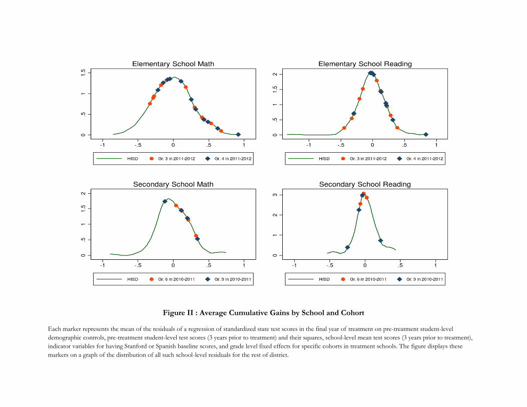
Figure II : Average Cumulative Gains by School and Cohort

Each marker represents the mean of the residuals of a regression of standardized state test scores in the final year of treatment on pre-treatment student-level

demographic controls, pre-treatment student-level test scores (3 years prior to treatment) and their squares, school-level mean test scores (3 years prior to treatment),

indicator variables for having Stanford or Spanish baseline scores, and grade level fixed effects for specific cohorts in treatment schools. The figure displays these

markers on a graph of the distribution of all such school-level residuals for the rest of district.

Table I: Summary of Treatment, Overview

Notes: This table provides an overview of the general components of the field experiments in Houston and Denver and the program in Chicago. The

Denver field experiment was modeled on the Houston field experiment, and thus has almost identical treatment components. In Chicago, the program

was similar, although there were some key differences. For example, in Houston and Denver, tutors worked with all 6th and 9th graders in a 2-to-1 ratio

regardless of their level. In Chicago, tutors worked primarily with struggling students with similar re-teaching needs in groups of five. Additionally, the

Chicago program did not have any apparent evidence of increased time on task. The school day and year were not extended, there was no weekend or

summer programming and after-school programming was typically tied to curricular enhancements such as arts and sports.

Houston Elementary Houston Secondary Denver Chicago

1. Human Capital

Principals Replaced Teachers Removed

2. More Time on Task Extended Day - - Extended Year - - More Efficient Daily Schedule -

3. High-Dosage Tutoring 2-on-1 Tutoring - - 3-on-1 Tutoring

- - 5-on-1 Tutoring - - -

4. Culture of High Expectations Student Goals Posted Visual Evidence of College-going

Culture

5. Data-Driven Instruction

Table IIA: Pre-Treatment Summary Statistics, HoustonElementary Schools

Experimental Sample Full Samplep-val p-val

Treatment Control (1) = (2) Treatment Comparison (4) = (5)(1) (2) (3) (4) (5) (6)

Female 0.488 0.473 0.794 0.480 0.500 0.075White 0.018 0.005 0.207 0.015 0.079 0.001Black 0.257 0.335 0.539 0.324 0.204 0.095Hispanic 0.677 0.621 0.654 0.619 0.648 0.688Asian 0.006 0.008 0.535 0.005 0.033 0.000Economically Disadvantaged 0.939 0.953 0.489 0.945 0.831 0.000Limited English Proficiency 0.505 0.440 0.398 0.470 0.448 0.655Special Education 0.020 0.022 0.451 0.018 0.024 0.119Gifted and Talented 0.144 0.109 0.030 0.140 0.219 0.000Baseline Math Score (TAKS) 600.606 599.298 0.759 594.397 623.464 0.000Baseline Reading Score (TAKS) 606.178 606.735 0.984 600.403 628.977 0.000Baseline Std. Math Score (TAKS) -0.161 -0.186 0.516 -0.254 0.090 0.000Baseline Std. Reading Score (TAKS) -0.149 -0.152 0.807 -0.237 0.084 0.000

Schools 8 8 16 11 168 179Observations 1,824 1,683 3,507 2,255 37,209 39,464

Table IIB: Pre-Treatment Summary Statistics, HoustonMiddle & High Schools All Schools

Full Sample Full Samplep-val p-val

Treatment Comparison (7) = (8) Treatment Comparison (10) = (11)(7) (8) (9) (10) (11) (12)

Female 0.507 0.505 0.837 0.499 0.503 0.640White 0.027 0.094 0.000 0.023 0.088 0.000Black 0.409 0.242 0.001 0.384 0.226 0.000Hispanic 0.540 0.624 0.099 0.563 0.634 0.070Asian 0.024 0.038 0.038 0.018 0.036 0.000Economically Disadvantaged 0.865 0.744 0.000 0.881 0.771 0.000Limited English Proficiency 0.206 0.161 0.111 0.260 0.251 0.775Special Education 0.047 0.037 0.204 0.041 0.033 0.222Gifted and Talented 0.115 0.206 0.000 0.120 0.210 0.000Baseline Math Score (TAKS) 1040.690 1221.673 0.272 910.598 969.863 0.630Baseline Reading Score (TAKS) 1062.220 1240.166 0.285 927.603 982.892 0.658Baseline Std. Math Score (TAKS) -0.135 0.127 0.000 -0.169 0.111 0.000Baseline Std. Reading Score (TAKS) -0.126 0.111 0.000 -0.158 0.100 0.000

Schools 9 115 124 20 262 282Observations 5,481 51,186 56,667 7,736 88,395 96,131

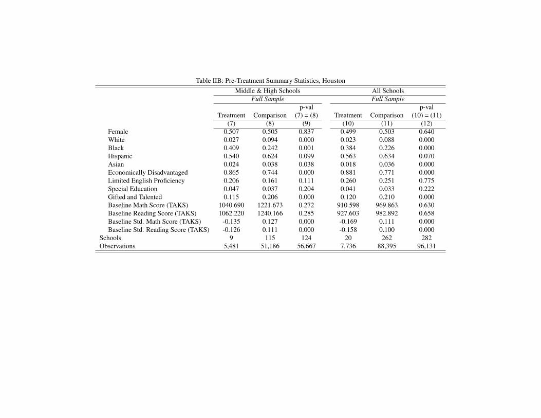
Notes: This table displays pre-treatment student-level summary statistics for various subgroups of our sample. The reported means are from thepre-treatment year in each subsample. Thus, means are reported for 2nd, 3rd, and 4th graders in 2010-2011 since these are the grades that areeligible to receive treatment and have test scores in 2011-2012 (the first year of treatment for elementary schools). For these students, baselinescores are their 2010-2011 Texas Assessment of Knowledge (TAKS) scores (3rd, 4th) or 2010-2011 Stanford scores (2nd). Likewise, 2009-2010means are reported for students scheduled to attend middle and high school in 2010-2011 (the first year of treatment for middle and high schools).For these students, baseline scores are their 2009-2010 TAKS scores. All samples are restricted to those students with valid math and readingbaseline scores and valid math and reading outcome scores in the first year of treatment. The summary statistics for other race students are notshown because no students in our treatment, control, or comparison samples were other race. Columns (1) and (2) report means for students enrolledin Treatment and Control elementary schools in the 2nd - 4th grades during the pre-treatment year (2010-2011). Column (3) reports p-values from atest of equal means, obtained by regressing each variable on a treatment indicator and a matched-pair fixed effect and clustering standard errors byschool. Column (4) reports means for students enrolled in a treatment elementary schools in the 2nd - 4th grades during the 2010-2011 school year.Column (5) reports means for students in these grades enrolled in a comparison elementary school. Column (6) reports p-values from a test of equalmeans with standard errors clustered by school. Column (7) reports means for students in the treatment middle and high school sample. Column(8) reports means for students in these grades who were not in the treatment sample. Column (9) reports p-values from a test of equal means withstandard errors clustered by school. Column (10) reports means for students in Columns (4) and (7). Column (11) reports means for students inColumns (5) and (8). Column (12) reports p-values from a test of equal means with standard errors clustered by school. See Online Appendix B formore detailed variable definitions.

Table III: The Effect of Treatment on State Test Scores, Experimental Elementary School Results in HoustonITT 2SLS (Ever) 2SLS (Years)

2012 2013 Pooled 2012 2013 Pooled 2012 2013 Pooled(1) (2) (3) (4) (5) (6) (7) (8) (9)

Math 0.137∗∗ 0.132∗∗∗ 0.135∗∗∗ 0.155∗∗ 0.149∗∗∗ 0.153∗∗∗ 0.163∗∗ 0.081∗∗∗ 0.112∗∗∗

(0.064) (0.050) (0.051) (0.072) (0.056) (0.057) (0.076) (0.031) (0.042)

3,507 3,121 6,628 3,507 3,121 6,628 3,507 3,121 6,628

Reading 0.018 0.067∗∗ 0.041 0.021 0.076∗∗ 0.046 0.022 0.041∗∗ 0.034(0.044) (0.032) (0.031) (0.050) (0.036) (0.035) (0.052) (0.020) (0.026)

3,507 3,121 6,628 3,507 3,121 6,628 3,507 3,121 6,628

Average Yearsof Treatment 0.844 1.630 1.215 0.955 1.841 1.373

Notes: This table presents the estimates of the effects of being assigned to or attending a treatment school on state test scores: State of TexasAssessment of Academic Readiness (STAAR) in 2012 & 2013. The sample includes all students enrolled in one of the sixteen schools that wereeligible to be randomized into treatment during the pre-treatment year (2010-2011). The sample is restricted each year to those students whohave valid math and reading scores, have valid math and reading baseline scores, and are enrolled in a HISD elementary school. See Table 3 for anaccounting of the number of students in the sample from each cohort. Columns (1), (2), and (3) report Intent-to-Treat (ITT) estimates with treatmentassigned based on pre-treatment enrollment. Columns (4), (5), and (6) report 2SLS estimates and use treatment assignment as an instrument forhaving ever attended a treatment school. Columns (7), (8), and (9) report 2SLS estimates and use treatment assignment to instrument for thenumber of years spent in a treatment school. The dependent variable in all specifications is state test score, standardized to have a mean of zero andstandard deviation one by grade and year. All specifications adjust for the student-level demographic variables summarized in Table 2, student-levelmath and reading scores (3 years prior to 2011-2012) and their squares, and indicator variables for taking a Stanford or Spanish baseline test. Allspecifications have grade year, and matched-pair fixed effects. Average years of treatment provides the expected number of years treated in eachsample conditional on all covariates. This number can be used to scale the 2SLS (Years) estimates into the other estimates i.e. multiplying 0.844and the 2012 2SLS (Years) estimate produces the 2012 ITT estimate. Standard errors (reported in parentheses) are clustered at the current schoollevel. Clustering at the level of the school at time of treatment assignment only changes standard errors trivially. *, *, and *** denote significanceat the 90%, 95%, and 99% confidence levels, respectively.

Table IV: The Effect of Treatment on State Test Scores, Quasi-Experimental Results in HoustonOLS 2SLS (Ever) 2SLS (Years)

2011 2012 2013 Pooled 2011 2012 2013 Pooled 2011 2012 2013 Pooled(1) (2) (3) (4) (5) (6) (7) (8) (9) (10) (11) (12)

Panel A: All Elementary SchoolsMath 0.191∗∗∗ 0.212∗∗∗ 0.202∗∗∗ 0.233∗∗∗ 0.259∗∗∗ 0.246∗∗∗ 0.251∗∗∗ 0.144∗∗∗ 0.184∗∗∗

— (0.068) (0.079) (0.067) — (0.085) (0.095) (0.082) — (0.091) (0.053) (0.060)

39,464 36,010 75,474 39,464 36,010 75,474 39,464 36,010 75,474

Reading 0.071 0.087∗ 0.079∗ 0.086 0.106∗ 0.096∗ 0.093 0.059∗ 0.072∗

— (0.045) (0.051) (0.043) — (0.055) (0.061) (0.052) — (0.059) (0.034) (0.039)

39,464 36,010 75,474 39,464 36,010 75,474 39,464 36,010 75,474

Average Yearsof Treatment 0.763 1.467 1.093 0.931 1.791 1.335

Panel B: All Middle & High SchoolsMath 0.113∗∗∗ 0.090∗∗∗ 0.069∗ 0.102∗∗∗ 0.188∗∗∗ 0.172∗∗∗ 0.190∗∗ 0.191∗∗∗ 0.209∗∗∗ 0.100∗∗∗ 0.077∗∗ 0.146∗∗∗

(0.033) (0.033) (0.039) (0.029) (0.045) (0.056) (0.080) (0.043) (0.049) (0.032) (0.030) (0.031)

56,667 26,457 12,271 95,395 56,667 26,457 12,271 95,395 56,667 26,457 12,271 95,395

Reading -0.014 -0.003 -0.000 -0.008 -0.023 -0.005 -0.000 -0.016 -0.026 -0.003 -0.000 -0.012(0.016) (0.025) (0.024) (0.016) (0.027) (0.048) (0.065) (0.029) (0.030) (0.028) (0.026) (0.022)

56,667 26,457 12,271 95,395 56,667 26,457 12,271 95,395 56,667 26,457 12,271 95,395

Average Yearsof Treatment 0.540 0.896 0.898 0.701 0.899 1.716 2.461 1.308

Notes: This table presents the estimates of the effects of being assigned to or attending a treatment school on state test scores: Texas Assessmentof Knowledge (TAKS) in 2011 and State of Texas Assessment of Academic Readiness in 2012 & 2013. The elementary school sample in Panel Aincludes students enrolled in any of the 8 experimentally selected treatment schools or the 3 non-experimentally selected treatment schools in thepre-treatment year (2011-2012). Panel A also includes a comparison sample of students enrolled in a HISD elementary school in the pre-treatmentyear. The middle and high school sample in Panel B includes all 6th , 7th , 9th , or 10th grade students enrolled in a HISD school in the pre-treatment year (2009-2010), as well as all 6th and 9th graders in 2010-2011 zoned to a HISD school. Those 6th, 7th,9th, and 10th graders enrolledin a treatment school in 2009-2010 and those 6th and 9th graders zoned to attend a treatment school in 2010-2011 are assigned to treatment. Thesamples are restricted in each year to those students who have valid math and reading scores, have valid baseline math and reading scores, and areenrolled in a school that serves the same grade levels as the one they were in when treatment was assigned. Columns (1), (2), (3), and (4) report OLSestimates with treatment based on pre-treatment enrollment for non-entry grades and enrollment zone for entry grades. Columns (5), (6), (7), and(8) report 2SLS estimates and use treatment assignment to instrument for having ever attended a treatment school. Columns (9), (10), (11), and (12)report 2SLS estimates and use treatment assignment to instrument for the number of years spent in a treatment school. The dependent variable inall specifications is the state test score, standardized to have a mean of zero and standard deviation one by grade and year. All specifications adjustfor the student-level demographic variables summarized in Table 2, these demographic variables at the school level, student-level math and readingscores (3 years prior to treatment) and their squares, school-level mean math and reading scores (3 years prior to treatment), and indicator variablesfor taking a Stanford or Spanish baseline test. All specifications have grade and year level fixed effects. Average years of treatment provides theexpected number of years treated in each sample conditional on all covariates. This number can be used to scale the 2SLS (Years) estimates intothe other estimates i.e. multiplying 0.763 and the 2012 2SLS (Years) estimate produces the 2012 ITT school estimate. Standard errors (reported inparentheses) are clustered at the school level. *, *, and *** denote significance at the 90%, 95%, and 99% confidence levels, respectively.

Table V: The Effect of Treatment with High-Dosage Tutoring, HoustonExperimental Results Quasi-Experimental Results

ITT 2SLS (Ever) 2SLS (Years) OLS 2SLS (Ever) 2SLS (Years)(1) (2) (3) (4) (5) (6)

Panel A: Experimental Elementary SchoolsTutoring (4th Grade) 0.181∗∗ 0.205∗∗∗ 0.222∗∗∗ 0.253∗∗∗ 0.294∗∗∗ 0.318∗∗∗

(0.070) (0.078) (0.084) (0.085) (0.098) (0.105)

No Tutoring (5th Grade) 0.140∗∗ 0.158∗∗ 0.172∗∗ 0.163∗∗ 0.187∗∗ 0.202∗∗

(0.060) (0.067) (0.073) (0.078) (0.089) (0.097)

Difference 0.041 0.047 0.050 0.090 0.107 0.116

P-Values 0.407 0.368 0.378 0.094 0.074 0.072

Panel B: All Houston SchoolsElementary Schools

Tutoring (4th Grade) 0.239∗∗∗ 0.294∗∗∗ 0.331∗∗∗

— — — (0.076) (0.093) (0.104)

No Tutoring (5th Grade) 0.180∗∗ 0.216∗∗ 0.242∗∗

— — — (0.071) (0.087) (0.098)

Difference 0.059 0.078 0.089

P-values 0.275 0.231 0.215

Middle & High SchoolsTutoring (6th & 9th Grade) 0.212∗∗∗ 0.535∗∗∗ 0.608∗∗∗

— — — (0.039) (0.075) (0.093)

No Tutoring (7th & 10th Grade) 0.119∗∗∗ 0.182∗∗∗ 0.208∗∗∗

— — — (0.044) (0.056) (0.063)

Difference 0.093 0.353 0.400

P-values 0.007 0.000 0.000

Notes: This table presents estimates of the effects of being assigned to or attending a treatment school and receiving high-dosage tutoring on statetest scores: TAKS in 2011 and STAAR in 2012 & 2013. The difference shown is the treatment effect for the tutoring group minus the treatment effectfor the non-tutoring group. P-values result from a test of equal coefficients between the tutoring and non-tutoring groups. The tutoring elementaryschool group includes students enrolled in the 4th grade during the 2011-2012 and 2012-2013 school years. The tutoring middle and high schoolgroup includes students enrolled in the 6th and 9th grades during the 2010-2011 and 2012-2013 school years. The non-tutoring elementary schoolgroup includes students enrolled in the 5th grade during the 2011-2012 and 2012-2013 school years. The non-tutoring middle and high schoolgroup includes students enrolled in the 7th and 10th grades during the 2010-2011 and 2012-2013 school years. The sample is restricted in eachyear to students with valid math scores, valid math baseline scores, and a valid enrollment zone (entry grades) or pre-treatment HISD enrollment(non-entry grades). Column (1) reports Intent-to-Treat (ITT) estimates with treatment assigned based on pre-treatment enrollment. Column (4)reports OLS estimates with treatment based on pre-treatment enrollment for non-entry grades and enrollment zone for entry grades. Columns(2) and (5) report 2SLS estimates and use treatment assignment to instrument for having ever attended a treatment school. Columns (3) and (6)report 2SLS estimates and use treatment assignment to instrument for the number of years spent in a treatment school. The dependent variable inall specifications is the standardized state math score. All specifications adjust for the student-level demographic variables summarized in Table2, student-level math and reading scores ( 3 years prior to treatment) and their squares, and indicator variables for taking a Stanford or Spanishbaseline test. All specifications have grade and year fixed effects. Columns (1) – (3) also include matched-pair fixed effects. Columns (4) – (6) alsoinclude school-level demographic variables and mean test scores (3 years prior to treatment). Standard errors (reported in parentheses) are clusteredat the school level. *, *, and *** denote significance at the 90%, 95%, and 99% confidence levels, respectively.

Table VI: The Effect of Treatment on State Test Scores, Subgroups in HoustonWhole Gender Race Baseline Test TercileSample Male Female p-val Black Hispanic p-val T1 T2 T3 p-val

(1) (2) (3) (4) (5) (6) (7) (8) (9) (10) (11)Panel A: All Elementary Schools

Math 0.184∗∗∗ 0.159∗∗ 0.213∗∗∗ 0.103 0.225∗∗∗ 0.169∗∗∗ 0.228∗∗∗ 0.197∗∗∗

(0.060) (0.065) (0.056) 0.009 (0.065) (0.068) 0.071 (0.061) (0.081) (0.075) 0.35775,474 37,762 37,705 15,371 49,348 20,834 22,140 20,362

Reading 0.072∗ 0.050 0.099∗∗ 0.039 0.090∗∗ 0.087∗ 0.082 0.036(0.039) (0.039) (0.041) 0.007 (0.063) (0.042) 0.406 (0.048) (0.053) (0.056) 0.38475,474 37,762 37,705 15,371 49,348 20,226 22,384 20,725

Panel B: Middle & High SchoolsMath 0.146∗∗∗ 0.169∗∗∗ 0.124∗∗∗ 0.065 0.198∗∗∗ 0.116∗∗∗ 0.178∗∗∗ 0.193∗∗∗

(0.031) (0.034) (0.033) 0.077 (0.043) (0.029) 0.000 (0.030) (0.033) (0.051) 0.01295,395 47,165 48,174 24,674 59,613 31,567 34,208 29,620

Reading -0.012 -0.011 -0.017 -0.047 0.011 -0.018 0.007 -0.053(0.022) (0.026) (0.025) 0.817 (0.030) (0.022) 0.049 (0.020) (0.024) (0.046) 0.36695,395 47,165 48,174 24,674 59,613 33,301 38,255 23,839

Notes: This table presents estimates of the effects of attending a treatment school on state test scores: TAKS in 2011 and STAAR in 2012 & 2013. All estimates use the quasi-experimental 2SLS (Years)estimator described in the notes of Table 5 and in the text. Elementary school samples are identical to Panel A of Table 5 and middle & high school samples are identical to Panel B of Table 5. Columns (4),(7) and (11) report p-values resulting from a test of equal coefficients between the gender, race, and previous year test score subgroups, respectively. Standard errors (reported in parentheses) are clusteredat the school level. *, *, and *** denote significance at the 90%, 95%, and 99% confidence levels, respectively.

Table VII: The Effect of Treatment On Stanford 10 Scores, HoustonExperimental Results Quasi-Experimental Results

ITT 2SLS (Ever) 2SLS (Years) OLS 2SLS (Ever) 2SLS (Years)(1) (2) (3) (4) (5) (6)

Panel A: Experimental Elementary SchoolsMath 0.102∗∗∗ 0.116∗∗∗ 0.085∗∗∗ 0.133∗ 0.150∗∗ 0.109∗∗

(0.039) (0.044) (0.032) (0.068) (0.076) (0.055)7,029 7,029 7,029 77,955 77,955 77,955

Reading 0.057∗ 0.065∗ 0.047∗ 0.054 0.061 0.045(0.031) (0.035) (0.026) (0.042) (0.048) (0.034)7,029 7,029 7,029 77,955 77,955 77,955

Panel B: All Houston SchoolsElementary Schools

Math 0.129∗∗ 0.152∗∗ 0.114∗∗

— — — (0.060) (0.070) (0.052)78,850 78,850 78,850

Reading 0.044 0.052 0.039— — — (0.040) (0.047) (0.035)

78,850 78,850 78,850

Middle & High SchoolsMath 0.045∗∗ 0.076∗∗ 0.062∗∗

— — — (0.022) (0.038) (0.031)88,542 88,542 88,542

Reading 0.002 0.003 0.002— — — (0.015) (0.025) (0.021)

88,542 88,542 88,542

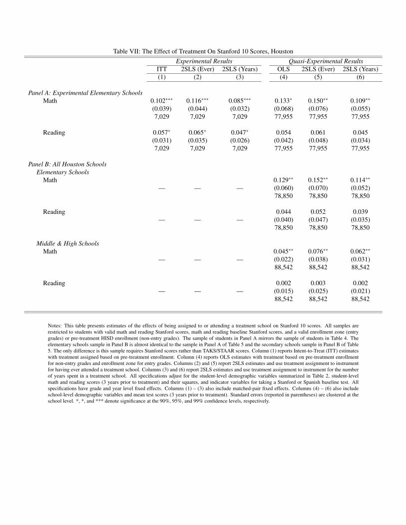
Notes: This table presents estimates of the effects of being assigned to or attending a treatment school on Stanford 10 scores. All samples arerestricted to students with valid math and reading Stanford scores, math and reading baseline Stanford scores, and a valid enrollment zone (entrygrades) or pre-treatment HISD enrollment (non-entry grades). The sample of students in Panel A mirrors the sample of students in Table 4. Theelementary schools sample in Panel B is almost identical to the sample in Panel A of Table 5 and the secondary schools sample in Panel B of Table5. The only difference is this sample requires Stanford scores rather than TAKS/STAAR scores. Column (1) reports Intent-to-Treat (ITT) estimateswith treatment assigned based on pre-treatment enrollment. Column (4) reports OLS estimates with treatment based on pre-treatment enrollmentfor non-entry grades and enrollment zone for entry grades. Columns (2) and (5) report 2SLS estimates and use treatment assignment to instrumentfor having ever attended a treatment school. Columns (3) and (6) report 2SLS estimates and use treatment assignment to instrument for the numberof years spent in a treatment school. All specifications adjust for the student-level demographic variables summarized in Table 2, student-levelmath and reading scores (3 years prior to treatment) and their squares, and indicator variables for taking a Stanford or Spanish baseline test. Allspecifications have grade and year level fixed effects. Columns (1) – (3) also include matched-pair fixed effects. Columns (4) – (6) also includeschool-level demographic variables and mean test scores (3 years prior to treatment). Standard errors (reported in parentheses) are clustered at theschool level. *, *, and *** denote significance at the 90%, 95%, and 99% confidence levels, respectively.

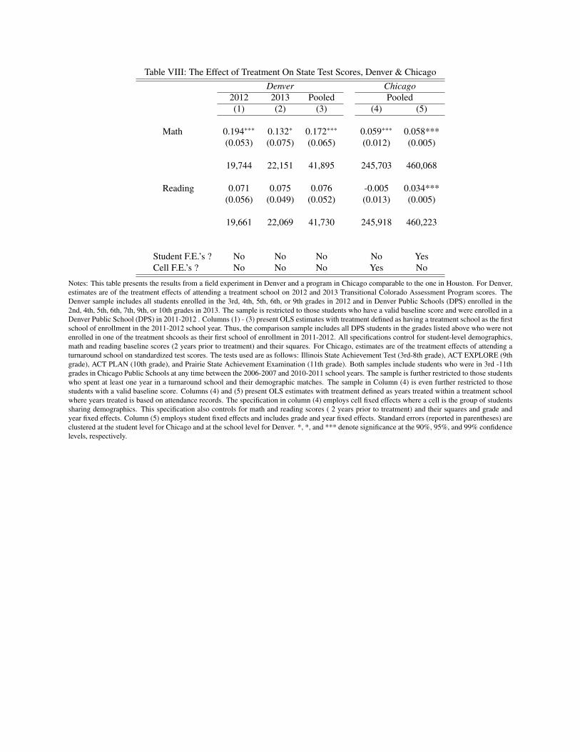
Table VIII: The Effect of Treatment On State Test Scores, Denver & ChicagoDenver Chicago

2012 2013 Pooled Pooled(1) (2) (3) (4) (5)

Math 0.194∗∗∗ 0.132∗ 0.172∗∗∗ 0.059∗∗∗ 0.058***(0.053) (0.075) (0.065) (0.012) (0.005)

19,744 22,151 41,895 245,703 460,068

Reading 0.071 0.075 0.076 -0.005 0.034***(0.056) (0.049) (0.052) (0.013) (0.005)

19,661 22,069 41,730 245,918 460,223

Student F.E.’s ? No No No No YesCell F.E.’s ? No No No Yes No

Notes: This table presents the results from a field experiment in Denver and a program in Chicago comparable to the one in Houston. For Denver,estimates are of the treatment effects of attending a treatment school on 2012 and 2013 Transitional Colorado Assessment Program scores. TheDenver sample includes all students enrolled in the 3rd, 4th, 5th, 6th, or 9th grades in 2012 and in Denver Public Schools (DPS) enrolled in the2nd, 4th, 5th, 6th, 7th, 9th, or 10th grades in 2013. The sample is restricted to those students who have a valid baseline score and were enrolled in aDenver Public School (DPS) in 2011-2012 . Columns (1) - (3) present OLS estimates with treatment defined as having a treatment school as the firstschool of enrollment in the 2011-2012 school year. Thus, the comparison sample includes all DPS students in the grades listed above who were notenrolled in one of the treatment shcools as their first school of enrollment in 2011-2012. All specifications control for student-level demographics,math and reading baseline scores (2 years prior to treatment) and their squares. For Chicago, estimates are of the treatment effects of attending aturnaround school on standardized test scores. The tests used are as follows: Illinois State Achievement Test (3rd-8th grade), ACT EXPLORE (9thgrade), ACT PLAN (10th grade), and Prairie State Achievement Examination (11th grade). Both samples include students who were in 3rd -11thgrades in Chicago Public Schools at any time between the 2006-2007 and 2010-2011 school years. The sample is further restricted to those studentswho spent at least one year in a turnaround school and their demographic matches. The sample in Column (4) is even further restricted to thosestudents with a valid baseline score. Columns (4) and (5) present OLS estimates with treatment defined as years treated within a treatment schoolwhere years treated is based on attendance records. The specification in column (4) employs cell fixed effects where a cell is the group of studentssharing demographics. This specification also controls for math and reading scores ( 2 years prior to treatment) and their squares and grade andyear fixed effects. Column (5) employs student fixed effects and includes grade and year fixed effects. Standard errors (reported in parentheses) areclustered at the student level for Chicago and at the school level for Denver. *, *, and *** denote significance at the 90%, 95%, and 99% confidencelevels, respectively.