INSTITUTE OF AERONAUTICAL ENGINEERING · 4 | P a g e ATTAINMENT OF PROGRAM OUTCOMES& PROGRAM...

1 | P a g e

POWER SYSTEM COMPUTATIONALLABORATORY

LAB MANUAL

Subject Code : BPSB09

Regulations : R18 – IARE

Class : M.Tech I Semester (EPS)

DEPARTMENT OF ELECTRICAL AND ELECTRONICS ENGINEERING

INSTITUTE OF AERONAUTICAL ENGINEERING (Autonomous)

Dundigal – 500 043, Hyderabad

2 | P a g e

INSTITUTE OF AERONAUTICAL ENGINEERING (Autonomous)

Dundigal, Hyderabad - 500 043

Department of Electrical and Electronics Engineering

PROGRAMME EDUCATIONAL OBJECTIVES (PEOs)

The students of M.TechElectrical Power Systemsare prepared to:

PEOI: Impartengineering knowledge in specific and re-equip with latest technologies to analyze,

synthesize the problems in power system and multidisciplinary sectors.

PEOII: Design, develop innovative products and services in the field of electrical power systems with the

latest technology and toolset.

PEOIII: Inculcate research attitude and life-long learning for a successful career.

PEOIV: Attain intellectual leadership skills to cater the needs of power industry, academia, society and

environment.

PROGRAMME OUTCOMES (POs)

Upon completion of M.TechElectrical Power Systems,the students will be able to:

PO1: Identify, formulate and solve power system related problems usingadvanced level computing

techniques.

PO2: Explore ideas to carry out research / investigation independently to solve practical problems

throughcontinuing education.

PO3: Demonstrate knowledge and execute projects on contemporary issues in multidisciplinary

environment.

PO4: Ability to write and present a substantial technical report / document.

PO5: Inculcate ethics, professionalism, multidisciplinary approach, entrepreneurial thinking and effective

communication skills.

PO6: Function effectively as an individual or a leader in a team to propagate ideas and promote teamwork.

PO 7: Develop confidence for self-study and to engage in lifelong learning.

3 | P a g e

INDEX

S No. List of Experiments Page No.

1 Formation of Bus Admittance Matrix

2 Singular Transformation

3 Gauss -Seidel Load Flow Method

4 Newton - Raphson Load Flow Method

5 Fast Decoupled Load Flow Method

6 DC Load Flow

7 Building Algorithm

8 Short Circuit Analysis

9 Transient Stability

10 Load Dispatch Problem

11 Dynamic Programming Method

12 State Estimation

4 | P a g e

ATTAINMENT OF PROGRAM OUTCOMES& PROGRAM SPECIFIC OUTCOMES

Exp. No Experiment Program Outcomes Attained

1 Formation of Bus Admittance Matrix PO1, PO2, PO3

2 Singular Transformation PO1, PO2, PO3

3 Gauss -Seidel Load Flow Method PO1, PO2, PO3

4 Newton - Raphson Load Flow Method PO1, PO2, PO3

5 Fast Decoupled Load Flow Method PO1, PO2, PO3

6 DC Load Flow PO1, PO2, PO3

7 Building Algorithm PO1, PO2, PO3, PO4

8 Short Circuit Analysis PO2, PO3

9 Transient Stability PO1, PO2, PO3, PO4

10 Load Dispatch Problem PO2, PO3

11 Dynamic Programming Method PO2, PO3

12 State Estimation PO2, PO3, PO4

5 | P a g e

POWER SYSTEM COMPUTATIONALLABORATORY

OBJECTIVE

The objective of power system computational laboratory is to analyze electrical power system in steady state

and transient state. In steady state the power system parameters are obtained by different load flow methods.

In transient state the system stability is analyzed. Also, the formation of Ybus and Zbus is explained. In

addition to this, the other methods of power system analysis mentioned here are unit commitment and state

estimation. The simulation tool adopted is MATLAB.

OUTCOMES:

Upon the completion of Power Systems Computational Laboratory practical course, the student will be able

to attain the following:

1. Develop a MATLAB program for [Y]bus formation by direct inspection method and singular

transformation method.

2. Estimate the steady state parameters in power system is by Gauss -Seidal load flow method, Newton -

Raphson load flow method, Fast Decoupledload flow method and DC Load Flow.

3. Construct ZBUS matrix which is a prerequisite to analyze the power system in case of fault.

4. Determine a MATLAB program for short circuit analysis.

5. Determine the economic operation of power systems through economic load dispatch.

6. Recognize the optimal number of generators to supply the load demand by means of unit commitment.

7. Estimate the state of electrical power system.

6 | P a g e

EXPERIMENT - 1

FORMATION OF BUS ADMITTANCE MATRIX

1.1 AIM:

To develop a program for Ybus formation by direct inspection method.

1.2 APPARATUS:

Desktop Computers with MATLAB software

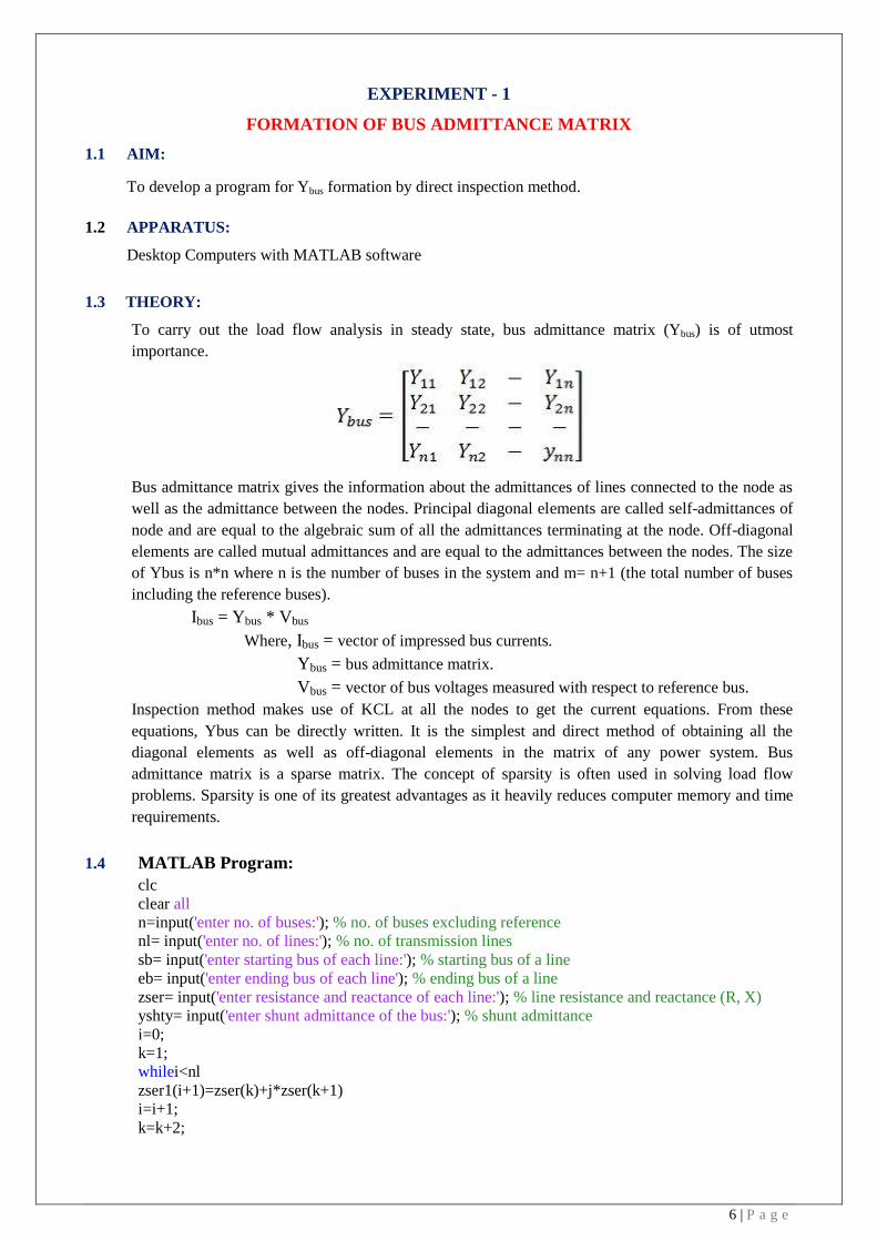
1.3 THEORY:

To carry out the load flow analysis in steady state, bus admittance matrix (Ybus) is of utmost

importance.

Bus admittance matrix gives the information about the admittances of lines connected to the node as

well as the admittance between the nodes. Principal diagonal elements are called self-admittances of

node and are equal to the algebraic sum of all the admittances terminating at the node. Off-diagonal

elements are called mutual admittances and are equal to the admittances between the nodes. The size

of Ybus is n*n where n is the number of buses in the system and m= n+1 (the total number of buses

including the reference buses).

Ibus = Ybus * Vbus

Where, Ibus = vector of impressed bus currents.

Ybus = bus admittance matrix.

Vbus = vector of bus voltages measured with respect to reference bus.

Inspection method makes use of KCL at all the nodes to get the current equations. From these

equations, Ybus can be directly written. It is the simplest and direct method of obtaining all the

diagonal elements as well as off-diagonal elements in the matrix of any power system. Bus

admittance matrix is a sparse matrix. The concept of sparsity is often used in solving load flow

problems. Sparsity is one of its greatest advantages as it heavily reduces computer memory and time

requirements.

1.4 MATLAB Program:

clc

clear all

n=input('enter no. of buses:'); % no. of buses excluding reference

nl= input('enter no. of lines:'); % no. of transmission lines

sb= input('enter starting bus of each line:'); % starting bus of a line

eb= input('enter ending bus of each line'); % ending bus of a line

zser= input('enter resistance and reactance of each line:'); % line resistance and reactance (R, X)

yshty= input('enter shunt admittance of the bus:'); % shunt admittance

i=0;

k=1;

whilei<nl

zser1(i+1)=zser(k)+j*zser(k+1)

i=i+1;

k=k+2;

7 | P a g e

end

zser2=reshape(zser1,nl,1);

yser=ones(nl,1)./zser2;

ybus=zeros(n,n);

fori=1:nl

ybus(sb(i),sb(i))=ybus(sb(i),sb(i))+(j*yshty(i))+yser(i);

ybus(eb(i),eb(i))=ybus(eb(i),eb(i))+(j*yshty(i))+yser(i);

ybus(sb(i),eb(i))=-yser(i);

ybus(eb(i),sb(i))=-yser(i);

end

ybus

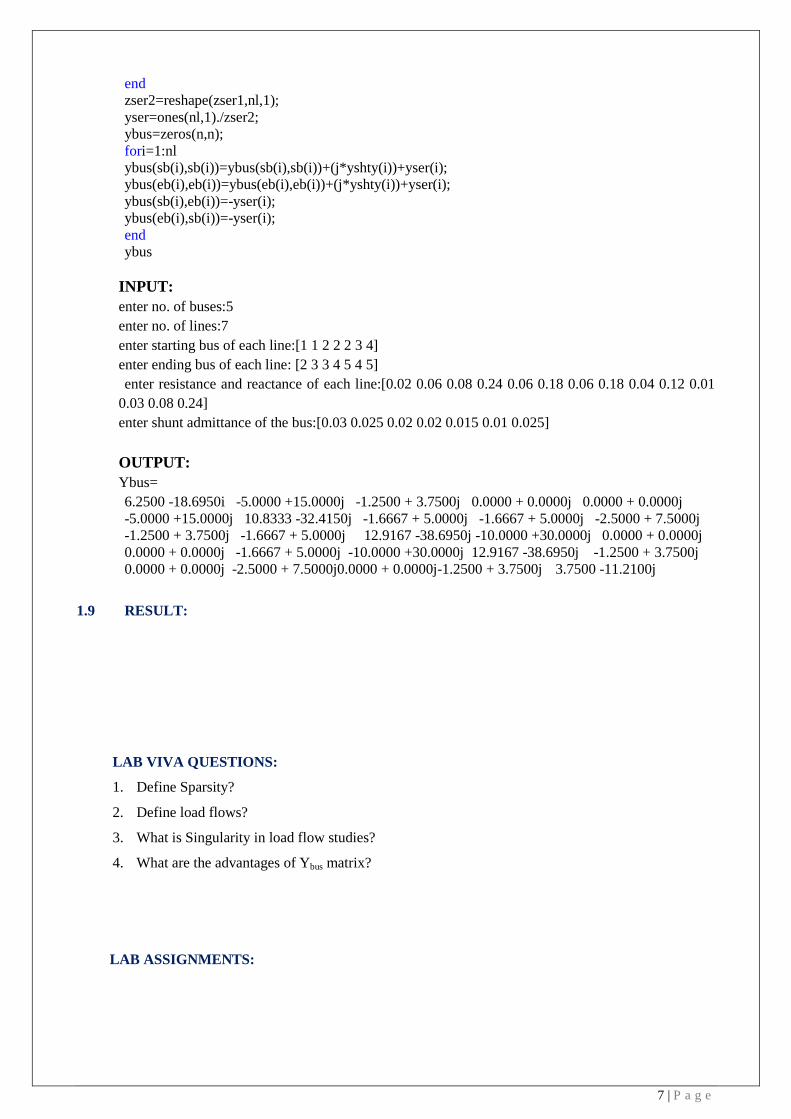
INPUT:

enter no. of buses:5

enter no. of lines:7

enter starting bus of each line:[1 1 2 2 2 3 4]

enter ending bus of each line: [2 3 3 4 5 4 5]

enter resistance and reactance of each line:[0.02 0.06 0.08 0.24 0.06 0.18 0.06 0.18 0.04 0.12 0.01

0.03 0.08 0.24]

enter shunt admittance of the bus:[0.03 0.025 0.02 0.02 0.015 0.01 0.025]

OUTPUT:

Ybus=

6.2500 -18.6950i -5.0000 +15.0000j -1.2500 + 3.7500j 0.0000 + 0.0000j 0.0000 + 0.0000j

-5.0000 +15.0000j 10.8333 -32.4150j -1.6667 + 5.0000j -1.6667 + 5.0000j -2.5000 + 7.5000j

-1.2500 + 3.7500j -1.6667 + 5.0000j 12.9167 -38.6950j -10.0000 +30.0000j 0.0000 + 0.0000j

0.0000 + 0.0000j -1.6667 + 5.0000j -10.0000 +30.0000j 12.9167 -38.6950j -1.2500 + 3.7500j

0.0000 + 0.0000j -2.5000 + 7.5000j0.0000 + 0.0000j-1.2500 + 3.7500j 3.7500 -11.2100j

1.9 RESULT:

LAB VIVA QUESTIONS:

1. Define Sparsity?

2. Define load flows?

3. What is Singularity in load flow studies?

4. What are the advantages of Ybus matrix?

LAB ASSIGNMENTS:

8 | P a g e

EXPERIMENT –2

SINGULAR TRANSFORMATION

2.1 AIM:

To develop a program forYbusformation by singular transformation method

2.2 APPARATUS:


2.3 THEORY:

The admittancematrix is designated asYbus. This matrix is asymmetric and square matrix that

completely describes the configuration of power transmission lines. In realistic systems, which are

quite large containing thousands of buses, the admittance matrix is quite sparse. Each bus in a real

time power system is usually connected to only a few other buses through the transmission lines.

Ybus can be alternatively constitutedwith singular transformation, given by a network topology. This

alternative approach is of great theoretical and practical significance.

The algorithm for obtaining Ybus using singular transformation method is given as follows:

Step 1: Obtain the oriented graph for the given system.

Step 2: Get the bus incidence matrix which is the one which indicates the incidence of all the

elements to nodes in connected graph. The size of this matrix is e*(n-1) where „e‟ is the number of

elements in the graph and „n‟ is the number of nodes

Step 3: Get the primitive admittance matrix from the graph of size [e*e]. If mutual coupling

between the lines is neglected then the resulting primitive matrix is a diagonal matrix(off-diagonal

elements are zero)

Step 4: Ybus can be obtained from the equation, Ybus = AT * [y] *A

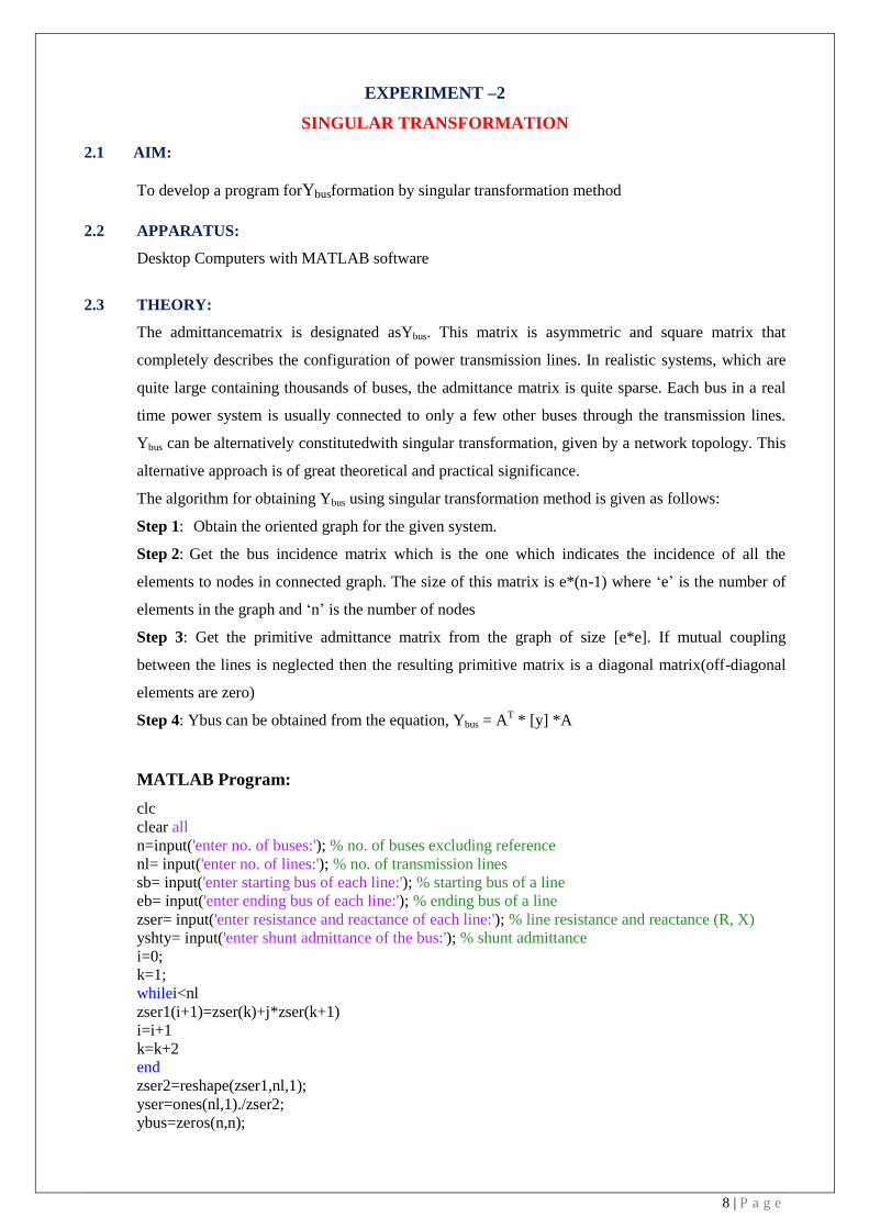
MATLAB Program:

clc

clear all

n=input('enter no. of buses:'); % no. of buses excluding reference

nl= input('enter no. of lines:'); % no. of transmission lines

sb= input('enter starting bus of each line:'); % starting bus of a line

eb= input('enter ending bus of each line:'); % ending bus of a line

zser= input('enter resistance and reactance of each line:'); % line resistance and reactance (R, X)

yshty= input('enter shunt admittance of the bus:'); % shunt admittance

i=0;

k=1;

whilei<nl

zser1(i+1)=zser(k)+j*zser(k+1)

i=i+1

k=k+2

end

zser2=reshape(zser1,nl,1);

yser=ones(nl,1)./zser2;

ybus=zeros(n,n);

9 | P a g e

ypri=zeros(nl+n, nl+n);

a=zeros(nl+n,n);

fori=1:n

a(i,i)=1;

end

fori=1:nl

a(n+i,sb(i))=1;

a(n+i,eb(i))=-1;

ypri(n+i,n+i)=yser(i);

ypri(sb(i),sb(i))=ypri(sb(i),sb(i))+yshty(i);

ypri(eb(i),eb(i))=ypri(sb(i),eb(i))+yshty(i);

end

at=transpose(a);

ybus=at*ypri*a

zbus=inv(ybus)

INPUT:

enter no. of buses:3

enter no. of lines:3

enter starting bus of each line:[1 1 2]

enter ending bus of each line:[2 3 3]

enter resistance and reactance of each line:[0.01 0.03 0.08 0.24 0.06 0.18]

enter shunt admittance of the bus:[0.01 0.025 0.02]

OUTPUT:

Ybus:

11.2850 -33.7500j -10.0000 +30.0000j -1.2500 + 3.7500j

-10.0000 +30.0000j 11.6967 -35.0000j -1.6667 + 5.0000j

-1.2500 + 3.7500j -1.6667 + 5.0000j 2.9367 - 8.7500j

RESULT:

LAB VIVA QUESTIONS:

1. For n bus power system, what is the size of Ybus matrix?

2. Which matrix is used for load flow studies?

3. What is the sparsity of Y bus matrix of a 4 bus power system consists of 4 transmission lines?

LAB ASSIGNMENTS:

10 | P a g e

EXPERIMENT –3

GAUSS – SEIDAL LOAD FLOW METHOD

3.1 AIM:

To develop a program for Gauss - Seidal load flow algorithm.

3.2 APPARATUS:


3.3 THEORY:

Load flow analysis is the study conducted to determine the steady state operating condition of the

given system under given conditions. A large number of numerical algorithms have been developed

and Gauss Seidel method is one of such algorithm.

2.4 Problem Formulation:

The performance equation of the power system may be written as

[Ibus] = [Ybus][Vbus] (1)

Selecting one of the buses as the reference bus, we get (n-1) simultaneous equations.

The bus loading equations can be written as

Ii = Pi-jQi / Vi* (i=1,2,3,…………..n) (2)

where, Pi=Re [ 𝑉𝑖𝑛𝑘=1 ∗ 𝑌𝑖𝑘𝑉𝑘] . (3)

Qi= -Im [ 𝑉𝑖𝑛𝑘=1 ∗ 𝑌𝑖𝑘𝑉𝑘]. (4)

The bus voltage can be written in form of

Vi=(1.0/Yii)[Ii- 𝑌𝑖𝑗𝑛𝑗=1 𝑗≠𝑖

𝑉𝑗 ] (i=1,2,…………n)&i≠slack bus (5)

Substituting Ii in the expression for Vi, we get

Vinew=(1.0/Yii)[Pi-jQi / Vi0* - 𝑌𝑖𝑗𝑛𝑗=1 𝑉𝑖0] (6)

The latest available voltages are used in the above expression, we get

Vinew=(1.0/Yii)[Pi-jQi / 𝑉𝑖0* - 𝑌𝑖𝑗

𝑛𝑗=1 𝑉𝑗

𝑛 - 𝑌𝑖𝑗𝑛𝑗=𝑖+1 . 𝑉𝑖0] (7)

These equations can be solved for voltages in interactive manner. During each iteration, it

cancompute all the bus voltages and check for convergence, which is carried out by comparison with

the voltages obtained at the end of previous iteration. After the solutions is obtained, the stack bus

real and reactive powers, the reactive power generation at other generator buses and line flows can

be calculated.

ALGORITHM:

Step1: Read the data such as line data, specified power, specified voltages, Q limits at the generator

buses and tolerance for convergences.

Step2: Compute Y-bus matrix.

11 | P a g e

Step3: Initialize all the bus voltages.

Step4:Iteration count, Iter=1

Step5: Consider i=2, where „i‟ is the bus number.

Step6:Check whether this is PV bus or PQ bus. If it is PQ bus goto step 8 otherwise go to next step.

Step7: Compute Qi check for Q limit violation.

QGi=Qi+QLi.

If QGi>Qi max,equate QGi = Qimax. Then convert it into PQ bus.

If QGi˂Qi min,equate QGi = Qimin. Then convert it into PQ bus.

Step 8: Calculate the new value of the bus voltage using Gauss Seidal formula.

Vi=(1.0/Yii) [(Pi-j Qi)/Vi0*- 𝑌𝑖𝑗𝑛𝑗=1 Vj- 𝑌𝑖𝑗

𝑛𝑗=𝑖+1 Vj0]

Adjust voltage magnitude of the bus to specify magnitude if Q limits are not violated.

Step 9: If all buses are considered go to step 10, otherwise increments the bus count, bus no. i=i+1

and go to step6.

Step 10: Check for convergence. If there is no convergence goes to step 11, otherwise go to step12.

Step 11: Update the bus voltage using static load flow equation.

Vinew=Viold+ α(Vinew-Viold);i=1,2,…..n,i≠ slackbus,„α‟ is the acceleration factor=1.4

Step 12: Calculate the slack bus power, reactive power at PV buses, real and reactive powers at load

buses and line losses.Print all the results including all the bus voltages and all the bus angles.

Step 13: Stop.

MATLAB PROGRAM: clc

clear all

n=3;

V=[1.05 1 1];

Y=[20-j*50 -10+j*20 -10+j*30; -10+j*20 26-j*52 -16+j*32; -10+j*30 -16+j*32 26-j*62] ;

P=[inf -2.566 -1.386];

Q=[inf -1.102 -0.452];

iter=10;

Vprev=V;

foriter=1:10

abs(V);

abs(Vprev);

Vprev=V;

sumyv=[0 0 0 0];

fori=2:n

for k=1:n,

if(i~=k)

sumyv(i)=sumyv(i)+(Y(i,k)*V(k));

end

end

V(i)=(1/Y(i,i))*((P(i)-j*Q(i))/conj(V(i))-sumyv(i))

iter

end

end

12 | P a g e

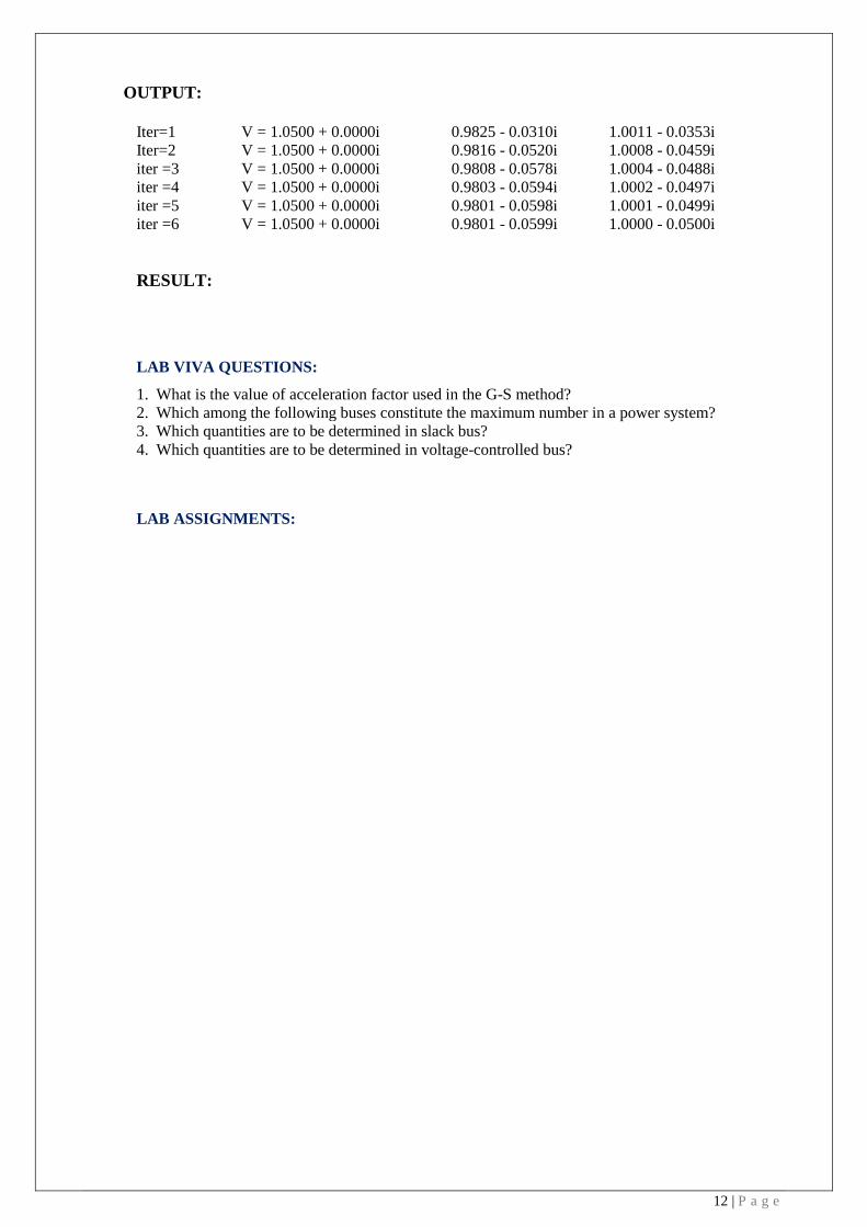
OUTPUT:

Iter=1 V = 1.0500 + 0.0000i 0.9825 - 0.0310i 1.0011 - 0.0353i

Iter=2 V = 1.0500 + 0.0000i 0.9816 - 0.0520i 1.0008 - 0.0459i

iter =3 V = 1.0500 + 0.0000i 0.9808 - 0.0578i 1.0004 - 0.0488i

iter =4 V = 1.0500 + 0.0000i 0.9803 - 0.0594i 1.0002 - 0.0497i

iter =5 V = 1.0500 + 0.0000i 0.9801 - 0.0598i 1.0001 - 0.0499i

iter =6 V = 1.0500 + 0.0000i 0.9801 - 0.0599i 1.0000 - 0.0500i

RESULT:

LAB VIVA QUESTIONS:

1. What is the value of acceleration factor used in the G-S method?

2. Which among the following buses constitute the maximum number in a power system?

3. Which quantities are to be determined in slack bus?

4. Which quantities are to be determined in voltage-controlled bus?

LAB ASSIGNMENTS:

13 | P a g e

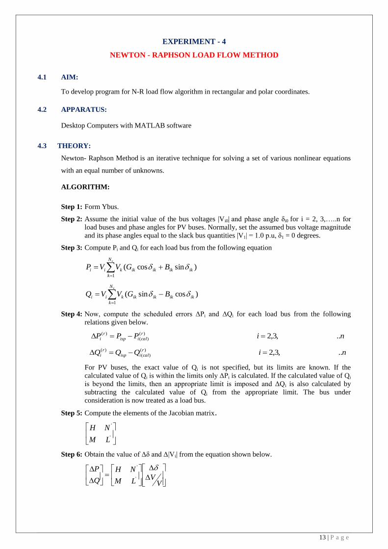
EXPERIMENT - 4

NEWTON - RAPHSON LOAD FLOW METHOD

4.1 AIM:

To develop program for N-R load flow algorithm in rectangular and polar coordinates.

4.2 APPARATUS:


4.3 THEORY:

Newton- Raphson Method is an iterative technique for solving a set of various nonlinear equations

with an equal number of unknowns.

ALGORITHM:

Step 1: Form Ybus.

Step 2: Assume the initial value of the bus voltages |Vi0| and phase angle δi0 for i = 2, 3,…..n for

load buses and phase angles for PV buses. Normally, set the assumed bus voltage magnitude

and its phase angles equal to the slack bus quantities |V1| = 1.0 p.u, δ1 = 0 degrees.

Step 3: Compute Pi and Qi for each load bus from the following equation

vN

k

ikikikikkii BGVVP1

)sincos(

vN

k

ikikikikkii BGVVQ1

)cossin(

Step 4: Now, compute the scheduled errors ΔPi and ΔQi for each load bus from the following

relations given below.

niPPP r

caliisp

r

i ..,3,2)(

)(

)(

niQQQ r

caliisp

r

i ..,3,2)(

)(

)(

For PV buses, the exact value of Qi is not specified, but its limits are known. If the

calculated value of Qi is within the limits only ΔPi is calculated. If the calculated value of Qi

is beyond the limits, then an appropriate limit is imposed and ΔQi is also calculated by

subtracting the calculated value of Qi from the appropriate limit. The bus under

consideration is now treated as a load bus.

Step 5: Compute the elements of the Jacobian matrix.

'

'

LM

NH

Step 6: Obtain the value of Δδ and Δ|Vi| from the equation shown below.

VV

LM

NH

Q

P

'

'

14 | P a g e

Step 7: Using the values of Δδi and Δ|Vi| calculated in the above step, modify the voltage magnitude

and phase angle at all load buses by the equations shown below.

)()()1( r

i

r

i

r

i VVV

)()()1( r

i

r

i

r

i

Step 8: Start the next iteration cycle following the step 2 with the modified values of |Vi|and δi.

Step 9: Continue until scheduled errors for all the load buses are within a specified tolerance that is

,, )()( r

i

r

i QandP

where, ε denotes the tolerance level for load buses.

Step 10:Calculate the line and power flow at the slack bus

MATLAB PROGRAM:

clear all;

v=[1.05 1 1.04];

d=[0;0;0];

Ps=[-4;2];

Qs=-2.5;

yb=[20-j*50 -10+j*20 -10+j*30;-10+j*20 26-j*52 -16+j*32;-10+j*30 -16+j*32 26-j*62];

y=abs(yb);

t=angle(yb);

iter=0;

pwracur=0.00025;

DC=10;

while max(abs(DC))>pwracur

iter=iter+1

p=[v(2)*v(1)*y(2,1)*cos(t(2,1)-d(2)+d(1))+v(2)^2*y(2,2)*cos(t(2,2))+v(2)*v(3)*y(2,3)*cos(t(2,3)-

d(2)+d(3));v(3)*v(1)*y(3,1)*cos(t(3,1)-

d(3)+d(1))+v(3)^2+y(3,3)*cos(t(3,3))+v(3)*v(2)*y(3,2)*cos(t(3,2)-d(3)+d(2))];

q=-v(2)*v(1)*y(2,1)*sin(t(2,1)-d(2)+d(1))-v(2)^2*y(2,2)*sin(t(2,2))-v(2)*v(3)*y(2,3)*sin(t(2,3)-

d(2)+d(3));

j(1,1)=v(2)*v(1)*y(2,1)*sin(t(2,1)-d(2)+d(1))+v(2)*v(3)*y(2,3)*sin(t(2,3)-d(2)+d(3));

j(1,2)=-v(2)*v(3)*y(2,3)*sin(t(2,3)-d(2)+d(3));

j(1,3)=v(1)*y(2,1)*cos(t(2,1)-d(2)+d(1))+2*v(2)*y(2,2)*cos(t(2,2))+v(3)*y(2,3)*cos(t(2,3)-

d(2)+d(3));

j(2,1)=-v(3)*v(2)*y(3,2)*sin(t(3,2)-d(3)+d(2));

j(2,2)=v(3)*v(2)*y(3,1)*sin(t(3,1)-d(3)+d(1))+v(3)*v(2)*y(3,2)*sin(t(3,2)-d(3)+d(2));

j(2,3)=v(3)*y(2,3)*cos(t(3,2)-d(3)+d(2));

j(3,1)=v(2)*v(1)*y(2,1)*cos(t(2,1)-d(2)+d(1))+v(2)*v(3)*y(2,3)*cos(t(2,3)-d(2)+d(3));

j(3,2)=-v(2)*v(3)*y(2,3)*cos(t(2,3)-d(2)+d(3));

j(3,3)=-v(1)*y(2,1)*sin(t(2,1)-d(2)+d(1))-2*v(2)*y(2,2)*sin(t(2,2))-v(3)*y(2,3)*sin(t(2,3)-

d(1)+d(3));

DP=Ps-p;

DQ=Qs-q;

DC=[DP;DQ]

j

DX=j\DC

d(2)=d(2)+DX(1);

d(3)=d(3)+DX(2);

v(2)=v(2)+DX(3);

v,d,delta=180/pi*d;

end

15 | P a g e

p1=v(1)^2*y(1,1)*cos(t(1,1))+v(1)*v(2)*y(1,2)*cos(t(1,2)-d(1)+d(2))+v(1)*v(3)*y(1,3)*cos(t(1,3)-

d(1)+d(3))

q1=-v(1)^2*y(1,1)*sin(t(1,1))-v(1)*v(2)*y(1,2)*sin(t(1,2)-d(1)+d(2))-v(1)*v(3)*y(1,3)*sin(t(1,3)-

d(1)+d(3))

q3=-v(3)*v(1)*y(3,1)*sin(t(3,1)-d(3)+d(1))-v(3)*v(2)*y(3,2)*sin(t(3,2)-d(3)+d(2))-

v(3)^2*y(3,3)*sin(t(3,3))

OUTPUT:

iter = 1

DC = -2.8600 2.4784 -0.2200

j = 54.2800 -33.2800 24.8600 -33.2800 64.4800 -16.6400 -27.1400 16.6400 49.7200

DX = -0.0310 -0.0156 -0.0265

v = 1.0500 0.9735 1.0400

d = 0 -0.0310 -0.0156

iter = 2

DC = -0.0998 0.0015 -0.0520

j = 51.7235 -31.6073 21.3032 -33.1154 63.6413 -15.0727 -28.5380 17.6888 47.5578

DX = -0.0021 -0.0016 -0.0018

v = 1.0500 0.9717 1.0400

d = 0 -0.0331 0.0140

iter = 3

DC = -0.0002 0.0038 0.0008

j = 51.5944 -31.5386 21.1465 - -33.0626 63.5170 -15.0530 -28.5466 17.6743 47.3677

DX = 1.0e-004 * 0.42470.8439 0.1155

v = 1.0500 0.9717 1.0400

d = 0 -0.0331 -0.0141

iter=4

DC = 1.0e-03 * -0.0000 -0.2073 -0.0068

j = 51.5947 -31.5383 21.1466 -33.0636 63.5192 -15.0516 -28.5474 17.6759 47.3699

DX = 1.0e-05 * -0.2889 -0.4790 -0.0097

v = 1.0500 0.9717 1.0400

d = 0 -0.0331 0.0141

p1 = 1.1464

q1 = 1.7913

q3 = 1.0847

RESULT:

LAB VIVA QUESTIONS:

1. What type of convergence takes place in N-R method?

2. What is the main drawback in N-R method?

3. Which types of equations are solved using Newton Raphson method?

LAB ASSIGNMENTS:

16 | P a g e

EXPERIMENT - 5

FAST DECOUPLED LOAD FLOW METHOD

5.1 AIM:

To develop program for FDLF algorithm.

5.2 APPARATUS:


5.3 THEORY

An important and useful property of power system is that the change in real power is primarily

governed by the charges in the voltage angles, but not in voltage magnitudes.

On the other hand, the charges in the reactive power are primarily influenced by the charges in

voltage magnitudes, but not in the voltage angles.

Under normal steady state operation, the voltage magnitudes are all nearly equal to 1.0pu.

As the transmission lines are mostly reactive, the conductance‟s are quite small as compared to

the susceptance (Gij<<Bij).

Under normal steady state operation the angular differences among the bus voltages are quite

small (θi− θj) ≈ 0 (within 5o − 10

o)).

The injected reactive power at any bus is always much less than the reactive power consumed

by the elements connected to this bus when these elements are shorted to the ground

(Qi<<BiiVi2).

Hence the Jacobian elements in Newton-Raphson (polar) method are given as

VJ

J

Q

P

4

1

0

0

Thus ∆P depends only on ∆θ and ∆Q depends only on ∆V. Thus, there is a decoupling between „∆P

- ∆θ‟ and „∆Q - ∆V‟ relations.

'BV

P

Matrix B ′ is a constant matrix having a dimension of (n − 1) × (n − 1). Its elements are the negative

of the imaginary part of the element (i, k) of the YƟ matrix where i = 2, 3,⋯⋯ n and k = 2, 3,⋯⋯ n.

VBV

Q

''

[B ′′] is also a constant matrix having a dimension of (n−m)×(n−m). Its elements are the negative of

the imaginary part of the element (i, k) of the YBUS matrix where i = (m + 1), (m + 2),⋯⋯ n and k =

(m + 1), (m + 2),⋯⋯ n

17 | P a g e

ALGORITHM:

Step 1: Form Y bus.

Step 2: Assume the initial value of the bus voltages |Vi|0 and phase angle δi0 for i = 2, 3,…..n for

load buses and phase angles for PV buses. Normally we set the assumed bus voltage

magnitude and its phase angle equal to the slack bus quantities |V1| = 1.0 p.u, δ1 = 0

degrees.

Step 3: Compute Pi and Qi for each load bus from the following equation (5) and (6) shown above.

Step 4: Now, compute the scheduled errors ΔPi and ΔQifor each load bus from the following

relations given below.

niPPP r

calispi

r

i ,......3,2)(

)(

)(

niQQQ r

calispi

r

i ,......3,2)(

)(

)(

For PV buses, the exact value of Qi is not specified, but its limits are known. If the

calculated value of Qi is within the limits only ΔPi is calculated. If the calculated value of

Qi is beyond the limits, then an appropriate limit is imposed and ΔQi is also calculated by

subtracting the calculated value of Qi from the appropriate limit. The bus under

consideration is now treated as a load bus.

Step 5: Compute B‟ and B‟‟ matrices.

Step 7: Modify the voltage magnitude and phase angle at all load buses by the equations shown

below.

)()()1( r

i

r

i

r

i VVV

)()()1( r

i

r

i

r

i

Step 8: Start the next iteration cycle following the step 2 with the modified values of |Vi|and δi.

Step 9: Continue until scheduled errors for all the load buses are within a specified tolerance that is

,, )()( r

i

r

i QandP

where, „ε‟ denotes the tolerance level for load buses.

Step 10:Calculate the line and power flow at the slack bus.

RESULT:

LAB VIVA QUESTIONS:

1. For what studies, the FDLF method used?

2. What is the advantage of FDLF method?

3. What quantities are decoupled in FDLF method?

LAB ASSIGNMENTS:

18 | P a g e

EXPERIMENT - 6

DC LOAD FLOW

6.1 AIM:

To develop program for DC load flow algorithm.

6.2 APPRATUS:


6.3 THEORY:

Direct Current Load Flow (DCLF) gives estimations of lines power flows on AC power systems.

DCLF looks only at active power flows and neglects reactive power flows. This method is non-

iterative and absolutely convergent but less accurate than AC Load Flow (ACLF) solutions. DCLF

is used wherever repetitive and fast load flow estimations are required. In DCLF, nonlinear model of

the AC system is simplified to a linear form

Line resistances (active power losses) are negligible i.e. R / X.

Voltage angle differences are assumed to be small i.e. sin(Ɵ) = Ɵ and cos(Ɵ) = 1.

Magnitudes of bus voltages are set to 1.0 per unit (flat voltage profile).

Tap settings are ignored. Based on the above assumptions, voltage angles and active power

injections are the variables of DCLF. Active power injections are known in advance. Therefore

for each bus i in the system,

N

j

jiiji BP1

)(

Here Bij is the reciprocal of the reactance between bus i and bus j. As mentioned earlier, Bijis the

imaginary part of Yij. As a result, active power flow through transmission line i, between buses s and

r, can be calculated as

)(1

rs

Li

LiX

P

where XLi is the reactance of line i. DC power flow equations in the matrix form and the

corresponding matrix relation for flows through branches are represented as

PB 1][

)( AXbPL

P N х 1 vector of bus active power injections for buses 1, …, N

B N х N admittance matrix with R = 0

Ɵ N х 1 vector of bus voltage angles for buses 1, …, N

PL M х 1 vector of branch flows (M is the number of branches)

b M х M matrix (bkk is equal to the susceptance of line k and non-diagonal elements

are zero)

A M х N bus-branch incidence matrix

MATLAB Program:

clc

clear

%DC Load Flow Method

Os=2;

%Number of Buses:

Nb=5;

%Number of Lines:

Nl=6;

%Choose delta reference;

Delta_r= 1;

%{

19 | P a g e

Transmission line parameters:

Write them without j or i

1st & 2nd column for line "From-To"

From | To | R | X | Gsh | Bsh

%}

T=[1 2 0.0108 0.0640 0.01 0.1

2 3 0 0.04 0 0

1 4 0.0235 0.0941 0.05 2

2 5 0.0118 0.0471 0.02 1

3 5 0.0147 0.0588 0 0

4 5 0.0118 0.0529 0.05 2];

%{

Generators & loads:

Start from bus 1 to Nb

Assumptions all |Vbus|=1

if Eg~=0 && Pd==0 (slack bus)

even if you choose Delta_r

Eg | Pg | Sd

%}

B= [1.05 0 0

0 0 3+2.5i

0 0 1+0.8i

0 0 2.5+2.5i

1 1.8 0.8+0.8i];

% Decide the slack bus if was chosen incorrectly

for f=1:Nb

if B(f,1)~=0 && B(f,2)==0

Delta_r=f;

break;

end

end

k=1:Nb;

N=0;

% Build Y Matrix

fori=1:Nb

for z=1:Nl

for j=1:2

if T(z,j)==k(1,i)

M=(T(z,3)+T(z,4)*1i)^-1;

if abs(M)==inf

M=0;

end

N=N + M ;

if j/2 ~= 1

P=T(z,2);

Y(i,P)=-M;

elseif j/2 == 1

P=T(z,1);

Y(i,P)=-M;

end

end

end

end

Y(i,i)=N;

N=0;

end

By=-imag(Y);

20 | P a g e

Yj=0;

% Eliminate Row and Column of slack bus

fori=1:Nb

Xi=1;

k=1;

for j=1:Nb

ifi~=Delta_r&& j~=Delta_r

if k==1

Yj=Yj+1;

k=0;

end

G(Yj,Xi)=By(i,j);

Xi=Xi+1;

end

end

end

Xi=0;

By=G;

% Build Power Matrix

fori=1:Nb

ifi~=Delta_r

Xi=Xi+1;

P(Xi,1)=B(i,2)-real(B(i,3));

end

end

% Angles

R=transpose(By^-1*P);

D=(R*180)/pi;

Sr=size(R);

fprintf(' \n')

fprintf('Count from bus #1 to #%d and skip the slack bus(%d):\n',Nb,Delta_r)

% Form 1

ifOs==1

fprintf('|V|\n')

disp(ones(size(R)))

fprintf('Delta in radian:\n')

disp(R)

fprintf('Delta in degree:\n')

disp(D)

fprintf('Slack bus: V%d =1 ,Delta%d =0 \n',Delta_r,Delta_r)

end

% Form 2

ifOs==2

for Hi=1:Sr(1,2)

Nubi(1,Hi)=cos(R(1,Hi))+1i*sin(R(1,Hi));

end

disp(Nubi)

fprintf('Slack bus: V%d =1.0000 + 0.0000i \n',Delta_r)

end

% -----------The End-----------

RESULT:

21 | P a g e

LAB VIVA QUESTIONS:

1. What is the necessity of DC load flow analysis?

2. What are the types of assumptions made in DC load flow studies?

3. What are the applications of DC load flow analysis?

4. What is the advantage of DC load flow analysis?

LAB ASSIGNMENTS:

22 | P a g e

EXPERIMENT - 7

BUILDING ALGORITHM

7.1 AIM:

Develop program for ZBUS building algorithm.

7.2 APPARATUS:


7.3 THEORY:

The Ybus /Zbus matrix constitutes the models of the passive portions of the power network. The

impedance matrix is a full matrix and is most useful for short circuit studies. An algorithm for

formulating [Zbus] is described in terms of modifying an existing bus impedance matrixdesignated as

[Zbus]old. The modified matrix is designated as [Zbus]new. The network consists of areference bus

and a number of other buses. When a new element having self-impedance,Zb isadded, a new bus

may be created (if the new element is a tree branch) or a new bus may not becreated (if the new

element is a link). Each of these two cases can be subdivided into two typesso that Zb may be added

in the following ways:

1. Adding Zb from a new bus to reference bus.

2. Adding Zb from a new bus to an existing bus.

3. Adding Zb from an existing bus to reference bus.

4. Adding Zb between two existing buses.

Type 1 modification:

In type 1 modification, an impedance Zb is added between a new bus p and the reference bus

asshown in Figure 1

Figure 1: Addition of impedance between new bus and reference bus

Let the current through bus „p‟ be Ip, then the voltage across the bus p is given by,

Vp = Ip Zb

The potential at other buses remains unaltered and the system equations can be written as,

23 | P a g e

Type 2 modification: In type 2 modification, an impedance Zb is added between a new bus p and an existing bus k as

shown in Figure 2. The voltages across the bus k and p can be expressed as,

Vk(new) = Vk + Ip Zkk

Vp = Vk(new) + Ip Zp= Vk+ Ip(Zb + Zkk)

where, Vk is the voltage across bus k before the addition of impedance Zb

Zkk is the sum of all impedance connected to bus k.

Figure 2: Addition of impedance between new bus andexisting bus

The system of equations can be expressed as,

Type 3 Modification: In this modification, an impedance Zb is added between a existing bus k and a reference bus.

Then the following steps are to be followed:

1. Add Zb between a new bus p and the existing bus k and the modifications are done as in

type 2.

2. Connect bus p to the reference bus by letting Vp = 0.

To retain the symmetry of the Bus Impedance Matrix, network reduction technique can beused to

remove the excess row or column.

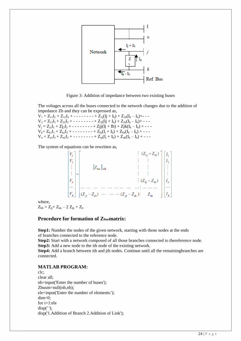
Type 4 Modification: In this type of modification, an impedance Zb is added between two existing buses j and k asshown

in Figure 3. From Figure 3, the relation between the voltages of bus k and j can be writtenas,

Vk – Vj= IbZb

24 | P a g e

Figure 3: Addition of impedance between two existing buses

The voltages across all the buses connected to the network changes due to the addition of

impedance Zb and they can be expressed as,

V1 = Z11I1 + Z12I2 + - - - - - - - - + Z1j(Ij + Ib) + Z1k(Ik – Ib)+- - -

V2 = Z21I1 + Z22I2 + - - - - - - - - + Z2j(Ij + Ib) + Z2k(Ik – Ib)+ - - -

Vj = Zj1I1 + Zj2I2 + - - - - - - - - + Zjj(Ij + Ib) + Zjk(Ik – Ib) + - - -

Vk= Zk1I1 + Zk2I2 + - - - - - - - - + Zkj(Ij + Ib) + Zkk(Ik – Ib) + - - -

Vn = Zn1I1 + Zn2I2 + - - - - - - - - + Znj(Ij + Ib) + Znk(Ik – Ib) + - - -

The system of equations can be rewritten as,

where,

Zbb = Zjj+ Zkk – 2 Zjk + Zb

Procedure for formation of Zbusmatrix:

Step1: Number the nodes of the given network, starting with those nodes at the ends

of branches connected to the reference node.

Step2: Start with a network composed of all those branches connected to thereference node.

Step3: Add a new node to the ith node of the existing network.

Step4: Add a branch between ith and jth nodes. Continue until all the remainingbranches are

connected.

MATLAB PROGRAM: clc;

clear all;

nb=input('Enter the number of buses');

Zbusm=null(nb,nb);

ele=input('Enter the number of elements:');

dim=0;

for i=1:ele

disp(' ');

disp('1.Addition of Branch 2.Addition of Link');

25 | P a g e

ch=input('Enter your choice:');

p=input('enter p value');

q=input('enter q value');

val=input('Enter value to be added;');

switch(ch)

case 1

dim=dim+1;

if p==0||q==0

for row=1:dim

for col=1:dim

Zbusm(dim,dim)=val;

Zbusm(dim+1:end,dim+1:end)=0;

end;

end;

else

for i=1:dim

Zbusm(q,i)=Zbusm(p,i);

Zbusm(i,q)=Zbusm(q,i);

end;

Zbusm(q,q)=Zbusm(p,q)+val;

end;

%end;

case 2

Zbusrm=null(dim,dim);

li=dim+1;

if p==0

for i=1:li

Zbusm(li,i)=-Zbusm(q,i);

Zbusm(i,li)=Zbusm(li,i);

end;

%end

Zbusm(li,li)=-Zbusm(q,li)+val;

else

for i=1:li

Zbusm(li,i)=Zbusm(p,i)-Zbusm(q,i);

Zbusm(i,li)=Zbusm(li,i);

end;

Zbusm(li,li)=Zbusm(p,li)-Zbusm(q,li)+val

for i=1:dim

for j=1:dim

Zbusrm(i,j)=Zbusm(i,j)-(((Zbusm(i,li))*Zbusm(li,j))/Zbusm(li,li));

end;

end;

disp(Zbusrm);

Zbusm=Zbusrm

end;

end;

end

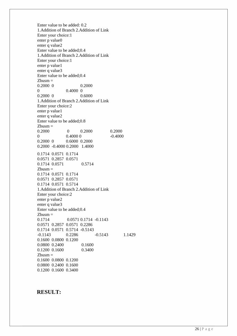
OUTPUT: Enter the number of buses: 3

Enter the number of elements:5

1. Addition of Branch 2.Addition of Link

Enter your choice:1

enter p value0

enter q value1

26 | P a g e

Enter value to be added: 0.2

1.Addition of Branch 2.Addition of Link

Enter your choice:1

enter p value0

enter q value2

Enter value to be added;0.4


Enter your choice:1

enter p value1

enter q value3


Zbusm =

0.2000 0 0.2000

0 0.4000 0

0.2000 0 0.6000


Enter your choice:2

enter p value1

enter q value2


Zbusm =

0.2000 0 0.2000 0.2000

0 0.4000 0 -0.4000

0.2000 0 0.6000 0.2000

0.2000 -0.4000 0.2000 1.4000

0.1714 0.0571 0.1714

0.0571 0.2857 0.0571

0.1714 0.0571 0.5714

Zbusm =

0.1714 0.0571 0.1714

0.0571 0.2857 0.0571

0.1714 0.0571 0.5714


Enter your choice:2

enter p value2

enter q value3


Zbusm =

0.1714 0.0571 0.1714 -0.1143

0.0571 0.2857 0.0571 0.2286

0.1714 0.0571 0.5714 -0.5143

-0.1143 0.2286 -0.5143 1.1429

0.1600 0.0800 0.1200

0.0800 0.2400 0.1600

0.1200 0.1600 0.3400

Zbusm =

0.1600 0.0800 0.1200

0.0800 0.2400 0.1600

0.1200 0.1600 0.3400

RESULT:

27 | P a g e

LAB VIVA QUESTIONS:

1. What are the diagonal elements of bus impedance matrix called?

2. When a branch of impedance Zb is added from a new bus to the reference bus, what will be the order

of the bus impedance matrix?

3. What are the off diagonal elements in Ybus called?

LAB ASSIGNMENTS:

28 | P a g e

EXPERIMENT - 8

SHORT CIRCUIT ANALYSIS

8.1 AIM:

To develop program for short circuit analysis using ZBUS algorithm

8.2 APPARATUS:


8.3 THEORY:

A fault in a circuit is a failure that interferes with the normal flow of current. A short circuit fault

occurs when the insulation of the system fails resulting in low impedance path either between phases

or phase(s) to ground. This causes excessively high currents to flow in the circuit, requiring the

operation of protective equipment to prevent damage to equipment.

The short circuit faults can be classified as:

• Symmetrical faults

• Unsymmetrical faults

A three phase symmetrical fault is caused by application of three equal fault impedances Z¯ f to the

three phases.

Faults in which the balanced state of the network is disturbed are called unsymmetrical or

unbalanced faults. The most common type of unbalanced fault in a system is a single line to ground

fault (LG fault). Almost 60 to 75% of faults in a system are LG faults. The other types of

unbalanced faults are line to line faults (LL faults) and double line to ground faults (LLG faults).

About 15 to 25% faults are LLG faults and 5 to 15% are LL faults.

29 | P a g e

ALGORITHM:

Step 1: Obtain pre-fault voltages at all buses and currents in all lines through a load flow study.

0

0

2

0

1

0

n

BUS

V

V

V

V

Ifrth

bus is faulted through a fault impedance,Zf,the post fault bus voltage is given by

VVV BUS

f

BUS 0

where ΔV is the vector of changes in bus voltages caused by the fault.

Step 2:The Thevenin network of the system with generators replaced by transient /subtransient

reactance with their emfs shorted.

Step 3: Excite the passive Thevenin networkwith –Vr0 in series with Zf. ΔV is given as

f

BUS JZV

Where,

Bus impedance matrix of the passive Thevinin network is,

nnn

n

BUSZZ

ZZZ

1

111][ and

Jf = Bus current injection vector

The current, -Ifis injected at the rth bus,

0

|

0

][

ff

rfII

J

Forrthbus,

f

rrr IZV

Step 4: The voltage at the rthbus under fault is

f

rr

o

rr

o

r

f

r IZVVVV 0

f

rr

f

r IZV

f

rr

o

r

ff IZVIZ

f

rr

o

rf

ZZ

VI

0

rf

rr

iro

i

f

i VZZ

ZVV

ZBUS matrix is obtained byZBUSbuilding algorithm.

30 | P a g e

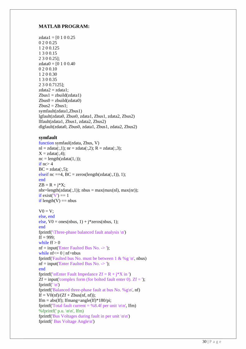
MATLAB PROGRAM:

zdata1 = [0 1 0 0.25

0 2 0 0.25

1 2 0 0.125

1 3 0 0.15

2 3 0 0.25];

zdata0 = [0 1 0 0.40

0 2 0 0.10

1 2 0 0.30

1 3 0 0.35

2 3 0 0.7125];

zdata2 = zdata1;

Zbus1 = zbuild(zdata1)

Zbus0 = zbuild(zdata0)

Zbus2 = Zbus1;

symfault(zdata1,Zbus1)

lgfault(zdata0, Zbus0, zdata1, Zbus1, zdata2, Zbus2)

llfault(zdata1, Zbus1, zdata2, Zbus2)

dlgfault(zdata0, Zbus0, zdata1, Zbus1, zdata2, Zbus2)

symfault function symfaul(zdata, Zbus, V)

nl = zdata(:,1); nr = zdata(:,2); R = zdata(:,3);

X = zdata(:,4);

nc = length(zdata(1,:));

if nc> 4

BC = zdata(:,5);

elseif nc ==4, BC = zeros(length(zdata(:,1)), 1);

end

ZB = R + j*X;

nbr=length(zdata(:,1)); nbus = max(max(nl), max(nr));

if exist('V') == 1

if length(V) == nbus

V0 = V;

else, end

else, V0 = ones(nbus, 1) + j*zeros(nbus, 1);

end

fprintf('\Three-phase balanced fault analysis \n')

ff = 999;

while ff > 0

nf = input('Enter Faulted Bus No. -> ');

while nf<= 0 | nf>nbus

fprintf('Faulted bus No. must be between 1 & %g \n', nbus)


end

fprintf('\nEnter Fault Impedance Zf = R + j*X in ')

Zf = input('complex form (for bolted fault enter 0). Zf = ');

fprintf(' \n')

fprintf('Balanced three-phase fault at bus No. %g\n', nf)

If = V0(nf)/(Zf + Zbus(nf, nf));

Ifm = abs(If); Ifmang=angle(If)*180/pi;

fprintf('Total fault current = %8.4f per unit \n\n', Ifm)

%fprintf(' p.u. \n\n', Ifm)

fprintf('Bus Voltages during fault in per unit \n\n')

fprintf(' Bus Voltage Angle\n')

31 | P a g e

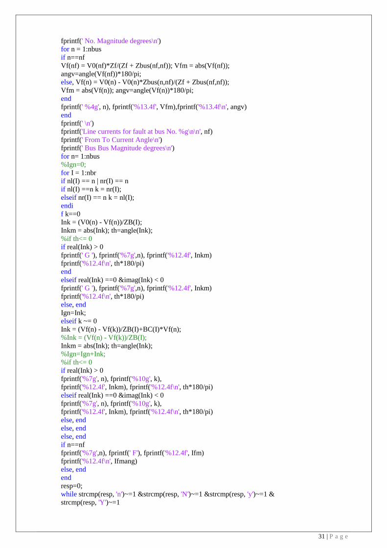
fprintf(' No. Magnitude degrees\n')

for n = 1:nbus

if n==nf

Vf(nf) = V0(nf)*Zf/(Zf + Zbus(nf,nf)); Vfm = abs(Vf(nf));

angv=angle(Vf(nf))*180/pi;

else, Vf(n) = V0(n) - V0(n)*Zbus(n,nf)/(Zf + Zbus(nf,nf));

Vfm = abs(Vf(n)); angv=angle(Vf(n))*180/pi;

end

fprintf(' %4g', n), fprintf('%13.4f', Vfm),fprintf('%13.4f\n', angv)

end

fprintf(' \n')

fprintf('Line currents for fault at bus No. %g\n\n', nf)

fprintf(' From To Current Angle\n')

fprintf(' Bus Bus Magnitude degrees\n')

for n= 1:nbus

%Ign=0;

for I = 1:nbr

if nl(I) == n | nr(I) == n

if nl(I) ==n k = nr(I);

elseif nr(I) == n k = nl(I);

endi

f k==0

Ink = (V0(n) - Vf(n))/ZB(I);

Inkm = abs(Ink); th=angle(Ink);

%if th<= 0

if real(Ink) > 0

fprintf(' G '), fprintf('%7g',n), fprintf('%12.4f', Inkm)

fprintf('%12.4f\n', th*180/pi)

end

elseif real(Ink) ==0 &imag(Ink) < 0

fprintf(' G '), fprintf('%7g',n), fprintf('%12.4f', Inkm)

fprintf('%12.4f\n', th*180/pi)

else, end

Ign=Ink;

elseif k ~= 0

Ink = (Vf(n) - Vf(k))/ZB(I)+BC(I)*Vf(n);

%Ink = (Vf(n) - Vf(k))/ZB(I);

Inkm = abs(Ink); th=angle(Ink);

%Ign=Ign+Ink;

%if th<= 0

if real(Ink) > 0

fprintf('%7g', n), fprintf('%10g', k),

fprintf('%12.4f', Inkm), fprintf('%12.4f\n', th*180/pi)

elseif real(Ink) ==0 &imag(Ink) < 0


fprintf('%12.4f', Inkm), fprintf('%12.4f\n', th*180/pi)

else, end

else, end

else, end

if n==nf

fprintf('%7g',n), fprintf(' F'), fprintf('%12.4f', Ifm)

fprintf('%12.4f\n', Ifmang)

else, end

end

resp=0;

while strcmp(resp, 'n')~=1 &strcmp(resp, 'N')~=1 &strcmp(resp, 'y')~=1 &

strcmp(resp, 'Y')~=1

32 | P a g e

resp = input('Another fault location? Enter ''y'' or ''n'' within single quote-> ');

if strcmp(resp, 'n')~=1 &strcmp(resp, 'N')~=1 &strcmp(resp, 'y')~=1 &


fprintf('\n Incorrect reply, try again \n\n'), end

end

if resp == 'y' | resp == 'Y'

nf = 999;

else ff = 0; end

end % end for while

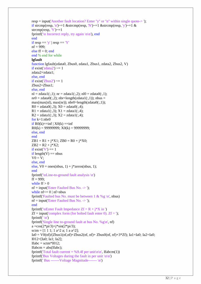
lgfault

function lgfault(zdata0, Zbus0, zdata1, Zbus1, zdata2, Zbus2, V)

if exist('zdata2') ~= 1

zdata2=zdata1;

else, end

if exist('Zbus2') ~= 1

Zbus2=Zbus1;

else, end

nl = zdata1(:,1); nr = zdata1(:,2); nl0 = zdata0(:,1);

nr0 = zdata0(:,2); nbr=length(zdata1(:,1)); nbus =

max(max(nl), max(nr)); nbr0=length(zdata0(:,1));

R0 = zdata0(:,3); X0 = zdata0(:,4);

R1 = zdata1(:,3); X1 = zdata1(:,4);

R2 = zdata1(:,3); X2 = zdata1(:,4);

for k=1:nbr0

if R0(k)==inf | X0(k) ==inf

R0(k) = 99999999; X0(k) = 99999999;

else, end

end

ZB1 = R1 + j*X1; ZB0 = R0 + j*X0;

ZB2 = R2 + j*X2;

if exist('V') == 1


V0 = V;

else, end


end

fprintf('\nLine-to-ground fault analysis \n')

ff = 999;

while ff > 0





end



fprintf(' \n')

fprintf('Single line to-ground fault at bus No. %g\n', nf)

a =cos(2*pi/3)+j*sin(2*pi/3);

sctm = [1 1 1; 1 a^2 a; 1 a a^2];

Ia0 = V0(nf)/(Zbus1(nf,nf)+Zbus2(nf, nf)+ Zbus0(nf, nf)+3*Zf); Ia1=Ia0; Ia2=Ia0;

I012=[Ia0; Ia1; Ia2];

Ifabc = sctm*I012;

Ifabcm = abs(Ifabc);

fprintf('Total fault current = %9.4f per unit\n\n', Ifabcm(1))

fprintf('Bus Voltages during the fault in per unit \n\n')

fprintf(' Bus -------Voltage Magnitude------- \n')

33 | P a g e

fprintf(' No. Phase a Phase b Phase c \n')

for n = 1:nbus

Vf0(n)= 0 - Zbus0(n, nf)*Ia0;

Vf1(n)= V0(n) - Zbus1(n, nf)*Ia1;


Vabc = sctm*[Vf0(n); Vf1(n); Vf2(n)];

Va(n)=Vabc(1); Vb(n)=Vabc(2); Vc(n)=Vabc(3);

fprintf(' %5g',n)

fprintf(' %11.4f', abs(Va(n))),fprintf(' %11.4f', abs(Vb(n)))

fprintf(' %11.4f\n', abs(Vc(n)))

end

fprintf(' \n')


fprintf(' From To -----Line Current Magnitude---- \n')

fprintf(' Bus Bus Phase a Phase b Phase c \n')

for n= 1:nbus

for I = 1:nbr

if nl(I) == n | nr(I) == n



end

end

if k ~= 0

Ink1(n, k) = (Vf1(n) - Vf1(k))/ZB1(I);

Ink2(n, k) = (Vf2(n) - Vf2(k))/ZB2(I);

else, end

else, end

for I = 1:nbr0

if nl0(I) == n | nr0(I) == n

if nl0(I) ==n k = nr0(I);

elseif nr0(I) == n k = nl0(I);

end

end

if k ~= 0

Ink0(n, k) = (Vf0(n) - Vf0(k))/ZB0(I);

else, end

else, end

for I = 1:nbr

if nl(I) == n | nr(I) == n



end

if k ~= 0

Inkabc = sctm*[Ink0(n, k); Ink1(n, k); Ink2(n, k)];

Inkabcm = abs(Inkabc); th=angle(Inkabc);

if real(Inkabc(1)) > 0


fprintf(' %11.4f', abs(Inkabc(1))),fprintf(' %11.4f',

abs(Inkabc(2)))

abs(Inkabc(2)))

fprintf(' %11.4f\n', abs(Inkabc(3)))

elseif real(Inkabc(1)) ==0 &imag(Inkabc(1)) < 0




else, end

end

34 | P a g e

else, end

else, end

end

if n==nf

fprintf('%7g',n), fprintf(' F'),

fprintf(' %11.4f', Ifabcm(1)),fprintf(' %11.4f', Ifabcm(2))

fprintf(' %11.4f\n', Ifabcm(3))

else, end

resp=0;



resp = input('Another fault location? Enter ''y'' or ''n'' within single quote-> ');




end


nf = 999;

else ff = 0; end

end % end for while

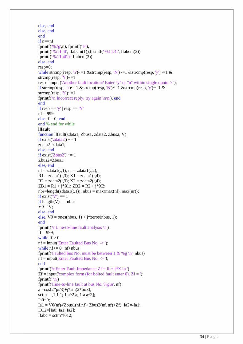
llfault

function llfault(zdata1, Zbus1, zdata2, Zbus2, V)


zdata2=zdata1;

else, end


Zbus2=Zbus1;

else, end

nl = zdata1(:,1); nr = zdata1(:,2);

R1 = zdata1(:,3); X1 = zdata1(:,4);

R2 = zdata2(:,3); X2 = zdata2(:,4);

ZB1 = R1 + j*X1; ZB2 = R2 + j*X2;

nbr=length(zdata1(:,1)); nbus = max(max(nl), max(nr));

if exist(' V') == 1


V0 = V;

else, end


end

fprintf('\nLine-to-line fault analysis \n')

ff = 999;

while ff > 0





end



fprintf(' \n')

fprintf('Line-to-line fault at bus No. %g\n', nf)


sctm = [1 1 1; 1 a^2 a; 1 a a^2];

Ia0=0;

Ia1 = V0(nf)/(Zbus1(nf,nf)+Zbus2(nf, nf)+Zf); Ia2=-Ia1;

I012=[Ia0; Ia1; Ia2];

Ifabc = sctm*I012;

35 | P a g e

Ifabcm = abs(Ifabc);

fprintf('Total fault current = %9.4f per unit\n\n', Ifabcm(2))




for n = 1:nbus

Vf0(n)= 0;





fprintf(' %5g',n)



end

fprintf(' \n')




for n= 1:nbus

for I = 1:nbr

if nl(I) == n | nr(I) == n



end

if k ~= 0

Ink0(n, k) = 0;

Ink1(n, k) = (Vf1(n) - Vf1(k))/ZB1(I);

Ink2(n, k) = (Vf2(n) - Vf2(k))/ZB2(I);



if real(Inkabc(2)) < 0

abs(Inkabc(2)))

abs(Inkabc(2)))




elseif real(Inkabc(2)) ==0 &imag(Inkabc(2)) > 0




else, end

end

else, end

else, end

end

if n==nf




else, end

resp=0;



resp = input('Another fault location? Enter ''y'' or ''n'' within single quote

-> ');

36 | P a g e




end


nf = 999;

else ff = 0; end

end % end for while

dlgfault

function dlgfault(zdata0, Zbus0, zdata1, Zbus1, zdata2, Zbus2, V)


zdata2=zdata1;

else, end


Zbus2=Zbus1;

else, end

nl = zdata1(:,1); nr = zdata1(:,2); nl0 = zdata0(:,1);

nr0 = zdata0(:,2); nbr=length(zdata1(:,1)); nbus =

max(max(nl), max(nr)); nbr0=length(zdata0(:,1));

R0 = zdata0(:,3); X0 = zdata0(:,4);

R1 = zdata1(:,3); X1 = zdata1(:,4);

R2 = zdata2(:,3); X2 = zdata2(:,4);

for k = 1:nbr0

if R0(k) == inf | X0(k) == inf

R0(k) = 99999999; X0(k) = 999999999;

else, end

end

ZB1 = R1 + j*X1; ZB0 = R0 + j*X0;

ZB2 = R2 + j*X2;

if exist('V') == 1


V0 = V;

else, end


end

fprintf('\nDouble line-to-ground fault analysis \n')

ff = 999;

while ff > 0





end



fprintf(' \n')

fprintf('Double line-to-ground fault at bus No. %g\n', nf)


sctm = [1 1 1; 1 a^2 a; 1 a a^2];

Z11 = Zbus2(nf, nf)*(Zbus0(nf, nf)+ 3*Zf)/(Zbus2(nf, nf)+Zbus0(nf, nf)+3*Zf);

Ia1 = V0(nf)/(Zbus1(nf,nf)+Z11);

Ia2 =-(V0(nf) - Zbus1(nf, nf)*Ia1)/Zbus2(nf,nf);

Ia0 =-(V0(nf) - Zbus1(nf, nf)*Ia1)/(Zbus0(nf,nf)+3*Zf);

I012=[Ia0; Ia1; Ia2];

Ifabc = sctm*I012; Ifabcm=abs(Ifabc);

37 | P a g e

Ift = Ifabc(2)+Ifabc(3);

Iftm = abs(Ift);

fprintf('Total fault current = %9.4f per unit\n\n', Iftm)




for n = 1:nbus






fprintf(' %5g',n)



end

fprintf(' \n')




for n= 1:nbus

for I = 1:nbr

if nl(I) == n | nr(I) == n



end

end

if k ~= 0

Ink1(n, k) = (Vf1(n) - Vf1(k))/ZB1(I);

Ink2(n, k) = (Vf2(n) - Vf2(k))/ZB2(I);

else, end

else, end

for I = 1:nbr0

if nl0(I) == n | nr0(I) == n

if nl0(I) ==n k = nr0(I);

elseif nr0(I) == n k = nl0(I);

end

end

if k ~= 0

Ink0(n, k) = (Vf0(n) - Vf0(k))/ZB0(I);

else, end

else, end

for I = 1:nbr

if nl(I) == n | nr(I) == n



end

if k ~= 0



if real(Inkabc(2)) < 0

abs(Inkabc(2)))

abs(Inkabc(2)))




38 | P a g e

elseif real(Inkabc(2)) ==0 &imag(Inkabc(2)) > 0




else, end

end

else, end

else, end

end

if n==nf




else, end

resp=0;



resp = input('Another fault location? Enter ''y'' or ''n'' within single quote

-> ');




end


nf = 999;

else ff = 0; end

end % end for while

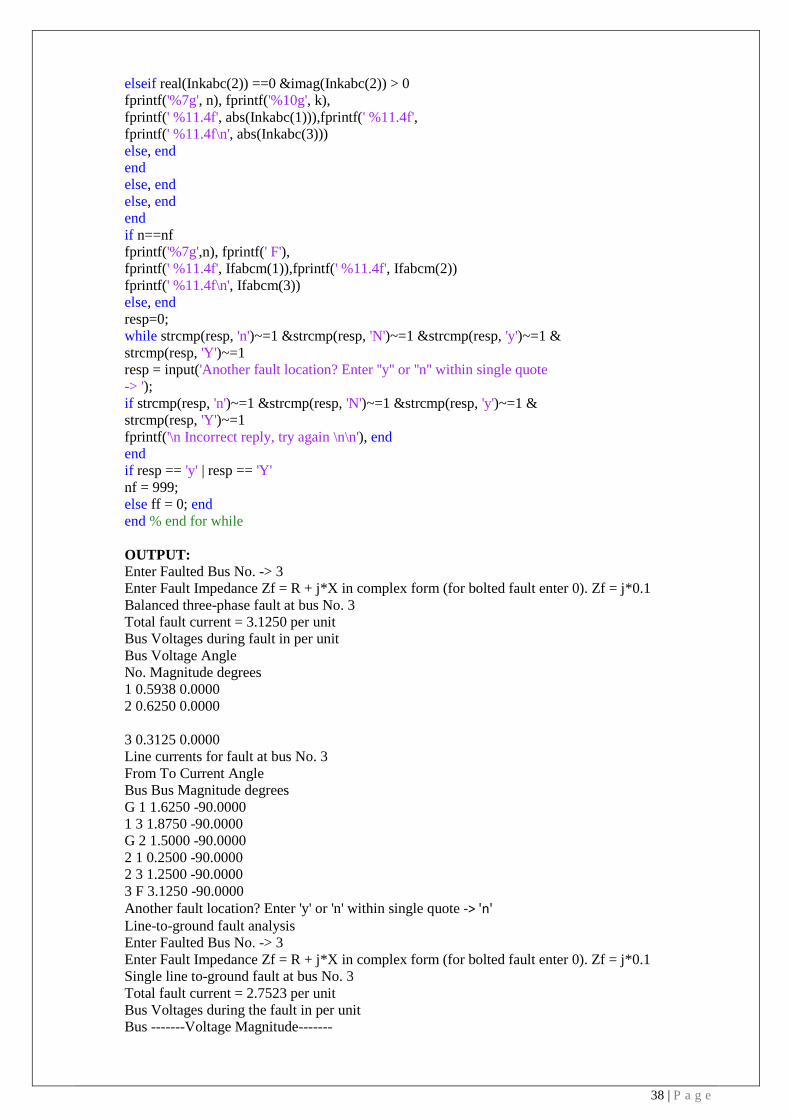
OUTPUT:

Enter Faulted Bus No. -> 3

Enter Fault Impedance Zf = R + j*X in complex form (for bolted fault enter 0). Zf = j*0.1

Balanced three-phase fault at bus No. 3

Total fault current = 3.1250 per unit

Bus Voltages during fault in per unit

Bus Voltage Angle

No. Magnitude degrees

1 0.5938 0.0000

2 0.6250 0.0000

3 0.3125 0.0000

Line currents for fault at bus No. 3

From To Current Angle

Bus Bus Magnitude degrees

G 1 1.6250 -90.0000

1 3 1.8750 -90.0000

G 2 1.5000 -90.0000

2 1 0.2500 -90.0000

2 3 1.2500 -90.0000

3 F 3.1250 -90.0000

Another fault location? Enter 'y' or 'n' within single quote -> 'n' Line-to-ground fault analysis



Single line to-ground fault at bus No. 3


Bus Voltages during the fault in per unit

Bus -------Voltage Magnitude-------

39 | P a g e

No. Phase a Phase b Phase c

1 0.6330 1.0046 1.0046

2 0.7202 0.9757 0.9757

3 0.2752 1.0647 1.0647


From To -----Line Current Magnitude----

Bus Bus Phase a Phase b Phase c

95 1 3 1.6514 0.0000 0.0000

2 1 0.3761 0.1560 0.1560

2 3 1.1009 0.0000 0.0000

3 F 2.7523 0.0000 0.0000

Another fault location? Enter 'y' or 'n' within single quote -> 'n'

Line-to-line fault analysis



Line-to-line fault at bus No. 3





1 1.0000 0.6720 0.6720

2 1.0000 0.6939 0.6939

3 1.0000 0.5251 0.5251




1 3 0.0000 1.9245 1.9245

2 1 0.0000 0.2566 0.2566

2 3 0.0000 1.2830 1.2830

3 F 0.0000 3.2075 3.2075


Double line-to-ground fault analysis



Double line-to-ground fault at bus No. 3





1 1.0066 0.5088 0.5088

2 0.9638 0.5740 0.5740

3 1.0855 0.1974 0.1974




1 3 0.0000 2.4350 2.4350

2 1 0.1118 0.3682 0.3682

2 3 0.0000 1.6233 1.6233

3 F 0.0000 4.0583 4.0583


RESULT:

40 | P a g e

LAB VIVA QUESTIONS:

1. What percentage of fault occurring in the power system is LLG fault?

2. What percentage of fault occurring in the power system is line to line fault?

3. What are the types of unsymmetrical faults?

4. Which is the most severe fault?

5. In which portion of the transmission system is the occurrence of the fault more common?

6. Which is the most commonly occurring fault?

LAB ASSIGNMENTS:

41 | P a g e

EXPERIMENT - 9

TRANSIENT STABILITY

9.1 AIM:

To develop program for transient stability analysis for single machine connected to infinitebus

9.2 APPARATUS:


9.3 THEORY:

Stability: Stability problem is concerned with the behavior of power system when it is subjected

todisturbance and is classified into small signal stability problem if the disturbances are small

andtransient stability problem when the disturbances are large.

Transient stability: When a power system is under steady state, the load plus transmission loss

equals to the generation in the system. The generating units run a synchronous speed and system

frequency, voltage, current and power flows are steady. When a large disturbance such as three

phase fault, loss of load, loss of generation etc., occurs the power balance is upset and the generating

units rotors experience either acceleration or deceleration. The system may come back to a steady

state condition maintaining synchronism or it may break into subsystems or one or more machines

may pull out of synchronism. In the former case the system is said to be stable and in the later case it

is said to be unstable.

Reactive power Qe = sin(cos-1

(p.f))

Stator current, It=S*/Et*

= Pe-jQe/Et*

Voltage behind transient condition

Voltage of infinite bus

Angular separation between E1 and EB

Pre-fault Operation:

42 | P a g e

During Fault Condition:

Find out X from the equivalent circuit during fault condition

Post fault Condition: Find out X from the equivalent circuit during post fault condition

Critical Clearing Angle:

43 | P a g e

Critical Clearing Time:

MATLAB PROGRAM:

a) Pm = 0.8; E = 1.17; V = 1.0;

X1 = 0.65; X2 = inf; X3 = 0.65;

eacfault(Pm, E, V, X1, X2, X3)

b) Pm = 0.8; E = 1.17; V = 1.0;

X1 = 0.65; X2 = 1.8; X3 = 0.8;

eacfault(Pm, E, V, X1, X2, X3)

eacfault

function eacfault(Pm, E, V, X1, X2, X3)

if exist('Pm')~=1

Pm = input('Generator output power in p.u. Pm = '); else, end

if exist('E')~=1

E = input('Generator e.m.f. in p.u. E = '); else, end

if exist('V')~=1

V = input('Infinite bus-bar voltage in p.u. V = '); else, end

if exist('X1')~=1

X1 = input('Reactance before Fault in p.u. X1 = '); else, end

if exist('X2')~=1

X2 = input('Reactance during Fault in p.u. X2 = '); else, end

if exist('X3')~=1

X3 = input('Reactance aftere Fault in p.u. X3 = '); else, end

Pe1max = E*V/X1; Pe2max=E*V/X2; Pe3max=E*V/X3;

delta = 0:.01:pi;

Pe1 = Pe1max*sin(delta); Pe2 = Pe2max*sin(delta); Pe3 = Pe3max*sin(delta);

d0 =asin(Pm/Pe1max); dmax = pi-asin(Pm/Pe3max);

cosdc = (Pm*(dmax-d0)+Pe3max*cos(dmax)-Pe2max*cos(d0))/(Pe3max-Pe2max);

if abs(cosdc) > 1

fprintf('No critical clearing angle could be found.\n')

fprintf('system can remain stable during this disturbance.\n\n')

return

else, end

dc=acos(cosdc);

if dc >dmax

fprintf('No critical clearing angle could be found.\n')

fprintf('System can remain stable during this disturbance.\n\n')

return

else, end

Pmx=[0 pi-d0]*180/pi; Pmy=[Pm Pm];

x0=[d0 d0]*180/pi; y0=[0 Pm]; xc=[dc dc]*180/pi; yc=[0 Pe3max*sin(dc)];

xm=[dmaxdmax]*180/pi; ym=[0 Pe3max*sin(dmax)];

d0=d0*180/pi; dmax=dmax*180/pi; dc=dc*180/pi;

x=(d0:.1:dc);

y=Pe2max*sin(x*pi/180);

y1=Pe2max*sin(d0*pi/180);

y2=Pe2max*sin(dc*pi/180);

44 | P a g e

x=[d0 x dc];

y=[Pm y Pm];

xx=dc:.1:dmax;

h=Pe3max*sin(xx*pi/180);

xx=[dc xx dmax];

hh=[Pm h Pm];

delta=delta*180/pi;

if X2 == inf

fprintf('\nFor this case tc can be found from analytical formula. \n')

H=input('To find tc enter Inertia Constant H, (or 0 to skip) H = ');

if H ~= 0

d0r=d0*pi/180; dcr=dc*pi/180;

tc = sqrt(2*H*(dcr-d0r)/(pi*60*Pm));

else, end

else, end

%clc

fprintf('\nInitial power angle = %7.3f \n', d0)

fprintf('Maximum angle swing = %7.3f \n', dmax)

fprintf('Critical clearing angle = %7.3f \n\n', dc)

if X2==inf & H~=0

fprintf('Critical clearing time = %7.3f sec. \n\n', tc)

else, end

h = figure; figure(h);

fill(x,y,'m')

hold;

fill(xx,hh,'c')

plot(delta, Pe1,'-', delta, Pe2,'r-', delta, Pe3,'g-', Pmx, Pmy,'b-', x0,y0,

xc,yc, xm,ym), grid

Title('Application of equal area criterion to a critically cleared system')

xlabel('Power angle, degree'), ylabel(' Power, per unit')

text(5, 1.07*Pm, 'Pm')

text(50, 1.05*Pe1max,['Critical clearing angle = ',num2str(dc)])

axis([0 180 0 1.1*Pe1max])

hold off;

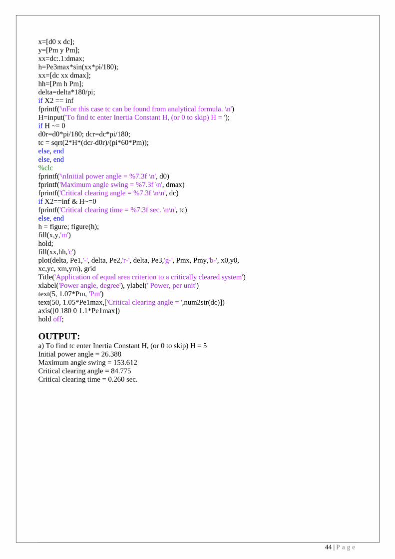
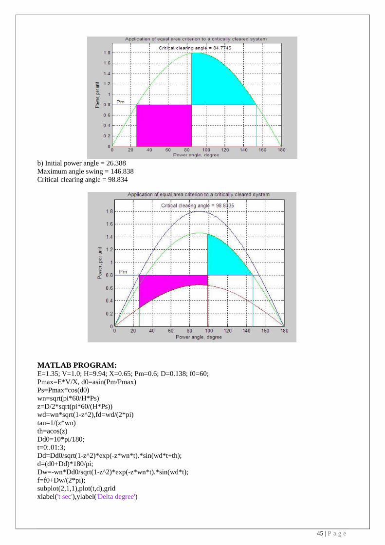
OUTPUT: a) To find tc enter Inertia Constant H, (or 0 to skip) H = 5

Initial power angle = 26.388

Maximum angle swing = 153.612

Critical clearing angle = 84.775

Critical clearing time = 0.260 sec.

45 | P a g e

b) Initial power angle = 26.388

Maximum angle swing = 146.838

Critical clearing angle = 98.834

MATLAB PROGRAM: E=1.35; V=1.0; H=9.94; X=0.65; Pm=0.6; D=0.138; f0=60;

Pmax=E*V/X, d0=asin(Pm/Pmax)

Ps=Pmax*cos(d0)

wn=sqrt(pi*60/H*Ps)

z=D/2*sqrt(pi*60/(H*Ps))

wd=wn*sqrt(1-z^2),fd=wd/(2*pi)

tau=1/(z*wn)

th=acos(z)

Dd0=10*pi/180;

t=0:.01:3;

Dd=Dd0/sqrt(1-z^2)*exp(-z*wn*t).*sin(wd*t+th);

d=(d0+Dd)*180/pi;

Dw=-wn*Dd0/sqrt(1-z^2)*exp(-z*wn*t).*sin(wd*t);

f=f0+Dw/(2*pi);

subplot(2,1,1),plot(t,d),grid

xlabel('t sec'),ylabel('Delta degree')

46 | P a g e

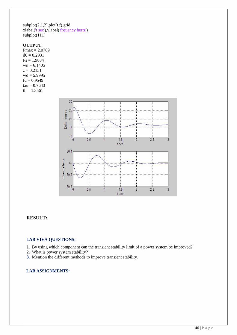
subplot(2,1,2),plot(t,f),grid

xlabel('t sec'),ylabel('frquency hertz')

subplot(111)

OUTPUT:

Pmax = 2.0769

d0 = 0.2931

Ps = 1.9884

wn = 6.1405

z = 0.2131

wd = 5.9995

fd = 0.9549

tau = 0.7643

th = 1.3561

RESULT:

LAB VIVA QUESTIONS:

1. By using which component can the transient stability limit of a power system be improved?

2. What is power system stability?

3. Mention the different methods to improve transient stability.

LAB ASSIGNMENTS:

47 | P a g e

EXPERIMENT - 10

LOAD DISPATCH PROBLEM

10.1 AIM:

To develop program for economic load dispatch problem using lambda iterative method

10.2 APPARATUS:


10.3 THEORY:

A modern power system is invariably fed from a number of power plants. Research and

development has led to efficient power plant equipment. A generating unit added to the systemtoday

is likely to be more efficient than the one added some time back. With a very large numberof

generating units at hand, it is the job of the operating engineers to allocate the loads betweenthe

units such that the operating costs are the minimum. The optimal load allocation is byconsidering a

system with any number of units. The loads should be so allocated among thedifferent units that

every unit operates at the same incremental cost. This criterion can bedeveloped mathematically by

the method of lagrangian multiplier.

Statement of Economic Dispatch Problem: In a power system, with negligible transmission losses and with N number of spinning thermal

generating units the total system load PD at a particular interval can be met by different sets of

generation schedules.

PG1(K)

, PG2(K)

,…… . . PGN(K)

k =1,2,……….NS

Out of these NS sets of generation schedules, the system operator has to choose that setof schedule

which minimizes the system operating cost which is essentially the sum of theproduction costs of all

the generating units. This economic dispatch problem is mathematicallystated as an optimization

problem. Given the number of available generating units Ns theirproduction cost function, their

operating limits and the system load PD.

To determine the set of generating schedule PG,

Min FT = Fi . PGi Ni (1)

where𝐹𝑖 . 𝑃𝐺𝑖 = 𝑎𝑖 𝑃𝐺𝑖2 + 𝑏𝑖𝑃𝐺𝑖 + 𝑐𝑖 i=1,2……N (2)

Φ= 𝑃𝐺𝑖𝑁𝑖 − 𝑃𝐷=0 (3)

𝑃𝐺𝑖 𝑚𝑖𝑛 ≤ 𝑃𝐺𝑖 ≤ 𝑃𝐺𝑖𝑚𝑎𝑥 (4)

where ai, bi and ci are constants.

The ED problem is given by the equations (1) to (3). By omitting the inequality constraint

thereduced ED problem may be restated as an unconstrained optimization problem by augmenting

the objective function with the constraint function Φ multiplied by Lagrange multiplier λ to obtain

the Lagrange function L as,

(5)

(6)

(7) The solution to ED problem can be obtained by solving simultaneously the necessary conditions(6)

and (7) which state that the economic generation schedules not only satisfy the system powerbalance

48 | P a g e

equation (8) but also demand that the incremental cost rates of all the units be equal to λwhich can

be interpreted as “incremental cost of received power” when the inequality constraints(3) are

included in the ED problem the necessary condition (6) gets modified as

(8)

The solution to the ED problem with the production cost function assumed to be a

quadraticfunction, equation (4), can be obtained by simultaneously solving (6) and (7) using a

directmethod as given below,

(9)

(10)

Substituting Equation (10) in Equation (7) we obtain

(11)

The method of solution involves computing λ using equation (11) and then computing theeconomic

schedules PGi; i=1,2,........N using equation (10). In order to satisfy the operating limits(3) the

following iterative algorithm is to be used.

ALGORITHM:

Step 1: Choose appropriate value of Lagrangian multiplier λ

Step 2: Start iteration iter=0

Step 3: Iteration iter=iter+1

Step 4: Solve for power generated by ith unit using equation

Step 5: Check if any Pi is beyond or below the inequality constant

If Pi <Pi,min, fix Pi= Pi,min

If Pi>Pi,max, fix Pi= Pi,max

Step 6: Calculate the power loss using the equation

Step 7: Calculate power mismatch using the formula,

Step 8: If , then increment λ, λnew=λ+0.001 and go to step 3else go to step 9

Step 9: If , then decrement λ, λnew=λ-0.001 and go to step 3else go to step 10

Step 10:If ΔP is less than tolerance value , print the values of generatedpower and losses

Step11:Stop

MATLAB Program:

clc;

clear all; % a b c fc max min

49 | P a g e

data= [0.00142 7.20 510 1.1 600 150

0.00194 7.85 310 1 400 100

0.00482 7.97 78 1 200 050];

ng=length(data(:,1));

a=data(:,1);

b=data(:,2);

c=data(:,3);

fc=data(:,4);

pmax=data(:,5);

pmin=data(:,6);

% loss=[0.00003 0.00009 0.00012];

loss=[ 0 0 0];

C=fc.*c; B=fc.*b; A=fc.*a;

la=1; pd=850; acc=0.2;

diff=1;

145

while acc<(abs(diff));

for i=1:ng;

p(i)= (la-B(i))/(2*(la*loss(i)+A(i)));

if p(i)<pmin(i);

p(i)=pmin(i);

end;

if p(i)>pmax(i);

p(i)=pmax(i);

end;

end;

LS=sum(((p.*p).*loss));

diff=(pd+LS-sum(p));

if diff>0

la=la+0.001;

else la=la-0.001;

end;

end;

PowerShared=p

Lambda=la

Loss=LS

OUTPUT:

a). When loss = [0.00003 0.00009 0.00012]

Power Shared = 435.1026 299.9085 130.6311

Lambda = 9.5290

Loss = 15.8222

b). When loss = 0

Power Shared = 393.0858 334.5361 122.1992

Lambda = 9.1490

Loss = 0

RESULT:

LAB VIVA QUESTIONS:

1. Define economic load disptach

2. State the objectives of economic load dispatch.

3. Name the methods of finding economic dispatch

LAB ASSIGNMENTS:

50 | P a g e

EXPERIMENT - 11

DYNAMIC PROGRAMMING METHOD

11.1 AIM:

To developprogram for unit commitment problem using forward dynamic programming method.

11.2 APPARATUS:


11.3 THEORY:

Unit commitment (UC) is an optimization problem used to determine the operation schedule of the

generating units at every hour interval with varying loads under different constraints and

environments.

In the dynamic-programming approach that follows, we assume that:

1. A state consists of an array of units with specified units operating and

2. The start-up cost of a unit is independent of the time it has been off-line

3. There are no costs for shutting down a unit.

4. There is a strict priority order, and in each interval a specified minimumamount of capacity must

be operating.

A feasible state is one in which the committed units can supply the required load and that meets the

minimum amount of capacity each period.

Flowchart:

51 | P a g e

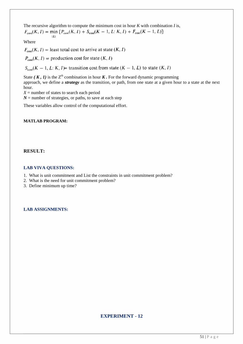
The recursive algorithm to compute the minimum cost in hour K with combination I is,

Where

State ( K , 1) is the Z

th combination in hour K . For the forward dynamic programming

approach, we define a strategy as the transition, or path, from one state at a given hour to a state at the next

hour.

X = number of states to search each period

N = number of strategies, or paths, to save at each step

These variables allow control of the computational effort.

MATLAB PROGRAM:

RESULT:

LAB VIVA QUESTIONS:

1. What is unit commitment and List the constraints in unit commitment problem?

2. What is the need for unit commitment problem?

3. Define minimum up time?

LAB ASSIGNMENTS:

EXPERIMENT - 12

52 | P a g e

EXPERIMENT - 12

STATE ESTIMATION

12.1 AIM:

To develop program for state estimation of power system.

12.2 APPARATUS:


12.3 THEORY:

Power System State Estimation is a process whereby telemetered data from network measuring

points to a central computer, can be formed into a set of reliable data for control and recording

purposes. State estimation for electric transmission grids was first formulated as a weighted least-

squares problem by Fred Schweppe and his research group in 1969.

A static state estimate is obtained from measurements taken within a time interval of about 0-5 s.

This is the commonly used state estimator. A state estimator of this type essentially gives a steady

state snapshot of the system.

A dynamic state estimate is obtained from measurements in a relatively shorter time (say 0.01 s).

Moreover, all such measurements are synchronised or "time stamped" using a common clock and

communicated from geographically distant locations to a load dispatch centre. These measurements

could be used for advanced control schemes.

The state variables of State estimation are the voltages and phase angles. Once the estimates of the

state variables are known proper actions, if required (during emergency, normal insecure states), can

be taken to bring the system back to its normal secure state.

Mathematical model:

Let the measurements, states and measurement errors be related by the nonlinear equation

Z = h(x) + p (1)

where Z is the (m x 1) measurement vector,

h(x) is the vector of nonlinear functions,

x is the (n x i) state vector,

p is the measurement error vector,

m is the number of measurements and

n the number of state variables.

A state estimate x is sought that minimizes

J(x) = ~ [z - h(x)] T w [z - h(x)] (2)

where W is a diagonal matrix whose elements are the inverses of the measurement variances.

It is assumed that E(p) = 0 and E(pvT) T = R.

The minimum of J(x) is achieved by getting an estimator of x which makes its gradient zero :

(3)

The Taylor series expansion of the nonlinear function around a nominal condition is

(4)

Substituting equation (4) into equation (3) gives

where

53 | P a g e

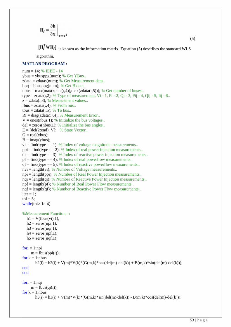
(5)

is known as the information matrix. Equation (5) describes the standard WLS

algorithm.

MATLAB PROGRAM :

num = 14; % IEEE - 14

ybus = ybusppg(num); % Get YBus..

zdata = zdatas(num); % Get Measurement data..

bpq = bbusppg(num); % Get B data..

nbus = max(max(zdata(:,4)),max(zdata(:,5))); % Get number of buses..

type = zdata(:,2); % Type of measurement, Vi - 1, Pi - 2, Qi - 3, Pij - 4, Qij - 5, Iij - 6..

z = zdata(:,3); % Measuement values..

fbus = zdata(:,4); % From bus..

tbus = zdata(:,5); % To bus..

Ri = diag(zdata(:,6)); % Measurement Error..

V = ones(nbus,1); % Initialize the bus voltages..

del = zeros(nbus,1); % Initialize the bus angles..

E = [del(2:end); V]; % State Vector..

G = real(ybus);

B = imag(ybus);

vi = find(type == 1); % Index of voltage magnitude measurements..

ppi = find(type == 2); % Index of real power injection measurements..

qi = find(type == 3); % Index of reactive power injection measurements..

pf = find(type == 4); % Index of real powerflow measurements..

qf = find(type == 5); % Index of reactive powerflow measurements..

nvi = length(vi); % Number of Voltage measurements..

npi = length(ppi); % Number of Real Power Injection measurements..

nqi = length(qi); % Number of Reactive Power Injection measurements..

npf = length(pf); % Number of Real Power Flow measurements..

nqf = length(qf); % Number of Reactive Power Flow measurements..

iter = 1;

tol = 5;

while(tol> 1e-4)

%Measurement Function, h

h1 = V(fbus(vi),1);

h2 = zeros(npi,1);

h3 = zeros(nqi,1);

h4 = zeros(npf,1);

h5 = zeros(nqf,1);

fori = 1:npi

m = fbus(ppi(i));

for k = 1:nbus

h2(i) = h2(i) + V(m)*V(k)*(G(m,k)*cos(del(m)-del(k)) + B(m,k)*sin(del(m)-del(k)));

end

end

fori = 1:nqi

m = fbus(qi(i));

for k = 1:nbus

h3(i) = h3(i) + V(m)*V(k)*(G(m,k)*sin(del(m)-del(k)) - B(m,k)*cos(del(m)-del(k)));

54 | P a g e

end

end

fori = 1:npf

m = fbus(pf(i));

n = tbus(pf(i));

h4(i) = -V(m)^2*G(m,n) - V(m)*V(n)*(-G(m,n)*cos(del(m)-del(n)) - B(m,n)*sin(del(m)-del(n)));

end

fori = 1:nqf

m = fbus(qf(i));

n = tbus(qf(i));

h5(i) = -V(m)^2*(-B(m,n)+bpq(m,n)) - V(m)*V(n)*(-G(m,n)*sin(del(m)-del(n)) + B(m,n)*cos(del(m)-

del(n)));

end

h = [h1; h2; h3; h4; h5];

% Residue..

r = z - h;

% Jacobian..

% H11 - Derivative of V with respect to angles.. All Zeros

H11 = zeros(nvi,nbus-1);

% H12 - Derivative of V with respect to V..

H12 = zeros(nvi,nbus);

for k = 1:nvi

for n = 1:nbus

if n == k

H12(k,n) = 1;

end

end

end

% H21 - Derivative of Real Power Injections with Angles..

H21 = zeros(npi,nbus-1);

fori = 1:npi

m = fbus(ppi(i));

for k = 1:(nbus-1)

if k+1 == m

for n = 1:nbus

H21(i,k) = H21(i,k) + V(m)* V(n)*(-G(m,n)*sin(del(m)-del(n)) + B(m,n)*cos(del(m)-del(n)));

end

H21(i,k) = H21(i,k) - V(m)^2*B(m,m);

else

H21(i,k) = V(m)* V(k+1)*(G(m,k+1)*sin(del(m)-del(k+1)) - B(m,k+1)*cos(del(m)-del(k+1)));

end

end

end

% H22 - Derivative of Real Power Injections with V..

H22 = zeros(npi,nbus);

fori = 1:npi

m = fbus(ppi(i));

for k = 1:(nbus)

if k == m

for n = 1:nbus

H22(i,k) = H22(i,k) + V(n)*(G(m,n)*cos(del(m)-del(n)) + B(m,n)*sin(del(m)-del(n)));

55 | P a g e

end

H22(i,k) = H22(i,k) + V(m)*G(m,m);

else

H22(i,k) = V(m)*(G(m,k)*cos(del(m)-del(k)) + B(m,k)*sin(del(m)-del(k)));

end

end

end

% H31 - Derivative of Reactive Power Injections with Angles..

H31 = zeros(nqi,nbus-1);

fori = 1:nqi

m = fbus(qi(i));

for k = 1:(nbus-1)

if k+1 == m

for n = 1:nbus

H31(i,k) = H31(i,k) + V(m)* V(n)*(G(m,n)*cos(del(m)-del(n)) + B(m,n)*sin(del(m)-del(n)));

end

H31(i,k) = H31(i,k) - V(m)^2*G(m,m);

else

H31(i,k) = V(m)* V(k+1)*(-G(m,k+1)*cos(del(m)-del(k+1)) - B(m,k+1)*sin(del(m)-del(k+1)));

end

end

end

% H32 - Derivative of Reactive Power Injections with V..

H32 = zeros(nqi,nbus);

fori = 1:nqi

m = fbus(qi(i));

for k = 1:(nbus)

if k == m

for n = 1:nbus

H32(i,k) = H32(i,k) + V(n)*(G(m,n)*sin(del(m)-del(n)) - B(m,n)*cos(del(m)-del(n)));

end

H32(i,k) = H32(i,k) - V(m)*B(m,m);

else

H32(i,k) = V(m)*(G(m,k)*sin(del(m)-del(k)) - B(m,k)*cos(del(m)-del(k)));

end

end

end

% H41 - Derivative of Real Power Flows with Angles..

H41 = zeros(npf,nbus-1);

fori = 1:npf

m = fbus(pf(i));

n = tbus(pf(i));

for k = 1:(nbus-1)

if k+1 == m

H41(i,k) = V(m)* V(n)*(-G(m,n)*sin(del(m)-del(n)) + B(m,n)*cos(del(m)-del(n)));

elseif k+1 == n

H41(i,k) = -V(m)* V(n)*(-G(m,n)*sin(del(m)-del(n)) + B(m,n)*cos(del(m)-del(n)));

else

H41(i,k) = 0;

end

end

end

end

56 | P a g e

% H42 - Derivative of Real Power Flows with V..

H42 = zeros(npf,nbus);

fori = 1:npf

m = fbus(pf(i));

n = tbus(pf(i));

for k = 1:nbus

if k == m

H42(i,k) = -V(n)*(-G(m,n)*cos(del(m)-del(n)) - B(m,n)*sin(del(m)-del(n))) - 2*G(m,n)*V(m);

elseif k == n

H42(i,k) = -V(m)*(-G(m,n)*cos(del(m)-del(n)) - B(m,n)*sin(del(m)-del(n)));

else

H42(i,k) = 0;

end

end

end

end

% H51 - Derivative of Reactive Power Flows with Angles..

H51 = zeros(nqf,nbus-1);

fori = 1:nqf

m = fbus(qf(i));

n = tbus(qf(i));

for k = 1:(nbus-1)

if k+1 == m

H51(i,k) = -V(m)* V(n)*(-G(m,n)*cos(del(m)-del(n)) - B(m,n)*sin(del(m)-del(n)));

elseif k+1 == n

H51(i,k) = V(m)* V(n)*(-G(m,n)*cos(del(m)-del(n)) - B(m,n)*sin(del(m)-del(n)));

else

H51(i,k) = 0;

end

end

end

end

% H52 - Derivative of Reactive Power Flows with V..

H52 = zeros(nqf,nbus);

fori = 1:nqf

m = fbus(qf(i));

n = tbus(qf(i));

for k = 1:nbus

if k == m

H52(i,k) = -V(n)*(-G(m,n)*sin(del(m)-del(n)) + B(m,n)*cos(del(m)-del(n))) - 2*V(m)*(-B(m,n)+

bpq(m,n));

elseif k == n

H52(i,k) = -V(m)*(-G(m,n)*sin(del(m)-del(n)) + B(m,n)*cos(del(m)-del(n)));

else

H52(i,k) = 0;

end

end

end

end

% Measurement Jacobian, H..

H = [H11 H12; H21 H22; H31 H32; H41 H42; H51 H52];

% Gain Matrix, Gm..

Gm = H'*inv(Ri)*H;

57 | P a g e

%Objective Function..

J = sum(inv(Ri)*r.^2);

% State Vector..

dE = inv(Gm)*(H'*inv(Ri)*r);

E = E + dE;

del(2:end) = E(1:nbus-1);

V = E(nbus:end);

iter = iter + 1;

tol = max(abs(dE));

end

CvE = diag(inv(H'*inv(Ri)*H)); % Covariance matrix..

Del = 180/pi*del;

E2 = [V Del]; % Bus Voltages and angles..

disp('-------- State Estimation ------------------');

disp('--------------------------');

disp('| Bus | V | Angle | ');

disp('| No | pu | Degree | ');

disp('--------------------------');

for m = 1:n

fprintf('%4g', m); fprintf(' %8.4f', V(m)); fprintf(' %8.4f', Del(m)); fprintf('\n');

end

disp('---------------------------------------------');

disp('---------------------------------------------');

functionbbus = bbusppg(num) % Returns B-bus..

linedata = linedatas(num);

fb = linedata(:,1);

tb = linedata(:,2);

b = linedata(:,5);

nbus = max(max(fb),max(tb)); % no. of buses...

nbranch = length(fb); % no. of branches...

bbus = zeros(nbus,nbus);

for k=1:nbranch

bbus(fb(k),tb(k)) = b(k);

bbus(tb(k),fb(k)) = bbus(fb(k),tb(k));

end

function Y = ybusppg(num) % Returns Y

linedata = linedatas(num); % Calling Linedatas...

fb = linedata(:,1); % From bus number...

tb = linedata(:,2); % To bus number...

r = linedata(:,3); % Resistance, R...

x = linedata(:,4); % Reactance, X...

b = linedata(:,5); % Ground Admittance, B/2...

a = linedata(:,6); % Tap setting value..

z = r + i*x; % z matrix...

y = 1./z; % To get inverse of each element...

b = i*b; % Make B imaginary...

nb = max(max(fb),max(tb)); % No. of buses...

nl = length(fb); % No. of branches...

Y = zeros(nb,nb); % InitialiseYBus...

% Formation of the Off Diagonal Elements...

for k = 1:nl

58 | P a g e

Y(fb(k),tb(k)) = Y(fb(k),tb(k)) - y(k)/a(k);

Y(tb(k),fb(k)) = Y(fb(k),tb(k));

end

% Formation of Diagonal Elements....

for m = 1:nb

for n = 1:nl

if fb(n) == m

Y(m,m) = Y(m,m) + y(n)/(a(n)^2) + b(n);

elseif tb(n) == m

Y(m,m) = Y(m,m) + y(n) + b(n);

end

end

end

%Y; % Bus Admittance Matrix

%Z = inv(Y); % Bus Impedance Matrix

function [rho theta] = rect2pol(x)

rho = sqrt(real(x).^2 + imag(x).^2);

theta = atan(imag(x)./real(x));

functionrect = pol2rect(rho,theta)

rect = rho.*cos(theta) + j*rho.*sin(theta);

% Traditional Measurement Data..

% Vi - 1, Pi - 2, Qi - 3, Pij - 4, Qij - 5, Iij - 6;

% |Msnt |Type | Value | From | To | Rii |

zdata = [ %---- Voltage Magnitude ------------%

1 1 1.06 1 0 9e-4;

%-----------------------------------%

%---- Real Power Injection ---------%

2 2 0.1830 2 0 1e-4;

3 2 -0.9420 3 0 1e-4;

4 2 0.00 7 0 1e-4;

5 2 0.00 8 0 1e-4;

6 2 -0.0900 10 0 1e-4;

7 2 -0.0350 11 0 1e-4;

8 2 -0.0610 12 0 1e-4;

9 2 -0.1490 14 0 1e-4;

%------------------------------------%

%---- Reative Power Injection -------%

10 3 0.3523 2 0 1e-4;

11 3 0.0876 3 0 1e-4;

12 3 0.00 7 0 1e-4;

13 3 0.2103 8 0 1e-4;

14 3 -0.0580 10 0 1e-4;

15 3 -0.0180 11 0 1e-4;

16 3 -0.0160 12 0 1e-4;

17 3 -0.0500 14 0 1e-4;

%------------------------------------%

%------ Real Power Flow ------------- %

18 4 1.5708 1 2 64e-6;

19 4 0.7340 2 3 64e-6;

20 4 -0.5427 4 2 64e-6;

21 4 0.2707 4 7 64e-6;

22 4 0.1546 4 9 64e-6;

23 4 -0.4081 5 2 64e-6;

24 4 0.6006 5 4 64e-6;

59 | P a g e

25 4 0.4589 5 6 64e-6;

26 4 0.1834 6 13 64e-6;

27 4 0.2707 7 9 64e-6;

28 4 -0.0816 11 6 64e-6;

29 4 0.0188 12 13 64e-6;

%------------------------------------%

%------ Real Power Flow ------------- %

30 5 -0.1748 1 2 64e-6;

31 5 0.0594 2 3 64e-6;

32 5 0.0213 4 2 64e-6;

33 5 -0.1540 4 7 64e-6;

34 5 -0.0264 4 9 64e-6;

35 5 -0.0193 5 2 64e-6;

36 5 -0.1006 5 4 64e-6;

37 5 -0.2084 5 6 64e-6;

38 5 0.0998 6 13 64e-6;

39 5 0.1480 7 9 64e-6;

40 5 -0.0864 11 6 64e-6;

41 5 0.0141 12 13 64e-6;];

%--------------------------------------%

RESULT:

LAB VIVA QUESTIONS:

1. Write the applications of state estimation

2. What is the need of state estimation in power systems?

3. What are the different methods of state estimation in power systems?

LAB ASSIGNMENTS:

Date post:	16-Mar-2020
Category:	Documents
Upload:	others
View:	1 times
Download:	0 times

INSTITUTE OF AERONAUTICAL ENGINEERING · 4 | P a g e ATTAINMENT OF PROGRAM OUTCOMES& PROGRAM...

Documents