Instruments for particle size and settling velocity observations insediment transport

Y.C. Agrawal*, H.C. Pottsmith

Sequoia Scienti®c, Inc., Westpark Technical Center, 15317 NE 90th Street, Redmond, WA 98052, USA

Received 21 May 1999; accepted 20 March 2000

Abstract

In this paper we describe two sensors for measurement of particle size-distribution and settling-velocity distribution. These

measurements are critical to the correct estimation of the true sediment concentration in the ®eld, as well as to evaluating

models for transport rates of sediments. A multi-angle measurement of laser scattering is made and inverted to obtain the

particle size distribution. Since small-angle scattering is relatively insensitive to particle composition, the size distribution

measurements are robust, and do not require particle refractive index. It is shown that with a knowledge of the size distribution,

true particulate volume concentration can be obtained, unaffected in calibration by changes in particle size distribution. The

data from bottom boundary layer experiments using the instrument show the presence of temporal variability in size distribution

associated with the strength of forcing of the boundary layer. The importance of these observations lies in the implication that

historical data acquired with single-parameter optical or other sensors needs to be revisited. In the second instrument, analyzing

the observation of size distributions during settling in a settling column produces settling velocity estimates. In this case, the

history of concentration of each size class is examined to determine the settling velocity, without invoking any assumptions of

settling regime. Settling velocity data from a ®eld experiment off the New Jersey coast ®t the model: wf;n � 0:45 £ 1023 a1:2n :

where an is radius in microns and settling velocity is in cm/s. q 2000 Elsevier Science B.V. All rights reserved.

Keywords: Sediment transport; Settling velocity; Laser diffraction

1. Introduction

We introduce the present instruments by ®rst

describing the quantities needed for studies in sedi-

ment transport. This is followed by a survey of the

state-of-the-art of instrumentation preceding this

work. We then review the principles of laser diffrac-

tion that underlies the two instrument systems

described in this paper. We present this description

with suf®cient rigor, such that a reader may discern

all steps in the process and follow the mathematical

details. Subsequently, we describe the instruments,

the laboratory veri®cation and calibration procedures.

Field data from each instrument is presented. The

focus in this paper is on instrumentation, so that we

leave a detailed description of scienti®c ®ndings to

subsequent papers.

For the sediment transport scientist, the governing

equations relating sediment distribution to hydro-

dynamics are the combination of the boundary layer

equations, and the equation for sediment mass con-

servation. When sediment concentrations are small,

the equations for ¯uid motions and for particles

Marine Geology 168 (2000) 89±114

0025-3227/00/$ - see front matter q 2000 Elsevier Science B.V. All rights reserved.

PII: S0025-3227(00)00044-X

www.elsevier.nl/locate/margeo

* Corresponding author. Fax: 11-425-867-5506.

E-mail address: yogi@sequoiasci.com (Y.C. Agrawal).

de-couple. In this case, sediment distribution is

described, in its simplest one-dimensional form by:

Cn;t 1 wf;nCn;z � �KCn;z�z �1�where Cn is the volume concentration of the nth size

class, wf,n is the fall velocity for the nth size class, K is

eddy viscosity, and subscripts t and z denote differen-

tiation with respect to time t and vertical coordinate z,

respectively. Thus the ®rst requirement for sediment

observations is for the concentration by sizes Cn. The

second is the fall velocity by sizes wf,n. Model testing

of Eq. (1) for the concentration distribution Cn�z�requires the eddy viscosity K and a bottom boundary

condition for Cn�z�: The literature on solution of the

hydrodynamics to solve for K is rich (e.g. the survey

by Wiberg (1995). The third quantity necessary to

solve the equation is the bottom boundary condition,

i.e. Cn at some reference height zr. For this bottom

boundary condition, a widely used formulation is

based on the work of Smith (1977) which speci®es

the concentration of sediments at a reference

heightÐthe reference concentration. Due to the

vast array of factors in¯uencing sediment proper-

tiesÐsediment size distribution, biological cohesive-

ness, bedforms, wave-directional spread etc.Ðthe

speci®cation of the `reference concentration' remains

one of the most intractable problems in sediment

transport. Measurements provide an empirical, site-

speci®c approach for advancement. This application

requires the measurement of size speci®c concentra-

tion Cn at a small distance above the sea¯oor.

1.1. Prior sensors for sediments

In most cases, suspended sediment `concentration'

has been estimated via one parameterÐoptical trans-

mission (Moody et al., 1987), optical backscatter

(Downing et al., 1981), or acoustic scattering cross-

section (Crawford and Hay, 1993; Lynch et al., 1994;

Thorne and Hardcastle, 1997). These are all one-para-

meter sensors, where a single parameter represents the

sediment concentration. A one-parameter sensor

necessarily obtains a weighted sum of the concentra-

tions of underlying size classes. For example, optical

transmission or backscatter sensors estimate approx-

imate (not exact) total particle cross-sectional area. In

contrast, acoustic sensors, usually operating in the

Rayleigh regime (i.e. when the insonifying acoustic

wavelength l a is of the same order or greater than the

particle diameter, i.e. kaa , 1 where ka � 2p=la)

respond to the sum of the squares of particle volumes.

For particles of 1 mm diameter or smaller, this condi-

tion is satis®ed at acoustic frequencies of 1 MHz or

lower. Thus, neither of these sensors simply sum the

mass or volume concentrations to provide the needed

measure of Cn or the total concentrationP

Cn. For this

reason, unless the particle size distribution is invariant

in space and time, the calibration of these single-para-

meter sensors in laboratories before ®eld usage, while

a common practice, is of limited value. An unfortu-

nate consequence of the use of such calibrations is the

absence of error bounds in the interpretation of data. It

is likely that historical data with these unknown errors

in estimating concentration are, in part, responsible

for some of the large variability in predictive

capability of sediment transport models. Regardless,

the power of multi-frequency acoustics to provide

range-gated sand concentration ®eld is to be

recognized as signi®cant for nearshore sediment

observations.

To estimate the multi-valued size-distribution Cn, a

multi-parameter sensor must obviously be employed.

Multi-frequency acoustics appear to offer attractive

advantages, e.g. their line-of-sight, range-gated

synoptic capability. However, probing a wide

dynamic range of particle sizes requires a similarly

large range of frequencies in a multi-frequency

system. This constitutes a practical restriction in use.

Hay and Sheng (1992) have used acoustic sizing with

a 3-frequency system, assuming an underlying log-

normal particle size distribution. They reported esti-

mates of sand concentrations. The technique could not

reach small sizes of order 10 mm due to the require-

ment for frequencies well above 10 MHz to get suf®-

ciently short acoustic wavelengths. Sound at the high

frequencies necessary to achieve wavelengths of say

100 mm (e.g. 15 MHz) attenuates very strongly in

water, making range penetration severely limited.

Thus there exists a mismatch between the size range

of naturally suspended sediments and the ability to

produce small acoustic wavelengths needed to

measure these ®ne particles. Nonetheless, acoustics

have contributed much to our knowledge of sediment

distributions in boundary layers.

In contrast to the multi-frequency acoustic

approach of Hay and Sheng (1992), optics afford a

Y.C. Agrawal, H.C. Pottsmith / Marine Geology 168 (2000) 89±11490

capability to observe a wider range of particle sizes,

although without the bene®t of range-gated pro®ling.

By measuring optical scattering over a wide dynamic

range of angles (the dynamic range is de®ned here as

the ratio of maximum to minimum scattering angle), a

multi-parameter measurement is obtained with infor-

mation content on a correspondingly large dynamic

range in particle sizes. The angular dynamic range is

typically 100:1 or 200:1 so that size ranges from, say,

1±200 mm can be studied with a single instrument.

This principle is called laser diffraction. The name

derives from the approximation to the exact solution

to Maxwell's equations describing light scattering by

spheres. The exact solution for homogeneous spheres

of arbitrary size, due to Mie, (Born and Wolf, 1975),

has the property that for large particles, i.e. when the

real part m of the complex refractive index, and parti-

cle size ka (k being 2p=l; l is optical wavelength) are

such that �m 2 1�ka q 1; the scattering at small

forward angles appears nearly identical to the diffrac-

tion through an equal diameter aperture (Born and

Wolf, 1975; Swithenbank et al., 1976). An even

more signi®cant observation is that under these condi-

tions, as small angle scattering is dominated by

diffraction, the light that passes through the particle

does not affect the small angle measurement.

However, only the light passing through the particle

experiences the particle refractive index (i.e. compo-

sition); hence, the refractive index of particles

becomes largely irrelevant. This implies that particle

composition, or for that matter, possibly particle inter-

nal structure and homogeneity, are of little to no

consequence. As the particle composition does not

determine its scattering characteristics, the method

is fully general for particle sizing. It is for this reason,

that this has become the most widely used particle

ensemble sizing method, employed for measuring

diverse types of particles, including cements, choco-

lates or microbes.

The ®rst underwater instrument based on laser

diffraction was developed by Bale and Morris

(1987). They adapted a commercial laboratory instru-

ment manufactured by Malvern Instruments of UK for

ocean use. They have presented results from estuarine

particle sizing (Eisma et al., 1996). Recently, a team

of French scientists has employed a submersible

instrument manufactured by CILAS (Gentien et al.,

1995). In both these cases, the precise mathematical

algorithm used to convert the observed angular scat-

tering distribution to particle size distribution was not

revealed. The present authors originally employed a

different design. Multi-angle scattering was observed

using a CCD line array photo-detector (Agrawal and

Pottsmith, 1994). Whereas successful, the use of

CCDs unnecessarily required long averaging times

to remove the in¯uence of laser speckle, and also

required complex, fast electronics. For these reasons,

in this work we have also migrated to the discrete

circular ring detectors (see later) that are commonly

used in commercial laboratory instruments. The

instruments described in this paper, in contrast to

those of Bale and Morris and Gentien et al. mentioned

above, are autonomous, battery-powered, and are

equipped with a computer and memory for data

storage.

Of the two instruments that are the subject of this

paper, the ®rst instrument, LISST-100 (LISST is acro-

nym from Laser in-situ Scattering and Transmissome-

try) obtains the size distribution on a programmable

schedule up to a year, but is typically restricted to a

shorter duration by bio-fouling of windows. The

second instrument described here, LISST-ST, obtains

the settling velocity for 8 size classes in the 5±

500 mm range.1 Natural particles are known to exhibit

settling velocities that are dependent not just on size

but also on composition, which is generally poorly

quanti®ed. In the laboratory, siliceous particles have

been studied commonly to evaluate the validity of

Stokes' law. An exhaustive study of the settling velo-

city of particles in the laboratory was reported by

Dietrich (1982). He offered a review of literature

and synthesized the settling velocity data in dimen-

sionless form. His work con®rms the validity of

Stokes settling at low Reynolds numbers, though

when the particle shape departs signi®cantly from

spheres, as with ®bers, the settling velocity formula-

tion requires a correction factor. It can be shown that,

according to Stokes law, the settling velocity in water,

wf,n (in cm/s) is related to particle size am (expressed in

microns), and speci®c density s as:

wf;n � 0:22 £ 1023�s 2 1�a2m �2�

At Reynolds number Re � 2awf;n=n in the vicinity of

Y.C. Agrawal, H.C. Pottsmith / Marine Geology 168 (2000) 89±114 91

1 More recent instruments cover the range 1.2±250 mm, or 2.5±

500 mm.

1, based on ¯uid viscosity n , particle diameter 2a, and

fall velocity wf, the fractional increase to the drag

coef®cient under Oseen ¯ow is [3/16]Re. At still

higher Reynolds numbers additional drag on particles

reduces the exponent still further, eventually reaching

a value of 0.5 for fully turbulent ¯ow (Dietrich, 1982).

Because much of the suspended material in water is

expected to fall by Stokes' law, it is worth considering

the consequence of particle sizes on vertical distribu-

tion of particles. For example, within the inertial

region of a boundary layer, a linear dependence of

eddy viscosity on distance from the sea¯oor produces

a vertical distribution, related to that at a reference

height zr, of the form:

Cn�z� � Cn�zr��z=zr�2wf;n=kup

where k is the von Karman's constant �k � 0:41� and

up is the friction velocity, de®ned as usual, with stress

tw and water density r as: up � �tw=r�1=2: Since the

Y.C. Agrawal, H.C. Pottsmith / Marine Geology 168 (2000) 89±11492

Fig. 1. (a) Basic optical geometry shows laser, optics and detectors. The details of the ring-detector are shown; the edge view of the ring

detector shows the location of the photodiode behind the ring -detector. This photodiode senses the optical transmission. (b) Scattering

signature of particle size: large sizes put their maximum scattering at small rings and vice versa.

fall velocity for particles in the Stokes regime scales

with the particle radius squared, it is seen that

Cn�z� / z2ba2

; b � 0:22 £ 1023�s 2 1�=�kup� �3�

The square of particle radius in the exponent has these

implications: First, the size distribution of suspended

particles can be expected to be a strong function of

particle diameter. This is borne out by experience, in

that coarse sand hugs the bed and is transported prin-

cipally as bedload, whereas ®nes are mixed relatively

well and transport as suspended load. Second, when

ba2 is of order one, from Eq. (2), the exponent of z in

Eq. (3) can produce large errors in estimating concen-

trations from small errors in the knowledge of particle

size. In energetic oceanic situations kup is of order 1,

so that size-related vertical variation may be strongest

for siliceous particles of diameter near 30 mm and

above. In ®eld observations to be presented in subse-

quent papers, we shall show clear evidence of this

strong vertical gradient in concentrations of the larger

particles.

A substantial scienti®c effort continues to be

expended in the estimation of in-situ settling veloci-

ties of particles, especially of marine aggregates,

(Fennessy et al., 1994; Jones and Jago, 1996; Puls

and Kuhl, 1996; Van Leussen, 1996), and a compar-

ison of the several research devices is presented by

Dyer et al. (1996). Much of the work for measuring

settling velocities is surveyed by Hill et al. (1994),

who developed their own settling device Remote

Optical Settling Tube, ROST. In the present work

on measurement of settling velocities, the size is

measured as the equivalent optical sphere. Thus,

unlike all prior sensors, no assumption on particle

density is necessary. For determining the settling

velocity, particles are trapped in a settling column.

As the particles of any size-class settle through the

length of the settling column L and then disappear

over time TB, the concentration history of each size

class is employed to estimate the settling velocity

simply through wf;n � L=TB: In this manner, one

obtains the settling velocity for as many size classes

as can be resolved optically.

Among the capabilities of the instruments

described in this paper is their ability to self event-

trigger. Using the built-in pressure and temperature

sensors, a data schedule can be programmed which

adapts to tides, surface waves, storms (using pressure

or pressure variance) or fronts (temperature gradi-

ents). For example, in this paper, by high-pass ®ltering

the pressure record with samples at 15 min intervals,

we show estimates of surface gravity waves. Also, the

measurement of optical transmission is included as a

necessary auxiliary parameter for the size distribution

measurement, so that these instruments add to the

capabilities of the widely used optical transmissometer.

2. Laser diffraction principles

The signature of particle size is described in simple

physical terms next. For the geometry of Fig. 1a,

consider the scattering of collimated laser light by

small particles as detected by a specially constructed

detector. The detector is placed at the focal plane of a

receiving lens of focal length f. All rays originating

from a scatterer at a particular angle u to the lens

optical axis reach a point on the focal plane at a radius

r � fu: The radii of the detector rings increase loga-

rithmically. Thus each ring on the detector represents

a small range of logarithmically increasing scattering

angles. The ring detector is shown in the inset, which

also shows the hole at the center of the rings. The

main laser beam passes through this hole and is

detected by a photo-diode placed behind the ring

detector. This provides the optical transmissometer

function. It can be seen that the scattered light sensed

by the rings undergoes attenuation. It is to correct for

this attenuation, that the transmissometer photodiode

behind the hole in the ring detector has been

employed. Fig. 1b shows the scattering signature,

per unit area of particles of two distinct sizes, across

these detector rings. The scattered optical power due

to large particles peaks at small angles (inner rings),

and vice versa. Since the magnitude of scattering is

linear with particle numbers, the total optical power2

distribution sensed by the detector rings is simply the

sum of the contributions from each size class,

weighted by the concentration in that size class.

Y.C. Agrawal, H.C. Pottsmith / Marine Geology 168 (2000) 89±114 93

2 The use of the term energy is frequently encountered in particle

sizing literature with the laser diffraction method. Strictly speaking,

the photosensors respond to optical power in W/m2. The use of the

term energy is probably explained by the implied integration of

optical power in angles. We choose the rigorous term power

throughout this paper.

Thus, the optical power distribution on the ring detec-

tor constitutes the essential information on particle

size distribution. The conversion of this power distri-

bution to size distribution involves a mathematical

inverse. The procedure employed by us is described

in Appendix A. We note in passing that the small-

angle scattering thus measured by the instrument is

a representation of the optical volume scattering func-

tion (VSF). This quantity is of interest in underwater

light propagation.

The range of sizes of particles that can be observed

by this system is established as follows. The largest

observable particles are those that put the peak of their

scattering at the innermost detector ring. Similarly,

the smallest observable particles are those that put

their power maximum at the largest rings. Since the

rings are logarithmic in radii, thus arranged for math-

ematical reasons, and since it is obvious that the size

classes be chosen so that each size class corresponds

to a matching ring, it follows that the size classes are

also separated in a logarithmic order. Furthermore, as

each ring itself observes scattering over a small sub-

range of angles, it follows that each ring also observes

a sub-range of particle sizes. The inner radius of a ring

corresponds to the largest particles, whereas the outer

radius of the ring corresponds to the smallest particles

in the corresponding size sub-range, or size class. The

relationship between the center of each size class ac

and the corresponding center of the matching detector

ring u c is related to the optical wave vector k, as:

kacuc � bopt �4�We have selected the constant b opt to be 2; (for details,

cf. Agrawal and Pottsmith, 1993). For example, if the

minimum angle at which scattering is observed is

0.85 mrad, the largest diameter of particles that can

be observed with a 0.67 nm wavelength laser is

500 mm.

The inversion of power distribution sensed by the

rings produces area distribution of particles (see

Appendix A). From the area distribution, the volume

distribution of particles is obtained by simply multi-

plying the area in any size class by the median

diameter in that size class. The total volume concen-

tration in the sample can be obtained by summing this

volume distribution. In this manner, the true total

particle concentration of particlesP

Cn is obtained,

regardless of particle density or size distribution. It

also follows that since the size distribution is

measured, the calibration of the measurement of

total suspended volume of particles is not affected

by a change in size distribution of the particles. The

instruments can be tested to this standard in the

laboratory, where sphericity and homogeneity of

particle composition is easily assured. A crucial test

of this idea is to examine experimentally, if the rela-

tionship between known volume concentration in a

laboratory preparation, and the reported concentration

falls on a common single straight line for different

particles and suspensions. We present such data

later in this paper. Now, the ratio of the total particle

volume to the total particle area is de®ned as Sauter

Mean Diameter, SMD. Thus, the data permit an esti-

mation of SMD also. Last, from the mismatch in the

scattered power distribution data and the ®t of the

inverse, one has an estimate of the error in the size

distribution.

We have deliberately insisted on the use of the term

`volume concentration' in this work, rather than mass

concentration, as the quantity delivered by laser

diffraction instruments. This is to emphasize that

neither this nor any of the other methods mentioned

earlier obtains any information about particle mass

density. However, the uncertainty in mass density of

particles is only of about a factor of 3 (density for

silica being 2.8, and for biogenous particles, nearly

1). In contrast, the errors due to imprecise knowledge

of size can reach far greater magnitudes as sizes in

nature vary far more widely than by a factor of 3.

Finally, whereas the calibration of laser diffraction

methods is largely insensitive to particle composition,

small errors can be expected to arise depending on

particle refractive index. The errors become signi®-

cant when the refractive index of natural particles is

vastly different from that used in the computation of

the scattering matrix. The use of the correct forward

matrix, computed for the correct refractive index of

particles can remove this dif®culty. However, in

nature, the refractive index of scatterers is usually

not known. Thus there remains a need to examine

the present instruments in the ®eld.

3. LISST-100

In Fig. 1, we show the optical schematic common to

Y.C. Agrawal, H.C. Pottsmith / Marine Geology 168 (2000) 89±11494

the two instruments described in this paper. A 10 mW

diode laser is used as the light source. This 670 nm

laser is coupled to a single-mode (SM) optical ®ber

(not shown). SM ®ber is used because it preserves the

wave-front purity of the exiting light and also because

SM ®bers enable the tightest possible beam collima-

tion. The SM ®bers are angle-polished at the entrance

and exit, in order to suppress back-re¯ection that

cause instability of the laser. At the SM ®ber exit, a

pure, single transverse mode beam emerges. This is

coupled to an achromatic collimating lens. Achromats

are used because they are also corrected for spherical

aberration. Following collimation, a beam-splitter

directs a small portion of the laser power to a refer-

ence beam detector. This reference detector is chosen

to be of identical optical responsivity (amperes/watt,

A/W) to the one placed behind the ring detector. Its

purpose is to detect any drifts in laser power entering

water that may arise due to long-term variations of

laser characteristics or laser-®ber coupling ef®ciency.

Such changes may also occur due to temperature

changes or mode-hopping of the laser. The reference

beam power is sensed and stored with each record of

the scattering data. The measurement is used to

normalize out effects of laser power drifts.

Following collimation, the laser optical path folds

and exits a small window into water. The beam

diameter in water is 6 mm and the optical path in

water is 5 cm. Longer or shorter path may be dictated

by the range of optical conditions to be encountered in

any experiment. The laser beam illuminates particles

in water and then reenters the pressure housing

through a larger window. These two windows, being

in the optical train, are polished to a very high degree

and the air-sides are anti-re¯ection coated. The direct

beam now focuses to a waist at the focal plane where

the ring-detector is placed. This detector has 32

logarithmically placed rings. The inner radius of the

smallest ring is 102 mm and the outer radius of the

largest ring is 10 mm (20 mm in newer instruments).

At the center of the ring detector exists a laser-drilled

hole to pass the direct beam through the silicon. The

transmitted beam power is sensed with a silicon

photo-diode placed behind the ring detector. This

photo-diode constitutes the optical transmissometer

function. The overall sensitivity of the ring detectors

is 2.44 nA per digital count. With a typical silicon

responsivity of 0.4 A/W, this implies an optical

power resolution of nearly 6 nW. The ampli®ers

have a 3 dB low-pass cut off at 10 Hz. The low

bandwidth is employed to reduce shot-noise of

optical detection (Yariv, 1988). Overall electronic

noise is less than one count The fastest rate at

which scattering distributions can be acquired is

5 Hz, limited only by the low-power data-acquisi-

tion computer.

The ampli®ed outputs of the ring detectors in all

instruments are stored in memory on board the

computer controlling each instrument. A typical data

record consists of the following: 32 ring outputs, laser

power transmitted through the water, battery voltage,

one external channel, reference laser power, pressure,

temperature, and two auxiliary parameters (generally

time counters, e.g. hour and minutes). Each data word

is a 2 byte, 12 bit sample. The on-board computer is

programmable to take scattering distribution samples

at any arbitrary schedule, but not at a higher than 5 Hz

rate. For all cases, a background scattering distribu-

tion is measured and stored. The source of this scatter-

ing is micro-roughness on optics. This background is

termed zscat. It is shown in Appendix A that the

measured data from particles is attenuated by the

factor t � exp�2cl� in accordance with Beer's law,

where c is the beam attenuation per meter and l is the

optical pathlength, l � 5 cm: The attenuation is esti-

mated from the ratio t � T=T0; where T is transmitted

power, normalized by its value T0 when the back-

ground measurement is made using highly ®ltered

pure water. The corrected scattering from a sample

of water is then obtained as (see Appendix A for

details):

s � � �d=t�2 zscat �5�where �d is the 32-element scattering distribution

vector as recorded from a sample containing parti-

cles under measurement, and the quantities s, �d

and zscat are in digital counts. The vector s is

then corrected for the non-ideal detector respon-

sivity correction factor �D (explained below) to

produce a fully corrected scattering distribution

S, still in digital counts:

S�i� � s�i� �D�i� �6�From this ®nal corrected scattering, the volume

distribution is constructed as an inverse, INV(S),

(see Appendix) which upon division by the volume

Y.C. Agrawal, H.C. Pottsmith / Marine Geology 168 (2000) 89±114 95

conversion constant Cv (see below) yields the ®nally

desired quantity, volume concentration:

Cn � INV�S�=Cv �7�This is the desired quantity of Eq. (1).

3.1. Detector calibration

Two categories of calibrations are performed. The

®rst is to measure the overall sensitivity of the elec-

tronics and to determine the overall responsivity of the

detector. The detector ring inner and outer radii r

follow the geometric dimensions as follows: ri �r1r

i21 and r0 � rri where r � D1=32 and D is the

dynamic range of the detectors, i.e. D � umax=umin:

D1 is 100 for the LISST-100 (200 in newer detectors).

This de®nes detector areas. A uniform light ®eld is

produced with an incandescent lamp and a diffuser.

The ring detector is placed in this ®eld and the output

of each of the 32 rings is recorded after ampli®cation.

Ideally, the areas of each ring should be r 2 times the

previous inner ring. In a uniform light ®eld, the photo-

currents should follow this trend. Departures from this

trend are saved as the combined detector-electronics

gain compensation vector �D used in Eq. (6).

3.2. Overall volume concentration calibration

A mixture of known volume concentration of parti-

cles, V0, is prepared. The background scattering distri-

bution from ®ltered water, zscat, and the scattering

distribution from the suspension are recorded. The

quantity S is computed as in Eq. (6) above. Finally,

the volume conversion factor Cv is determined from:

Cv � �SINV�S��=V0 �8�It is essential that to be consistent with the presenta-

tion above, Cv be constant, regardless of the particles

being examined so long as they are within the range of

measurable sizes. The veri®cation of the constancy of

Cv, regardless of particle size distribution is described

below.

3.3. Laboratory tests

The objects of the laboratory tests are three-fold.

They are to determine: (i) if, given scattering data

from a known-size particle suspension, the instru-

ments retrieve it correctly; (ii) if, given a distribution

of sizes present in a standard suspension, the instru-

ments retrieve this size distribution from the data; and

(iii) whether, regardless of the size distribution of

particles used, the instrument retrieves the correct

total concentration,P

Cn, of particles in a suspension.

The ®rst tests were carried out using single-size

30 mm polystyrene spheres, obtained from Duke

Scienti®c, Inc. (Palo Alto, California). The index of

refraction of the polystyrene is 1.596; that for glass is

1.5. The forward matrix is computed for an index of

1.5 corresponding to glass, and is intended for

general-purpose use for natural siliceous particles.

Scattering signature of the 30-mm spheres is

shown in Fig. 2a and the size distribution is shown

in Fig. 2b. The two inversions shown in Fig. 2b are

based on two different methods: a model-independent

method and a best ®t SM lognormal or Gaussian

form. Note that the two methods are generally

Y.C. Agrawal, H.C. Pottsmith / Marine Geology 168 (2000) 89±11496

Fig. 2. (a) Scattering signature of single-size (30 mm) particles; data collected with the 32-ring LISST detector. (b) Volume distribution

constructed with 2 methods: -´- is the model-independent method, solid line is log-normal best ®t distribution.

consistent, although the assumed lognormal form

inverse is narrower and therefore offers better

resolution. When there is a priori knowledge of

a distribution being narrow, an assumed form

method can be applied.

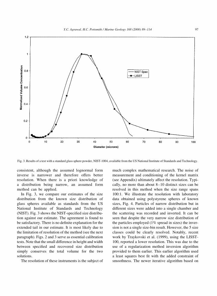
In Fig. 3, we compare our estimates of the size

distribution from the known size distribution of

glass spheres available as standards from the US

National Institute of Standards and Technology

(NIST). Fig. 3 shows the NIST-speci®ed size distribu-

tion against our estimate. The agreement is found to

be satisfactory. There is no de®nite explanation for the

extended tail in our estimate. It is most likely due to

the limitation of resolution of the method (see the next

paragraph). Figs. 2 and 3 serve as essential calibration

tests. Note that the small difference in height and width

between speci®ed and recovered size distribution

simply conserves the total volume for the two

solutions.

The resolution of these instruments is the subject of

much complex mathematical research. The noise of

measurement and conditioning of the kernel matrix

(see Appendix) ultimately affect the resolution. Typi-

cally, no more than about 8±10 distinct sizes can be

resolved in this method when the size range spans

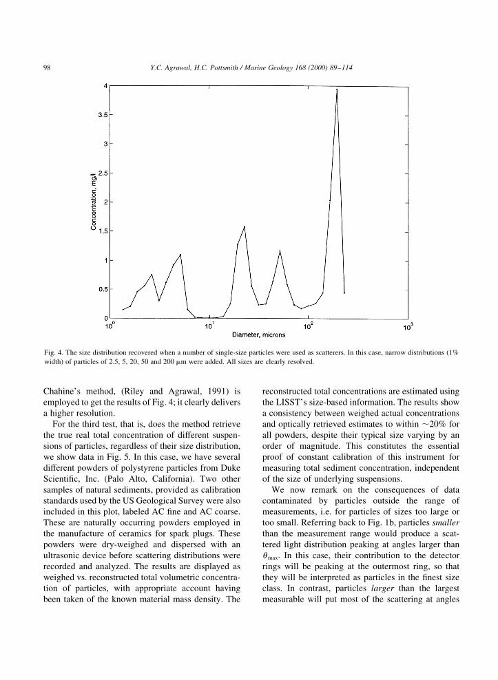
100:1. We illustrate the resolution with laboratory

data obtained using polystyrene spheres of known

sizes, Fig. 4. Particles of narrow distribution but in

different sizes were added into a single chamber and

the scattering was recorded and inverted. It can be

seen that despite the very narrow size distribution of

the particles employed (1% spread in sizes) the inver-

sion is not a single size-bin result. However, the 5 size

classes could be clearly resolved. Notably, recent

work by Traykovski et al. (1999), using the LISST-

100, reported a lower resolution. This was due to the

use of a regularization method inversion algorithm

provided to them earlier. This earlier algorithm used

a least squares best ®t with the added constraint of

smoothness. The newer iterative algorithm based on

Y.C. Agrawal, H.C. Pottsmith / Marine Geology 168 (2000) 89±114 97

Fig. 3. Results of a test with a standard glass sphere powder, NIST-1004, available from the US National Institute of Standards and Technology.

Chahine's method, (Riley and Agrawal, 1991) is

employed to get the results of Fig. 4; it clearly delivers

a higher resolution.

For the third test, that is, does the method retrieve

the true real total concentration of different suspen-

sions of particles, regardless of their size distribution,

we show data in Fig. 5. In this case, we have several

different powders of polystyrene particles from Duke

Scienti®c, Inc. (Palo Alto, California). Two other

samples of natural sediments, provided as calibration

standards used by the US Geological Survey were also

included in this plot, labeled AC ®ne and AC coarse.

These are naturally occurring powders employed in

the manufacture of ceramics for spark plugs. These

powders were dry-weighed and dispersed with an

ultrasonic device before scattering distributions were

recorded and analyzed. The results are displayed as

weighed vs. reconstructed total volumetric concentra-

tion of particles, with appropriate account having

been taken of the known material mass density. The

reconstructed total concentrations are estimated using

the LISST's size-based information. The results show

a consistency between weighed actual concentrations

and optically retrieved estimates to within ,20% for

all powders, despite their typical size varying by an

order of magnitude. This constitutes the essential

proof of constant calibration of this instrument for

measuring total sediment concentration, independent

of the size of underlying suspensions.

We now remark on the consequences of data

contaminated by particles outside the range of

measurements, i.e. for particles of sizes too large or

too small. Referring back to Fig. 1b, particles smaller

than the measurement range would produce a scat-

tered light distribution peaking at angles larger than

umax. In this case, their contribution to the detector

rings will be peaking at the outermost ring, so that

they will be interpreted as particles in the ®nest size

class. In contrast, particles larger than the largest

measurable will put most of the scattering at angles

Y.C. Agrawal, H.C. Pottsmith / Marine Geology 168 (2000) 89±11498

Fig. 4. The size distribution recovered when a number of single-size particles were used as scatterers. In this case, narrow distributions (1%

width) of particles of 2.5, 5, 20, 50 and 200 mm were added. All sizes are clearly resolved.

smaller than umin. A `leakage' will now result primar-

ily at the smallest, inner rings, thus these particles will

be interpreted as additional large particles. It might

thus be expected that whenever particles outside the

measurable range are present, their scattered power

would leak into the nearest size particles that are

within the range of measurement. However, in these

cases, the method fails to maintain correct calibration

for total suspended concentration.

3.4. Small scale turbulence and small number

statistics at large particle sizes

The theory of turbulence predicts that passively

advected scalars (e.g. particle concentration) exhibit

small scale structure similar to ¯uid motions. In other

words, variability of Cn can be expected at scales

down to micro-scales. The laser beam in Fig. 1a

crosses several such structures, effectively integrating

the concentration along a line of ®nite thickness. Thus,

the observed particle concentration will exhibit noise-

like random variations caused by the small-scale

structure within the laser beam. Furthermore, just as

velocity averaging times must take into account the

integral time scales for velocity (given by z=U), so also

to obtain true mean concentration of particles, aver-

aging of concentration over several integral time

scales is necessary.

An unfortunate consequence of the relatively small

sample-volume dimensions of the laser diffraction

instruments (typical volume is 2 cm3) is that when

the number density of particles is small, as is typical

Y.C. Agrawal, H.C. Pottsmith / Marine Geology 168 (2000) 89±114 99

Fig. 5. The relationship between known and measured total concentration of suspended particles for several different powders. A single linear

®t indicates the independence of calibration from size-distribution. At high concentrations, departure from the 1:1 line arises when beam

transmission drops below about 30%, i.e. as multiple-scattering effects become increasingly signi®cant.

Y.C. Agrawal, H.C. Pottsmith / Marine Geology 168 (2000) 89±114100

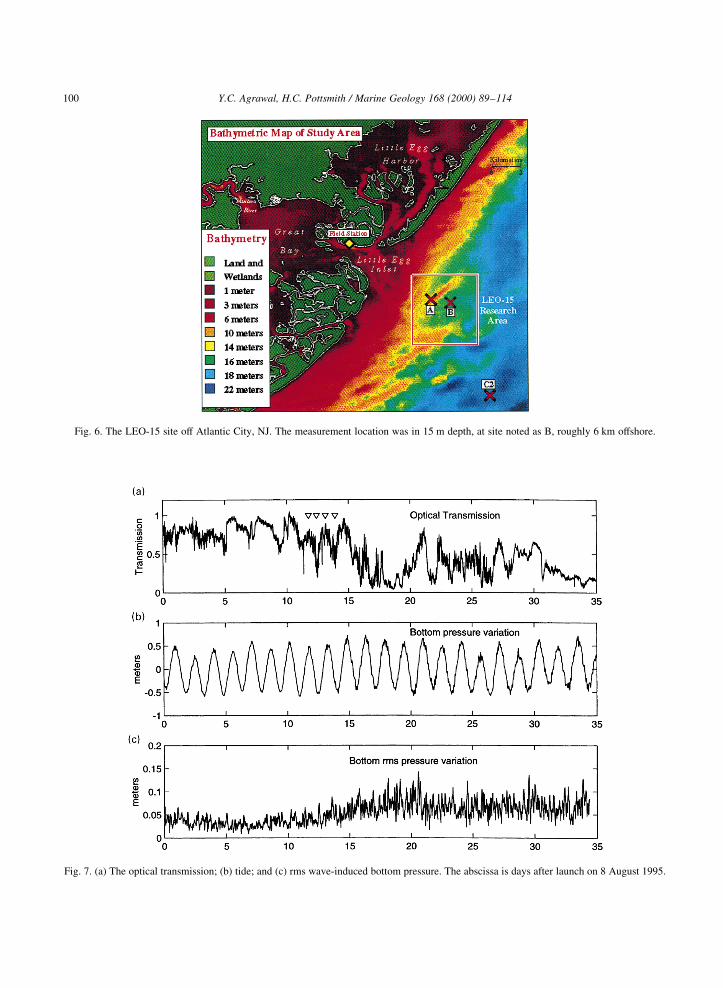
Fig. 6. The LEO-15 site off Atlantic City, NJ. The measurement location was in 15 m depth, at site noted as B, roughly 6 km offshore.

Fig. 7. (a) The optical transmission; (b) tide; and (c) rms wave-induced bottom pressure. The abscissa is days after launch on 8 August 1995.

for the largest particles (e.g. ¯ocs or marine

aggregates), statistical variability of the particle

number in the sample volume itself becomes large.

In interpreting ®eld data, it is important to bear this

in mind. Of course, averaging over several scans, in

effect, increases the sample volume size and thereby

reduces this variability.

3.5. Field tests

We illustrate data from a ®eld experiment carried

out on the New Jersey coast at the LEO-15 Observa-

tory maintained by the National Undersea Research

Program. The program is funded by the US National

Oceanic and Atmospheric Administration (NOAA).

Fig. 6 shows the location of the experiment, which

is roughly 4 miles offshore, east±northeast of Atlantic

City, New Jersey. The water depth is 15 m and the

topography is a dynamic ®eld of sand ripples. In this

bottom boundary layer experiment, a suite of instru-

ments was placed to record currents, bottom topogra-

phy, and suspended sediment concentration and size

distributions. The data that we have selected will illus-

trate the point that the size distribution responds to

local forcing through resuspension, so that as the

forcing weakens, so does the concentration of the

larger size classes.

Two LISST-100 instruments were placed on a

single tripod in this experiment at the LEO-15 site.

The two instruments were placed at heights-above-

bed of 0.3 and 1.5 m. The optical transmission and

pressure measured by the auxiliary sensors on the

LISST (showing tides) during the experiment are

shown in the top two panels of Fig. 7. On the bottom

panel, we show the pressure variance as an indication

of surface wave activity. The pressure signal on the

Y.C. Agrawal, H.C. Pottsmith / Marine Geology 168 (2000) 89±114 101

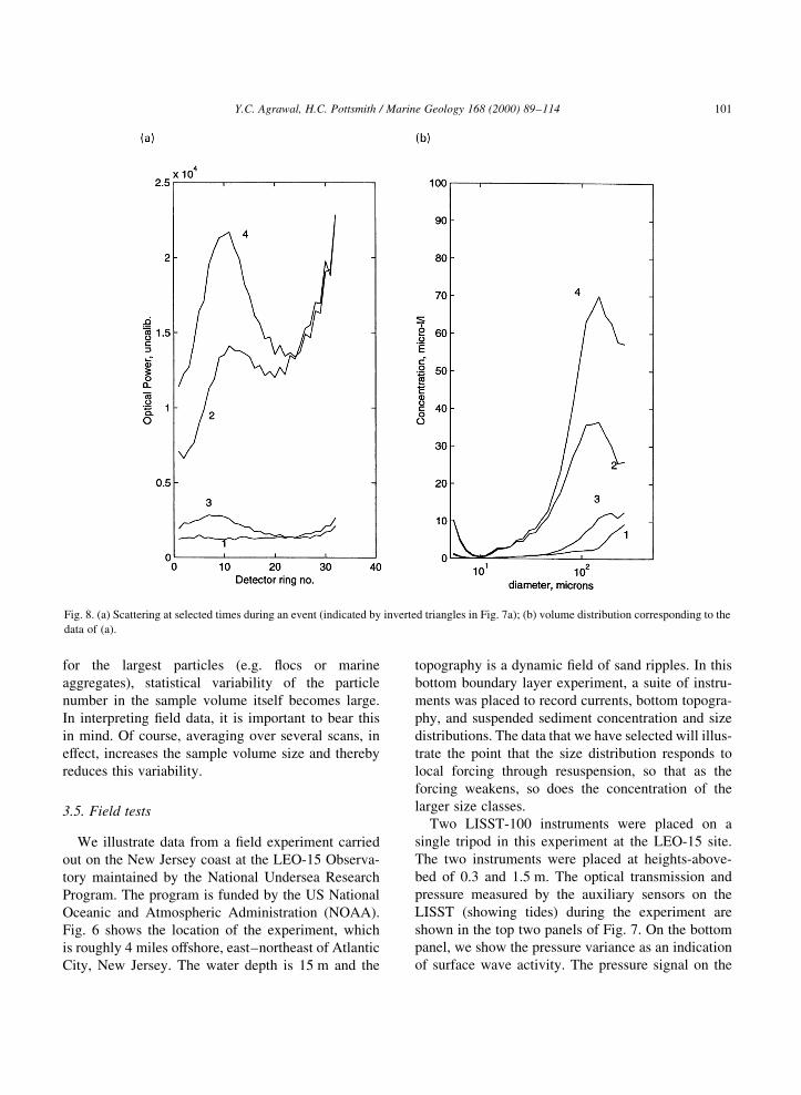
Fig. 8. (a) Scattering at selected times during an event (indicated by inverted triangles in Fig. 7a); (b) volume distribution corresponding to the

data of (a).

bottom related to gravity waves is computed as

follows. As pressure was sampled at 15 min intervals,

tides and surface waves are separated by ®rst high-

pass ®ltering the pressure record. This provides

samples of wave-height at the 15 min intervals.

These realizations of wave-height are then squared

and convolved with an 8-point top-hat ®lter to gener-

ate smooth estimates of mean-square wave-height

during the course of the experiment. The arrows on

this optical transmission record indicate the duration

from which scattering distribution records are

analyzed. It is seen that when the optical transmission

is higher (clearer water, curves 1&3 in 8a), the

maxima of the scattering curves occur at the inner-

most rings even though there is relatively less scat-

tered light. This corresponds to large particles in the

size distribution (curves 1&3, 8b). At the valleys in

the transmission curve (Fig. 7, top panel, second and

fourth inverted triangles), a lot more scattered light is

seen but with a peak at somewhat larger angles. This

implies smaller particles (curves 2&4, Fig. 8a and b).

The data suggest that during weaker forcing, when

large, dense primary particles can not be supported

by turbulence, ¯ocs must form with the characteristic

strong scattering at the smaller angles. These might

break up with stronger forcing, when also, an addi-

tional supply of sediment is made available to the

water column. We have observed similar patterns in

the Coastal Mixing and Optics experiment (Agrawal

and Traykovski, 2000).

Theory has predicted, as described in the introduc-

tory sections of this paper, that vertical gradients in

concentration can be expected for particles whose

settling velocities approach kup. Such observations

are possible with two vertically placed instruments.

The use of vertical gradients in size distribution

using the (Rouse, 1937; #1255) formulation suggests

possibilities of inferring the particle settling veloci-

ties. We shall examine the data from this standpoint

in a future publication.

4. LISST-ST

This instrument for measurement of the size-depen-

dent settling velocity distribution without assumption

of particle density is similar to the LISST-100. The

optics end of the instrument is enclosed in a settling

tube of 30 cm length. The settling column, Fig. 9,

which is enclosed in this 5 cm diameter settling

tube, consists of a 5 cm £ 1 cm wide £ 30 cm tall

rectangular volume. The rectangular column reduces

¯ow Reynolds number signi®cantly from the round

tube for the draw-in velocities. This feature is incor-

porated to assure faster suppression of turbulence in

order to obtain good estimates of the rapidly falling

larger particles. The settling tube has openings at the

top and bottom. Two motors are incorporated in the

system. One motor operates the doors and the second

powers a propeller in the settling tube, placed just

Y.C. Agrawal, H.C. Pottsmith / Marine Geology 168 (2000) 89±114102

Fig. 9. The settling column, along with the propeller and sliding

doors. Top and bottom lids are not shown. The column is 5 cm in

diameter, and 30 cm tall from the inlet to the laser beam.

below the laser beam. Vertically sliding doors with

radial `O'-ring seals are used to open and close the

doors. The cycle of operation is as follows: before

closing the doors, the motorized propeller in the

settling tube is powered up. Its function is to draw

in a new sample. The sample enters the settling tube

at the top, and is blown out at the bottom. A short-time

(4 s.) is allowed to elapse after the propeller power is

turned off. This ensures ®lling the tube with new ¯uid,

unaffected by propeller motion. At this time, the doors

are rapidly closed, in about 50 m s. This begins the

settling experiment. Data are taken at logarithmically

scheduled sampling intervals. In all, 83 scans are

saved over a day. At the end of the settling experi-

ment, the propeller is powered so that its vigorous

turbulence cleans the settling column and the optics

windows. The doors are opened, so that the propeller

blows the stirred water out, and at the same time

draws in a new sample. This begins the next cycle

of data acquisition.

Consider now the evolution of size distribution at

the optics block in the lower part of the settling

column where the laser senses size distribution. In

the case of a homogeneous suspension, i.e. all parti-

cles having the same mass density, each particle size

class will traverse the 30 cm settling tube at its own

unique settling velocity, determined solely by

diameter. Assuming that the settling column was ®lled

with a well-mixed sample of water, the concentration

history of any single size class of particles can be

expected as follows. As particles of this size class

settle, at some point in time, those particles that

were at the top of the settling column reach the laser

beam. Until this time, the concentration observed at

the laser beam can be expected to be constant, equal to

the ®ll-up concentration. Any apparent variations in

concentration prior to this time can arise due to imper-

fect mixing and small number statistics of the parti-

cles. Further settling causes the particles to fall

through the 6-mm diameter laser beam leaving no

more particles of this size to produce laser scattering.

Thus, over a duration corresponding to the time to fall

through the laser beam, the concentration for any size

class of particles will go from its natural value at ®ll-

up, to zero. Thus, both the onset of the decline in the

idealized constant concentration history, and the

length of duration of the sloping region will be

uniquely related to a particular particle size. This is

the idealized expectation. In reality, a few effects

complicate observations. First, natural particles are

seldom of a homogeneous composition, so that a

variation in particle density will cause a smearing of

the concentration pro®le. Second, the existence of

residual turbulence from the ®ll-in period smears the

measurement of settling velocity for the largest parti-

cles. A third factor is particularly frustrating, but only

in the laboratory: convection currents caused by

temperature changes with the cycling of ventilation

systems. It is worth noting that turbulence or convec-

tive motions must be weaker than the smallest settling

velocity of interest, in order to make a correct

measurement. Such conditions are dif®cult to achieve

in the laboratory for the smallest particles, whose

settling velocities may be a small fraction of a mm/

s, in effect setting the limit of measurable small-parti-

cle settling-velocity. The requirement that turbulence

or convection be much weaker than the smallest

settling velocity of interest is fundamental, not

speci®c to any technique. The thin settling column

of the LISST-ST is a couple of orders of magni-

tude thinner than typical other settling tubes, e.g.

the ROST device (roughly 30 cm £ 20 cm cross-

section) employed by Hill et al. (1994), or the

INSSEV of Fennessy et al. (1994). The data we

show below indicate that, signi®cantly, turbulence

in our settling column is indeed fully suppressed

so that not only does the water clarity increase

monotonically, but also the smallest measurable

particles do settle out over a time that is reason-

ably predicted by Stokes law.

In order for the settling histories to be employed for

estimation of settling velocity, it is necessary that the

concentration measurements for each size class be

totally independent of any other. Smoothing, as

often employed in least squares inverse algorithms,

works against statistical independence. Thus, one

must ®rst ask the question: how many truly indepen-

dent size classes are derivable from the multi-angle

scattering data. In a landmark paper, Hirleman (1987)

showed that the answer depends on the conditioning

of the forward matrix. Typically, with a 100:1 range

of scattering angles, only about eight truly indepen-

dent size classes can be obtained. Each of these size

classes contains particles spanning a size range

1.78:1. We offer this summary view for quick

reference; the interested reader may understand the

Y.C. Agrawal, H.C. Pottsmith / Marine Geology 168 (2000) 89±114 103

relationship between measurement noise and the

information content of the data by referring to Hirle-

man (1987).

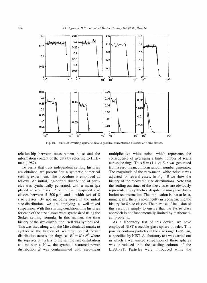
To verify that truly independent settling histories

are obtained, we present ®rst a synthetic numerical

settling experiment. The procedure is employed as

follows. An initial, log-normal distribution of parti-

cles was synthetically generated, with a mean (m)

placed at size class 12 out of 32 log-spaced size

classes between 5±500 mm, and a width (s ) of 8

size classes. By not including noise in the initial

size-distribution, we are implying a well-mixed

suspension. With this starting condition, time histories

for each of the size classes were synthesized using the

Stokes settling formula. In this manner, the time

history of the size-distribution itself was synthesized.

This was used along with the Mie calculated matrix to

synthesize the history of scattered optical power

distribution across the rings, as �E i � �K p �Ni where

the superscript i refers to the sample size distribution

at time step i. Now, the synthetic scattered power

distribution �E was contaminated with zero-mean

multiplicative white noise, which represents the

consequence of averaging a ®nite number of scans

across the rings. Thus �E � �1 1 e� �E: e was generated

from a zero-mean, uniform random number generator.

The magnitude of the zero-mean, white noise e was

adjusted for several cases. In Fig. 10 we show the

history of the recovered size distributions. Note that

the settling out times of the size classes are obviously

represented by synthetics, despite the noisy size distri-

bution reconstruction. The implication is that at least,

numerically, there is no dif®culty in reconstructing the

history for 8 size classes. The purpose of inclusion of

this result is simply to ensure that the 8-size class

approach is not fundamentally limited by mathemati-

cal problems.

As a laboratory test of this device, we have

employed NIST traceable glass sphere powder. This

powder contains particles in the size range 1±85 mm,

as speci®ed by NIST. A laboratory test was carried out

in which a well-mixed suspension of these spheres

was introduced into the settling column of the

LISST-ST. Particles were introduced while the

Y.C. Agrawal, H.C. Pottsmith / Marine Geology 168 (2000) 89±114104

Fig. 10. Results of inverting synthetic data to produce concentration histories of 8 size classes.

Y.C. Agrawal, H.C. Pottsmith / Marine Geology 168 (2000) 89±114 105

Fig. 11. History of: (a) optical transmission; and (b) scattering distribution during the settling experiment using glass spheres.

Fig. 12. Concentration history of 8 size classes for the NIST standard glass spheres. The solid lines show the estimates of concentration, the dots

indicate error of the estimate. When error exceeds the estimates, the size class history is fully discarded.

instrument was submerged in an approximately

constant temperature tank. Scattered optical power

distribution on the detector rings was recorded on a

logarithmic time schedule, with samples acquired a

few seconds apart initially, and several thousand

seconds apart toward the end. The settling experiment

lasted a full 24-hour duration. During this time, 83

scans were stored. As usual, the scattering signature

of the suspension at any of the 83 scans was calculated

by subtracting the zscat from the recorded data. The

optical transmission and scattered optical power

history are shown, respectively, in Fig. 11a and b.

The water monotonically gets clearer as particles

settle. Similarly, the scattering signature during the

course of settling shows a shift in the location of the

peak to the right, i.e. to the larger rings, as would be

expected with reduction in large particles that scatter

into small angles. These data are inverted using an 8-

size class inverse. Fig. 12 shows the settling history.

In this case, note ®rst that the ®rst size class (5±8 mm)

is empty as very little mass was present in the powder.

The size classes 3±5 contain the bulk of the particles,

and these are displayed in c±e. The dots on each plot

show the error of the estimate, computed from the

inverse of the data and the ®t. Thus, when the noise

level represented by the dots is small compared to the

signal level, settling velocity estimates from these

data can be trusted. This criterion serves as a guide

for interpreting the settling velocity estimates. It

follows that again, there is negligible mass in the

larger size classes, as is evidenced by large noise

spikes in f±h.

The settling history of each size class is converted

to a settling velocity following an optimization proce-

dure. Assuming homogeneity within a size class, the

problem of estimating the settling velocity becomes a

one-parameter optimization problem. Consider the

settling time for particles in size class n. This size

class contains particles of sizes aminrn21 to aminr

n:

Now, a single idealized concentration is constructed

that has a constant concentration for the duration

30 cm=wf;n; followed by a linearly sloping concentra-

tion as the particles fall through the laser beam, and a

zero concentration thereafter. The sloping section has

a duration such that, the smallest to the largest parti-

cles in the size class fall through the 6mm beam in this

Y.C. Agrawal, H.C. Pottsmith / Marine Geology 168 (2000) 89±114106

Fig. 13. Estimates of settling velocity of glass spheres, compared with Stokes settling. Note that as the size distribution is quite narrow (Fig. 3,

and also Fig. 12), several size classes are unpopulated. This produces noisy estimates for the nearly empty size bins. As a result, the settling

velocity can be estimated for only size classes 2±5.

Y.C. Agrawal, H.C. Pottsmith / Marine Geology 168 (2000) 89±114 107

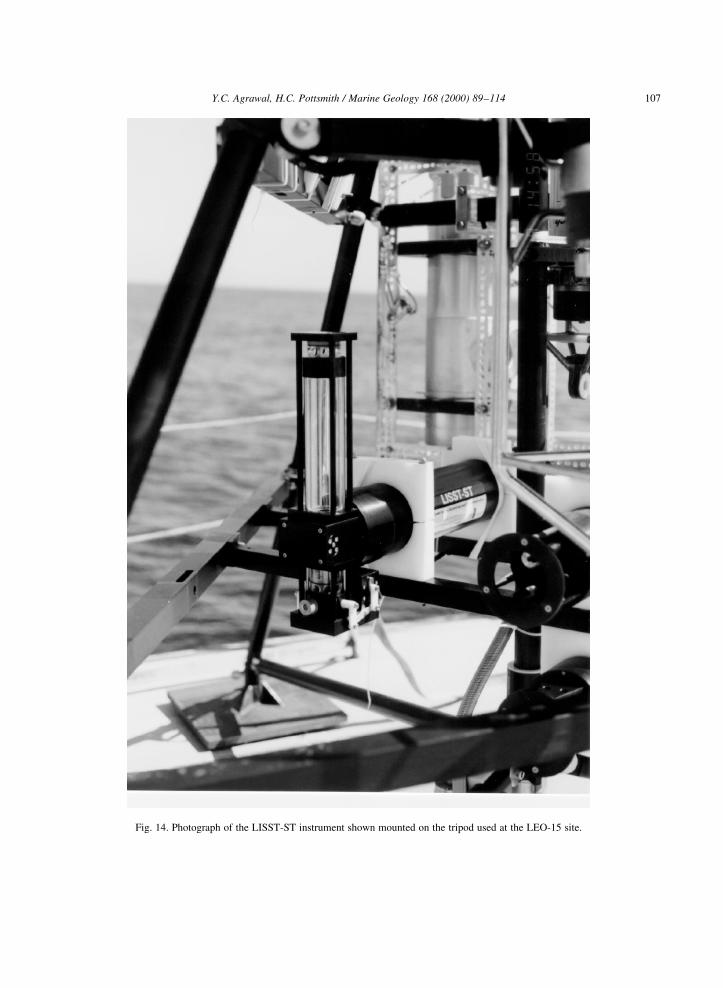
Fig. 14. Photograph of the LISST-ST instrument shown mounted on the tripod used at the LEO-15 site.

time. This duration begins at 30=wf;;n: The smallest

particles in the size class fall through the laser beam

over a time equal to 6 mm=wf;n21 whereas the largest

particles within the size class fall through over a time

equal to 6 mm=wf;n: Thus the length of the sloping part

of concentration history is expected to be

6=�1=wf;n21 2 1=wf;n�: In effect, the square parentheses

arise due to the ®nite size-width of size class n. Now

since r � 1:78 and settling velocity can be reasonably

expected to follow Stokes' law, the settling velocities

will vary within a size class by r2 � 3:2: Thus, the

break in the sloping duration will begin at some time

TB and end at 3.2 TB. The difference, 2.2 TB is the

length of the sloping region.

One now ®nds a TB which minimizes the mean-

square difference between the idealized and normal-

ized history of any size class. Mathematically, this is

expressed as follows. Let the time history of concen-

tration in size class n be called Cn(t), then one de®nes

an idealized history by the function F (t) such that it is

constant for time TB equal to 30 cm=wf;n21; gradually

decreases to zero over the time it takes particles of

sizes in the size-class to fall through 6 mm, i.e. 2.2 TB

and is zero thereafter:

F�t� � 1=TB

ZT

0Cn�t� dt for 0 , t , TB;

� F�TB�2 �t 2 TB�=2:2TB for TB , t , 3:2TB;

� 0 for t .� TB

�9�The best estimate of settling time TB is found by mini-

mizing the least square difference of the history with

the idealized history F�t�; i.e.:

d=dTB{�Cn�t�2 F�t�� 2} � 0; �10�The procedure is implemented numerically. The solu-

tions TB for each size class are used separately to

estimate the settling velocity for that size class.

These data are shown in Fig. 13. It can be seen that

the experimental data match Stokes settling to an error

of nearly 20%. We are not certain as to the cause of

Y.C. Agrawal, H.C. Pottsmith / Marine Geology 168 (2000) 89±114108

Fig. 15. The optical transmission for 10 successive days.

the apparently small bias, but we speculate that the

bias results from the observed longer than theoretical

sloping region of the concentration history, which in

turn, probably is caused by convective currents in the

laboratory excited by ventilation.

A ®nal comment regarding estimation of settling

velocities with a sampling system concerns ¯oc

break-up. Gibbs and associates have published a

series of articles on ¯oc break-up (Gibbs, 1982;

Gibbs and Konwar, 1982, 1983). These articles

concern themselves with breakage of ¯ocs in the

course of, respectively, analysis with a particular opti-

cal blockage instrument, due to pipetting, and during

Niskin bottle sampling. We have not been able to

quantify such effects in this study. A noteworthy

detail is that the sample water is drawn through

12.7 mm holes at the top of the settling column.

4.1. Field tests

The ®eld settling velocity data presented in this

paper were obtained in the NURP program already

mentioned in an earlier section, although the current

data were acquired in a deployment at the site in

December 1997. The LISST-ST was mounted on a

tripod and deployed at the approximately 15 m

depth for bottom boundary layer measurements from

a tripod. The instrument is displayed on the tripod in

Fig. 14. A settling experiment was begun each

midnight and lasted most of the 86,400 remaining

seconds of the day. Upon examination of data, the

settling tube appears to have operated routinely for

the ®rst 21 days of the deployment.

We display two key sets of data, again with the

instrumentation point of view, leaving detailed scien-

ti®c discussion to a later publication. The ®rst is a

history of optical transmission on 10 successive

experimental days. In this case (Fig. 15) although

due to different environmental conditions on different

days, the initial optical transmission varies, the optical

transmission increases in time, i.e. water monotoni-

cally clears as particles settle. Again, signi®cantly,

this observation is consistent with expectation, and,

it contrasts with the earlier settling tube work of Zane-

veld et al. (1982), and Hill et al. (1994). We interpret

this monotonic increase in optical transmission to

mean that there was no leakage into or out of the

settling tube and that the initial turbulence was

suppressed in a time-scale shorter than the shortest

time at which any signi®cant settling out occurs.

Y.C. Agrawal, H.C. Pottsmith / Marine Geology 168 (2000) 89±114 109

Fig. 16. Concentration history for the 8 size classes during one of the 10 experiments shown in Fig. 15.

Furthermore, the similarity of the transmission

histories suggests that the particles were of a similar

settling velocity distribution. This becomes evident

when it is seen that the optical attenuation t is propor-

tional to the sum of the concentration of the various

component size classes. As each size class settles out,

the transmission would then show an increase. Thus, a

similar slope in the history on several days implies

settling out of particles at near-equal times.

The concentration histories derived from the scat-

tering are displayed in Fig. 16. The 8 size classes are

identical for those of Fig. 11. In this case, we see a

settling rate that is slower than the Stokes settling rate

for siliceous particles in the smallest size classes, and

an even greater divergence for the largest size classes.

The fact that the particles in the smallest size classes

settle out at all indicates that thermally driven

residual motions are smaller than the smallest measur-

able settling velocity: 30 cm=8:6 £ 104 s; or 3:5 £1024 cm=s: In a separate paper, we shall publish the

details of consistency between settling rate estimates

obtained on different days. For now we note that the

validity of Stokes settling for the lower Reynolds

numbers, as veri®ed in Fig. 11, permits us to estimate

the density of particles from their measured settling

velocities. In Fig. 17, the settling velocity distribution

is displayed for the particles at the LEO-15 site. Also

displayed is a slope-2 line that would correspond to

constant density particles falling in Stokes regime.

The fact that the marine particles deviate from this

behavior is an indication of the existence of ¯ocs.

The departure from constant density line is more

exaggerated at the larger sizes, suggesting that the

larger particles are loose aggregates.

A simple ®t to the data of Fig. 17 suggests a size vs.

settling velocity relationship as:

wf�d� � 0:45 £ 1023a1:17 �11�The generalized validity of this relation will be

explored from the data at LEO-15 in a subsequent

paper.

5. Discussion

The measurement of particle size distributions is of

intrinsic interest to the marine scientist, whether from

the point of view of sediment transport, biological

Y.C. Agrawal, H.C. Pottsmith / Marine Geology 168 (2000) 89±114110

Fig. 17. Settling velocity estimates from a set of settling experiments at LEO-15.

process studies or even bubble formation. The devel-

opment of capabilities to estimate total suspended

sediment concentration correctly, without errors intro-

duced by changes in the natural particle size distribu-

tion is sure to add to the researchers' and the

engineers' bag of tools. The autonomous capability

of these devices permits long-term use for observa-

tions of episodic events, which in some places, do

most of the transport of sediments.

The instrumentation described here does have

limitations. For example, the consequence of the

presence of very light aggregate type particles to

the determination of size distribution is not known.

The small-angle scattering properties of these marine

aggregates need to be studied. Also, there is a strong

body of literature suggesting, from photographs, that

stringy scatterers are present in aquatic environments,

(e.g. Honjo et al., 1984). Here, the sphere approxima-

tion is, of course, unsuitable. Diffraction theory

predicts that thin cylinders produce streaked scatter-

ing in a plane normal to the plane containing the

cylinder. Thus, strings produce streaks across the

face of the ring-detector. If a streak lies on one quad-

rant of the detector, it produces a bias in that quadrant.

This is frequently recognizable in the data as a

sawtooth shape in the scattering signature. The same

behavior has also been observed in the laboratory

when scattering is observed from natural particles in

still water. When turbulence is introduced, the scatter-

ing signature becomes smooth instantly. This effect is

due to the establishment of preferred orientation of

particles falling in still water. As these particles are

also not spherical, the scattering has preferred orien-

tations, again producing a sawtooth signature in the

scattering data. These characteristics are helpful hints

in learning more about the nature of the scatterers,

although the quanti®cation of such interpretation is

as yet not possible.

A second limitation is in the range of turbidity that

can be measured. We have observed that when the

optical transmission is less than 30%, multiple-scat-

tering effects begin to appear. This refers to the re-

scattering of scattered light. The lower the transmis-

sion, the stronger the effects of multiple scattering.

Theoretical investigations of multiple scattering

reveal that if such effects are ignored, the recovered

particle size distribution shows a bias toward the small

sizes. Algorithms for multiple scattering are available

in the literature as applied to this problem (Hirleman,

1991).

When measuring settling velocities, there is a

continual concern regarding the breakup of fragile

aggregates in the process of drawing of a sample.

There is no known way of estimating such ¯oc

damage at present. Perhaps an in-situ photographic

approach can be used for an assessment.

Acknowledgements

This paper is the result of several years of work

supported ®rst by Dr Joseph Kravitz of the Of®ce of

Naval Research under current contract no. N00014-

95-C-0101, by Dr Curtis Olsen of the Department of

Energy, contract no. DE-FG03-96-ER62179 and via a

grant from NOAA under the NURP program managed

by Dr Waldo Wake®eld at Rutgers University. The

authors acknowledge the many constructive

comments of the reviewers who acquainted us with

the work of Gibbs cited in the bibliography.

Appendix A

The size distribution function n(a) is de®ned so that

n�a�da represents the number of particles per unit

volume of water, of size a in a size range da. Thus

the area distribution is a2n�a� and the volume distri-

bution is given by a3n�a�: We treat the measurement

of optical attenuation, background scattering, both of

which are necessary auxiliary measurements, and

inversions below.

A.1. Optical attenuation

With reference to Fig. 1, let the laser output power

be Pl. A fraction of this power �1 2 a�Pl is split off

and sensed by the reference detector, Pr. The remain-

ing, aPl enters water after some losses due to scatter-

ing off surfaces in the prism and pressure-resistant

window. If h trans is the overall optical ef®ciency of

the components from the beam splitter till the laser

beam enters water, then the laser power entering water

will be � ah transPl. For the sake of simplicity, de®ne

P0 � ahtransPl: Consider ®rst the case of pure ®ltered

water. The power reaching the receiving window will

be attenuated due to absorption in water. It is conven-

Y.C. Agrawal, H.C. Pottsmith / Marine Geology 168 (2000) 89±114 111

tional in ocean optics literature to use the symbol a for

pure water absorption (in m21) so that the laser power

reaching the receiving window will be e2alP0: Further

optical losses due to re¯ections off optical surfaces

can be included as another optical ef®ciency factor,

h recv so that the power sensed by the `transmiss-

ometer' photodiode is e2alP0hopt2: Combining the

factors ah trans h recv into an overall optical ef®ciency

hopt � ahtranshrecv; one sees that for the case of pure

water, the `transmissometer' diode sees a laser power

given by

Pt;clear � e2alhoptPl

�A1�The introduction of absorptive and/or scattering mate-

rial, with an additional attenuation of light by absorp-

tion and scattering represented by cA (m21), will

clearly change the power incident on the transmiss-

ometer photodiode to

Pt;turbid � exp{ 2 �a 1 cA�l}hoptPl. �A2�From the ratio of Eqs. A2 and A1, the transmissometer

photodiode measures the additional cA due to the

dissolved and suspended material. When there is no

dissolved absorbing material and the particles are

non-absorbing, cA � b; the total scattering, so that a

direct measure of total scattering by particles is

obtainable. In general, the measured attenuation will

be the sum of that due to absorption and scattering by

particles and due to any dissolved absorptive material.

These quantities are of interest to optical oceanogra-

phers concerned with light propagation studies.

A.2. Background light

The measurement of background light and its

adequate subtraction from the total signal at the ring

detector is important, especially when the scattering

from particles is weak. Buchele (1988) has shown that

if the background light is measured in the absence of

scattering particles, then this background ®eld should

be ®rst multiplied by exp�2cAl� before subtracting

from the measurement which is the combined signal

from particles and optical surfaces. This is incorpo-

rated in Eq. (5).

A.3. Scattered light signal and inversion

For the geometry of Fig. 1, the optical power

scattered into a solid angle dV from a single particle

placed in the laser beam, at a distance x from the

transmitting window is given by:

I � �P0 e2cx=A��i1 1 i2� e2c�l2x� dV=k 2 �A3�

Where, i1 1 i2 are intensity functions de®ned in Van

deHulst (1957) (p. 129), and where we explicitly show

attenuation of the beam up to the particle as e2cx and

from the particle to the receiving window as e2c(l2x). It

follows that an elementary volume, of diameter A and

length dl with a particle number density n(a)da per

unit volume would produce a scattering given by

I1 � P0 e2cl�i1 1 i2�dl n�a�da dV=k 2 �A4�In the above, the attenuation coef®cient c is the sum of

absorption by water, dissolved material, and particles,

and attenuation by scattering by particles:

c � aw 1 ad 1 b �A5�Now, the solid angle in the focal plane is:

d V � u d u �A6�so that, one writes for the power sensed by a single

ring, after integrating along the optical path in water

and after including the optical ef®ciency of the receiv-

ing optics:

Ei �ZZ

hrecvP0 e2cl�i1 1 i2�dl n�a�u da du=k2; �A7�

or

Ei � P0hrecvl e2cl=k2

Zn�a�a2da

Z�i1 1 i2�a22u du

This equation, in a manner similar to Hirleman

(1987), is rewritten in the discretized form:

or �E � �P0hrecvl e2cl=k2� �KNA �A8�

Each element of the kernel matrix KÅ is the inner inte-

gral, and each element of the vector �NA is the area in

the size range, as represented by the outer integral of

Eq. (A7). The integrations are carried out, in angles

and sizes, respectively, over ri21umin , u , riumin

and r j21amin , a , rjamin:

The photo-current from the corresponding ring is

converted to a voltage using an operational ampli®er

circuit, and the voltage is digitized. If R is the respon-

sivity of the photo-diodes, and the gain (current-to-

voltage) is G, then the voltage sensed will be GR �E:

Y.C. Agrawal, H.C. Pottsmith / Marine Geology 168 (2000) 89±114112

With a 12-bit 5 V full-scale A/D converter, the digital

counts for the 32 rings will be given by the array dÅ:

�d � �4096=5�GR�P0hrecvl e2cl=k2� �K �NA �A9�

This is the array noted in Eq. (5). The laser power P0 is

simply a constant times the reference power Pr, the

power sensed by the reference sensor (see Fig. 1). We

now combine all the constants in front of the matrix

product to write:

�d � K�Pr e2cl� �K �NA or �d � KtPr�K �NA �A10�

The measured digital counts include the scattering

from background optical surfaces also, which is atte-

nuated by t exactly as scattering is. Thus the

measured digital counts are:

�d � KtPr� �K �NA 1 zscat� �A11�This is the basis for the formulation of Eq. (5). The

constant K can be computed from above, or it can be

estimated by calibrating a known particle size distri-

bution as in Eq. (7).

A.4. Solution for NÅ A

The inversion of Eq. (A3) is carried out using a

modi®ed Chahine method described by Riley and

Agrawal (1991). This is a non-linear iterative solution

and has been empirically determined to be the best

performer. According to this method, the �n 1 1�thiterate is computed from the nth by

Nn11A;i � Nn

A;i´j �A12�where j is the ratio of the measured scattering at the

ring corresponding to size i and the magnitude of the

predicted scattering at this ring from the previous iter-

ate. Once a reasonable convergence is reached, the

volume distribution is computed as (leaving out

factors of p):

VA;i � 4=3aiNA;i �A13�We have expressed this entire procedure in the short-

hand INV(S) in Eq. (7). It should be noted that the

mathematical problem of inversion continues to

receive attention of researchers. A recent survey

appears in a special issue of the journal Applied Optics

(vol. 30, no. 33, 1991). The interested reader is

encouraged to study the works of Twomey (1977)

and Hirleman (1987) which address the fundamental

information content of data in inverse problems.

References

Agrawal, Y.C., Pottsmith, H.C., 1993. Optimizing the kernel for

laser diffraction particle sizing. Appl. Opt. 32 (22), 4285±4286.

Agrawal, Y.C., Pottsmith, H.C., 1994. Laser diffraction particle

sizing in STRESS. Continental Shelf Res. 14 (10/11), 1101±

1121.

Agrawal, Y.C., Traykovski, P., 2000. Particles in the bottom bound-

ary layer: concentration and size dynamics through events. J.

Geophys. Res. (in press).

Bale, A.J., Morris, A.W., 1987. In situ measurement of particle

size in estuarine waters. Estuarine Coastal Shelf Sci. 24,

253±263.

Born, M., Wolf, E., 1975. Principles of Optics, Pergamon, New

York, p. 808.

Buchele, D.R., 1988. Particle sizing by weighted measurements of

scattered light, NASA-TM-100968, NASS.

Crawford, P., Hay, A.E., 1993. Determining suspended sand size

and concentration from multi-frequency acoustic backscatter . J.

Acoustic Soc. Am. 94, 3312±3324.

Dietrich, W.E., 1982. Settling velocity of natural particles. Water

Resour. Res. 18 (6), 1615±1626.

Downing, J.P., Sternberg, R.W., Lister, C.R.B., 1981. New instru-

mentation for the investigation of sediment suspension

processes in the shallow marine environment. Mar. Geol. 42,

19±34.

Dyer, K.R., et al., 1996. A Comparison of in-situ techniques for

estuarine ¯oc settling velocity measurements. J. Sea Res. 36

(1/2), 15±29.

Eisma, D., et al., 1996. Intercomparison of in-situ suspended matter

(¯oc) size measurements. J. Sea Res. 36 (1/2), 3±14.

Fennessy, M.J., Dyer, K.R., Huntley, D.A., 1994. INSSEV: an

instrument to measure the size and settling velocity of ¯ocs

in-situ. Mar. Geol. 117, 107±117.

Gentien, P., Lunven, M., Lehaitre, M., Duvent, J.L., 1995. In-situ

depth pro®ling of particle sizes. Deep-Sea Res. 42 (8), 1297±

1312.

Gibbs, R.J., 1982. Floc breakage during HIAC light-blocking analy-

sis. Environ. Sci. Technol. 16 (5), 298±299.

Gibbs, R.J., Konwar, L.N., 1982. Effect of pipetting on mineral

¯ocs. Environ. Sci. Technol. 16 (2), 119±121.

Gibbs, R.J., Konwar, L.N., 1983. Sampling of mineral ¯ocs using

Niskin bottles. Environ. Sci. Technol. 17 (6), 374±375.

Hay, A.E., Sheng, J., 1992. Vertical pro®les of suspended sand

concentration and size from multifrequency acoustic backscat-

ter. J. Geophys. Res. 97 (C10), 15 661±15 677.

Hill, P.S., Sherwood, C.R., Sternberg, R.W., Nowell, A.R.M., 1994.

In situ measurements of particle settling velocity on the northern

California continental shelf. Continental Shelf Res. 14 (10/11),

1123±1138.

Hirleman, E.D., 1987. Optimal scaling of the inverse Fraunhofer

diffraction particle sizing problem: the linear system produced

by quadrature. Particle Characterization 4, 128±133.

Y.C. Agrawal, H.C. Pottsmith / Marine Geology 168 (2000) 89±114 113

Hirleman, E.D., 1991. General solution to the inverse near-forward-

scattering particle-sizing problem in multiple-scattering envir-

onments: theory. Appl. Opt. 30 (33), 4832±4838.

Honjo, S., Doherty, K.W., Agrawal, Y.C., Asper, V.L., 1984. Direct

optical assessment of large amorphous aggregates (marine

snow) in the deep ocean. Deep-Sea Res. 31 (1), 67±76.

Jones, S.E., Jago, C.F., 1996. Determination of settling velocity in

the Elbe estuary using quisset tubes. J. Sea Res. 36 (1/2), 63±67.

Lynch, J.F., Irish, J.D., Sherwood, C.R., Agrawal, Y.C., 1994.

Determining suspended sediment particle size information

from acoustical and optical backscatter measurements. Conti-

nental Shelf Res. 14 (10/11), 1139±1165.

Moody, J.A., Butman, B., Bothner, M.H., 1987. Near-bottom

suspended matter concentration on the continental shelf during

storms: estimates based on in-situ observations of light trans-

mission and a particle size dependent transmissometer claibra-

tion. Continental Shelf Res. 7 (6), 609±628.

Puls, W., Kuhl, H., 1996. Settling velocity determination using the

Bigdan settling tube and the Owen settling tube. J. Sea Res. 36

(1/2), 119±125.

Riley, J.B., Agrawal, Y.C., 1991. Sampling and inversion of data in

diffraction particle sizing. Appl. Opt. 30 (33), 4800±4817.

Rouse, H., 1937. Modern conceptions of the mechanics of ¯uid

turbulence. Trans. Am. Soc. Civil Engng 102, 463±554.

Smith, J.D., 1977. Modeling of Sediment Transport on Continental

Shelves, the Sea, Wiley, New York, pp. 539±577.

Swithenbank, J., Beer, J.m., Taylor, D.S., Abbot, D., McCreath,

G.C., 1976. A laser diagnostic technique for the measurement

of droplet and particle size distribution, AIAA, New York, pp.

76±79.

Thorne, P.D., Hardcastle, P., 1997. Acoustic measurements of

suspended sediments in turbulent currents and comparison

with in-situ sampling. J. Acoustic Soc. Am. 101, 2603±2614.

Traykovski, P., Latter, R., Irish, J.D., 1999. A laboratory evaluation

of the laser in-situ scattering and transmissometry instrument

using natural sediments. Mar. Geol. 159, 355±367.

Twomey, S., 1977. An Introduction to the Mathematics of Inver-

sion. Remote Sensing and Indirect Measurements, Elsevier,

Amsterdam, p. 243.

Van Leussen, W., 1996. The RWS ®eld settling tube. J. Sea Res. 36

(1/2), 83±86.

Van deHulst, H., 1957. Light Scattering by Small Particles, Dover,

New York, p. 470.

Wiberg, P.L., 1995. A theoretical investigation of boundary layer

¯ow and bottom shear stress for smooth, transitional, and rough

¯ow under waves. J. Geophys. Res. 100 (C11), 22 667±22 679.

Yariv, A., 1988. Optical Electronics, Holt, Rinehart, and Winston,

New York, p. 551.

Zaneveld, J.R.V., Sprinrad, R.W., Bartz, R., 1982. An optical

settling tube for the determination of particle size distribution.

Mar. Geol. 49, 357±376.

Y.C. Agrawal, H.C. Pottsmith / Marine Geology 168 (2000) 89±114114