This article was downloaded by: [194.27.18.18] On: 14 August 2014, At: 06:19Publisher: Institute for Operations Research and the Management Sciences (INFORMS)INFORMS is located in Maryland, USA
Operations Research
Publication details, including instructions for authors and subscription information:http://pubsonline.informs.org
Integrated Optimization of Procurement, Processing, andTrade of CommoditiesSripad K. Devalkar, Ravi Anupindi, Amitabh Sinha,
To cite this article:Sripad K. Devalkar, Ravi Anupindi, Amitabh Sinha, (2011) Integrated Optimization of Procurement, Processing, and Trade ofCommodities. Operations Research 59(6):1369-1381. http://dx.doi.org/10.1287/opre.1110.0959
Full terms and conditions of use: http://pubsonline.informs.org/page/terms-and-conditions
This article may be used only for the purposes of research, teaching, and/or private study. Commercial useor systematic downloading (by robots or other automatic processes) is prohibited without explicit Publisherapproval, unless otherwise noted. For more information, contact [email protected].
The Publisher does not warrant or guarantee the article’s accuracy, completeness, merchantability, fitnessfor a particular purpose, or non-infringement. Descriptions of, or references to, products or publications, orinclusion of an advertisement in this article, neither constitutes nor implies a guarantee, endorsement, orsupport of claims made of that product, publication, or service.
Please scroll down for article—it is on subsequent pages
INFORMS is the largest professional society in the world for professionals in the fields of operations research, managementscience, and analytics.For more information on INFORMS, its publications, membership, or meetings visit http://www.informs.org
We consider the integrated optimization problem of procurement, processing, and trade of commodities in a multiperiodsetting. Motivated by the operations of a prominent commodity processing firm, we model a firm that procures an inputcommodity and has processing capacity to convert the input into a processed commodity. The processed commodity is soldusing forward contracts, while the input itself can be traded at the end of the horizon. We solve this problem optimally andderive closed-form expressions for the marginal value of input and output inventory. We find that the optimal procurementand processing decisions are governed by price-dependent inventory thresholds. We use commodity markets data for thesoybean complex to conduct numerical studies and find that approximating the joint price processes of multiple outputcommodities using a single, composite output product and using the approximate price process to determine procurementand processing decisions is near optimal. Compared to a myopic spread-option-based heuristic, the optimization-baseddynamic programming policy provides significant benefits under conditions of tight processing capacities and high pricevolatilities. Finally, we propose an approximation procedure to compute heuristic policies and an upper bound to comparethe heuristic against, when commodity prices follow multifactor processes.
Area of review : Manufacturing, Service, and Supply Chain Operations.History : Received December 2008; revisions received August 2009, April 2010, November 2010, March 2011; accepted
April 2011.
1. IntroductionIn this paper we consider the problem of a firm that pro-cures an input commodity and earns revenues by processingand trading the processed product over a multiperiod hori-zon. The specific motivation for our study comes from theoperations of one of India’s largest private sector compa-nies, the ITC Group. In the year 2000, ITC embarked onthe e-Choupal initiative to deploy information and commu-nication technology (ICT) to reengineer the procurement ofcommodities from rural India. By purchasing directly fromthe farmers, and not just from the local spot markets, ITCsignificantly improved the efficiency of the channel and cre-ated value for both the farmer and itself. The initiative hasbeen hailed as an outstanding example of the use of ICTby a private enterprise to streamline supply chains, allevi-ate poverty, and bring about social transformation (Prahalad2005, Anupindi and Sivakumar 2007).
Managing the e-Choupal, or any other commod-ity processing operations, requires decisions regardingprocurement, processing, and trade of multiple commodi-ties. Consider soybean, one of the largest commodities pro-cured by ITC. Close to 70% of the soybean procured isprocessed at processing plants, while the rest is traded.
Beans are processed to produce soybean oil and soybeanmeal, both of which are traded through various channels.Because of uncertainty in both input and output commod-ity prices, it is important for processing firms to under-stand the relationship between procurement, processing,and trade decisions for multiple commodities and coordi-nate decisions across commodities and periods. Operationalconstraints such as procurement and processing capacitiesmake this task more complex. While different aspects of theproblem—procurement, processing, and trade—have beenstudied earlier, the integrated problem itself, even for oper-ations at a single node, has not received much attention inthe literature. In practice, firms consider the interdependen-cies between procurement, processing and trade decisions(see Plato 2001, for instance), but do so in a myopic fashionand ignore the dynamic nature of decisions.
In this paper we consider a multiperiod optimizationproblem in which a firm procures an input commodity,with the marginal cost of procurement equal to the spotprice of the commodity. The firm earns revenues by pro-cessing the input commodity and committing to sell theprocessed outputs using forward contracts in every period.In addition, the firm can also trade the input inventory withother processors at the end of the horizon. We model the
firm’s optimization problem as a stochastic dynamic pro-gram, with the procurement and processing decisions ineach period subject to capacity constraints. We provide aprecise, analytical description of the optimal policy struc-ture. We investigate the benefits of using a forward-lookingoptimization-based policy relative to myopic spread-option-based policies that are used in practice. We do this by con-ducting numerical studies using commodity markets datafor the soybean complex—soybean, soybean meal, and soy-bean oil. We summarize our results below.
1. We show that the optimal value function is separablein the input and output commodity inventories and is piece-wise linear and concave in the inventory levels. We deriverecursive expressions to quantify the marginal value of theinput and output commodity inventories.
2. We find that it is optimal for the firm to postpone theoutput trade against a forward contract with given maturityto the last possible period, i.e., the period just before thematurity of the forward contract; and the optimal outputcommitment policy is similar to the exercise of a compoundexchange option.
3. We characterize the optimal procurement and process-ing policy and find that the optimal decisions are governedby procure-up-to and process-down-to inventory thresholds,with these thresholds dependent on the realized prices andremaining horizon length.
4. Using commodity markets data for the soybean com-plex, we find that a myopic heuristic used in practice per-forms almost as well as the optimization-based dynamicprogramming policy under normal operating conditions.However, the dynamic programming policy provides sig-nificant benefits under conditions of tight processing capac-ities and high price volatilities.
5. The complexity in computing the dynamic program-ming policy increases rapidly as the number of outputproducts increases. We approximate multiple output com-modities as a single composite output to address thiscomputational complexity, and we find that this approxi-mation is near optimal.
The rest of the paper is organized as follows. In the nextsection, we review literature relevant to this research andposition our work. In §3, we solve the integrated procure-ment, processing, and trade decisions for a risk-neutral firmand obtain expressions for the marginal value of inventory.Section 3.1 presents the analysis for the case when a singleoutput commodity is produced upon processing the input,while §3.2 generalizes the result to a situation where multi-ple products are produced upon processing. Section 4 pro-vides numerical illustrations using commodity market datafor the soybean complex and describes the computation ofthe optimal policy when all commodity prices are driven bysingle factor mean reverting processes. The computationalpolicy described here can be extended to the case of multi-factor commodity process models using heuristics, whichbuilds on the works of Brown et al. (2010) and Lai et al.(2010). Details of the heuristic and computational results
are given in an appendix, provided as an online supple-ment to this paper. An electronic companion to this paper isavailable as part of the online version that can be found athttp://or.journal.informs.org/. Section 5 concludes the paperwith directions for future research.
2. Literature ReviewThe problem studied in this paper is related to the ware-house management problem originally studied by Bellman(1956) and Dreyfus (1957). The warehouse managementproblem deals with determining the optimal trading pol-icy for a commodity with constraints on the total inventorythat can be stored. Charnes et al. (1966) show that thevalue function is linear in the starting inventory level, andthey derive expressions for the marginal value of inventory.These papers do not consider constraints on the procure-ment and sales; i.e., it is assumed that any desired quantityof the commodity can be procured or sold in a period.Secomandi (2010b) considers a similar problem in the con-text of managing a natural gas storage asset. In additionto storage constraints, the paper also incorporates injectionand withdrawal constraints and establishes the optimality ofa price-dependent double base-stock policy. In contrast tothe above papers, we consider multiple commodities and, inaddition to the procurement and trading decisions, incorpo-rate a processing decision that irreversibly transforms inputto outputs. Moreover, unlike a single commodity procure-ment and trading operation where the procure-up-to thresh-old is always less than or equal to the process-down-tothreshold, the procure-up-to level can be higher than theprocess-down-to level in our model.
The methodology used in the current paper relies oncharacterizing the value function as a piecewise linear func-tion, with changes in slope at integral multiples of thegreatest common divisor of the procurement and process-ing capacities. While a similar approach has been used bySecomandi (2010b) and Nascimento and Powell (2009),they do so under the assumption of discrete price evolu-tions. Nascimento and Powell (2009) use the discrete priceevolution assumption to prove the convergence of theirapproximate dynamic program (ADP), while Secomandi(2010b) uses it for computational purposes using lattices.While we use price lattices for computational studies, thecharacterization of the value function itself, i.e., the piece-wise linear property and the marginal values of invento-ries, is not dependent on the assumption that prices arediscretely distributed. In contrast to Secomandi (2010b),where the procure-up-to threshold is always less than orequal to the sell-down-to threshold, the procure-up-to lev-els can be higher than the process-down-to threshold inour context, representing arbitrage opportunities across thedifferent commodities; i.e., the value from selling the out-put is higher than the cost of the input plus the processingcost. In comparison to Nascimento and Powell (2009), whocharacterize the marginal value of inventory of a single
commodity, we model processing decisions and character-ize the marginal value of inventory of both input and outputcommodities.
The decision-making framework considered in this paperis related to the valuation of real options and exotic com-modity options. The concept of spread options is closelyrelated to the problem considered here, especially the pro-cessing decision. Spread options are call or put optionson the spread between the prices of two commodities andarise naturally in the context of commodity industries.Geman (2005) provides a discussion of different spreadoptions in the commodity industries; e.g., crush spreadsfor agricultural commodities (soybean, for instance), crackspread (crude oil and refined petroleum products), locationspreads (natural gas prices at different locations), calendarspreads (difference in natural gas forward prices for differ-ent maturities).
The existing literature has focused mainly on valuationof spread options with a given maturity; i.e., options ofthe European type with a single exercise date. Secomandi(2010a) uses location spread options on natural gas pricesto value pipeline capacity. While the pipeline capacityplaces an upper limit on the total amount of natural gas thatcan be shipped, the unit spread option value is the samefor each unit of the pipeline capacity and is not affectedby the total capacity available. In a closely related context,Plato (2001) examines the decision of U.S. soybean pro-cessors to commit processing capacity to crush soybeansand produce soybean meal and oil. The decision to com-mit processing capacity available on different future datesis modeled as the exercise of a simple spread option onthe gross processing margin on that date, i.e., the spreadbetween the futures price of soybean meal and oil and soy-bean, with the exercise price being equal to the variablecost of processing. Deng et al. (2001) use spark spreadoptions on the spread between electricity and generatingfuel prices to value electricity generation assets. In thesepapers, no inventory is carried over time, and the exer-cise of spread options maturing on different dates is evalu-ated independent of each other. In our current paper, unlikethe aforementioned papers, decisions across periods arelinked through the storage of input inventory and opera-tional capacity constraints, making the processing decisionconsidered here different from the exercise of a simplespread option. In contrast to Secomandi (2010a), we alsofind that the marginal value of input inventory is affectedby the capacity constraints.
Tseng and Barz (2002) and Tseng and Lin (2007) extendDeng et al. (2001) to include operational constraints suchas minimum up/downtime, startup/shutdown times, rampconstraints, etc. in the electricity generation unit commit-ment decisions. The main focus of both these papers is toprovide a computational framework for valuing the gener-ation assets. We focus on deriving structural results thatare useful for decision making and, in the process, deriveanalytical expressions for the marginal value of input and
output commodity inventories. Similar to Tseng and Barz(2002) and Tseng and Lin (2007), our computational studyalso uses a lattice framework to represent the joint evolu-tion of the multiple commodity prices.
The capacitated procurement of the input commodityover a horizon has similarities to the exercise of swingoptions (Jaillet et al. 2004, Keppo 2004). A swing optionprovides the option holder the flexibility to procure more orless than a baseline amount, at a fixed price, and is subjectto volume constraints. While we do consider capacitatedprocurement in the current paper, there is no baseline quan-tity or price around which the procurement quantity canvary. Furthermore, unlike the swing options pricing litera-ture that typically considers only a single commodity, theprocurement decisions in our problem are driven not onlyby the price of the commodity being procured but also theprice of the output that is produced upon processing.
The single node problem considered here has similaritiesto the firm level production and inventory control problemstudied in Wu and Chen (2010) for a storable input-outputcommodity pair. While Wu and Chen (2010) consider theoptimal procurement and sales policy for the individualfirm, their main focus is analysis of the propagation ofdemand and supply shocks across production stages andthe price-inventory relationship across input-output com-modities using a rational expectations equilibrium model.Martınez-de Albéniz and Simón (2010) consider a relatedproblem of commodity traders who take advantage of pricespreads across locations, and model the impact of the trad-ing decisions on price evolution at the different locations.Routledge et al. (2001) also consider a multicommodityprocessing and storage network but focus on deriving arational expectations equilibrium model that can be usedto extend the theory of storage to nonstorable commodi-ties like electricity and explain some of the empiricallyobserved features of electricity prices. In contrast to thesepapers, we are interested in characterizing the optimal pol-icy and deriving managerial insights for a firm operating acommodity processing business. As such, we do not adoptan equilibrium approach and instead model the evolutionof the various commodity prices as exogenously given.
The analysis carried out in this paper on the value ofa forward-looking dynamic programming policy relativeto myopic policies is similar to the analysis in Lai et al.(2011), who consider the real option to store liquefied nat-ural gas (LNG) in an LNG value chain. Lai et al. (2011)develop a model that integrates LNG shipping, natural gasprice evolution, and inventory control and sales, and theyfind that using a dynamic programming policy is impor-tant when the throughput of the LNG shipping process islow compared to the storage capacity. Although in a differ-ent context involving multiple commodities and processingdecisions, our findings mirror theirs in that the value ofa dynamic programming policy is high relative to myopicpolicies when the processing capacity is tight relative to theprocurement capacity.
Model Formulation. We consider a finite hori-zon problem with the time periods indexed by n =
1121 0 0 0 1N − 11N where n= 1 is the first decision period.In any period n, the firm can procure the input commodityfrom the spot market at the current spot price Sn. The firmprocesses the input and sells all the output using forwardcontracts.The procurement season for the input commoditymay span multiple output forward maturities. The deliv-ery date for forward contract ` is given by N`, with ` ∈
81121 0 0 0 1L9. We assume N` − 1 is the last possible periodin which the firm can sell the output using forward con-tract `. Without loss of generality, we assume N` < N`+1
for all ` < L and NL ¶N . Let F `n denote the period n for-
ward price on contract `, for n < N` ¶ N . In addition toselling the output commodity, the firm can also trade theinput itself with other processors over the horizon. For easeof exposition, we assume that all, if any, input sales happenat the end of the horizon with a per-unit trade (or salvage)value of SN .
Due to physical or other operational limitations, the firmhas a per-period procurement capacity restriction of Kunits and a processing capacity of C units per period. Themarginal cost of processing one unit of the input commod-ity into the output commodity is p. The firm incurs a perperiod holding cost of hI and hO per unit of input and out-put inventory, respectively. We assume hO ¾ hI . We con-sider a linear cost of procurement, i.e., the cost of procuringx units of input is equal to Sn ×x when the input spot priceis equal to Sn.
The relevant information available to the firm at thebeginning of period n regarding the spot market prices, out-put forward prices, and trade prices for the input is givenby In, and all expectations are taken under the risk-neutralmeasure (see Hull 1997 or Bjork 2004 for discussion onrisk-neutral measures). We assume interest rates are con-stant and there is no counter-party risk associated withthe forward contracts. As a result, the discount factor perperiod, , is the risk-free discount factor. It is a well-knownresult that under these conditions, forward prices are equalto the futures prices, and further, the futures prices are amartingale process (see Hull 1997, §3.9 or Bjork 2004, §7.6for details). The output forward prices for each contractthus satisfy
Ɛn6F`n+17= F `
n for n<N`1 ∀`1 (1)
where Ɛn6·7 denotes expectation, conditional on In.In each time period n¶ N − 1, the firm makes the fol-
lowing sequence of decisions: (a) the quantity of the inputcommodity to be procured: xn, (b) the quantity of inputto be processed into output: mn, and (c) the quantity ofthe output commodity to be committed for sale against for-ward contract `2 q`
n for all ` such that N` > n. In the last
period, N , the firm trades any remaining input inventory.Optimal values of these decisions will be denoted by a “∗”superscript. Let Qn (respectively, en) denote the total output(respectively, input) inventory available at the beginning ofperiod n.
It is easy to see that in any given period it is optimalto commit against at most one forward contract. Thus, let`∗4n5 be the forward contract that the firm commits againstin period n, if a commitment is made. Notice that the firmcan potentially commit to sell more output than is currentlyavailable; i.e., “over-commit” such that q`∗4n5
n > Qn + mn.This is possible because the output needs to be deliveredonly in period N`∗4n5, and the firm can process in somefuture period(s) t between n and N`∗4n5 to meet the short-fall q`∗4n5
n − 4Qn +mn5, which would require that we keeptrack of the shortfall against each forward contract. How-ever, in light of the martingale property (Equation (1)),we can see that such a “anticipatory commitment” strategywould never be optimal, and thus the firm will never over-commit. Therefore, we do not need to keep track of theshortfall against each forward contract, and 4en1Qn1In5 issufficient to describe the state of the system at the begin-ning of period n. Furthermore, because commitments oncemade cannot be reversed, we can recognize the revenuesassociated with output sales at the time of making the com-mitment rather than at the time of delivery without lossof generality. Thus, if a commitment is made in period n,it would be against forward contract `∗4n5 where `∗4n5 =
arg max`∈L4n58N`−nF `
n − hO
∑N`−n−1t=0 t9 and L4n5 = 8` ¶
L s.t. N` > n9. The term inside the maximization is thediscounted forward price minus the total discounted hold-ing costs incurred from the current period until delivery atthe maturity of the forward contract. We can formulate thefirm’s problem as a stochastic dynamic program (SDP) inthe following manner:
where the state transition equations are given by en+1 =
en + xn −mn and Qn+1 =Qn +mn − q`∗4n5n .
The constraints on xn and mn in Equation (2) are capac-ity and input availability constraints. The constraint onthe commitment quantity is the no over-commitment con-dition, which is without loss of optimality and ensures4en1Qn1In5 is sufficient to describe the state of the system.
Marginal Value of Output Inventory. Consider thecommitment decision in period n. By committing againstany specific contract ` with N` > n, the firm earns a rev-enue of N`−nF `
n − hO
∑N`−n−1t=0 t on each unit committed
for sale. The firm can earn the same expected revenue (dis-counted to period n dollars) by postponing the commitmentto period N` − 1, the last opportunity to commit againstcontract `. By postponing the decision to period N` − 1,the firm retains the option not to commit the unit of outputto contract ` if some other contract `′ provides a higherrevenue. Extending this argument, we have the followingresult.
Lemma 1. It is optimal to commit to sell output using con-tract `, if at all, only in period N` − 1 for `= 1121 0 0 0 1L.
To determine if it is optimal to commit against a spe-cific contract `, consider the case of L= 2, with maturitiesN1 and N2, respectively. In period N2, it will be optimalfor the firm to commit all the available output inventoryagainst contract 2, because is the last opportunity to com-mit the output inventory for sale against any forward con-tract, and all uncommitted output inventory beyond periodN2 will earn zero revenue. Therefore, in any period n suchthat N1 ¶ n<N2, the marginal value of output inventory isequal to N2−nƐn6F
2N2−17−hO
∑N2−1−nt=0 t0 In period N1 − 1,
it will be optimal for the firm to commit against con-tract 1, if and only if F 1
N1−1 −hO >N2−N1+1ƐN1−16F2N2−17−
hO
∑N2−N1t=0 t . Furthermore, the optimal commitment deci-
sion is “all or nothing”; i.e., if it is optimal to commitagainst contract 1, then it is optimal to commit all theavailable output inventory, QN1−1 + mN1−1. Extending thisanalysis to a more general case of L> 2, we can prove thefollowing result about the marginal value of output inven-tory and the optimal commitment policy.
Lemma 2. The marginal value of a unit of output inventoryin period n, denoted by ãn, is given by
ãn =
0 if n¾NL
max8F `n 1Ɛn6ãn+179−hO
if n=N` − 1 for `= 11 0 0 0 1L
Ɛn6ãn+17−hO otherwise1
(4)
and the optimal quantity to commit against contract ` isgiven by
q∗
N`−1 =
0 if F `N`−1 ¶ ƐN`−16ãN`
7
QN`−1 +mN`−1 otherwise0(5)
Substituting the optimal commitment quantity in theobjective function of Equation (2), and using an induction
argument, we can show that the value function is linear inQn and, moreover, separable in Qn and en. We can write
Vn4en1Qn1In5=ãnQn +Un4en1In5 for n<N1 (6)
VN 4eN 1QN 1IN 5=UN 4eN 1IN 51 (7)
where Un4en1In5 is given by
Un4en1In5
= max0¶xn¶K1
0¶mn¶min8en+xn1C9
6ãn −p7mn − Snxn −hI 6en + xn −mn7
+Ɛn6Un+14en+11In+157
for n<N1 and (8)
UN 4eN 1IN 5= SN eN 0 (9)
Notice that in any period n<N` − 1, the marginal valueof a unit of output inventory is equal to the expected dis-counted payoff from the optimal commitment decision inperiod N` −1, after adjusting for holding costs. The payofffrom optimal commitment in period N` − 1 is nothing butthe payoff of a compound exchange option on the remain-ing L − ` + 1 forward contracts (cf. Carr 1988); i.e., anoption to exchange revenue from the immediately matur-ing forward contract ` for a compound exchange option onthe remaining L− ` forward contracts, after adjusting forholding costs. Thus, each unit of output inventory can beconsidered a compound exchange option, with the remain-ing forward contracts as the underlying assets.
Marginal Value of Input Inventory. We next turn todetermining the marginal value of input inventory. Becausethe firm has limited processing capacity, the marginalvalue-to-go of input inventory depends on the total inputinventory available. For instance, when the ending inputinventory en+1 is greater than the remaining processingcapacity 4N − 4n+ 155×C, the marginal value-to-go isequal to the discounted expected salvage value minus thetotal input holding costs, irrespective of the value from pro-cessing, ãn−p. The processing decision is therefore depen-dent on the input inventory levels; i.e., the decision dependson whether ãn − p is higher or lower than the marginalvalue-to-go of unprocessed input at the given input inven-tory levels. We now derive expressions for the marginalvalue of input inventory, with the aim of using them todetermine the optimal procurement and processing deci-sions in period n.
To this end, let D be the largest value such that theprocessing capacity C = aD and the procurement capacityK = bD, where a and b are positive integers; i.e., D is thegreatest common divisor of C and K.1 Theorem 1 statesthat Un4en1In5 is piecewise linear, with breaks at inte-gral multiples of D, and provides an expression for äk
n,the marginal value of input inventory at the beginning ofperiod n, when en ∈ 64k− 15D1kD5, where k is a positiveinteger. (For notational convenience, we do not show thedependence of äk
Theorem 1. The value function Un4en1In5 is continuous,concave, and piecewise linear in en, with changes in slopeat integral multiples of D for each realization of In.For all n, let äk
n4
= for k ∈ − ∪ 809. For any periodn¶N and positive integer k, we have
äkn =
SN if n=N1
max8ì4k+b5n 1min8Sn1ì
4k5n 99 if n<N1
(10)
where ì4j5n is the marginal value of en + xn, the input
inventory after procurement in period n, when en + xn ∈
64j − 15D1 jD5 and is given by
ì4j5n = max8Ɛn6ä
jn+17−hI 1
min8ãn −p1Ɛn6äj−an+17−hI990 (11)
Proof. Clearly, UN = SN eN is concave and piecewise lin-ear in eN for all eN ¾ 0. Furthermore, äk
N = SN for allpositive integers k. Suppose Ut is piecewise linear and con-cave, with change in slope at integral multiples of D forall t = n+ 11 n+ 21 0 0 0 1N . That is, for each t ¾ n+ 1, wehave
Ut4et1It5=äkt et +k
t for et ∈ 64k− 15D1kD51
where kt is a constant independent of et for et ∈
64k−15D1kD5. Also, Ut is continuous in et and äkt ¾äk+1
t
for all integers k¾ 1.When et ∈ 64k−15D1kD5 for k¾ 4N − t5a+1, we have
et ¾ 4N − t5aD = 4N − t5C; i.e., there is not enough pro-cessing capacity available over the remaining horizon toprocess all the available input inventory. Thus, the marginalunit of input inventory can only be salvaged, and themarginal value of input for all et ¾ 4N − t5C is equal tothe expected salvage value net of input holding costs; i.e.,äk
t =ä4N−t5a+1t = N−t−1Ɛn6SN 7−hI
∑N−t−1m=0 m for all k¾
4N − t5a+ 1.We have
Un4en1In5= max0¶xn¶K
max0¶mn¶min8C1 en+xn9
84ãn −p5×mn
−hI × 4en + xn −mn5
+Ɛn6Un+14en + xn −mn1In+1579− Snxn
= max0¶xn¶K
8Ln4en + xn1In5− Snxn9 for n<N1
where
Ln4yn1In5= max0¶mn¶min8C1yn9
84ãn−p5×mn−hI ×4yn−mn5
+Ɛn6Un+14yn−mn1In+15790
Let yn = en + xn denote the input inventory after pro-curement, but before processing. For yn and mn such thatyn − mn ∈ 64j − 15D1 jD5 for some positive integer j , we
can write the objective function in the maximization under-lying Ln as
= 44ãn −p5− 4Ɛn6äjn+17−hI55×mn
+ 4Ɛn6äjn+17−hI5× yn +Ɛn6
jn+17
for yn −mn ∈ 64j − 15D1 jD51 (12)
where jn+1 is a constant independent of yn and mn for
yn −mn ∈ 64j − 15D1 jD5.For a given yn, as mn increases, j such that yn − mn ∈
64j − 15D1 jD5 decreases. Therefore, as mn increases, thecoefficient of mn, given by 44ãn −p5− 4Ɛn6ä
jn+17−hI55,
decreases because äjn+1 ¾ ä
4j+15n+1 . Thus, the optimal value
of mn is the maximum possible value for which the coeffi-cient remains nonnegative or zero, whichever is higher. Foryn ∈ 64s−15D1 sD5, where s is a positive integer and recall-ing that the processing capacity C = aD, we can determinethe optimal processing quantity m∗
n as
m∗
n =
C if Ɛn6äs−an+17−hI ¶ãn −p
yn − rnD if Ɛn6äsn+17−hI
¶ãn −p <Ɛn6äs−an+17−hI
0 if ãn −p <Ɛn6äsn+17−hI 1
(13)
where rn = max8r ∈ + ∪ 809 s.t. Ɛn6ärn+17 − hI >
ãn − p9. Upon substituting m∗n corresponding to each of
the three cases in the objective function (12), we have foryn ∈ 64s − 15D1 sD5
Ln4yn1In5
=
4Ɛn6äs−an+17−hI5yn +é s11
n
if Ɛn6äs−an+17−hI ¶ãn −p
4ãn −p5yn +é s12n
if Ɛn6äsn+17−hI ¶ãn −p <Ɛn6ä
s−an+17−hI
4Ɛn6äsn+17−hI5yn +é s13
n
if ãn −p <Ɛn6äsn+17−hI 1
where é s1 ·n are constants independent of yn for yn ∈
64s − 15D1 sD5. Combining all three cases above, we canwrite
Ln4yn1In5
= max8Ɛn6äsn+17−hI 1min8ãn −p1Ɛn6ä
s−an+17−hI99yn
+é sn for yn ∈ 64s − 15D1 sD51 (14)
where é sn denotes the relevant constant terms not dependent
Notice that the slope of Ln4·1 ·5 with respect to yn, whenyn ∈ 64s − 15D1 sD5 is equal to ì4s5
n , where ì4s5n is given
by Equation (11). Thus, ì4s5n denotes the marginal value
of a unit of input inventory after procurement but beforeprocessing. We now have
Un4en1In5= maxen¶yn¶en+K
8Ln4yn1In5− Sn4yn − en590 (15)
For yn ∈ 64s − 15D1 sD5, substituting Ln4yn1In5 fromEquation (14), the objective function in the maximizationabove can be written as 4ì4s5
n − Sn5× yn +é sn + Snen.
By the induction assumption, we have äjn+1 ¾ ä
4j+15n+1
for all j and as a result ì4s5n is nonincreasing in s.
Thus, the slope of yn decreases as yn increases. Foren ∈ 64k− 15D1kD5, where k is a positive integer andrecalling that the procurement capacity K = bD, we candetermine the optimal value of yn as
y∗
n =
en +K if ì4k+b5n ¾ Sn
snD if ì4k5n ¾ Sn >ì4k+b5
n
en if Sn >ì4k5n 1
(16)
where sn = max8s ∈ + ∪ 809 s.t. ì4s5n > Sn9. Substituting
y∗n in the objective function of (15), we get
Un4en1In5= max8ì4k+b5n 1 min8Sn1ì
4k5n 99en +ë k
n
for en ∈ 64k− 15D1kD51
where ë kn is a constant independent of en for en ∈
64k− 15D1kD5.In the above expression, notice that the slope of en
is constant for en ∈ 64k − 15D1kD5 for all positive inte-gers k. Furthermore, by the induction hypothesis, wehave äk
n ¾äk+1n , where äk
n = max8ì4k+b5n 1 min8Sn1ì
4k5n 99.
Thus, Un is piecewise linear with nonincreasing slopesthat change only at integral multiples of D. Finally, byEquation (11), we have ì4s5
n = Ɛn6ä4N−6n+175a+1n+1 7 − hI
for all s ¾ 4N − n5a+ 1, which leads to äkn = ì4k5
n =
Ɛn6ä4N−6n+175a+1n+1 7− hI for all k¾ 4N − n5a+ 1, complet-
ing the proof. Optimal Policy Structure. Theorem 1 shows that the
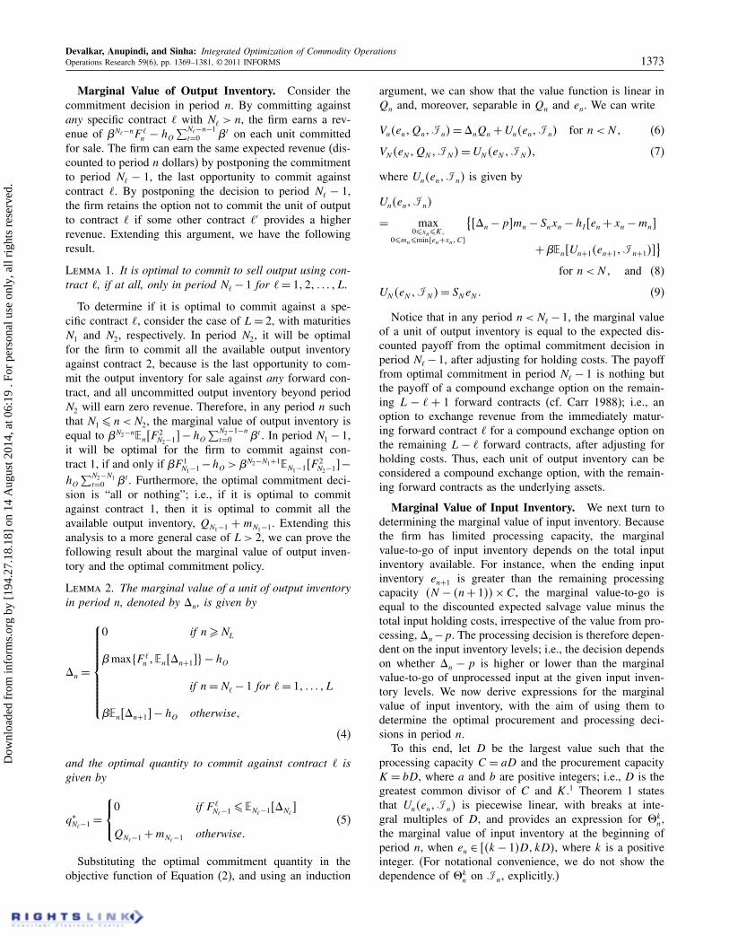
optimal procurement and processing policy is governedby two price-, and horizon-dependent inventory thresholds,snD and rnD. To compare these thresholds, it is useful torestate the optimal processing policy, obtained by substitut-ing the optimal procure up to level given by Equation (16)into Equation (13) as follows:
m∗
n =
C if ì4k5n <ãn −p
min84y∗n − rnD5+1C9
if ì4k5n ¾ãn −p¾ì4k+b5
n
0 if ì4k+b5n >ãn −p1
(17)
where rn = max8r ∈+ ∪ 809 s.t. ì4r5n >ãn −p9.
Consider the situation when the “processing margin”from procuring and processing is negative; i.e., ãn − p −
Sn ¶ 0. Any procurement in the current period is beneficialonly if the expected marginal value-to-go of the procuredunit is greater than Sn. Similarly, it is optimal to processwhenever the benefit from processing, ãn − p, is greaterthan the expected marginal value-to-go. By concavity of thevalue function, snD ¶ rnD and the starting inventory levelcan be divided into three regions: (a) en ∈ 601 snD5, where itis optimal to only procure input; (b) en ∈ 6snD1 rnD7, whereit is optimal to neither procure nor process any input, and(c) en ∈ 4rnD15, where it is optimal to only process theinput. The optimal procurement and processing quantitiesare given by x∗
n = y∗n −en = min8K1 4snD−en5
+9 and m∗n =
min8C1 4en − rnD5+9. It is important to notice that eventhough the processing margin is negative, it is still optimalto process when the input inventory is sufficiently high.On the other hand when the processing margin is positive,i.e., ãn − p − Sn > 0, there is benefit from procuring andprocessing the input immediately. Thus, for some startinginput inventory levels, it might be optimal to both procureand process the input. This fact makes it difficult to dividethe starting input inventory level into mutually exclusiveregions where only one of the actions, procurement or pro-cessing, is optimal. At least one of the two activities isat capacity for all starting inventory levels and both pro-curement and processing of the input are optimal for someinventory levels.
We illustrate the features of the optimal policy using anexample. To make the intuition clear, and keep the exposi-tion simple, we consider a three-period problem with deter-ministic prices, no holding costs and = 1.
Example. Consider the situation where K =C and theoutput commodity prices are such that ã1 − p = ã2 − p ≡
ã−p. The input spot prices in periods 1 and 2 and the sal-vage value in period 3 are such that S3 <S1 <ã−p < S2.
Now, consider the procurement decision in period 1.Because S1 <ã1 − p, it is optimal for the firm to procureinput to meet period 1’s processing requirements. BecauseS1 < ã2 − p < S2, it is optimal to procure for period 2’sprocessing requirements in period 1 itself. Finally, becauseS1 > S3, it is not optimal to procure for salvaging at theend of the horizon. The total quantity that can be pro-cessed over periods 1 and 2 is equal to 2C, and thereforethe optimal procurement quantity in period 1 is given byx∗
1 = min8K1 42C − e15+9.
In this example, we have a = b = 1 and D = C. UsingEquations (11) and (10), we can calculate ì
4151 = ì
4251 =
ã − p and ì4k51 = S3 for k ¾ 3. We see that s1D = 2D
for period 1. The optimal procurement quantity in period 1is therefore given by x∗
1 = y∗1 − e1 = min8K1 42C − e15
+9,corresponding to the different cases in Equation (16).
The benefit from processing is identical in periods 1and 2 and greater than the salvage value. Thus, it is optimal
for the firm to process all the available input inventory-up-to processing capacity. The optimal processing quantity inperiod 1 is thus given by m∗
1 = min8C1 e1 +x∗19. We see that
r1D = 0, and the optimal processing quantity correspondsto the second case in Equation (17).
Figure 1 illustrates the optimal procurement and pro-cessing quantities in period 1, along with ì
4k51 values for
different starting inventory levels.
3.2. Multiple Output Commodities
In reality, multiple output commodities could be producedupon processing the input; e.g., soybean is crushed to pro-duce soybean meal and oil, both of which are commoditiesthat can be traded. The results obtained in the previoussection can be extended to the case when multiple out-put commodities are produced upon processing the input.To keep the exposition simple, we illustrate the case whentwo products are produced upon processing the input; theextension to more products is straightforward.
Let one unit of input, when processed, yield M unitsof product M and O units of product O, with M and O
nonnegative and 0 < M + O ¶ 1 (one could think of Mand O to denote meal and oil in the soybean processingcontext). Let `m and `o index the forward contracts avail-able for output M and O, respectively, with maturity atN`m
and N`o. Let M `m
n and O`On be the forward prices on
these contracts. Let hM and hO be the unit holding cost perperiod for M and O.
After processing, the decision to commit commodity Mor O for sale against a forward contract can be made inde-pendent of the decision for the other commodity, becausethere are no capacity constraints on the commitment deci-sion itself. Thus, similar to the single output case, theoptimal commitment policy for each output commodity isgiven by Lemma 1. Also, the marginal value of inventoryfor output j , denoted by ã4j5
n , is given by Equation (4).The expected benefit from processing in period n is there-fore equal to
∑
j=M1O jã4j5n − p. The marginal value of
input inventory, optimal procurement and processing pol-icy are given by Equations (10), (16), and (17), with ãn =∑
j=M1O jã4j5n .
4. Numerical StudyIn this section, we illustrate our analytical results usingnumerical studies. We consider the soybean procurementand processing decisions as the context and use commoditymarket data for the soy complex for our numerical studies.
While the analytical results derived in §3 did not dependon the specific dynamics of the various commodity prices,computing the marginal values and optimal policy param-eters does depend on the specific price processes. Single-factor mean-reverting price processes have often been usedto model the spot price processes for various commodi-ties, including agricultural commodities (cf. Geman 2005,Chapter 3). These models capture an essential feature ofcommodity spot prices, which is that commodity pricestend to revert to a mean level. An attractive feature of thesingle-factor mean-reverting price processes is their ana-lytical tractability. While other multi-factor price processesare also used to model commodity prices (see discussionat the end of this section), in this section we model thevarious commodity prices as single-factor mean-revertingprocesses and demonstrate the computation of the opti-mal policy using binomial lattices to model the joint evo-lution of the commodity prices. We compare the perfor-mance of the optimal policy (described in §§3.1 and 3.2)with that of heuristics used in practice and the option val-uation literature. Specifically, we consider two heuristics:(a) modeling multiple outputs produced upon processingas a single, composite product to determine the input pro-curement and processing policies; and (b) a myopic, fullcommitment policy that uses the net margin from process-ing and committing all the output immediately to determinethe procurement and processing decisions.
4.1. Implementation
Modeling the Commodity Price Processes. We usea single-factor mean-reverting price process as in Jailletet al. (2004) to describe the evolution of the spot pricesof the various commodities under the risk-neutral measure.Specifically, Si4t5, the spot price of commodity i at time t ismodeled as lnSi4t5= i4t5+4t5, where i4t5 is the loga-rithm of the deseasonalized price and 4t5 is a determinis-tic factor which captures the seasonality in spot prices. Thedeseasonalized price i4t5 follows a mean-reverting processgiven by di4t5 = i4i − i4t55dt + idWi4t5 where i isthe mean-reversion coefficient, i is the long-run log pricelevel, i is the volatility, and dWi4t5 is the increment of astandard Brownian motion.
Data and Estimation of the Price Process Param-eters. The parameters of the spot price process underthe risk-neutral measure can be estimated by calibratingthem to the observed futures prices for the various com-modities, as described in Jaillet et al. (2004). Specifically,the futures price at time t for delivery at T ¾ t is given
by Fi4t1 T 5= Ɛ6Si4T 5 I4t57, where denotes the risk-neutral probability measure, and we have
lnFi4t1 T 5=4T 5+ 41 − e−i4T−t55i + e−i4T−t5i4t5
+2i
4i
61 − e−2i4T−t570
The futures price information on futures contracts tradedon the Chicago Board of Trade (CBOT) for different matu-rities on each trading day of the month of June 2010 wasused to calibrate the parameters for soybean, soybean meal,and soybean oil spot price processes. Futures contracts withthe nearest 9 maturities for soybean, nearest 13 maturitiesfor soybean meal, and nearest 12 maturities for soybean oilwere used for the calibration. While contracts with furthermaturities are traded for each commodity, these contractswere not included in the calibration because they had verylittle trading volume on each of the trading days used inthe sample. For each trading day, the parameters were esti-mated by minimizing the sum of the absolute deviationsbetween the actual and estimated futures prices for variousmaturities.
The minimization was carried out by approximatingthe seasonality factors to be constant between differentmaturity months in a year and imposing a normalizationconstraint such that
∑t=12t=1 4t5 = 0. In addition, we also
impose the constraint that the estimated 30-day and 60-dayvolatilities match the implied volatility information for eachcommodity. The implied volatility is the volatility impliedby the market price of the option based on an option pricingmodel, and these data were obtained from the Bloombergservice. The average of the estimated parameters obtainedover each trading day are given in Table 1 and are used tomodel the price processes. The standard errors for the keyparameters and root mean-squared errors (RMSE) betweenthe observed and estimated prices for each commodity aregiven in Table 2.
Table 1. Price process parameters.
Soybean Soybean meal Soybean oil
Mean-reversion coeff i 0.229 0.656 0.399Longrun log level i 6.738 5.500 3.734Volatility i 0.244 0.270 0.233Seasonality factor e4t5
Mean-reversion coeff i 000310 000252 000049Longrun log level i 000028 000035 000032Volatility i 000006 000005 000002RMSE (% terms) (%) 1040 2015 1058
The various commodities are related through input-output processes, and the underlying uncertainty in theirprice processes are likely to be correlated. We estimated thecorrelation between the Brownian motion increments forthe three commodities using historical weekly returns onthe nearest maturing futures contracts over the time period1/1/2000–12/31/2009. The estimated correlations are givenin Table 3.
Computation of the Optimal Policy. For computingthe optimal policy, we use the re-combining binomialtree procedure described in Peterson and Stapleton (2002),which can handle mean reversion in prices, to discretizethe dynamics of the price processes and approximate thejoint evolution of the spot price of the various commodi-ties. Each period in the discrete binomial tree correspondsto a week, and we discretize the price process with steps between each period. In our computational studies,we set = 5. We have 64n − 15 + 17J nodes in the treefor period n, where J is the total number of commodi-ties whose joint price evolution is approximated. At eachnode in the tree, we can compute the forward price F `
n
for l = 1121 0 0 0 1L for each output commodity using thediscrete transition probabilities at that node. Finally, usingEquations (4) and (10), we can compute ãn for each out-put and äk
n for k = 11 0 0 0 1 4N − n5a + 1, and thereby theprocurement and processing policy at each node in the tree.
We evaluate the performance of this policy using MonteCarlo simulation. We generate sample paths of prices foreach period n= 1121 0 0 0 1N by sampling from the continu-ous time price process for the commodities. We round therealized input and output spot prices to the closest nodein the binomial tree and obtain the procurement, process-ing, and commitment quantity corresponding to the nodeand inventory level. Expected profits from the policy arecomputed as the average profit over 10,000 sample paths.All the numerical studies were conducted using MATLAB(version 7.9.0 R2009b) software on a Dell Optiplex 755with E8400 3.00 GHz Intel Core2 Duo CPU and 2 GBRAM, running Windows Vista Enterprise.
While we refer to the policy computed above as the opti-mal policy, it is optimal only if the various commodity
prices evolve as the binomial lattices. In reality, the bino-mial lattice is an approximation of the true, continuous timeand space price processes, and strictly speaking, the policyis only an optimization-based policy (our numerical exper-iments indicate that the gap between the value of the pol-icy computed using lattices and the value estimated usingMonte Carlo simulation is small enough that making thisdistinction is not important).
Other Operational Parameters. For all the numericalstudies, we set the variable cost of processing p to equal72 cents/bushel, which corresponds to about 35% of thegross margin from processing one bushel of soybean, basedon the long-run average prices of the three commodities.This value of the processing cost is close to the averageprocessing costs estimated for the U.S. soybean processingindustry (Soyatech 2008). The procurement and process-ing capacities are set to 5 and 3 units, respectively. Thesecapacities can be considered to be in multiples of bushels,e.g., million bushels. For the base case, we set processingcapacity to 60% of total procurement capacity, which isroughly the percentage of soybeans produced in the UnitedStates that were estimated to have been crushed in 2008and 2009 (Ash 2011). We leave the exact units for thecapacities unspecified because only the relative values ofthe procurement and processing capacities matter for com-puting the policies, and multiplying both the capacities bya common factor will scale the expected profits also bythe same factor. We assume the physical holding costs forthe various commodities are negligible and normalize themto zero.
4.2. Numerical Results
We conduct numerical studies to compute the expectedprofits for the firm from its procurement and process-ing operations over the procurement season ranging fromAugust to December. We initialize the prices for all thecommodities to their long run average values at the begin-ning of the planning horizon and evaluate the performanceof the policy for different horizon lengths. Table 4 givesthe optimal expected profits for different horizon lengthswhen the firm uses all forward contracts available over thehorizon for each output commodity.
The optimal policy above is obtained by modeling thejoint evolution of the input and individual output commod-ity prices and using the results in §3.2. The number ofnodes in the binomial tree used to represent the joint evo-lution of commodity prices increases exponentially withthe number of output commodities. Thus, the computa-tional complexity increases quickly as the number of outputcommodities increases, requiring one to consider tractableapproximations.
Composite Output Approximation. A potentialapproach to compute heuristic policies when multipleoutput commodities are produced is to model all theoutputs together as a single “composite” product and
Table 4. Optimal expected profits for different horizonlengths.
Number of OptimalHorizon forward contracts L expected profits Avg. CPU timelength N (maturities N`) (std. error) (in sec.)
5 1 11557065 8068(5) 40033%5
10 2 31095066 20607445195 40044%5
20 3 61954021 4128403945191185 40069%5
model the price process for this composite product. Thisis similar to the approach used by Borovkova et al. (2007)in the valuation of basket options, i.e., options on a linearcombination of different assets, where the entire basket ofcommodities is modeled as a single “composite” product.We model a hypothetical composite output whose pricein any period is equal to the total value of soybean mealand soybean oil produced upon processing one bushelof soybeans, where the value is calculated based on thecurrent prices of the two products. Because only futuresinstruments are publicly traded for the different outputcommodities, we consider futures instruments for thecomposite output as well, where the futures price for aparticular maturity is a combination of the futures pricesof the individual output commodities, to estimate theprice process parameters for the composite output. Theparameters of the price process for the composite outputcan be estimated as described in §4.1 by considering thehypothetical futures instruments for the composite output.The joint evolution of the input and composite output canbe modeled using a binomial tree and a heuristic policycomputed using the results for the single output case in§3.1. This heuristic yields a feasible policy for the originalmodel with separate output commodities and the totalexpected profits from following such a heuristic policy,and the gap with respect to the optimal expected profitsfor different horizon lengths, are shown in Table 5.2
As seen from Table 5, approximating the multiple out-puts as a single composite output comes with very littleloss in optimality. The composite output approximation isalso computationally far less burdensome than the optimalpolicy, as seen from the CPU times.
The composite output approximation, in addition toapproximating the joint evolution of two output commod-ity prices as a single composite price, also leads to a lowerflexibility in the commitment decision for the two outputproducts. This is because when the composite output iscommitted for sale against a forward contract, both theunderlying output products are committed for sale againsttheir respective forward contracts, maturing in the sameperiod. This is not necessarily the case under the optimalpolicy, where the commitment decisions for the individ-ual outputs are independent of each other. The results in
Table 5. Expected profits using composite outputapproximation.
Number of Expected Gap (as % Avg. CPUHorizon forward contracts L profits of optimal) timelength N (maturities N`) (std. error) (%) (in sec.)
5 1 11557071 000† 1017(5) 40033%5
10 2 31061071 1010 1108945195 40046%5
20 3 61917071 0052 11204845191185 40069%5
†p-value> 001.
Table 5 imply that the loss in value by ignoring this flex-ibility in commitment is negligible. Furthermore, the lossin information because of approximating the outputs by asingle product has negligible impact on the total expectedprofits.
Full Commitment Policy. We evaluate the benefit offollowing an optimal policy by comparing the optimalexpected profits with the expected profits from following amyopic policy, which considers only the value from pro-cessing and committing the output immediately in the sameperiod. Under this myopic policy, termed the full com-mitment policy, the firm procures up to the minimum ofprocurement and processing capacities if there exists a pos-itive margin from processing and committing the outputimmediately, and nothing otherwise. Notice that full com-mitment policy ignores the “option” value from postponingcommitment of the output, as also the value from holdingand trading the input inventory at the end of the horizon.The expected profits and gap, with respect to optimal prof-its from following the full commitment policy for differenthorizon lengths, are shown in Table 6.3
The results in Table 6 suggest that the benefits ofintegrated decision making are negligible compared to amyopic policy. However, these results are for the base set ofparameters and do not necessarily imply the same behaviorunder all circumstances. To investigate this issue, we con-sider sensitivity of the different policies to two key param-eters: processing capacity and price volatilities.4
Table 6. Expected profits from full commitment policy.
Number of ExpectedHorizon forward contracts L profits Gap (as % oflength N (maturities N`) (std. error) optimal) (%)
5 1 11563056 −0038†
(5) 400110510 2 31106067 −0036†
45195 400160520 3 61829088 1079
45191185 4002305
†p-value> 001.
Impact of Processing Capacity. When processingcapacity is limited compared to the procurement capacity,we expected the value of integrated decision making to behigher. This is because when the input spot prices are low,the optimal policy is likely to procure input for currentperiod processing as well as for the future. The myopicpolicy, however, does not do so. Furthermore, including theoption to trade input inventory at the end of the horizonis more valuable when processing capacity is limited. Theresults in Table 7, which shows the expected profits underthe three policies as the processing capacity is varied from20% to 100% of the procurement capacity, support thisintuition.
Compared to a myopic policy, the benefits from usingthe optimal policy can be as high as 9.4% for highly con-strained processing firms and reduces as the processingcapacity increases (the negative value in the last row is sta-tistically insignificant). On the other hand, we notice thatthe gap between the optimal profits and the profits usingthe composite output approximation increases with the pro-cessing capacity, because more of the input procured isprocessed and sold as output. Thus, the loss in flexibility tocommit the different outputs to contracts maturing at dif-ferent dates has a higher impact. However, the maximumgap, at 2.5%, is still low.
Impact of Price Volatilities. All three policies—fullcommitment, composite output, and optimal—have option-like features. While the full commitment policy is equiva-lent to the exercise of a European spread option betweenthe output and input prices, the composite output andoptimal policies model the output commitment decisionas a compound exchange option, in addition to modelingthe procurement and processing decisions based on spreadoptions. Given this, the expected profits under each pol-icy increase with commodity price volatilities, as seen inTable 8.
We also notice that the gap between the optimal policyand the full commitment policy increases as the volatil-ity increases. This is because the full commitment policymodels the marginal value of output based on the real-ized output prices and does not account for the exchangeoption inherent in the output commitment decision. Fur-thermore, the full commitment policy does not procureadditional input in periods with low input spot price forprocessing needs in future periods. The value of this oppor-tunistic input procurement also increases as price volatilityincreases.
In summary, approximating multiple outputs using ahypothetical single composite output product is near-optimal and captures almost the entire value from followingan optimal policy. The value of integrated decision makingcan be significant for firms with tight processing capacitiesfacing high commodity price volatility.
While single factor, mean-reverting processes are goodapproximations for modeling commodity price processes,
they also have drawbacks. For instance, under a singlefactor, mean-reverting process, the volatility of futuresprices decreases exponentially to zero as time to maturityincreases. To overcome these drawbacks and explain otherempirical features of commodity prices, various multi-factor models have also been proposed to model differ-ent commodity prices (see, for instance, Schwartz andSmith 2000, Geman and Nguyen 2005). While these mod-els provide a better description of the price processes, theycome with added computational complexity. Computingthe optimal policy is difficult because modeling the jointevolution of these multi-factor price processes becomescomputationally inefficient (the number of nodes in the lat-tice increases exponentially with the number of factors). Asa result, one has to resort to tractable heuristics. We dis-cuss one particular heuristic to address these computationalchallenges. Details of the heuristic, along with the compu-tation of an upper bound against which the heuristic can becompared, and numerical illustrations can be found in theonline appendix.
5. ConclusionIn this paper, we have considered the integrated procure-ment, processing, and trade decisions for a firm dealingin commodities and subject to procurement and processingconstraints. We solved the problem optimally and showedthat the procurement and processing decisions in any periodare governed by price-dependent inventory thresholds. Wedeveloped recursive expressions to computes these thresh-olds and illustrate our analytical results using commodity
markets data for the soybean complex. Through numericalstudies, we find that approximating multiple outputs pro-duced upon processing (e.g., soybean meal and oil) by asingle, composite output product is near-optimal. Integrateddecision making provides significant benefits compared toa myopic policy, which considers only the benefit from pro-cessing and trading the output immediately. The value ofintegrated decision making is especially high under condi-tions of tight processing capacities and high price volatili-ties. We also propose a computationally tractable heuristicfor computing procurement and processing decisions whencommodity prices are driven by multi-factor processes.
The results in the current paper can easily be extendedto incorporate convex piecewise linear procurement costsand/or concave piecewise linear salvage values for the inputinventory. Furthermore, input trade opportunities through-out the horizon can also be easily incorporated into theanalysis.
Our work lays the foundation for further research incommodity processing and trading operations. Typically,commodity processors operate networks, with procurementand processing activities spread across multiple locations.For instance, the ITC e-Choupal network has multipleprocurement hubs, along with a few central processinglocations. While commodity production and distributionnetworks have been studied earlier (cf. Markland 1975,Markland and Newett 1976), these papers assume deter-ministic commodity prices and no operational constraints.It will be an interesting research topic to extend our modelsto a network setting, incorporating stochastic commodityprices and operational constraints.
6. Electronic CompanionAn electronic companion to this paper is available as partof the online version that can be found at http://or.journal.informs.org/.
Endnotes1. Technically, a greatest common divisor may not exist ifeither C or K is not a rational number. We assume C andK are both rational.2. Unless indicated, the gaps shown in all tables are sig-nificant with p < 0005.3. The negative gaps are because the optimal policy iscomputed assuming the various commodities prices evolvein discrete space and time, while the performance of thepolicies are evaluated using a Monte Carlo simulation thatsamples from the continuous time and space price pro-cesses. As indicated, the negative values for the gaps arestatistically insignificant. The same explanation also holdsfor negative gaps seen in Tables 7 and 8.4. We also ran sensitivity analysis by varying the correla-tion between the different price processes. For various val-ues of the correlation factors, we observed gaps that rangedfrom 0.85% to 1.32%.
AcknowledgmentsThe authors gratefully acknowledge the collaboration andsupport of the ITC Group. Their generous hospitality andaccess to key personnel greatly enhanced this research. Theauthors thank the associate editor and the referees, whosemany suggestions helped improve this paper significantly.
ReferencesAnupindi, R., S. Sivakumar. 2007. Supply chain re-engineering in agri-
business: A case study of ITC’s e-choupal. H. L. Lee, C.-Y. Lee, eds.Building Supply Chain Excellence in Emerging Economies. Elsevier-Springer, New York.
Ash, M. 2011. Oil crops outlook. Electronic Report from the EconomicResearch Service, Report OCS-11b, United States Department ofAgriculture, Washington, DC.
Bellman, R. 1956. On the theory of dynamic programming—A warehous-ing problem. Management Sci. 2(3) 272–275.
Bjork, T. 2004. Arbitrage Theory in Continuous Time. Oxford UniversityPress, New York.
Borovkova, S., F. J. Permana, H. V. D. Weide. 2007. A closed formapproach to the valuation and hedging of basket and spread option.J. Derivatives 14(4) 8–24.
Brown, D. B., J. E. Smith, P. Sun. 2010. Information relaxations andduality in stochastic dynamic programs. Oper. Res. 58(4) 785–801.
Carr, P. 1988. The valuation of sequential exchange opportunities.J. Finance 43(5) 1235–1256.
Charnes, A., J. Dreze, M. Miller. 1966. Decision and horizon rules forstochastic planning problems: A linear example. Econometrica 34(2)307–330.
Deng, S. J., B. Johnson, A. Sogomonian. 2001. Exotic electricity optionsand the valuation of electricity generation and transmission assets.Decision Support Systems 30(3) 383–392.
Dreyfus, S. E. 1957. An analytic solution of the warehouse problem. Man-agement Sci. 4(1) 99–104.
Geman, H. 2005. Commodities and Commodity Derivatives: Modeling andPricing for Agriculturals, Metals and Energy. John Wiley & Sons,West Sussex, UK.
Geman, H., V. Nguyen. 2005. Soybean inventory and forward curvedynamics. Management Sci. 51(7) 1076–1091.
Hull, J. C. 1997. Options, Futures and Other Derivatives. Prentice Hall,Upper Saddle River, NJ.
Jaillet, P., E. I. Ronn, S. Tompaidis. 2004. Valuation of commodity-basedswing options. Management Sci. 50(7) 909–921.
Keppo, J. 2004. Pricing of electricity swing options. J. Derivatives 11(3)26–43.
Lai, G., F. Margot, N. Secomandi. 2010. An approximate dynamic pro-gramming approach to benchmark practice-based heuristics for natu-ral gas storage valuation. Oper. Res. 58(3) 564–582.
Lai, G., M. X. Wang, S. Kekre, A. Scheller-Wolf, N. Secomandi. 2011.Valuation of storage at a liquefied natural gas terminal. Oper. Res.59(3) 602–616.
Markland, R. E. 1975. Analyzing multi-commodity distribution net-works having milling-in-transit features. Management Sci. 21(12)1405–1416.
Markland, R. E., R. J. Newett. 1976. Production-distribution planningin a large scale commodity processing network. Decision Sci. 7(4)579–594.
Martınez-de Albéniz, V., J. M. V. Simón. 2010. A capacitated commoditytrading model with market power. Working paper, IESE BusinessSchool, University of Navarra, Barcelona, Spain.
Nascimento, J. M., W. B. Powell. 2009. An optimal approximate dynamicprogramming algorithm for the lagged asset acquisition problem.Math. Oper. Res. 34(1) 210–237.
Peterson, S. J., R. C. Stapleton. 2002. The pricing of Bermudan-styleoptions on correlated assets. Rev. Derivatives Res. 5(2) 127–151.
Plato, G. 2001. The soybean processing decision: Exercising a realoption on processing margins. Electronic Report from the EconomicResearch Service, Technical Bulletin Number 1897, United StatesDepartment of Agriculture, Washington, DC.
Prahalad, C. K. 2005. Fortune at the Bottom of the Pyramid. WhartonSchool Publishing, Philadelphia.
Routledge, B. R., D. J. Seppi, C. S. Spatt. 2001. The spark spread: Anequilibrium model of cross-commodity price relationships in elec-tricity. Working paper, Tepper School of Business, Carnegie MellonUniversity, Pittsburgh.
Schwartz, E., J. E. Smith. 2000. Short-term variations and long-termdynamics in commodity prices. Management Sci. 46(7) 893–911.
Secomandi, N. 2010a. On the pricing of natural gas pipeline capacity.Manufacturing Service Oper. Management 12(3) 393–408.
Secomandi, N. 2010b. Optimal commodity trading with a capacitated stor-age asset. Management Sci. 56(3) 449–467.
Soyatech. 2008. How the global oilseed and grain trade works. Reportprepared for U.S. Soybean Export Council and United SoybeanBoard by HighQuest Partners and Soyatech. Soyatech, SouthwestHarbor, ME.
Tseng, C. L., G. Barz. 2002. Short-term generation asset valuation: A realoptions approach. Oper. Res. 50(2) 297–310.
Tseng, C. L., K. Y. Lin. 2007. A framework using two-factor price latticesfor generation asset valuation. Oper. Res. 55(2) 234–251.
Wu, O. Q., H. Chen. 2010. Optimal control and equilibrium behavior ofproduction-inventory systems. Management Sci. 56(8) 1362–1379.


![Commodities COMMODITIES BULLETIN - HFW | Bulletin [A4 4pp] July 2012.pdf · Commodities Bulletin 03…](https://static.documents.pub/doc/80x56/5b5eec517f8b9a057e8d30dd/commodities-commodities-bulletin-hfw-bulletin-a4-4pp-july-2012pdf-commodities.jpg)


