Integration of Bridge Damage Detection Concepts and Components

Final Report 1 of 3October 2013

Sponsored byIowa Highway Research Board(IHRB Project TR-636)Iowa Department of Transportation(InTrans Project 11-416)

Volume I: Strain-Based Damage Detection

About the BEC

The mission of the Bridge Engineering Center is to conduct research on bridge technologies to help bridge designers/owners design, build, and maintain long-lasting bridges.

Disclaimer Notice

The contents of this report reflect the views of the authors, who are responsible for the facts and the accuracy of the information presented herein. The opinions, findings and conclusions expressed in this publication are those of the authors and not necessarily those of the sponsors.

The sponsors assume no liability for the contents or use of the information contained in this document. This report does not constitute a standard, specification, or regulation.

The sponsors do not endorse products or manufacturers. Trademarks or manufacturers’ names appear in this report only because they are considered essential to the objective of the document.

Non-Discrimination Statement

Iowa State University does not discriminate on the basis of race, color, age, religion, national origin, sexual orientation, gender identity, genetic information, sex, marital status, disability, or status as a U.S. veteran. Inquiries can be directed to the Director of Equal Opportunity and Compliance, 3280 Beardshear Hall, (515) 294-7612.

Iowa Department of Transportation Statements

Federal and state laws prohibit employment and/or public accommodation discrimination on the basis of age, color, creed, disability, gender identity, national origin, pregnancy, race, religion, sex, sexual orientation or veteran’s status. If you believe you have been discriminated against, please contact the Iowa Civil Rights Commission at 800-457-4416 or Iowa Department of Transportation’s affirmative action officer. If you need accommodations because of a disability to access the Iowa Department of Transportation’s services, contact the agency’s affirmative action officer at 800-262-0003.

The preparation of this report was financed in part through funds provided by the Iowa Department of Transportation through its “Second Revised Agreement for the Management of Research Conducted by Iowa State University for the Iowa Department of Transportation” and its amendments.

The opinions, findings, and conclusions expressed in this publication are those of the authors and not necessarily those of the Iowa Department of Transportation.

Technical Report Documentation Page

1. Report No. 2. Government Accession No. 3. Recipient’s Catalog No.

IHRB Project TR-636

4. Title and Subtitle 5. Report Date

Integration of Bridge Damage Detection Concepts and Components

Volume I: Strain-Based Damage Detection

October 2013

6. Performing Organization Code

7. Author(s) 8. Performing Organization Report No.

Brent M. Phares, Lowell Greimann, and Hyungjoo Choi InTrans Project 11-416

9. Performing Organization Name and Address 10. Work Unit No. (TRAIS)

Bridge Engineering Center

Iowa State University

2711 South Loop Drive, Suite 4700

Ames, IA 50010-8664

11. Contract or Grant No.

12. Sponsoring Organization Name and Address 13. Type of Report and Period Covered

Iowa Highway Research Board

Iowa Department of Transportation

800 Lincoln Way

Ames, IA 50010

Final Report 1 of 3

14. Sponsoring Agency Code

IHRB Project TR-636

15. Supplementary Notes

Visit www.intrans.iastate.edu for color pdfs of this and other research reports.

16. Abstract

In this work, a previously-developed structural health monitoring (SHM) system was advanced toward a ready-for-

implementation system. Improvements were made with respect to automated data reduction/analysis, data acquisition hardware,

sensor types, and communication network architecture.

The statistical damage-detection tool, control-chart-based damage-detection methodologies, were further investigated and

advanced. For the validation of the damage-detection approaches, strain data were obtained from a sacrificial specimen attached to

the previously-utilized US 30 Bridge over the South Skunk River (in Ames, Iowa), which had simulated damage,. To provide for

an enhanced ability to detect changes in the behavior of the structural system, various control chart rules were evaluated. False

indications and true indications were studied to compare the damage detection ability in regard to each methodology and each

control chart rule.

An autonomous software program called Bridge Engineering Center Assessment Software (BECAS) was developed to control all

aspects of the damage detection processes. BECAS requires no user intervention after initial configuration and training.

17. Key Words 18. Distribution Statement

assessment software—BECAS—control chart based—damage-detection

methodology—false-indication rate—SHM—structural health monitoring—

true-indication rate

No restrictions.

19. Security Classification (of

this report)

20. Security Classification (of this

page)

21. No. of Pages 22. Price

Unclassified. Unclassified. 79 NA

Form DOT F 1700.7 (8-72) Reproduction of completed page authorized

THREE-VOLUME REPORT ABSTRACT

The Iowa Department of Transportation (DOT) started investing in research (through both the

Iowa Highway Research Board and the Office of Bridges and Structures) in 2003 to develop a

structural health monitoring (SHM) system capable of identifying damage and able to report on

the general operational condition of bridges. In some cases, the precipitous for these

developments has been a desire to avoid damage that might go unnoticed until the next biennial

inspection. Of specific and immediate concern was the state’s inventory of fracture-critical

structures.

The goal of this project was to bring together various components of recently-completed research

at Iowa’s Regent Universities with the following specific objectives:

Final development of the overall SHM system hardware and software

Integration of vibration-based measurements into current damage-detection algorithm

Evaluation and development of energy-harvesting techniques

The three-volume final report summarizes the results of this project as follows:

Volume I: Strain-Based Damage Detection, from the Iowa State University Bridge

Engineering Center, reviews information important to the strain-based SHM methodologies,

details the upgraded damage-detection hardware and software system, demonstrates the

application of the control-chart-based methodologies developed, and summarizes the results in

graphical and tabular formats.

Volume II: Acceleration-Based Damage Detection, from the University of Iowa Center for

Computer-Aided Design, presents the use of vibration-based damage-detection approaches as

local methods to quantify damage at critical areas in structures. Acceleration data were collected

and analyzed to evaluate the relationships between sensors and with changes in environmental

conditions. A sacrificial specimen was investigated to verify the damage-detection capabilities

and this volume presents a transmissibility concept and damage-detection algorithm that show

potential to sense local changes in the dynamic stiffness between points across a joint of a real

structure.

Volume III: Wireless Bridge Monitoring Hardware, from the University of Northern Iowa,

Electrical Engineering Technology, summarizes the energy harvesting techniques and prototype

development for a bridge monitoring system that uses wireless sensors. The functions and

performance of the developed system, including strain data, energy harvesting capacity, and

wireless transmission quality, are covered in this volume.

INTEGRATION OF BRIDGE DAMAGE DETECTION

CONCEPTS AND COMPONENTS

VOLUME I: STRAIN-BASED DAMAGE DETECTION

Final Report 1 of 3

October 2013

Principal Investigator

Brent M. Phares, Director

Bridge Engineering Center, Iowa State University

Co-Principal Investigators

Salam Rahmatalla, Associate Professor

Civil and Environmental Engineering, Center for Computer-Aided Design, University of Iowa

Jin Zhu, Associate Professor

Electrical Engineering Technology, University of Northern Iowa

Ping Lu, Rating Engineer

Office of Bridges and Structures, Iowa Department of Transportation

Research Assistant

Hyungjoo Choi

Authors

Brent M. Phares, Lowell Greimann, and Hyungjoo Choi

Sponsored by

the Iowa Highway Research Board and Iowa Department of Transportation

(IHRB Project TR-636)

Preparation of this report was financed in part

through funds provided by the Iowa Department of Transportation

through its Research Management Agreement with the

Institute for Transportation

(InTrans Project 11-416)

A report from

Institute for Transportation

Iowa State University

2711 South Loop Drive, Suite 4700

Ames, IA 50010-8664

Phone: 515-294-8103 Fax: 515-294-0467

www.intrans.iastate.edu

v

TABLE OF CONTENTS

ACKNOWLEDGMENTS ............................................................................................................. ix

EXECUTIVE SUMMARY ........................................................................................................... xi

1. INTRODUCTION .......................................................................................................................1

1.1 General Background ......................................................................................................1 1.2 Objective of Research ....................................................................................................1 1.3 Organization of Report ..................................................................................................2

2. PERTINENT LITERATURE REVIEW......................................................................................3

2.1 Cross Prediction Model Control Chart Method .............................................................3

2.2 Methodology Validation ................................................................................................6

2.3 Orthogonal Regression and Statistical Evaluation Approach ........................................9

3. DAMAGE DETECTION HARDWARE AND SOFTWARE ..................................................13

3.1 Hardware ......................................................................................................................13 3.2 Software .......................................................................................................................17

4. DAMAGE-DETECTION METHODOLOGIES .......................................................................18

4.1 Overall Methodology ...................................................................................................18 4.2 Truck Event Control Chart Methods............................................................................20

4.3 Cross Prediction Control Chart Method ......................................................................31 4.4 F-Test Control Chart Method.......................................................................................39 4.5 Discussion ....................................................................................................................47

5. SUMMARY, CONCLUSIONS, AND RECOMMENDATIONS ............................................50

5.1 Summary ......................................................................................................................50 5.2 Conclusions ..................................................................................................................51 5.3 Recommendations for Future Work.............................................................................51

REFERENCES ..............................................................................................................................53

APPENDIX A. SPECIFICATIONS FOR THE FIBER-OPTIC SENSORS IN THE US 30

SHM SYSTEM ..................................................................................................................55

APPENDIX B. SETTING UP FTP DATA SYNCHRONIZATION PROCESS USING

BESTSYNC 2013 ..............................................................................................................57

vi

LIST OF FIGURES

Figure 2.1. Basic plan view of the US 30 Bridge ............................................................................3 Figure 2.2. Example of matched data from two sensors with applied limits (right) (Wipf et al.

2007) ....................................................................................................................................4

Figure 2.3. Sample distribution of the combined-sum-residuals (Lu 2008) ....................................5 Figure 2.4. Sample control chart (Lu 2008) .....................................................................................6 Figure 2.5. Typical installed sacrificial specimen and double curvature bending of sacrificial

specimen (Phares et al. 2011) ..............................................................................................7 Figure 2.6. Sacrificial Specimen 1 cracking (Phares et al. 2011) ....................................................7

Figure 2.7. Details for sacrificial specimen with sensor array (Phares et al. 2011) .........................8 Figure 2.8. Sacrificial Specimen 2 top web plate cracking (Phares et al. 2011) .............................8 Figure 2.9. Sample standard linear regression (left) and sample orthogonal linear regression

(right) (Phares et al. 2011) ...................................................................................................9 Figure 2.10. Example of an orthogonal line fit and an orthogonal residual ..................................10 Figure 2.11. Orthogonal fit lines for the full and reduced models .................................................11

Figure 2.12. Graphical representation of rejecting H0, no damage (left) and failing to reject

H0, damage (right) ..............................................................................................................12

Figure 3.1. SHM system components and system architecture .....................................................14 Figure 3.2. Isometric view of US 30 Bridge ..................................................................................15 Figure 3.3. Bridge plan view for sensor layout ..............................................................................15

Figure 3.4. Sensors locations within the bridge framing system ...................................................16 Figure 3.5. Sensor located on the bridge deck bottom ...................................................................16

Figure 3.6. Deck bottom sensors (left) and sensor installation sample on top flange of girder

(right) .................................................................................................................................17 Figure 4.1. Damage-detection methodology ..................................................................................18

Figure 4.2. Example of false and true indication in a control chart ...............................................20

Figure 4.3. One-truck event control charts for sacrificial Specimen 2 ..........................................23 Figure 4.4. Truck events grouped by ten control charts for sacrificial Specimen 2 ......................28 Figure 4.5. Cross prediction method flow chart ............................................................................32

Figure 4.6. Cross prediction control charts for sacrificial Specimen 2 ..........................................36 Figure 4.7. Flow chart for Fshm control chart method ....................................................................39

Figure 4.8. Fshm control chart for sacrificial Specimen 2 ...............................................................46 Figure 4.9. False- and true-detection rates with Rule 1 .................................................................48

Figure 4.10. Photograph of a potential fatigue crack in web cut-back region ...............................49 Figure 4.11. False-indication rate without cut-back web-gap region ............................................49 Figure B.1. BestSync startup .........................................................................................................57 Figure B.2. File transfer .................................................................................................................58

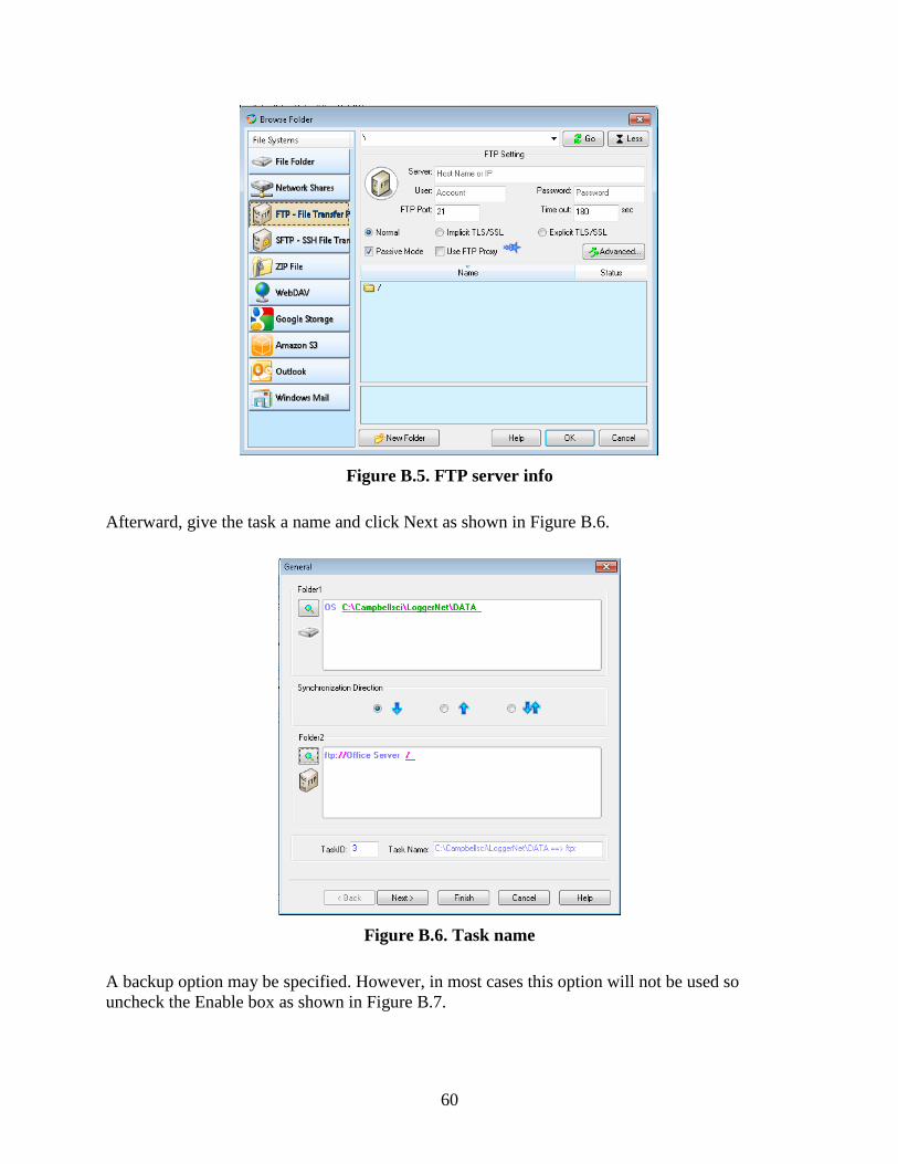
Figure B.3. Data storage location ..................................................................................................58 Figure B.4. Folder destinations ......................................................................................................59 Figure B.5. FTP server info ...........................................................................................................60

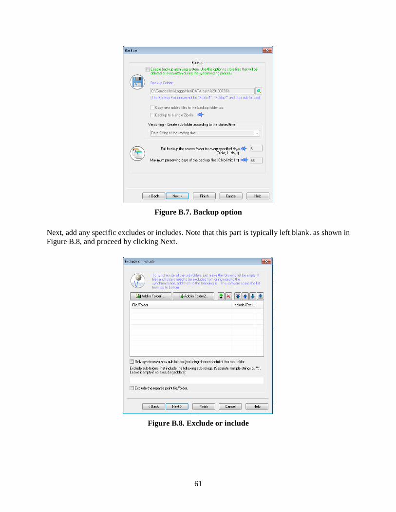
Figure B.6. Task name ...................................................................................................................60 Figure B.7. Backup option .............................................................................................................61 Figure B.8. Exclude or include ......................................................................................................61 Figure B.9. Filter files ....................................................................................................................62 Figure B.10. Copy options .............................................................................................................63

vii

Figure B.11. Volume shadow copy................................................................................................63

Figure B.12. Encryption .................................................................................................................64 Figure B.13. Naming......................................................................................................................64 Figure B.14. Speed control ............................................................................................................65

Figure B.15. Schedule real-time sync option .................................................................................65 Figure B.16. Schedule time option ................................................................................................66 Figure B.17. Log ............................................................................................................................66 Figure B.18. Application................................................................................................................67 Figure B.19. Save ...........................................................................................................................67

viii

LIST OF TABLES

Table 4.1. Control chart rules (Montogomery 1996) and number of rule checks .........................19 Table 4.2. List of select sensors used to create sample control charts ...........................................21 Table 4.3. Mean and standard deviations of select sensors for one-truck event method ...............21

Table 4.4. Rule violations for one-truck event method .................................................................24 Table 4.5. Number of false indications for sensors on bridge (non-damaged) for one-truck

event method ......................................................................................................................26 Table 4.6. Number of false and true indications for sensors on sacrificial specimen (near

damage) for one-truck event method .................................................................................26

Table 4.7. Mean and standard deviations of select sensors (µε) for truck events grouped by

ten method ..........................................................................................................................29 Table 4.8. Rule violations for truck events grouped by ten method ..............................................29

Table 4.9. Number of false indications for sensors on bridge (non-damaged) for truck events

grouped by ten method.......................................................................................................31 Table 4.10. Number of false and true indications for sensors on sacrificial specimen (near

damage) for truck events grouped by ten method ..............................................................31 Table 4.11. Mean and standard deviations of selected sensors (µε) for cross prediction

method................................................................................................................................34 Table 4.12. Rule violations for cross prediction method ...............................................................37 Table 4.13. Number of false indications for sensors on bridge (non-damaged) for cross

prediction method ..............................................................................................................38 Table 4.14. Number of false and true indications for sensors on sacrificial specimen (near

damage) for cross prediction method .................................................................................39 Table 4.15. Mean and standard deviations of select sensors (µε) for Fshm method .......................40 Table 4.16. Rule violations for Fshm control chart .........................................................................41

Table 4.17. Number of false indications for sensors on bridge (non-damaged) for Fshm

control chart .......................................................................................................................47 Table 4.18. Number of false indications for sensors on sacrificial specimen (near damage)

for Fshm control chart ..........................................................................................................47

ix

ACKNOWLEDGMENTS

The authors would like to thank the Iowa Highway Research Board (IHRB) and Iowa

Department of Transportation (DOT) for sponsoring this research. The authors would also like

the thank Ahmad Abu-Hawash and many other members of the Iowa DOT Office of Bridges and

Structures for their continued support of this research.

xi

EXECUTIVE SUMMARY

An experimental validation for an autonomous damage-detection algorithm, known as the cross

prediction methodology, was completed on the US 30 Bridge over the South Skunk River in

Ames, Iowa on a previous project. To validate the accuracy of the control-chart-based damage-

detection algorithm, sacrificial specimens were fabricated and damaged. To improve the damage

detection ability of the methodology with respect to false-indication readings a statistical f-test

was introduced.

In this work, a complete structural health monitoring (SHM) system was finalized with hardware

and software components. For example, the previously-used fiber-optic sensors were replaced

with traditional strain gauge and the external communication system was upgraded to include

automated file transfer using fourth generation (4G) cellular technology.

A complete software package named Bridge Engineering Center Assessment Software (BECAS)

was developed and includes multiple automated damage-detection processes including sensor

data acquisition, strain range data reduction, and statistical control-chart-based evaluation, based

on damage-detection methodologies. The damage detection ability was updated to include

multiple, redundant methods including: 1) one-truck event, 2) truck events grouped by ten, 3)

cross prediction, and 4) Fshm method. Each of these methods were investigated and then analyzed

in terms of false-indication rate and control chart rules.

As possibly the most intuitive damage-detection method, the one-truck event methodology

involves the construction of control charts using the strain range data for individual truck events.

For the truck events grouped by ten method, control charts are created in a similar way, but by

averaging 10 successive truck passages to create a single data point. Both the one-truck event

method and the truck events grouped by ten method had relatively low false-indication rates and

were able to detect damage. In the cross prediction and Fshm methods, the major improvement

was made in the use of orthogonal regression instead of traditional linear regression. Both

methods showed a comparatively higher number of false indications than the previous two

methods but also had significant increases in the number of true indications.

The cross prediction and Fshm methods had a relatively large number of false indications at

sensors in the cut-back web-gap region of the bridge. To have a better understanding of the cause

of the false indication, the cut-back web-gap region was inspected using visual and magnetic

particle techniques. A small crack-like indication near the cut-back web-gap region was

identified and might be actual damage detected by the system. Further study of the false-

indication rate was conducted by removing the cut-back region data.

1

1. INTRODUCTION

1.1 General Background

Bridge structural health monitoring (SHM), which typically includes specialized hardware and

software algorithms, has been widely investigated during the past two decades. Many SHM

techniques have been proposed as a means to provide methods to increase the overall safety of

bridges. These developments have been driven, in part, by a desire to have continuous feedback

on system performance that provides for a more reliable and robust transportation system. In

addition, it has been shown that periodic visual inspections may not be as reliable as desired (Lu

2008).

Since 2003, strain-based damage-detection algorithms for the US 30 Bridge over the South

Skunk River in Ames, Iowa have been studied and developed by the Iowa State University

Bridge Engineering Center. For the first generation of the damage-detection algorithm, a long-

term monitoring system was developed that included novel data management processes

including automated data zeroing, filtering, and extrema identification (Doornink 2006).

To improve the detection capabilities and to remove user subjectivity, two important

advancements were made in a second-generation system. First, a powerful vehicle-identification

system was developed and, second, the algorithm was quantified statistically. The statistical-

based damage-detection methodology, named the cross prediction method (using control chart)

was formulated by Lu (2008).

In 2010, an experimental validation was conducted to study the efficacy of the approaches.

Sacrificial specimens were mounted to an in-service bridge and exposed to real traffic loads with

fatigue cracks and thickness loss damage induced (Phares et. al 2011). The results showed that

the damage-detection algorithm detects structural damage well. Unfortunately, a relatively high

false-indication rate was also observed. Therefore, improvements to the algorithm were

investigated and evaluated. The statistical f-test was proposed as a means to improve overall

system performance (Phares et. al 2011).

In the work summarized herein, the damage-detection process based on statistical control charts,

using continuous strain range data, was further developed. False-indication and true-indication

rates were more fully investigated and then compared. The previous SHM sensor system (fiber-

optic sensors) was replaced with new hardware systems (conventional resistance sensors) for

operational verification. In addition, turnkey software was developed to control the entire

damage-detection process autonomously.

1.2 Objective of Research

The objective of this research was to finalize the development of the overall SHM system on the

US 30 Bridge including the hardware, software, and damage-detection methodology. New

hardware (including sensor, data acquisition, and communication architecture) was configured,

2

installed, and verified operationally on an in-service bridge. Four strain-based damage-detection

methodologies, one-truck event, truck events grouped by ten, cross prediction, and f-test, were

investigated and compared using control chart theory. A complete software package called

Bridge Engineering Center Assessment Software (BECAS) was developed to form an integrated

SHM system.

1.3 Organization of Report

In this report, Chapter 2 reviews information important to the strain-based SHM methodologies

and Chapter 3 details the upgraded damage-detection hardware and software system. Chapter 4

demonstrates the application of the control-chart-based methodologies developed and

summarizes the results in graphical and tabular formats. Chapter 5 summarizes this project and

presents conclusions and recommendations based on all aspects of the work.

3

2. PERTINENT LITERATURE REVIEW

This chapter, which serves as a review of relevant work to date, is divided into three primary

subsections. The first describes what is known as the cross prediction model control chart

methodology for detecting damage. The second summarizes previous work completed to validate

the damage detection approaches. The third presents information related to the use of orthogonal

regression and how that has been used in the evolution of the damage-detection approach

discussed herein.

2.1 Cross Prediction Model Control Chart Method

2.1.1 Strain Data Identification

In 2007, an SHM system for detecting damage autonomously was developed by Wipf, Phares,

and Doornink that used strain as the monitoring metric (Wipf et al. 2007). The bridge used

during this development is the eastbound US 30 Bridge crossing the South Skunk River in Ames,

Iowa. The US 30 Bridge has three spans with two equal outer spans (97.5 ft each) and a longer

middle span (125 ft), a width of 30 ft, and a right-ahead skew of 20 degrees. Figure 2.1 shows a

basic plan view of the US 30 Bridge.

Figure 2.1. Basic plan view of the US 30 Bridge

A total of 40 fiber-optic strain gauges were installed on the bridge in 2007. A unique naming

convention for each sensor indicates its location. For example, B-NG-BF-H represents the sensor

located at Section B (B-), North girder (NG-), bottom flange (BF-), horizontal orientation (H).

Full details for the sensor locations and orientations are shown in Appendix A. The complete

monitoring system is described more fully by Doornink (2006), Lu (2008), and Phares et al.

(2011).

The data collection process developed includes a novel approach for data zeroing, filtering, and

extrema identification. Data zeroing is performed to remove temperature effects and was

accomplished by subtracting a constant temperature offset from data collected in small

increments. Then, data filtering is conducted to obtain a data set that represents the quasi-static

response of the bridge under ambient traffic loads. The strain data from each vehicular event are

then decimated to just the maximum and minimum strain values.

4

To develop relationships between two sensors, target sensor (TSs), where damage might be

expected, and non-target sensors (NTSs) are designated. The “training” process defines the

“normal” behavior of the system with relationship limits for each sensor pair determined

manually by an engineer. Examples of matched data from two sensors with limits are shown in

Figure 2.2.

Figure 2.2. Example of matched data from two sensors with applied limits (right) (Wipf et

al. 2007)

Following training, during which the limits of normal behavior are defined, subsequent truck

events are then compared to the limits. A Pass assessment defines a point within the limits and a

Fail assessment defines data outside of the limits. For analytical verification of this general

approach, Vis (2007) developed a finite element (FE) model with simulated damage in

Evaluation of a Structural Health Monitoring System for Steel Girder Bridges. His work showed

that some natural variability existed due to truck parameters such as the number of axles and the

transverse position of the truck (e.g., left lane or right lane). It was indicated that removing this

variability would likely enhance damage-detection ability.

2.1.2 Truck Parameter Identification

To address uncertainties identified by Vis, a second-generation damage-detection algorithm was

investigated/developed by Lu (2008) that sought to improve the approach by identifying

important truck parameters, which would then be used to reduce the uncertainties. Truck

parameters of interest were defined as the travel lane, number of axles, speed, axle spacing, and

truck weight. The truck travel lane was determined from the sensor on the girder closest to the

vehicle travel lane because it consistently produced a high peak strain and the best truck axle

detection algorithm utilized sensors placed on the bottom of the deck near the truck wheel line.

Truck weight could only be estimated as either heavy or light due to the difficulty in assessing

the specific weight of each axle accurately. With the truck information determined, the algorithm

developed by Lu utilized strain data resulting from only right-lane, five-axle heavy trucks. Lu

(2008) also determined that strain range (i.e., the difference between the maximum and minimum

5

strain during the truck event) is a more effective means of detecting damage than using both the

maximum and minimum strains.

2.1.3 Control Charts

With the strain ranges from sensor pairs, a linear prediction model was developed to predict the

relationship between two sensor strain range pairs for multiple trucks. The residual was then

defined as the difference between the measured strain range and the predicted strain range data

as shown in Equation 2-1.

( ) ( ) ( ) (2-1)

An n × n residual matrix could then be created for each truck event. The information was

reduced to an n degree vector, in which element i represented the residual for sensor i and was

defined to be the combined-sum residual equal to the sum of row i minus the sum of column i for

each truck. Sample distributions of the combined-sum-residuals are shown in Figure 2.3.

Figure 2.3. Sample distribution of the combined-sum-residuals (Lu 2008)

With the n-degree vectors, one for each truck, consisting of the combined-sum residual,

Shewhart control charts, typically used for process control, could be constructed as a

strategically-defined damage indicator for each sensor by plotting the residual values versus

truck event. As is common practice, multiple events were usually grouped together to form one

point on these charts. In this work, a group size of 10 consecutive trucks for each point was used.

Based on the observed normal distribution pattern in Figure 2.3, the upper control limit (UCL)

and lower control limit (LCL) were set as shown in Equation 2-2.

{

(2-2)

6

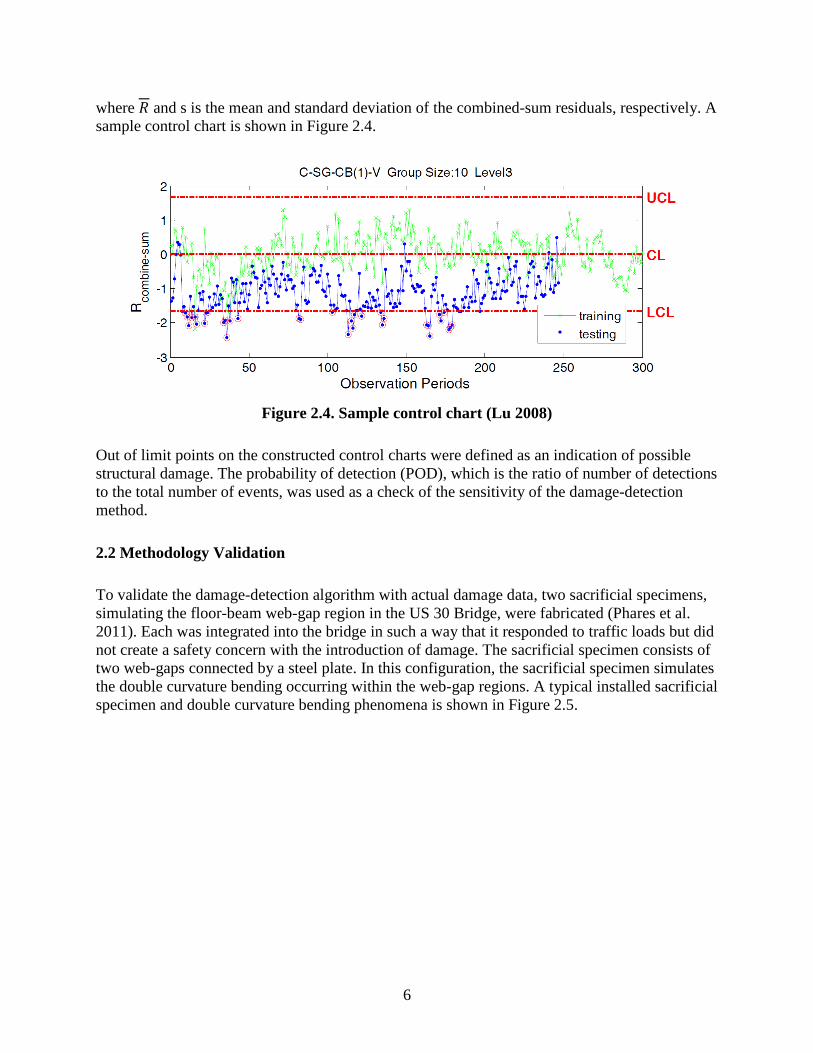
where and s is the mean and standard deviation of the combined-sum residuals, respectively. A

sample control chart is shown in Figure 2.4.

Figure 2.4. Sample control chart (Lu 2008)

Out of limit points on the constructed control charts were defined as an indication of possible

structural damage. The probability of detection (POD), which is the ratio of number of detections

to the total number of events, was used as a check of the sensitivity of the damage-detection

method.

2.2 Methodology Validation

To validate the damage-detection algorithm with actual damage data, two sacrificial specimens,

simulating the floor-beam web-gap region in the US 30 Bridge, were fabricated (Phares et al.

2011). Each was integrated into the bridge in such a way that it responded to traffic loads but did

not create a safety concern with the introduction of damage. The sacrificial specimen consists of

two web-gaps connected by a steel plate. In this configuration, the sacrificial specimen simulates

the double curvature bending occurring within the web-gap regions. A typical installed sacrificial

specimen and double curvature bending phenomena is shown in Figure 2.5.

7

Figure 2.5. Typical installed sacrificial specimen and double curvature bending of

sacrificial specimen (Phares et al. 2011)

2.2.1 Sacrificial Specimen 1

Specimen 1 was fabricated with a small electrical discharge machining (EDM) notch through the

thickness of the top plate where a crack was expected when high strains and a large number of

cycles occurred. It was found that the truck live loading strains in the specimen (and the

corresponding real web gap) were insufficient to grow a crack in a reasonable time. Therefore,

Specimen 1 was artificially damaged by attaching a rotary shaker to the specimen and cycling

the specimen rapidly near its resonance frequency in the range of 60 Hz to 70 Hz. Figure 2.6 and

2.7 show cracking in the top (left) and bottom (right) plates of the sacrificial specimen and

information on the installed sensor array, respectively.

Figure 2.6. Sacrificial Specimen 1 cracking (Phares et al. 2011)

8

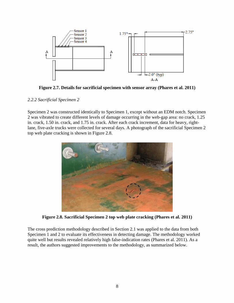
Figure 2.7. Details for sacrificial specimen with sensor array (Phares et al. 2011)

2.2.2 Sacrificial Specimen 2

Specimen 2 was constructed identically to Specimen 1, except without an EDM notch. Specimen

2 was vibrated to create different levels of damage occurring in the web-gap area: no crack, 1.25

in. crack, 1.50 in. crack, and 1.75 in. crack. After each crack increment, data for heavy, right-

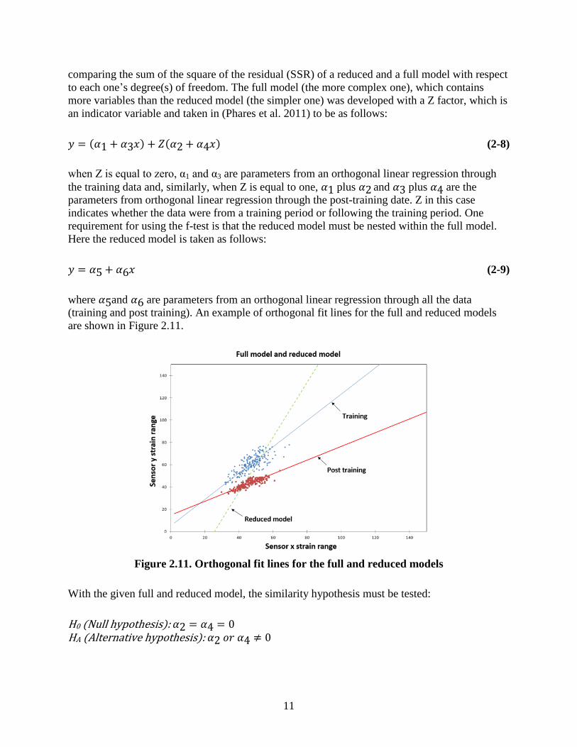
lane, five-axle trucks were collected for several days. A photograph of the sacrificial Specimen 2

top web plate cracking is shown in Figure 2.8.

Figure 2.8. Sacrificial Specimen 2 top web plate cracking (Phares et al. 2011)

The cross prediction methodology described in Section 2.1 was applied to the data from both

Specimen 1 and 2 to evaluate its effectiveness in detecting damage. The methodology worked

quite well but results revealed relatively high false-indication rates (Phares et al. 2011). As a

result, the authors suggested improvements to the methodology, as summarized below.

9

2.3 Orthogonal Regression and Statistical Evaluation Approach

Using orthogonal linear regression and the statistical f-test were proposed and developed to

reduce the relatively high false-detection rate associated with the previously-described cross

prediction damage-detection method. It was believed that these two methods would further

reduce uncertainties in the cross prediction methodology and, therefore, reduce the false-positive

rate.

2.3.1 Development of Orthogonal Regression and Orthogonal Residual

The most common use of orthogonal linear regression is in comparing two measurement systems

that both have measurement variations (Carroll and Ruppert 1996). In other words, the y

measurement variation and the x measurement variation are both the same. A standard linear

regression assumes that the x variable is fixed (i.e., no variation) and the y variable is a function

of x plus variation. Figure 2.9 shows samples of standard linear regression and orthogonal linear

regression.

Figure 2.9. Sample standard linear regression (left) and sample orthogonal linear

regression (right) (Phares et al. 2011)

The vertical bars in the chart on the left represent the y-residual and the negatively-sloping line

in the chart on the right represents the orthogonal residual. As with any linear regression, y and x

are related linearly through the following equation:

(2-3)

where b is the y-intercept and m is the slope.

The equation for standard linear regression can be developed by minimizing the sum of the

square of the y-residual, while the sum of the square of the perpendicular residual is minimized

in the orthogonal linear regression.

10

√ (2-4)

When the strain range data are in the first quadrant, an orthogonal residual is defined. An

example of an orthogonal line fit and an orthogonal residual is shown in Figure 2.10.

Figure 2.10. Example of an orthogonal line fit and an orthogonal residual

The sum of square of the perpendicular residuals (SSR) from the data points to the regression

line are given by the following:

∑

(2-5)

Minimizing SSR results in the following (Carroll and Ruppert 1996 and Fuller 1987):

{(

) }

(2-6)

(2-7)

where and

are the variance of the and data, respectively and is the covariance of

x and y that can be written in which is the correlation coefficient.

2.3.2 Damage Detection Approach with f-test

The f-test is typically used to evaluate the relationship between two different data sets

(Mendenhall and Sincich 2012). Generally, the purpose of the f-test is to quantify the amount of

model improvement achieved by including additional variables in the prediction model by

11

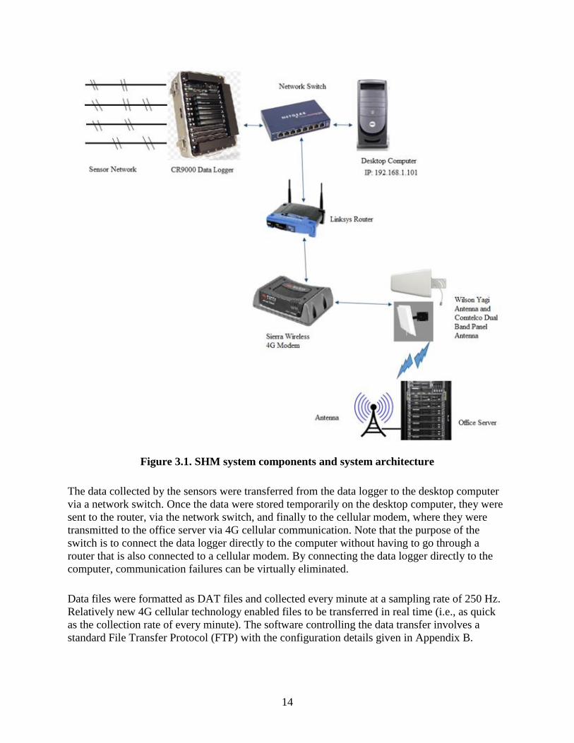
comparing the sum of the square of the residual (SSR) of a reduced and a full model with respect

to each one’s degree(s) of freedom. The full model (the more complex one), which contains

more variables than the reduced model (the simpler one) was developed with a Z factor, which is

an indicator variable and taken in (Phares et al. 2011) to be as follows:

( ) ( ) (2-8)

when Z is equal to zero, α1 and α3 are parameters from an orthogonal linear regression through

the training data and, similarly, when Z is equal to one, plus and plus are the

parameters from orthogonal linear regression through the post-training date. Z in this case

indicates whether the data were from a training period or following the training period. One

requirement for using the f-test is that the reduced model must be nested within the full model.

Here the reduced model is taken as follows:

(2-9)

where and are parameters from an orthogonal linear regression through all the data

(training and post training). An example of orthogonal fit lines for the full and reduced models

are shown in Figure 2.11.

Figure 2.11. Orthogonal fit lines for the full and reduced models

With the given full and reduced model, the similarity hypothesis must be tested:

H0 (Null hypothesis): HA (Alternative hypothesis):

12

If H0 is true, the reduced model is statistically the same as the full model as shown graphically in

Figure 2.12 (left) and it can be concluded that there is no damage at those two sensor locations.

On the other hand, if H0 is rejected, which is graphically illustrated in Figure 2.12, the reduced

model is significantly different from the full model and it may be an indication of damage.

Figure 2.12. Graphical representation of rejecting H0, no damage (left) and failing to reject

H0, damage (right)

To quantify these results, the f-test is conducted with the null hypothesis ( ) showing that the reduced model is able to fit the data set statistically as well as the full model. In

general, the F statistic is defined as follows (Caragea 2007):

(2-10)

where is the sum of the square of the residual of the reduced model and is the

sum of the square of the residual of the full model as given in Equation 2-5. df is the degrees of

freedom associated with an SSR; and are the degrees of freedom of the reduced

and full models, respectively. For the case of the models in Equation 2-11:

(2-11)

because the reduced model has two terms and the full model has four terms and n represents the

number of truck events, that is as follows. Note that is the sum of the squares of the

residuals for both training and post-training data.

(2-12)

(2-13)

(2-14)

13

3. DAMAGE DETECTION HARDWARE AND SOFTWARE

The fiber-optic sensing (FOS) SHM sensor system placed on the US 30 Bridge in 2006 and

briefly described in Chapter 2 was removed and replaced with updated hardware and software in

2012 as part of this project. The change in hardware from FOS to more traditional sensors was

determined to be a more cost-effective and robust approach. All software developed as part of

this project was developed specifically to interface with this hardware system. This chapter

presents the system configuration including the SHM hardware and network configuration, and it

also illustrates what a typical installation might consist of (using the US 30 Bridge as the case

study).

3.1 Hardware

3.1.1 Configuration

The SHM hardware at the US 30 Bridge installed for this work consists of electrical resistance

strain gauges that were run through completion bridge modules 4WF120 or 4WF350 depending

on the gauge resistance and hard-wired to a Campbell Scientific CR9000x data logger. The data

logger used the CR9052 module and programming was completed by using CRBasic language

from Campbell Scientific. The CR9052 cards were used specifically because they have the on-

board filtering needed when running high-speed acquisitions. This filtering helps in eliminating

electrical noise from the signal.

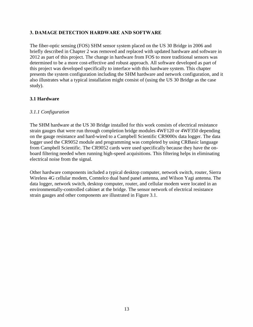
Other hardware components included a typical desktop computer, network switch, router, Sierra

Wireless 4G cellular modem, Comtelco dual band panel antenna, and Wilson Yagi antenna. The

data logger, network switch, desktop computer, router, and cellular modem were located in an

environmentally-controlled cabinet at the bridge. The sensor network of electrical resistance

strain gauges and other components are illustrated in Figure 3.1.

14

Figure 3.1. SHM system components and system architecture

The data collected by the sensors were transferred from the data logger to the desktop computer

via a network switch. Once the data were stored temporarily on the desktop computer, they were

sent to the router, via the network switch, and finally to the cellular modem, where they were

transmitted to the office server via 4G cellular communication. Note that the purpose of the

switch is to connect the data logger directly to the computer without having to go through a

router that is also connected to a cellular modem. By connecting the data logger directly to the

computer, communication failures can be virtually eliminated.

Data files were formatted as DAT files and collected every minute at a sampling rate of 250 Hz.

Relatively new 4G cellular technology enabled files to be transferred in real time (i.e., as quick

as the collection rate of every minute). The software controlling the data transfer involves a

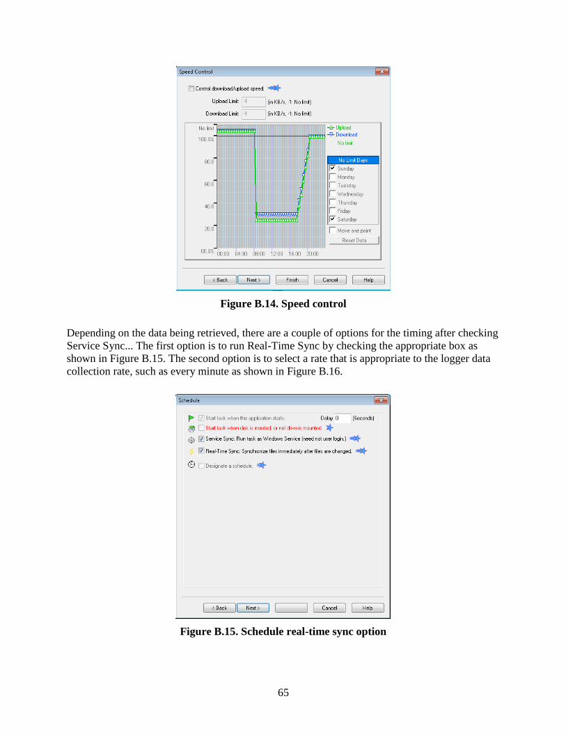
standard File Transfer Protocol (FTP) with the configuration details given in Appendix B.

15

3.1.2 Typical Installation

The first step in designing an SHM installation is to identify the goals associated with the

installation. Once the goals are identified, particular features of the bridge that are important for

achieving the goals can be identified. Finally, an instrumentation plan can be created to capture

data from these features.

The instrumentation plan for the US 30 Bridge deployed in this work consisted of 38 electrical

resistance strain gauges (120 and 350 ohm) and three thermocouples. An isometric view of the

US 30 Bridge and the cross sections of interest are shown in Figures 3.2 and 3.3, respectively.

Figure 3.2. Isometric view of US 30 Bridge

Figure 3.3. Bridge plan view for sensor layout

The strain gauge locations at each of the cross sections are shown in Figure 3.4.

16

a. Cross section X b. Cross section Y

c. Cross section C d. Cross section Z

Figure 3.4. Sensors locations within the bridge framing system

Sections X and Z are at mid-spans given that the maximum bending strains occur near these

locations. Section Y was chosen to be close to pier to quantify negative bending effects and

continuity behavior. Section C was chosen to capture the web-gap strains, which are of interest

because of the behavior in the web-gap cut-back region. Note that Section C is the same as

Section C in the FOS instrumentation system described previously. In addition, sensors were

placed strategically on the bottom of the deck as illustrated conceptually in Figure 3.5.

a. Deck bottom sensor line 1 b. Deck bottom sensor line 2

Figure 3.5. Sensor located on the bridge deck bottom

The specific locations of the deck sensors were chosen to identify vehicle travel lane, axle

number and spacing, and vehicle speed. Figure 3.6 shows a typical deck bottom sensor and a

girder top flange sensor.

17

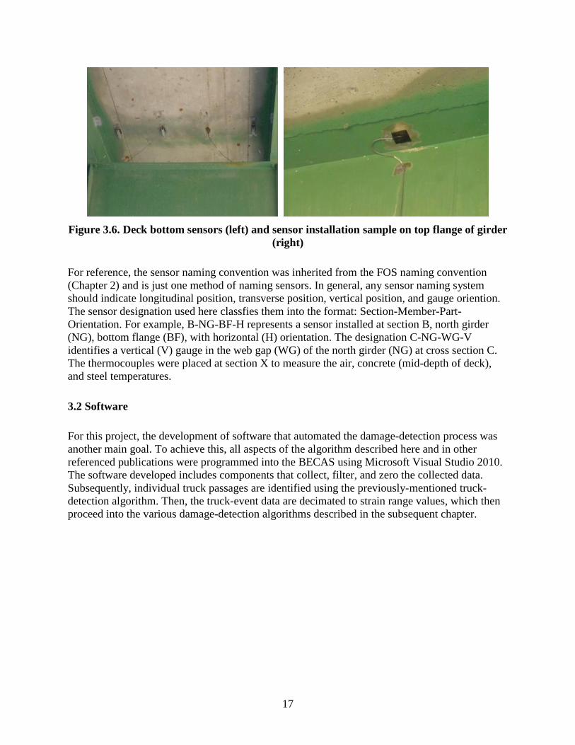
Figure 3.6. Deck bottom sensors (left) and sensor installation sample on top flange of girder

(right)

For reference, the sensor naming convention was inherited from the FOS naming convention

(Chapter 2) and is just one method of naming sensors. In general, any sensor naming system

should indicate longitudinal position, transverse position, vertical position, and gauge oriention.

The sensor designation used here classfies them into the format: Section-Member-Part-

Orientation. For example, B-NG-BF-H represents a sensor installed at section B, north girder

(NG), bottom flange (BF), with horizontal (H) orientation. The designation C-NG-WG-V

identifies a vertical (V) gauge in the web gap (WG) of the north girder (NG) at cross section C.

The thermocouples were placed at section X to measure the air, concrete (mid-depth of deck),

and steel temperatures.

3.2 Software

For this project, the development of software that automated the damage-detection process was

another main goal. To achieve this, all aspects of the algorithm described here and in other

referenced publications were programmed into the BECAS using Microsoft Visual Studio 2010.

The software developed includes components that collect, filter, and zero the collected data.

Subsequently, individual truck passages are identified using the previously-mentioned truck-

detection algorithm. Then, the truck-event data are decimated to strain range values, which then

proceed into the various damage-detection algorithms described in the subsequent chapter.

18

4. DAMAGE-DETECTION METHODOLOGIES

In this chapter, various enhancements to the previously-investigated damage-detection

methodologies using control charts are presented and investigated with actual data. The ability of

the methodologies to detect damage and the rate at which damage is identified falsely are

discussed.

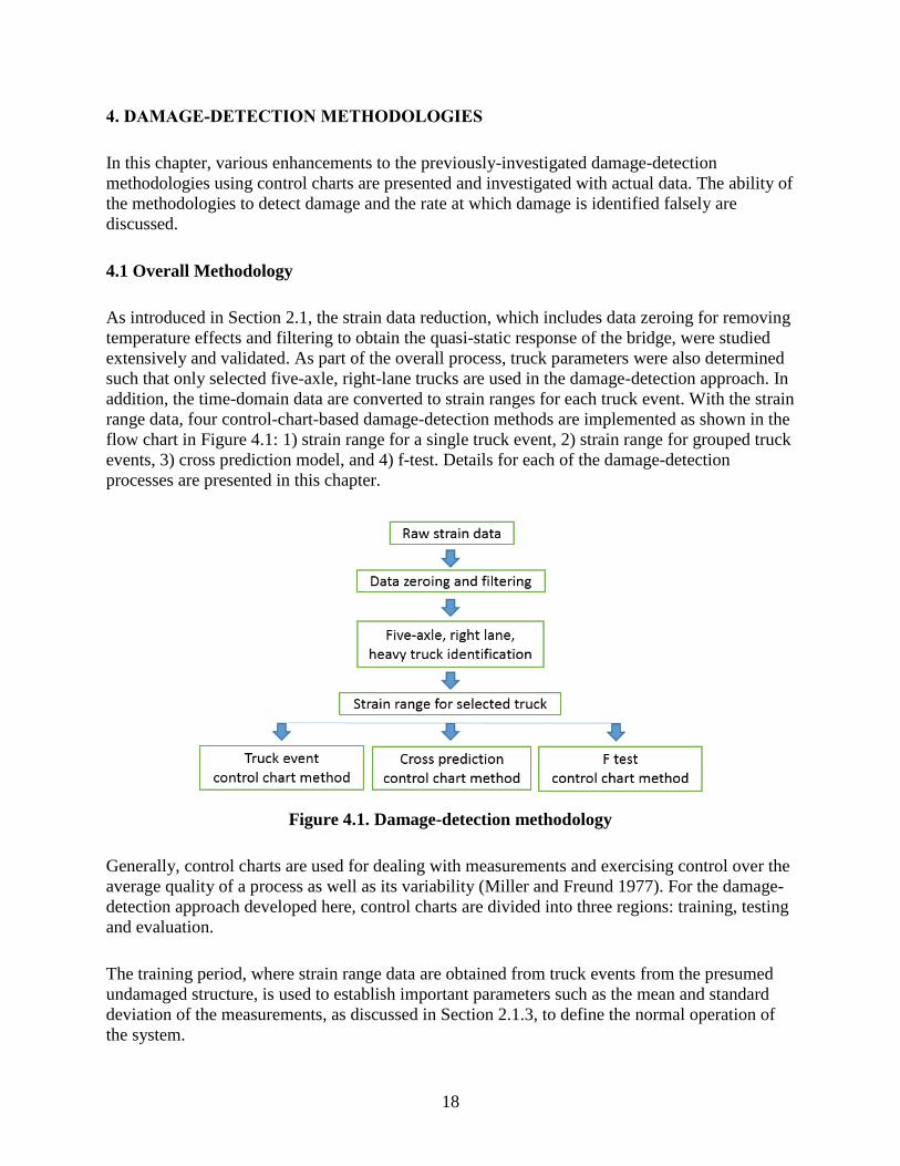
4.1 Overall Methodology

As introduced in Section 2.1, the strain data reduction, which includes data zeroing for removing

temperature effects and filtering to obtain the quasi-static response of the bridge, were studied

extensively and validated. As part of the overall process, truck parameters were also determined

such that only selected five-axle, right-lane trucks are used in the damage-detection approach. In

addition, the time-domain data are converted to strain ranges for each truck event. With the strain

range data, four control-chart-based damage-detection methods are implemented as shown in the

flow chart in Figure 4.1: 1) strain range for a single truck event, 2) strain range for grouped truck

events, 3) cross prediction model, and 4) f-test. Details for each of the damage-detection

processes are presented in this chapter.

Figure 4.1. Damage-detection methodology

Generally, control charts are used for dealing with measurements and exercising control over the

average quality of a process as well as its variability (Miller and Freund 1977). For the damage-

detection approach developed here, control charts are divided into three regions: training, testing

and evaluation.

The training period, where strain range data are obtained from truck events from the presumed

undamaged structure, is used to establish important parameters such as the mean and standard

deviation of the measurements, as discussed in Section 2.1.3, to define the normal operation of

the system.

19

Following the training period, a testing period is utilized to evaluate the efficacy of the training

period.

The evaluation period is for monitoring the bridge for change in structural performance (e.g.,

possible damage). In this chapter, evaluation data are further subdivided into the following

regions: Evaluation 1, Evaluation 2, Evaluation 3, and Evaluation 4.

For reference, the training period consisted of 2,000 truck events and the testing period consisted

of 1,000 truck events. The four evaluation periods represented times when there were varying

levels of damage present in the sacrificial Specimen 2. During Evaluation 1, no damage was

present. During Evaluation 2, a crack size of 1.25 in. was present. During Evaluation 3, a crack

size of 1.50 in. was present. During Evaluation 4, a crack size of 1.75 in. was present. When

implemented, the system will operate continuously during the evaluation period with

notifications of suspected damage sent in near real-time.

In the previous generation of the control-chart-based damage-detection methodologies, only a

single check was used to define when a change in structural behavior had occurred (when data

were greater than three standard deviations from the mean). Further investigation into process

control led to the realization that some process changes may be missed by only this single rule.

(Montogomery 1996) Therefore, additional rules were investigated, formulated, and evaluated.

Table 4.1 summarizes the six rules considered during methodology finalization and evaluation.

Table 4.1. Control chart rules (Montogomery 1996) and number of rule checks

Control chart rules

Number of

rule checks

#1 – One point beyond ±3s n

#2 – Two successive points out of three points beyond ±2s n-3

#3 – Four successive points out of five points ±1s n-5

#4 – Eight consecutive points on one side of the mean n-8

#5 – Six consecutive points trending up or down n-6

#6 – Fourteen consecutive points alternating up or down n-14

Each of these rules represents a different type of change in process control. In the context of

damage detection, the violation of any rule could be an indicator of a change in structural

condition.

From the perspective of a structural engineer, a false indication of damage occurs if one of the

control chart rules is violated but there is no damage (the incorrect rejection of a true null

hypothesis and sometimes called a type I error). For example, the circled points in Figure 4.2 are

false indications; that is, they are points outside the control limits but, for this particular case,

there is no known structural damage.

20

B-NG-BF-H

Figure 4.2. Example of false and true indication in a control chart

A true indication is defined as data points beyond the limits when there is truly damage. An

example of true indication, in the dashed ellipse (lower right of the chart), is shown in Figure 4.2.

After each specific damage-detection methodology is presented in this chapter, the methodology

will be applied to cases of no damage and actual damage and evaluated with respect to damage-

detection capability and with respect to false-indication rates.

4.2 Truck Event Control Chart Methods

4.2.1 Methodology

4.2.1.1 One-Truck Event Method

With the collected, filtered, and zeroed strain range data described in Section 4.1, control charts

can be constructed directly using the strain range for each truck event for each sensor without

further processing (i.e., one point on the control chart represents the strain range for a single

truck event). These control charts would therefore represent the response data in their most basic

form. In addition, in this form, a graphical representation is interpreted easily with fundamental

structural engineering concepts. Control charts and associated limits are constructed using the

mean and standard deviation of all trucks in the training period.

4.2.1.2 Truck Events Grouped by Ten Method

Group size can be an important parameter in constructing a control chart because it affects the

control limits and the sensitivity of the false-indication rate. For example, the larger the group

size, the narrower the control limits; therefore, slight damage could be detected from small

variations (Lu et al. 2010). However, at the same time, larger group sizes increase the time that it

takes for damage to be identified.

21

The optimal group size was previously determined to be 10 for this work (Lu 2008). Similar to

the one-truck event approach, the mean of the means and standard deviations from data for 10

trucks (one group) are used as the chart variables. As before, the mean and standard deviations of

the grouped strain range data during the training period are used to construct the control charts.

4.2.2 Select Results

The sensors listed in Table 4.2 will be used to illustrate the application of the truck event control

chart methods for one-truck event (Section 4.2.1.1) and truck events grouped by ten (Section

4.2.1.2) below. These sensors were selected because they are typical of all results and they

represent diverse sensor locations that include sensors on the bridge and on the sacrificial

specimen.

Table 4.2. List of select sensors used to create sample control charts

Sensor Name

B-NG-BF-H

B-SG-BF-H

C-SG-BF-H

C-SG-CB(5)-V

C-SG-CB(4)-V

C-NG-BF-H

Sensor 1 on sacrificial specimen

Sensor 4 on sacrificial specimen

4.2.2.1 One-Truck Event Control Chart

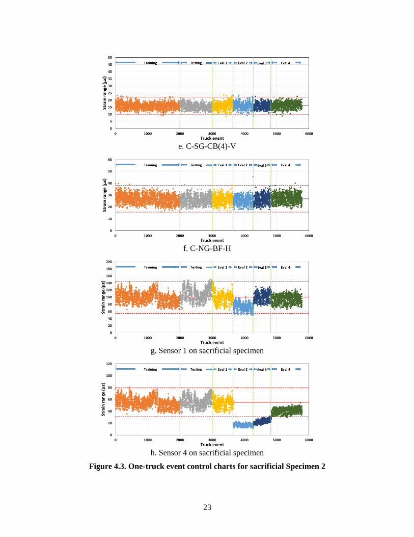
Examples of one-truck event control charts for Specimen 2 for the selected sensors are shown in

Figure 4.3. To establish the control limits for the various rules described in Section 4.1, the mean

and standard deviation were calculated to be as shown in Table 4.3.

Table 4.3. Mean and standard deviations of select sensors for one-truck event method

Sensor name Mean

Standard

deviation

B-NG-BF-H 44 6

B-SG-BF-H 103 12

C-SG-BF-H 32 4

C-SG-CB(5)-V 92 11

C-SG-CB(4)-V 16 2

C-NG-BF-H 27 4

Sensor 1 on sacrificial specimen 100 15

Sensor 4 on sacrificial specimen 55 8

22

a. B-NG-BF-H

b. B-SG-BF-H

c. C-SG-BF-H

d. C-SG-CB(5)-V

23

e. C-SG-CB(4)-V

f. C-NG-BF-H

g. Sensor 1 on sacrificial specimen

h. Sensor 4 on sacrificial specimen

Figure 4.3. One-truck event control charts for sacrificial Specimen 2

24

To summarize the propensity for violating the rules in Table 4.1, a table was developed to

summarize the number of times that each rule was violated during each monitoring period. The

rule violations for the one-truck event control chart method for select sensor are summarized in

Table 4.4 and an additional table for all sensors is shown in Appendix A.

Table 4.4. Rule violations for one-truck event method

Sensor Period Rule 1 Rule 2 Rule 3 Rule 4 Rule 5 Rule 6 Total

B-NG-BF-H Training 9 15 93 148 7 15 287

Testing 2 2 42 82 5 7 140

Evaluation 1 2 15 44 1 62

Evaluation 2 1 4 35 62 2 1 105

Evaluation 3 2 3 19 42 1 1 68

Evaluation 4 5 6 22 45 3 2 83

Total 21 30 226 423 19 26 745

Rate (%) 0.4 0.5 3.9 7.3 0.3 0.5 2.1

B-SG-BF-H Training 1 2 147 239 5 8 402

Testing 88 172 2 5 267

Evaluation 1 5 52 62 2 9 130

Evaluation 2 2 88 133 4 227

Evaluation 3 41 87 1 129

Evaluation 4 40 79 5 5 129

Total 1 9 456 772 19 27 1284

Rate (%) 0.2 0.2 7.9 13.4 0.3 0.5 3.7

C-SG-BF-H Training 1 17 123 138 5 11 295

Testing 1 6 90 143 5 1 246

Evaluation 1 1 3 38 78 6 126

Evaluation 2 1 7 50 133 4 195

Evaluation 3 1 9 56 40 6 3 115

Evaluation 4 3 68 58 1 130

Total 8 42 425 590 21 21 1107

Rate (%) 0.1 0.7 7.4 10.2 0.4 0.4 3.2

C-SG-CB(5)-V Training 2 15 76 129 2 16 240

Testing 5 70 103 2 2 182

Evaluation 1 2 8 18 47 7 82

Evaluation 2 1 3 34 72 2 3 115

Evaluation 3 1 4 42 43 1 91

Evaluation 4 8 37 120 198 2 1 366

Total 14 72 360 592 9 29 1076

Rate (%) 0.2 1.2 6.2 10.3 0.2 0.5 3.10

25

Sensor Period Rule 1 Rule 2 Rule 3 Rule 4 Rule 5 Rule 6 Total

C-SG-CB(4)-V Training 11 33 108 141 8 18 319

Testing 12 77 189 2 280

Evaluation 1 8 37 55 60 7 167

Evaluation 2 9 33 96 111 9 258

Evaluation 3 1 4 19 53 1 1 79

Evaluation 4 4 4 50 89 1 2 150

Total 33 123 405 643 28 21 1253

Rate (%) 0.6 2.1 7.0 11.1 0.5 0.4 3.62

C-NG-BF-H Training 4 18 137 242 9 3 413

Testing 1 1 68 123 1 6 200

Evaluation 1 1 39 47 1 88

Evaluation 2 1 8 48 88 1 146

Evaluation 3 37 69 3 3 112

Evaluation 4 2 1 26 64 1 94

Total 9 28 355 633 16 12 1053

Rate (%) 0.2 0.5 6.2 11.0 0.3 0.2 3.0

Sensor 1 on

sacrificial

specimen

Training 46 311 451 8 8 824

Testing 17 129 289 322 3 4 764

Evaluation 1 23 100 161 2 4 290

Evaluation 2 30 174 467 608 1 1280

Evaluation 3 24 73 1 3 101

Evaluation 4 1 43 103 1 1 149

Total 47 373 1234 1718 16 20 3408

Rate (%) 0.8 6.5 21.4 29.8 0.3 0.4 9.8

Sensor 4 on

sacrificial

specimen

Training 1 38 300 440 8 8 795

Testing 25 207 193 4 1 430

Evaluation 1 2 54 104 1 4 165

Evaluation 2 627 625 623 620 2495

Evaluation 3 549 549 547 544 1 3 2193

Evaluation 4 1 181 821 945 3 8 1959

Total 1178 1420 2552 2846 17 24 8037

Rate (%) 20.4 24.6 44.2 49.3 0.3 0.4 23.2

Figure 4.3 and Table 4.4 show that during the training, testing, and Evaluation 1 periods (when

there was no damage), there were a number of rule violations and the majority of those violations

resulted from either Rule 3 or Rule 4. The rule violation rate for all sensors on the bridge were

similar during all phases of monitoring indicating that the system was operating in a stable

manner (also observable in Table 4.5). Once damage was introduced, the sensors on the

specimen were collectively able to identify the damage with multiple rule violations of multiple

types.

For each control chart region and each sensor, the number of rule violations and rate with respect

to the six rules are counted and calculated by the automated software, BECAS, and are

summarized in Table 4.4. The relatively high number of rule violations from Rule 3 and 4

26

significantly affect the overall false-indication rate. Table 4.5 shows the number of false

indications for sensors on the bridge (non-damaged).

Table 4.5. Number of false indications for sensors on bridge (non-damaged) for one-truck

event method

Sensor with

no damage

False indications

(Training, Testing,

Evaluation

1, 2, 3, and 4)

False

indication

rate

(%)

B-NG-BF-H 745 2.2

B-SG-BF-H 1284 3.7

C-SG-BF-H 1107 3.2

C-SG-CB(5)-V 1076 3.1

C-SG-CB(4)-V 1253 3.6

C-NG-BF-H 1053 3.0

When there was real damage near the sensors on the sacrificial specimen, the true-indication rate

can be investigated by considering the Evaluation 2, 3, and 4 regions, which are summarized in

Table 4.6. Note that, as expected, the true-indication rate is higher for Sensor 4 placed near the

crack than for Sensor 1 placed away from the crack.

Table 4.6. Number of false and true indications for sensors on sacrificial specimen (near

damage) for one-truck event method

Sensor

near

damage

False

indications

(Training, Testing,

Evaluation 1)

False

indication

rate

(%)

True

indications

(Evaluation

2, 3, and 4)

True

indication

rate

(%)

Sensor 1 1878 8.6 1530 12.0

Sensor 4 1390 6.4 6647 52.2

4.2.2.2 Truck Events Grouped by Ten Control Chart

Examples of truck events grouped by ten control charts for Specimen 2 for select sensors are

shown in Figure 4.4. The mean and standard deviation were calculated to establish the control

limits for the various rules and are shown in Table 4.7. Note that the mean values are

approximately the same as the one-truck event method but that the standard deviation is notably

narrower because of the grouping process.

27

a. B-NG-BF-H

b. B-SG-BF-H

c. C-SG-BF-H

d. C-SG-CB(5)-V

28

e. C-SG-CB(4)-V

f. C-NG-BF-H

g. Sensor 1 on sacrificial specimen

h. Sensor 4 on sacrificial specimen

Figure 4.4. Truck events grouped by ten control charts for sacrificial Specimen 2

29

Table 4.7. Mean and standard deviations of select sensors (µε) for truck events grouped by

ten method

Sensor name Mean

Standard

deviation

B-NG-BF-H 44 3

B-SG-BF-H 103 7

C-SG-BF-H 32 2

C-SG-CB(5)-V 92 6

C-SG-CB(4)-V 16 1

C-NG-BF-H 27 2

Sensor 1 on

sacrificial specimen

100 11

Sensor 4 on

sacrificial specimen

56 6

As with the one-truck event methodology, a table was constructed to summarize the tendency for

violating the control chart rules. From Figure 4.4 and Table 4.8, it is observed that during the

training, testing, and Evaluation 1 periods (when there was no damage), there were a number of

rule violations and that the majority of those resulted from either Rule 3 or Rule 4.

From Figure 4.4, sensors on the bridge (non-damaged) follow control chart Rule 1 well. It was

also found that sensors near damage (i.e., Sensor 4) show violations of Rule 1 in the Evaluation

2, 3, and 4 regions. In Table 4.8, the methodology found significantly high numbers of rule

violations from Rule 3 and Rule 4 and those violations affect the overall false-indication rate

significantly.

Table 4.8. Rule violations for truck events grouped by ten method

Sensor Period Rule 1 Rule 2 Rule 3 Rule 4 Rule 5 Rule 6 Total

B-NG-BF-H Training 1 1 21 18 4

45

Testing

12 10 3

25

Evaluation 1

9 3 2

14

Evaluation 2

2 6 1

9

Evaluation 3

6 6

12

Evaluation 4

6 13

19

Total 1 3 60 51 9 0 124

Rate (%) 0.2 0.5 10.5 9.0 1.6 0 3.61

B-SG-BF-H Training

6 36 7 4

53

Testing

3 22 5 11

41

Evaluation 1 1 2 12 6 2

23

Evaluation 2

6 17 3 3

29

Evaluation 3

2 14

3

19

Evaluation 4

9

9

Total 1 19 110 21 23 0 174

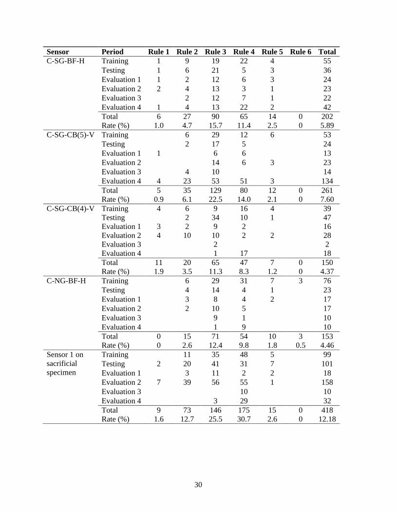
Rate (%) 0.2 3.3 19.2 3.7 4.0 0 5.07

30

Sensor Period Rule 1 Rule 2 Rule 3 Rule 4 Rule 5 Rule 6 Total

C-SG-BF-H Training 1 9 19 22 4

55

Testing 1 6 21 5 3

36

Evaluation 1 1 2 12 6 3

24

Evaluation 2 2 4 13 3 1

23

Evaluation 3

2 12 7 1

22

Evaluation 4 1 4 13 22 2

42

Total 6 27 90 65 14 0 202

Rate (%) 1.0 4.7 15.7 11.4 2.5 0 5.89

C-SG-CB(5)-V

Training

6 29 12 6

53

Testing

2 17 5

24

Evaluation 1 1

6 6

13

Evaluation 2

14 6 3

23

Evaluation 3

4 10

14

Evaluation 4 4 23 53 51 3

134

Total 5 35 129 80 12 0 261

Rate (%) 0.9 6.1 22.5 14.0 2.1 0 7.60

C-SG-CB(4)-V Training 4 6 9 16 4

39

Testing

2 34 10 1

47

Evaluation 1 3 2 9 2

16

Evaluation 2 4 10 10 2 2

28

Evaluation 3

2

2

Evaluation 4

1 17

18

Total 11 20 65 47 7 0 150

Rate (%) 1.9 3.5 11.3 8.3 1.2 0 4.37

C-NG-BF-H Training

6 29 31 7 3 76

Testing

4 14 4 1

23

Evaluation 1

3 8 4 2

17

Evaluation 2

2 10 5

17

Evaluation 3

9 1

10

Evaluation 4

1 9

10

Total 0 15 71 54 10 3 153

Rate (%) 0 2.6 12.4 9.8 1.8 0.5 4.46

Sensor 1 on

sacrificial

specimen

Training

11 35 48 5

99

Testing 2 20 41 31 7

101

Evaluation 1

3 11 2 2

18

Evaluation 2 7 39 56 55 1

158

Evaluation 3

10

10

Evaluation 4

3 29

32

Total 9 73 146 175 15 0 418

Rate (%) 1.6 12.7 25.5 30.7 2.6 0 12.18

31

Sensor Period Rule 1 Rule 2 Rule 3 Rule 4 Rule 5 Rule 6 Total

Sensor 4 on

sacrificial

specimen

Training

10 30 67 5

112

Testing

2 33 33 7

75

Evaluation 1

9 2 1

12

Evaluation 2 62 60 58 55 2

237

Evaluation 3 55 53 51 48

207

Evaluation 4 2 72 91 88

253

Total 119 197 272 293 15 0 896

Rate (%) 20.6 34.3 47.5 51.4 2.6 0 26.1

Tables 4.9 and 4.10 summarize the number of false indications for sensors on the bridge (non-

damaged) and the number of false and true indications for sensors on the specimen (near

damage). It was found that the true-indication rate is similar to the one-truck event method.

Table 4.9. Number of false indications for sensors on bridge (non-damaged) for truck

events grouped by ten method

Sensor with

no damage

False indications

(Training, Testing,

Evaluation

1, 2, 3, and 4)

False

indication

rate

(%)

B-NG-BF-H 124 3.6

B-SG-BF-H 174 5.1

C-SG-BF-H 202 5.9

C-SG-CB(5)-V 261 7.9

C-SG-CB(4)-V 150 4.4

C-NG-BF-H 153 4.5

Table 4.10. Number of false and true indications for sensors on sacrificial specimen (near

damage) for truck events grouped by ten method

Sensor

near

damage

False

indications

(Training, Testing,

Evaluation 1)

False

indication

rate

(%)

True

indications

(Evaluation

2, 3, and 4)

True

indication

rate

(%)

Sensor 1 218 10.4 200 16.1

Sensor 4 199 9.2 697 56.1

4.3 Cross Prediction Control Chart Method

4.3.1 Methodology

Fundamentally, the cross prediction method presented here is an adaptation of the method

described in Chapter 2. The primary differences in the methodology are the use of orthogonal

32

regression and the simplification approach. Like the method presented in Chapter 2, truck events

are grouped into a group size of 10. A general flow chart for the method is shown in Figure 4.5.

Figure 4.5. Cross prediction method flow chart

During training, orthogonal regression as described in Section 2.3.1 is performed for every

combination of sensor pairs, εi and εj, where i and j range from 1 to q (number of sensors).

Because orthogonal regression is used, the relationship between εi and εj is the inverse of the

relationship between εj and εi. Orthogonal residuals are then calculated as previously discussed in

Section 2.3.1 and assembled into residual matrixes (q by q) for each truck group with p (number

of groups) of these matrices.

[ ] [

] (4-1)

33

Standardizing the residuals are helpful to normalize the residual values that vary over a large

range of values (Lu 2008). The process for standardizing the residual for all sensor pairs for each

truck group is given in Equations 4-2 and 4-3:

(4-2)

[ ] [

] [ ] [

] (4-3)

where is the average of for all the groups and is the standard deviation. This process

results in another set of q by q standardized-residual matrices and there are p of these, with one

for each group.

[ ] [

] (4-4)

To further simply the standardized-residual data to a single control chart for each sensor, the

standardized residual matrix [ ] is reduced to a set of p simplified residual vectors [ ] by

summing each row.

∑ (4-5)

[ ]

[ ]

(4-6)

The mean and standard deviation of the [ ] residuals for all training truck groups are calculated

and then used to set control limits.

[ ]

[

]

[ ]

[ ]

(4-7)

For each group of 10 truck events occurring during subsequent monitoring, an orthogonal

residual matrix is obtained by using the orthogonal regression from the training period (Equation

4-1). The mean and standard deviation of the standardized residual (Equation 4-2) from the

34

training period are again used to calculate the standardized residuals (Equation 4-4) and, after the

residual-simplification process, a point Ri for this group is plotted on each control chart.

4.3.2 Select Results

With the cross prediction method, the average of the standardized residuals are always equal to

zero due to the standardization process. As was mentioned previously, the standard deviations

are used to establish control limits that are applied to the various rules. Table 4.11 shows the

mean and standard deviations of select sensors. As can be seen in Table 4.11, there was a fair

amount of consistency in the standard deviations indicating that the standardization process was

effective at reducing large ranges of residual values.

Table 4.11. Mean and standard deviations of selected sensors (µε) for cross prediction

method

Sensor name Mean

Standard

deviation

B-NG-BF-H 0 25

B-SG-BF-H 0 21

C-SG-BF-H 0 29

C-SG-CB(5)-V 0 19

C-SG-CB(4)-V 0 34

C-NG-BF-H 0 28

Sensor 1 on sacrificial specimen 0 26

Sensor 4 on sacrificial specimen 0 25

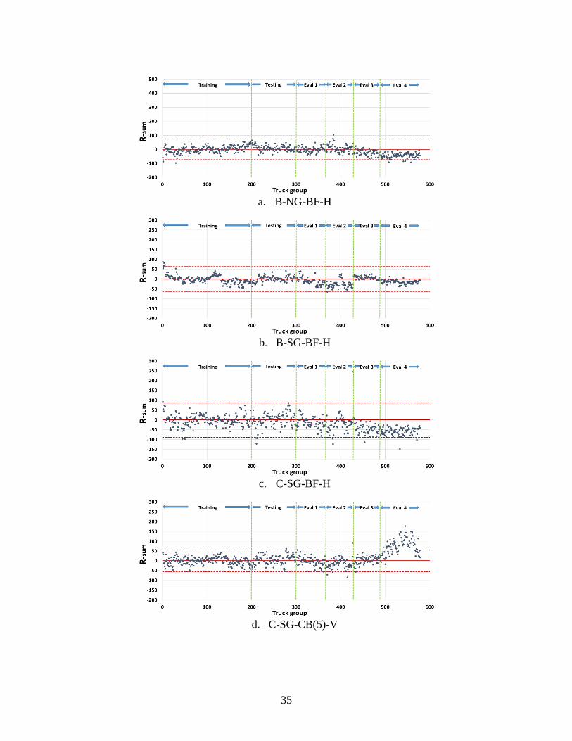
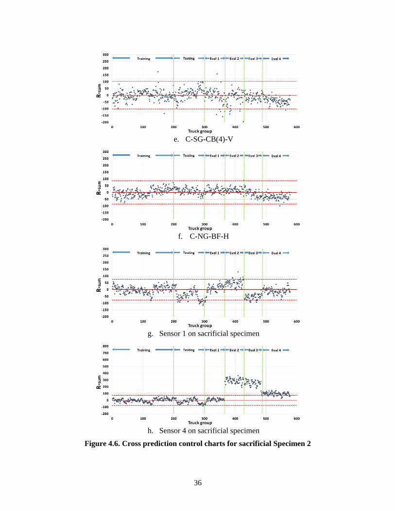
In Figure 4.6, R-sum values for global response sensors on the bridge (non-damaged) follow

Rule 1 well, as data points are generally within the plus/minus three standard deviation limits.

However, there are a large number of false indications (Rule 1) for sensors placed in the web cut-

back region of the bridge (Sensors C-SG-CB(5)-V and C-SG-CB(4)-V). In Figure 4.6h, for

example, it would be inferred that there is damage because the R-sum values exceed the limits

for Rule 1 in the Evaluation 2, 3, and 4 regions.

The number of rule violations and rate with respect to all rules were determined and are shown in

Table 4.12. A large number of rule violations are found for Rule 3 or Rule 4 as was the case with

the strain range methods.

35

a. B-NG-BF-H

b. B-SG-BF-H

c. C-SG-BF-H

d. C-SG-CB(5)-V

36

e. C-SG-CB(4)-V

f. C-NG-BF-H

g. Sensor 1 on sacrificial specimen

h. Sensor 4 on sacrificial specimen

Figure 4.6. Cross prediction control charts for sacrificial Specimen 2

37

Table 4.12. Rule violations for cross prediction method

Sensor Period Rule 1 Rule 2 Rule 3 Rule 4 Rule 5 Rule 6 Total

B-NG-BF-H Training 2 3 14 31 2 52

Testing 8 11 1 20

Evaluation 1 2 2

Evaluation 2 2 4 5 3 14

Evaluation 3 4 22 26

Evaluation 4 4 24 70 88 186

Total 8 31 103 155 3 0 300

Rate (%) 1.4 5.4 18.0 27.2 0.5 0.0 8.7

B-SG-BF-H Training 5 6 21 87 5 124

Testing 5 13 5 23

Evaluation 1 10 29 39

Evaluation 2 1 10 36 42 89

Evaluation 3 6 6

Evaluation 4 7 69 76

Total 6 16 79 246 10 0 357

Rate (%) 1.0 2.8 13.8 43.2 1.8 0.0 10.4

C-SG-BF-H Training 3 6 22 13 2 46

Testing 3 8 11 6 4 32

Evaluation 1 2 3 6 2 13

Evaluation 2 3 10 20 24 3 60

Evaluation 3 1 14 37 45 1 98

Evaluation 4 5 41 85 88 219

Total 15 81 178 182 12 0 468

Rate (%) 2.6 14.1 31.1 31.9 2.1 0.0 13.6

C-SG-CB(5)-V

Training 1 12 11 24

Testing 1 12 19 17 2 51

Evaluation 1 2 4 1 1 8

Evaluation 2 4 3 17 11 35

Evaluation 3 1 2 3

Evaluation 4 59 76 77 72 2 286

Total 65 96 129 112 5 0 407

Rate (%) 11.3 16.7 22.5 19.7 0.9 0.0 11.9

C-SG-CB(4)-V Training 2 2 5 27 1 37

Testing 10 25 20 2 57

Evaluation 1 5 4 2 5 16

Evaluation 2 8 10 12 5 1 36

Evaluation 3 2 5 7

Evaluation 4 1 4 34 55 1 95

Total 16 30 80 117 5 0 248

Rate (%) 2.8 5.2 14.0 20.5 0.9 0.00 7.2

38

Sensor Period Rule 1 Rule 2 Rule 3 Rule 4 Rule 5 Rule 6 Total

C-NG-BF-H Training 6 16 41 1 64

Testing 11 18 1 30

Evaluation 1 9 16 1 26

Evaluation 2 1 12 1 14

Evaluation 3 7 4 11

Evaluation 4 1 2 37 58 98

Total 2 8 80 149 4 0 243

Rate (%) 0.4 1.4 14.0 26.1 0.7 0.0 7.08

Sensor 1 on

sacrificial

specimen

Training 2 6 21 32 1 1 63

Testing 25 47 59 58 1 190

Evaluation 1 3 6 15 23 5 52

Evaluation 2 7 30 42 39 118

Evaluation 3 9 31 50 48 2 140

Evaluation 4 3 16 6 25

Total 46 123 203 206 9 1 588

Rate (%) 8.0 21.4 35.4 36.1 1.6 0.2 17.1

Sensor 4 on

sacrificial

specimen

Training 6 31 47 6 1 91

Testing 2 23 43 35 2 105

Evaluation 1 3 5 12 2 22

Evaluation 2 63 61 59 55 1 239

Evaluation 3 55 53 51 48 207

Evaluation 4 79 89 91 88 347

Total 199 235 280 285 11 1 1011

Rate (%) 34.4 40.9 48.9 50.0 1.9 0.2 29.5

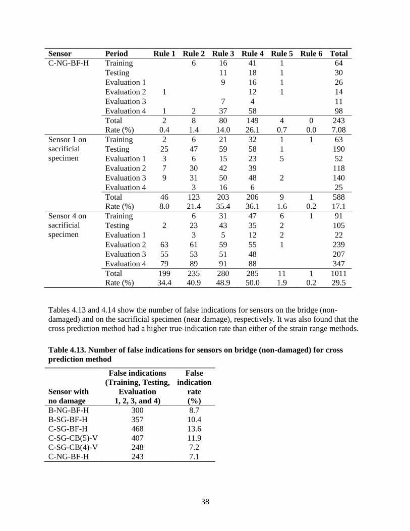
Tables 4.13 and 4.14 show the number of false indications for sensors on the bridge (non-

damaged) and on the sacrificial specimen (near damage), respectively. It was also found that the

cross prediction method had a higher true-indication rate than either of the strain range methods.

Table 4.13. Number of false indications for sensors on bridge (non-damaged) for cross

prediction method

Sensor with

no damage

False indications

(Training, Testing,

Evaluation

1, 2, 3, and 4)

False

indication

rate

(%)

B-NG-BF-H 300 8.7

B-SG-BF-H 357 10.4

C-SG-BF-H 468 13.6

C-SG-CB(5)-V 407 11.9

C-SG-CB(4)-V 248 7.2

C-NG-BF-H 243 7.1

39

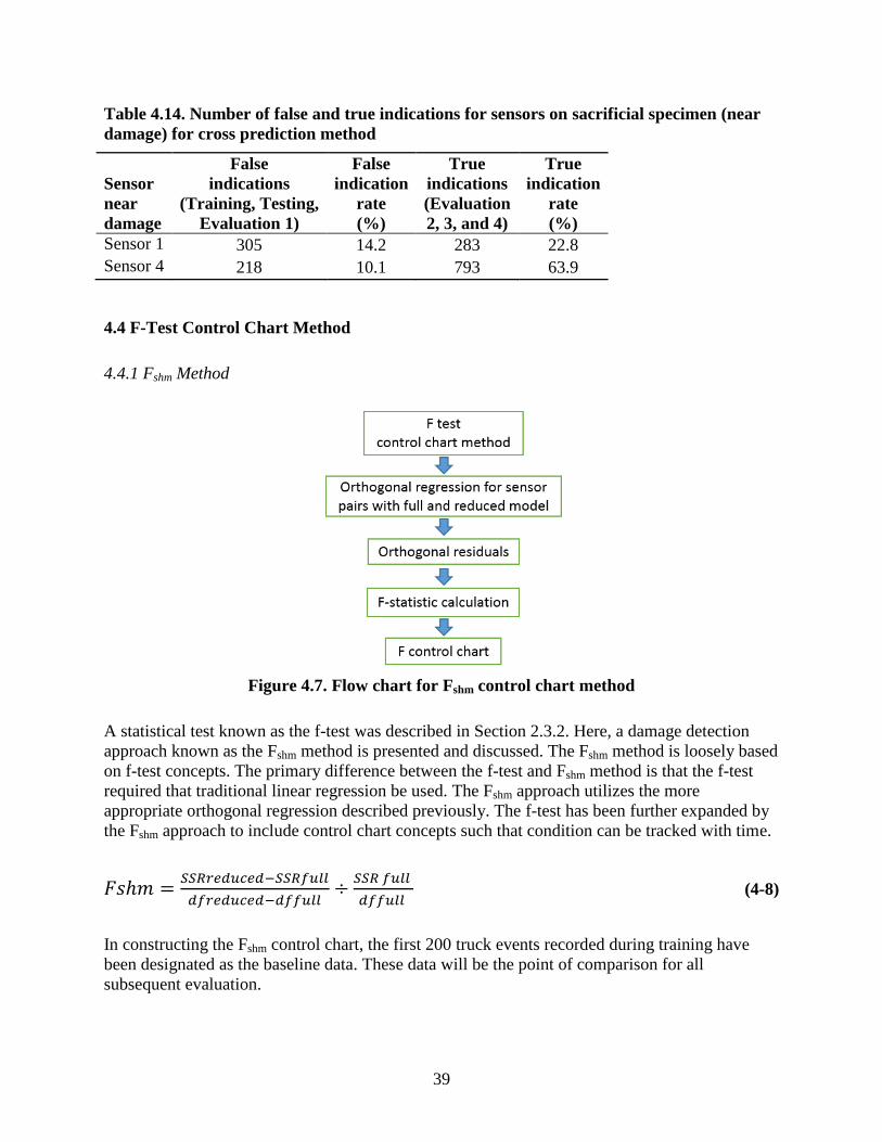
Table 4.14. Number of false and true indications for sensors on sacrificial specimen (near

damage) for cross prediction method

Sensor

near

damage

False

indications

(Training, Testing,

Evaluation 1)

False

indication

rate

(%)

True

indications

(Evaluation

2, 3, and 4)

True

indication

rate

(%)

Sensor 1 305 14.2 283 22.8

Sensor 4 218 10.1 793 63.9

4.4 F-Test Control Chart Method

4.4.1 Fshm Method

Figure 4.7. Flow chart for Fshm control chart method

A statistical test known as the f-test was described in Section 2.3.2. Here, a damage detection

approach known as the Fshm method is presented and discussed. The Fshm method is loosely based

on f-test concepts. The primary difference between the f-test and Fshm method is that the f-test

required that traditional linear regression be used. The Fshm approach utilizes the more

appropriate orthogonal regression described previously. The f-test has been further expanded by

the Fshm approach to include control chart concepts such that condition can be tracked with time.

(4-8)

In constructing the Fshm control chart, the first 200 truck events recorded during training have

been designated as the baseline data. These data will be the point of comparison for all

subsequent evaluation.

40

For trucks from 201 through 2,000, groups of 200 trucks (with 150 trucks overlapping between

groups) are compared against the baseline data using the Fshm equation. This ensures that all Fshm

values have the same sample size (200 are from the baseline data and another 200 are for

comparison). Collectively, this series of Fshm values are then used to establish the mean and

standard deviations for all such evaluations made during the training period (up through truck

number 2,000). The means and standard deviations then establish the control chart limits by

which the various tests will be evaluated.

With this approach, the data are evaluated via sensor pairings, much like the early portion of the

cross prediction methodology. However, unlike the cross prediction method, no simplification is

made and, therefore, (n2-n)/2 evaluations are made. This results in a very large number of

evaluations being made after each successive passage of 50 trucks.

4.4.2 Select Results

To study the Fshm approach, 12 sensor pairs were selected and the mean and standard deviation

from the training period were calculated (listed in Table 4.15) as described in the previous

section. As expected, high Fshm values resulted for sensor pairs that included a sensor on the

sacrificial specimen during the Evaluation 2, 3, and 4 periods indicating that damage was readily

detected.

Table 4.15. Mean and standard deviations of select sensors (µε) for Fshm method

Sensor pairs Mean

Standard

deviation

B-NG-BF-H vs. B-SG-BF-H 18 13

B-NG-BF-H vs. C-SG-BF-H 4 3

B-NG-BF-H vs. C-SG-CB(5)-V 6 6

B-NG-BF-H vs. C-SG-CB(4)-V 6 6

B-SG-BF-H vs. C-NG-BF-H 30 27

C-SG-BF-H vs. C-NG-BF-H 17 12

C-SG-CB(5)-V vs. C-SG-CB(4)-V 8 11

C-SG-CB(5)-V vs. C-NG-BF-H 9 11

C-SG-CB(4)-V vs. C-NG-BF-H 9 9

B-NG-BF-H vs. Sensor 4 23 14

B-SG-BF-H vs. Sensor 1 89 84

B-SG-BF-H vs. Sensor 4 149 136

As Table 4.16 shows, no rule violations were found for Rules 6 or 3 and Rule 4 had many rule

violations as was observed for the other methodologies.

41

Table 4.16. Rule violations for Fshm control chart

Sensor pairs Period Rule 1 Rule 2 Rule 3 Rule 4 Rule 5 Rule 6 Total

B-NG-BF-H

vs.

B-SG-BF-H

Training 2 9 14 4 29

Testing 2 2 1 5 2 12

Evaluation 1 1 1 5 1 8

Evaluation 2 2 7 3 8 20

Evaluation 3 4 4 6 14

Evaluation 4 11 19 30

Total 4 12 29 55 13 0 113

Rate (%) 3.7 11.4 28.2 55.0 12.8 0.0 18.5

B-NG-BF-H

vs.

C-SG-BF-H

Training 3 1 2 6

Testing 4 4 2 2 2 14

Evaluation 1 2 4 6 1 1 14

Evaluation 2 6 8 3 6 23

Evaluation 3 4 8 9 7 28

Evaluation 4 2 3 4 19 28

Total 18 27 27 36 5 0 113

Rate (%) 16.7 25.7 26.2 36.0 4.9 0.0 18.5

B-NG-BF-H

vs.

C-SG-CB(5)-H

Training 1 2 5 13 1 22

Testing 3 2 1 5 2 13

Evaluation 1 1 2 1 3 7

Evaluation 2 3 7 5 3 2 20

Evaluation 3 1 2 3

Evaluation 4 1 4 12 2 19

Total 7 13 17 35 12 0 84

Rate (%) 6.5 12.4 16.5 35.0 11.8 0.0 13.7

B-NG-BF-H

vs.

C-SG-CB(4)-V

Training 6 7 23 36

Testing 2 2 2 11 1 18

Evaluation 1 1 1

Evaluation 2 11 11

Evaluation 3 0

Evaluation 4 10 10

Total 2 2 9 39 24 0 76

Rate (%) 1.9 1.9 8.7 39.0 23.5 0.0 12.4

B-SG-BF-H

vs.

C-NG-BF-H

Training 1 10 4 15

Testing 2 1 7 2 12

Evaluation 1 5 4 9

Evaluation 2 6 10 11 1 28

Evaluation 3 5 6 11

Evaluation 4 18 2 20

Total 2 8 32 44 9 0 95

Rate (%) 1.9 7.6 31.1 44.0 8.8 0.0 15.52

42

Sensor pairs Period Rule 1 Rule 2 Rule 3 Rule 4 Rule 5 Rule 6 Total

C-SG-BF-H

vs.

C-NG-BF-H

Training 13 14 5 32

Testing 4 4 4 16 1 29

Evaluation 1 1 6 8 5 2 22

Evaluation 2 8 9 11 11 39

Evaluation 3 7 7 11 11 2 38

Evaluation 4 3 19 1 23

Total 20 26 50 76 11 0 183

Rate (%) 18.5 24.8 48.5 76.0 10.8 0.0 29.9

C-SG-CB(5)-V

vs.

C-SG-CB(4)-V

Training 3 3 3 4 13

Testing 1 5 6 5 4 21

Evaluation 1 2 1 3

Evaluation 2 9 9

Evaluation 3 11 1 12

Evaluation 4 13 12 11 12 3 51

Total 14 20 20 42 13 0 109

Rate (%) 13.0 19.1 19.4 42.0 12.8 0.0 17.8

C-SG-CB(5)-V

vs.

C-NG-BF-H

Training 2 5 23 30

Testing 2 3 1 7 1 14

Evaluation 1 1 5 1 7

Evaluation 2 1 7 11 11 1 31

Evaluation 3 1 1 5 2 9

Evaluation 4 3 11 5 19

Total 3 14 26 57 10 0 110

Rate (%) 2.8 13.3 25.2 57.0 9.8 0.0 18.0

C-SG-CB(4)-V

vs.

C-NG-BF-H

Training 2 4 10 5 21

Testing 2 2 7 11

Evaluation 1 2 1 3

Evaluation 2 0

Evaluation 3 11 1 12

Evaluation 4 19 2 21

Total 2 4 4 49 9 0 68

Rate (%) 1.9 3.8 3.9 49.0 8.8 0.0 11.1

B-NG-BF-H

vs.

Sensor 1 on

sacrificial

specimen

Training 6 5 1 12

Testing 1 3 7 3 14

Evaluation 1 2 3 2 7

Evaluation 2 11 11 11 5 3 41

Evaluation 3 11 11 11 11 44

Evaluation 4 19 17 15 19 70

Total 44 45 52 40 7 0 188

Rate (%) 40.7 42.9 50.5 40.0 6.9 0.0 30.7

43

Sensor pairs Period Rule 1 Rule 2 Rule 3 Rule 4 Rule 5 Rule 6 Total

B-SG-BF-H

vs.

Sensor 1 on

sacrificial

specimen

Training 7 19 3 29

Testing 1 2 6 3 12

Evaluation 1 1 2 3

Evaluation 2 9 10 9 9 37

Evaluation 3 8 4 3 15

Evaluation 4 7 7

Total 10 12 31 39 11 0 103

Rate (%) 9.3 11.4 30.1 39.0 10.8 0.0 16.8

B-SG-BF-H

vs.

Sensor 4 on

sacrificial

specimen

Training 9 23 1 33

Testing 1 6 4 11

Evaluation 1 4 4

Evaluation 2 9 10 10 11 40

Evaluation 3 11 11 11 11 44

Evaluation 4 19 17 15 19 70

Total 39 38 46 74 5 0 202

Rate (%) 36.1 36.2 44.7 74.0 4.9 0.0 15.9

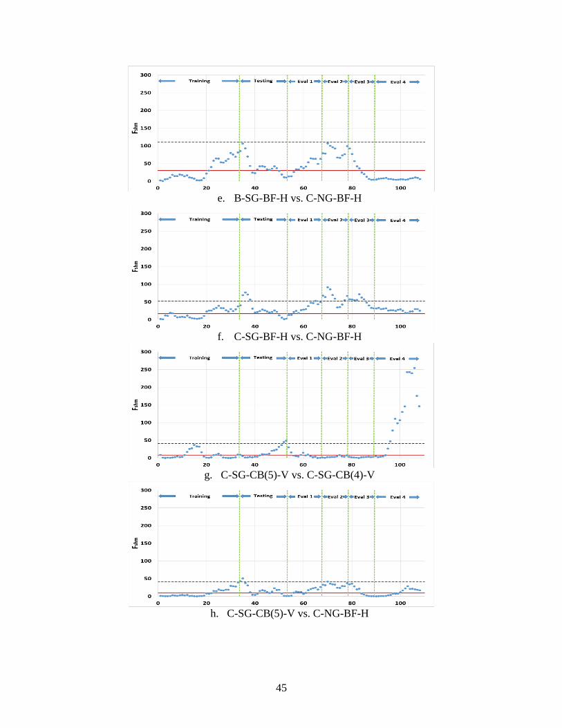
In Figure 4.8, Fshm values for global response sensors on the bridge (non-damaged) follow Rule 1

well, as data points are generally within the plus/minus three standard deviation limits. However,

as with the cross prediction method, there are a large number of false indications (Rule 1) for

sensors placed in the web cut-back region of the bridge (Sensors C-SG-CB(5)-V and

C-SG-CB(4)-V).

The number of rule violations and rates with respect to all rules were determined and are shown

in Table 4.16. A large number of rule violations are found for Rule 3 or Rule 4, as was the case

with the strain range methods and the cross prediction method.

44

a. B-NG-BF-H vs. B-SG-BF-H

b. B-NG-BF-H vs. C-SG-BF-H

c. B-NG-BF-H vs. C-SG-SB(5)-H

d. B-NG-BF-H vs. C-SG-CB(4)-V

45

e. B-SG-BF-H vs. C-NG-BF-H

f. C-SG-BF-H vs. C-NG-BF-H

g. C-SG-CB(5)-V vs. C-SG-CB(4)-V

h. C-SG-CB(5)-V vs. C-NG-BF-H

46

i. C-SG-CB(4)-V vs. C-NG-BF-H

j. B-NG-BF-H vs. Sensor 4 on sacrificial specimen

k. B-SG-BF-H vs. Sensor 1 on sacrificial specimen

l. B-SG-BF-H vs. Sensor 4 on sacrificial specimen

Figure 4.8. Fshm control chart for sacrificial Specimen 2

47

Tables 4.17 and 4.18 show the number of false indications for sensors on the bridge (non-

damaged) and on the sacrificial specimen (near damage), respectively. The Fshm method had a

higher true-indication rate than the strain range methods, as did the cross prediction method.

Table 4.17. Number of false indications for sensors on bridge (non-damaged) for Fshm

control chart

Sensor pairs

False indications

(Training, Testing,

Evaluation

1, 2, 3 and 4)

False

indication

rate

(%)

B-NG-BF-H vs. B-SG-BF-H 113 18.5

B-NG-BF-H vs. C-SG-BF-H 113 18.5

B-NG-BF-H vs. C-SG-CB(5)-V 84 13.7

B-NG-BF-H vs. C-SG-CB(4)-V 76 12.4

B-SG-BF-H vs. C-NG-BF-H 95 15.5

C-SG-BF-H vs. C-NG-BF-H 183 29.9

C-SG-CB(5)-V vs. C-SG-CB(4)-V 109 17.8

C-SG-CB(5)-V vs. C-NG-BF-H 110 18.0

C-SG-CB(4)-V vs. C-NG-BF-H 68 11.1

Table 4.18. Number of false indications for sensors on sacrificial specimen (near damage)

for Fshm control chart

Sensor pairs

near damage

False indications

(Training,

Testing,

Evaluation 1)

False

indication

rate

(%)

True

indications

(Evaluation

2, 3, and 4)

True

indication

rate

(%)

B-NG-BF-H

vs. Sensor 4 33 9.0 155 73.8

B-SG-BF-H

vs. Sensor 1 44 12.0 59 28.1

B-SG-BF-H

vs. Sensor 4 48 13.1 154 73.3

4.5 Discussion

An objective of the current study was to develop a damage-detection methodology that

minimizes the false-detection rate and maximizes the true damage-detection rate. Control chart

Rule 1 seems to best characterize the damage-detection ability for all four methodologies. The

other rules have excessively high false-indication rates and add little to the true-detection rate.

By and large, the proposed and developed four methodologies detect damage quite well. Figure

4.9 presents a comparison of the false- and true-detection rates. The false-indication rates are

48

calculated for sensors placed on the bridge where no damage was presumed to have occurred and

the true-detection rates are calculated from Sensor 4 near the crack in the sacrificial specimen.

Figure 4.9. False- and true-detection rates with Rule 1

The one-truck methodology, which is the simplest to apply and possibly the most intuitive, has

the lowest false-indication rate but also the lowest true-detection rate. The truck events grouped

by ten is similar. The two methods (cross prediction and Fshm) that pair sensors together with

orthogonal regression straight-line fits yield significant improvements in the true-detection rate

with, unfortunately, an increase in the false-indication rate.

For all methods, high false-indication rates were found from sensors (C-SG-BF(5)-V and

C-SG-BF(4)-V) placed in the cut-back web-gap region of the south girder near the west-most

pier. To help the research team understand the cause of the false-detections, the web-gap region

was inspected using visual and magnetic particle techniques.

A fatigue crack-like indication was observed as shown in Figure 4.10. As indicated in the

photograph, a small crack may be present near the sensor. The depth of the crack is not known.

Given there might be damage near the cut-back web-gap region, further investigation into the

false-indication rate was completed by omitting data from the cut-back region. The results are

illustrated in Figure 4.11.

49

Figure 4.10. Photograph of a potential fatigue crack in web cut-back region

Figure 4.11. False-indication rate without cut-back web-gap region

False-indication rates decreased for the one-truck, truck events grouped by ten, and cross

prediction methods. However, the false-detection rate for the Fshm method did not decrease

because rule violations remained in other non-damaged sensor pairs. Therefore, a challenge in

future research would be to achieve the target false-indication rate of 0.3% while maintaining a

high true-detection rate.

50

5. SUMMARY, CONCLUSIONS, AND RECOMMENDATIONS

5.1 Summary

For this project, finalization of hardware and software components for a bridge SHM system

were investigated and completed—including a demonstration installation. The goal with this

work was to ready a system for widespread implementation.

An SHM monitoring system from previous work on the US 30 Bridge used fiber-optic sensors.

In previous work, fiber-optic sensors were also placed on sacrificial specimens connected to the

bridge that simulated the structural behavior of the bridge in the cut-back gap area. Varying

degrees on damage were introduced into the sacrificial specimen. The data from the fiber-optic

system were used in this work to study the performance of four automated damage-detection

methodologies.

Although there were many advantages of the fiber-optic sensor system, the hardware system was

reconfigured with a traditional sensor system because it was found that a traditional sensor

system was more cost-effective and robust. As hoped, the traditional sensor system, installed as a

demonstration, operated without failure during the project.

An upgraded external communication system using automated FTP with 4G cellular technology

was integrated to transmit the collected data in real-time. BECAS, which is an automated

damage-detection process that incorporates sensor data acquisition, strain range data reduction

(zeroed and filtered with truck parameter identification), and statistical control charts for four

damage-detection methodologies, was developed and implemented.

The four control-chart-based methodologies developed and evaluated in this work are as follows:

1) one-truck event, 2) truck events grouped by ten, 3) cross prediction, and 4) Fshm. Control

charts utilized by the system developed are divided conceptually into three regions—training,

testing, and evaluation—to conveniently allow for study of system operability.

During the training period, strain range data from the undamaged structure were used to establish

the required control chart parameters. The testing period followed and was used to check the

efficacy of the training period. To monitor the bridge for changes in structural performance, the

evaluation period followed immediately after training and testing and was subdivided into

regions in this work corresponding to the varying damage levels in the sacrificial specimen.

Six control chart rules were applied to identify changes in structural performance with time. Rule

violations, false indications of damage in the undamaged normal structural condition, and true

indications of damage in the sacrificial specimen, with respect to each rule, were automatically

calculated and then tabulated. In all methodologies, a large number of rule violations were found

for Rule 3 and Rule 4. Rules 2, 5, and 6 had fewer false indications but also very few true

indications.

51

The one-truck event method is the most basic form of a control chart reliant upon strain range

data without further manipulation and is created using the strain range data for each truck event

without further processing. Similar to the one-truck event method, the truck events were grouped

with a group size of 10. Both the one-truck event method and the truck grouped by ten method

had relatively few false indications. Once damage was introduced into the sacrificial specimen

during the evaluation period, both were able to detect damage but with a true-indication rate less

than the other methods.

In the cross prediction method, the major enhancement over a previous generation of the

approach was in the use of orthogonal regression instead of traditional linear regression. One

attractive attribute of the cross prediction method is that it considers each sensor’s relationship

with other sensors. The cross prediction method had a higher number of false indications than the

previous two methods but a significant increase in the number of true indications.

The Fshm method is an outgrowth of a method suggested in previous work. As with the cross

prediction method, the Fshm method uses orthogonal linear regression for paired strain range data.

Unlike the first three methods, one Fshm control chart represents each pair. This results in a very

large number of control charts. The false-indication rate and true-indication rate are similar to the

cross prediction method.

5.2 Conclusions

Based on the completed work for this project, the following conclusions are made:

BECAS automates all of the components of a full SHM system successfully

As with all SHM methods, separating true structural performance data from monitoring

system noise is a major challenge and, with this work, progress has been made in this

direction by:

o Implementation of orthogonal linear regression

o Evolution of the Fshm method to improve true positive damage indications

The target false-alarm rate of 0.3% was achieved with the one-truck event method; however,

the highest true-indication rate was achieved with the Fshm method

Possible damage in the cut-back region of one girder was detected by multiple damage-

detection methods

5.3 Recommendations for Future Work

For future work, additional work is required to obtain a damage-detection methodology that

achieves the target false-indication rate (i.e., 0.3%) while at the same time ensuring a high true-

indication rate.

52

Preliminary work related to this improvement leads the research team to believe that this work

should focus on reducing the effect of strain gauge reading uncertainty. This reduction in strain

gauge uncertainty fits well in the previously-completed work aimed at decreasing uncertainty

associated with selecting live load events meeting specific criteria.

53

REFERENCES

Caragea, Petruta C. The F-Test as a Comparison of Full and Reduced Models. Iowa State

University. Ames, Iowa. Fall 2007.

Carroll, R. J., and D., Ruppert. “The Use and Misuse of Orthogonal Regression Estimation in

Linear Errors-in-Variables Models.” The American Statistician, 1996.

Doornink, J. D. Monitoring the Structural Condition of Fracture‐Critical Bridges Using Fiber

Optic Technology. PhD dissertation. Iowa State University, Ames, Iowa. 2006.

Fuller, W. A. Measurement Error Models. New York: John Wiley & Sons, Inc., 1987.

Lu, P., Phares, B. M, Greimann L., Wipf, T. J. “Bridge structural health-monitoring system using

statistical control chart analysis,” Journal of the Transportation Research Board. No.

2172, pp. 123-131, 2010.

Lu, P., A statistical based damage detection approach for highway bridge structural health

monitoring. PhD dissertation. Iowa State University. Ames, Iowa. 2008.

Mendenhall, William, and Terry Sincich. A Second Course in Statistics: Regression Analysis.

Seventh Edition. Boston, Massachusetts: Prentice Hall/Pearson Education, Inc. 2012.

Miller, I., and J. E. Freund. Probability and Statistics for Engineers. Second Edition. Englewood

Cliffs, New Jersey: Prentice-Hall, Inc.1977.

Montogomery, D. C. Introduction to Statistical Quality Control. Third Edition. New York: John

Wiley & Sons, Inc. 1996.

Phares, B., Wipf, T., Lu, P., Greimann, L., and Pohlkamp, M. An Experimental Validation of a

Statistical-Based Damage Detection Approach. Bridge Engineering Center, Iowa State

University, Ames, Iowa. 2011.

Vis, James M. Evaluation of a Structural Health Monitoring System for Steel Girder Bridges.

MS Creative Component Report. Iowa State University, Ames, Iowa. 2007.

Wipf, T. J., Phares, B. M., and Doornink, J. D. Monitoring the Structural Condition of Fracture-

Critical Bridges Using Fiber Optic Technology. Bridge Engineering Center, Iowa State

University, Ames, Iowa. 2007.

55

APPENDIX A. SPECIFICATIONS FOR THE FIBER-OPTIC SENSORS IN THE US 30

SHM SYSTEM

Channel FOS Name

Grating

length

(mm)

Central

Wavelength

(nm)

Sensor

ID

Channel 1 B-NG-BF-H 10 1517.5 1

B-NS-BF-H 10 1522.5 2

B-SS-BF-H 10 1527.5 3

B-SG-BF-H 10 1532.5 4

C-SG-BF-H 10 1537.5 5

C-FB(SS)-BF-H 10 1542.5 6

C-SS-WB-V 10 1547.5 7

C-SG-CB(5)-V 5 1552.5 8

C-SG-CB(4)-V 5 1557.5 9

C-SG-CB(3)-V 5 1562.5 10

C-SG-CB(2)-V 5 1562.5 11

C-SG-CB(1)-V 5 1567.5 12

A-NS-WB-V 10 1577.5 13

A-SS-WB-V 10 1582.5 14

Channel 2 D-SG-BF-H 10 1517.5 15

D-SS-BF-H 10 1522.5 16

D-NS-BF-H 10 1527.5 17

D-NG-BF-H 10 1532.5 18

C-NG-BF-H 10 1537.5 19

C-FB(NS)-BF-H 10 1542.5 20

C-NS-WB-V 10 1547.5 21

C-NG-CB(5)-V 5 1552.5 22

C-NG-CB(4)-V 5 1557.5 23

C-NG-CB(3)-V 5 1562.5 24

C-NG-CB(2)-V 5 1567.5 25

C-NG-CB(1)-V 5 1572.5 26

Channel 3 E-NG-BF-H 10 1517.5 27

E-NG-CB(5)-V 5 1522.5 28

E-NG-CB(1)-V 5 1527.5 29

E-NS-WB-V 10 1532.5 30

E-FB(NS)-BF-H 10 1537.5 31

E-FB(SS)-BF-H 10 1542.5 32

E-SS-WB-V 10 1547.5 33

E-SG-CB(5) 5 1552.5 34

E-SG-CB(1)-V 5 1557.5 35

E-SG-BF-H 10 1562.5 36

F-SG-BF-H 10 1567.5 37

F-SS-BF-H 10 1572.5 38

F-NS-BF-H 10 1577.5 39

F-NG-BF-H 10 1582.5 40

Channel 4 Sensor 1 5 1562 41

Sensor 2 5 1567 42

Sensor 3 5 1572 43

Sensor 4 5 1577 44

57

APPENDIX B. SETTING UP FTP DATA SYNCHRONIZATION PROCESS USING

BESTSYNC 2013

The File Transfer Protocol (FTP) data synchronization process utilized the software BestSync

2013 and the set up is described in this appendix. The first step is to set up an office FTP server

with login account information including username, password, and IP address. Next, start

BestSync and select Edit then Add Task as shown in Figure B.1.

Figure B.1. BestSync startup

Start by selecting the Folder1 magnifying glass and then select the proper Synchroniation

Direction. In most cases, select the Folder1 to Folder2 only as shown. This transfers files from

the remote desktop PC to the Office FTP Server only as shown in Figure B.2.

58

Figure B.2. File transfer

Next, select the File Folder option and choose the location where the sensor data are being stored

on the desktop computer at the remote site and finish by clicking OK as shown in Figure B.3.

Figure B.3. Data storage location

59

Subsequently, select the Folder2 magnifying glass as shown in Figure B.4.

Figure B.4. Folder destinations

Choose the FTP – File Transfer Protocol option and enter the FTP Server information as shown

in Figure B.5 and click OK.

60

Figure B.5. FTP server info

Afterward, give the task a name and click Next as shown in Figure B.6.

Figure B.6. Task name

A backup option may be specified. However, in most cases this option will not be used so

uncheck the Enable box as shown in Figure B.7.

61

Figure B.7. Backup option

Next, add any specific excludes or includes. Note that this part is typically left blank. as shown in

Figure B.8, and proceed by clicking Next.

Figure B.8. Exclude or include

62

This next process involves entering a file filter if different sets of logger files are located in the

data folder. First, uncheck the Include subfolders checkbox and check the Ignore the file if it is

changed and less than this…. Then, enter a number of seconds to keep the sync process from

trying to transfer files before they have been written completely from the logger. Note that this

may take some adjustment to get the proper time limits given that it depends on how fast the

logger is able to write files to the remote PC hard drive. Finally, check the Only scan the source

folder to detect if files are changed… checkbox and then click Next. As shown in Figure B.9,

this filter will only get .dat files that begin with CR9000X and the * is a wildcard option.

Figure B.9. Filter files

In the subsequent process, duplicate the checkbox settings shown in Figure B.10. The maximum

thread number can and should be adjusted to accommodate transfer rates of the internet service

being used. It is recommended to use 1 to 3 files maximum on 3G service and 1 to 8 files

maximum for broadband or 4G service. Finish by clicking Next and click next for the subsequent

window shown in Figure B.11.

63

Figure B.10. Copy options

Figure B.11. Volume shadow copy

The subsequent windows should be as shown in Figure B.12, B.13, and B.14.

64

Figure B.12. Encryption

Figure B.13. Naming

65

Figure B.14. Speed control

Depending on the data being retrieved, there are a couple of options for the timing after checking

Service Sync... The first option is to run Real-Time Sync by checking the appropriate box as

shown in Figure B.15. The second option is to select a rate that is appropriate to the logger data

collection rate, such as every minute as shown in Figure B.16.

Figure B.15. Schedule real-time sync option

66

Figure B.16. Schedule time option

Next, uncheck Record the log data for the log view window as shown in Figure B.17 and click

Next.

Figure B.17. Log

Click Finish as shown in Figure B.18.

67

Figure B.18. Application

Save the process by clicking File, Save As as shown in Figure B.19 and Save a copy of the

backup process in case it needs to be reloaded; otherwise, the process will need to be recreated

from scratch.

Figure B.19. Save