Integration of CasADi and JModelica.org

Joel Anderssonc Johan Åkessona,b Francesco Casellad Moritz DiehlcaDepartment of Automatic Control, Lund University, Sweden

bModelon AB, SwedencDepartment of Electrical Engineering and Optimization in Engineering Center (OPTEC),

K.U. Leuven, BelgiumdDipartimento di Elettronica e Informazione, Politecnico di Milano, Italy

Abstract

This paper presents the integration of two open sourcesoftwares: CasADi, which is a framework for efficientevaluation of expressions and their derivatives, and theModelica-based platform JModelica.org. The integra-tion of the tools is based on an XML format for ex-change of DAE models. The JModelica.org platformsupports export of models in this XML format, wherasCasADi supports import of models expressed in thisformat. Furthermore, we have carried out comparisonswith ACADO, which is a multiple shooting packagefor solving optimal control problems.

CasADi, in turn, has been interfaced with ACADOToolkit, enabling users to define optimal control prob-lems using Modelica and Optimica specifications, anduse solve using direct multiple shooting. In addi-tion, a collocation algorithm targeted at solving large-scale DAE constrained dynamic optimization prob-lems has been implemented. This implementation ex-plores CasADi’s Python and IPOPT interfaces, whichoffer a convenient, yet highly efficient environment fordevelopment of optimization algorithms. The algo-rithms are evaluated using industrially relevant bench-mark problems.

Keywords: Dynamic optimization, Symbolic ma-nipulation, Modelica, JModelica.org, ACADO Toolkit,CasADi

1 Introduction

High-level modeling frameworks such as Modelica arebecoming increasingly used in industrial applications.Existing modeling languages enable users to rapidlydevelop complex large-scale models. Traditionally,the main target for such models has been simulation,i.e., to define virtual experiments where a simulationsoftware computes the model response.

During the last two decades, methods for large scaledynamic optimization problems have been developed.Notably, linear and non-linear model predictive con-trol (MPC) have had a significant impact in the indus-trial community, in particular in the area of processcontrol. In MPC, an optimal control problem is solvedfor a finite horizon, and the first optimal control in-terval is applied to the plant. At the next sample, theprocedure is repeated, and the optimal control problemis solved again, based on updated state estimates. Theadvantages of MPC as compared to traditional controlstrategies are that it takes into account state and in-put constraints and that it handles systems with mul-tiple inputs and multiple outputs. Also, MPC offersmeans to trade performance and robustness by tuningof a cost function, where the importance of different,often contradictory, control objectives are encoded. Abottleneck when applying MPC strategies, in particu-lar in the case of non-linear systems, is that the com-putational effort needed to solve the optimal controlproblem in each sample is significant. Developmentof algorithms compatible with the real-time require-ments of MPC has therefore been a strong theme inthe research community, see e.g., [15, 40].

Driven by the impact of high-level modeling lan-guages in the industrial community, there have beenseveral efforts to integrate frameworks for such lan-guages with algorithms for dynamic optimization. Ex-amples include gPROMS [34], which supports dy-namic optimization of process systems models andDymola [13], which supports parameter and designoptimization of Modelica models. Several other appli-cations of dynamic optimization of Modelica modelshave been reported, e.g., [20, 35, 3, 33, 28].

This paper reports results of an effort wherethree different open source packages have been in-tegrated: JModelica.org, [2], ACADO Toolkit, [26],and CasADi, [4]. The integration relies on the XML

model exchange format previously reported in [32].Two main results are presented in the paper. Firstly,it is shown how CasADi, supporting import of thementioned XML model format, has been used to inte-grate JModelica.org with ACADO Toolkit. Secondly,a novel direct collocation method has been developedbased on the innovative symbolic manipulation fea-tures of CasADi. From a user’s perspective, bothCasADi and JModelica.org come with Python inter-faces, which makes scripting, plotting and analysis ofresults straightforward.

The benefit of integrating additional algorithms forsolution of dynamic optimization problems in theJModelica.org platform is that users may experimentwith different algorithms and choose the one that ismost suited for their particular problem. To some ex-tent, the situation is similar to that of choosing an in-tegrator for a simulation experiment, where it is wellknown that stiff systems require more sophisticatedsolvers than non-stiff systems.

The paper is organized as follows: in Section 2,background on dynamic optimization, Modelica andOptimica, ACADO and JModelica.org is given. Sec-tion 3 describes CasADi and recent extensions thereof.Section 4 reports a novel Python-based collocation im-plementation and in Section 5, benchmark results arepresented. The paper ends with a summary and con-clusions in Section 6.

2 Background

2.1 Dynamic optimization

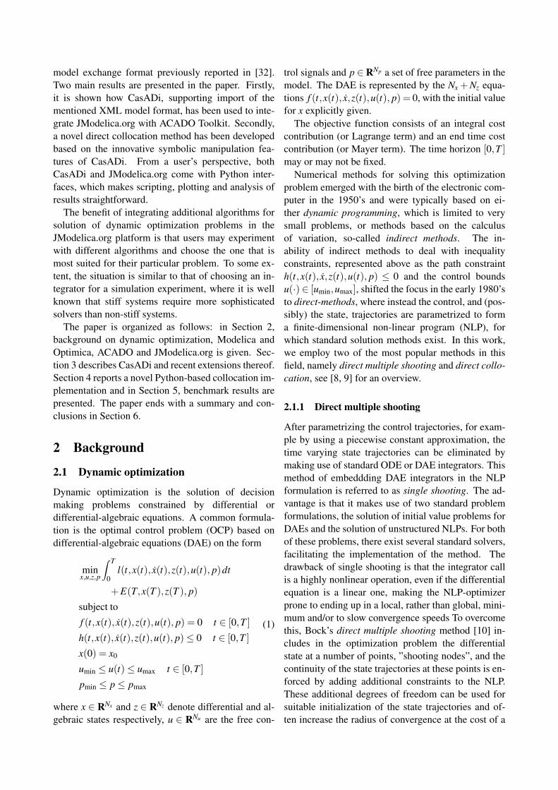
Dynamic optimization is the solution of decisionmaking problems constrained by differential ordifferential-algebraic equations. A common formula-tion is the optimal control problem (OCP) based ondifferential-algebraic equations (DAE) on the form

minx,u,z,p

∫ T

0l(t,x(t), x(t),z(t),u(t), p)dt

+E(T,x(T ),z(T ), p)subject to

f (t,x(t), x(t),z(t),u(t), p) = 0 t ∈ [0,T ]h(t,x(t), x(t),z(t),u(t), p)≤ 0 t ∈ [0,T ]x(0) = x0

umin ≤ u(t)≤ umax t ∈ [0,T ]pmin ≤ p ≤ pmax

(1)

where x ∈ RNx and z ∈ RNz denote differential and al-gebraic states respectively, u ∈ RNu are the free con-

trol signals and p ∈RNp a set of free parameters in themodel. The DAE is represented by the Nx + Nz equa-tions f (t,x(t), x,z(t),u(t), p) = 0, with the initial valuefor x explicitly given.

The objective function consists of an integral costcontribution (or Lagrange term) and an end time costcontribution (or Mayer term). The time horizon [0,T ]may or may not be fixed.

Numerical methods for solving this optimizationproblem emerged with the birth of the electronic com-puter in the 1950’s and were typically based on ei-ther dynamic programming, which is limited to verysmall problems, or methods based on the calculusof variation, so-called indirect methods. The in-ability of indirect methods to deal with inequalityconstraints, represented above as the path constrainth(t,x(t), x,z(t),u(t), p) ≤ 0 and the control boundsu(·)∈ [umin,umax], shifted the focus in the early 1980’sto direct-methods, where instead the control, and (pos-sibly) the state, trajectories are parametrized to forma finite-dimensional non-linear program (NLP), forwhich standard solution methods exist. In this work,we employ two of the most popular methods in thisfield, namely direct multiple shooting and direct collo-cation, see [8, 9] for an overview.

2.1.1 Direct multiple shooting

After parametrizing the control trajectories, for exam-ple by using a piecewise constant approximation, thetime varying state trajectories can be eliminated bymaking use of standard ODE or DAE integrators. Thismethod of embeddding DAE integrators in the NLPformulation is referred to as single shooting. The ad-vantage is that it makes use of two standard problemformulations, the solution of initial value problems forDAEs and the solution of unstructured NLPs. For bothof these problems, there exist several standard solvers,facilitating the implementation of the method. Thedrawback of single shooting is that the integrator callis a highly nonlinear operation, even if the differentialequation is a linear one, making the NLP-optimizerprone to ending up in a local, rather than global, mini-mum and/or to slow convergence speeds To overcomethis, Bock’s direct multiple shooting method [10] in-cludes in the optimization problem the differentialstate at a number of points, ”shooting nodes”, and thecontinuity of the state trajectories at these points is en-forced by adding additional constraints to the NLP.These additional degrees of freedom can be used forsuitable initialization of the state trajectories and of-ten increase the radius of convergence at the cost of a

larger NLP.The main difficulty of the method, and often the

bottleneck in terms of solution times, is to efficientlyand accurately calculate first and often second or-der derivatives of the DAE integrator, needed by theNLP solver. Implementations of the method includeMUSCOD-II and the open-source ACADO Toolkit[26], used here.

2.1.2 Direct collocation

A common alternative to shooting methods is directcollocation on finite elements. Direct collocation is asimultaneous method, where both the differential andalgebraic states as well as the controls are approxi-mated by polynomials. But in contrast to multipleshooting, no integrator is used to compute the state andalgebraic profiles. Rather, the original continuous timeoptimal control problem (1) is transcribed directly intoan algebraic problem in the form of a non-linear pro-gram (NLP). This non-linear program is usually large,but is also typically very sparse. Algorithms, such asIPOPT, [39], exist that explores the sparsity structureof the resulting NLP in order to compute solutions ofthe problem in a fast and robust way.

The interpolation polynomials used to approximatethe state profiles are usually chosen to be orthogonalLagrange polynominals, and common choices for thecollocation proints include Lobatto, Radau and Gaussschemes. In this paper, Radau collocation will be used,since this scheme has the advantage of featuring a col-location point at the end of each finite element, whichmakes encoding of continuity constraint for the statesat element junction points straightforward.

The direct collocation method shares some charac-teristics with multiple shooting, since both are simulta-neous methods. For example, unstable systems can behandled, and it is easy to incorporate state and controlconstraints. There are, however, also differences be-tween multiple shooting and direct collocation. Whilea multiple shooting method typically requires compu-tation of DAE sensitivities by means of integration ofadditional differential equations, direct collocation re-lies only on evaluation of first and (if analytic Hessianis used) second order derivatives of the DAE residual.For further discussion on the pros and cons of multipleshooting and direct collocation, see [9]

2.2 Modelica and Optimica

The Modelica language targets modeling of com-plex heterogeneous physical systems, [37]. Model-

ica permits specification of models in a wide rangeof physical domains, including mechanics, thermody-namics, electronics, chemistry and thermal systems.Also, recent versions of the language support mod-eling of embedded control systems and mapping ofcontroller code to real-time control hardware. Mod-elica is object-oriented and equation-based, where theformer property provides a means to construct mod-ular and reusable models and the latter enables theuser to state declarative equations. It is worth notic-ing that both differential and algebraic equations aresupported and that there is no need, for the user, tosolve the model equations for the derivatives, which iscommon in block-based modeling frameworks. In ad-dition, Modelica supports acausal modeling, enablingexplicit modeling of physical interfaces. This featureis the foundation of the component model in Model-ica, where components can be connected to each otherin connection diagrams.

Whereas Modelica offers state-of-the-art modelingof complex physical systems, it lacks constructs forexpressing optimization problems. For simulation ap-plications, this is not a problem, but when integratingModelica models with optimization frameworks, it isinconvenient. In order to improve the support for for-mulation of optimization problems, the Optimica ex-tension [1] has been proposed. Optimica adds to Mod-elica a small number of constructs for expressing costfunctions, constraints, and what parameters and con-trols to optimize.

2.3 JModelica.org

JModelica.org is a Modelica-based open source plat-form targeting optimization simulation and analysis ofcomplex systems, [2]. The platform offers compil-ers for Modelica and Optimica, a simulation packagecalled Assimulo and a direct collocation algorithm forsolving large-scale DAE-based dynamic optimizationproblems. The user interface in JModelica.org is basedon Python, which provides means to conveniently de-velop complex scripts and applications. In particular,the packages Numpy [30], Scipy [16] and Matplotlib[27] enable the user to perform numerical computa-tions interactively.

Recent developments of the JModelica.org plat-form includes import and export of Functional Mock-up Units (FMUs) and the integration with ACADOToolkit and CasADi reported in this paper. The JMod-elica.org platform has been used in several industrialapplications, including [28, 5, 35, 31, 23, 11]

The JModelica.org compilers generate C-code in-

tended for compilation and linking with numericalsolvers. While this is a well established procedurefor compiling Modelica models, it suffers from somedrawbacks. Compiled code indeed offers very efficientevaluation of the model equations, but it also requiresthe user to regard the model as a black box. In con-trast, there are many algorithms that can make efficientuse of models expressed in symbolic form. Exam-ples include tools for control design, optimization al-gorithms, and code generation, see [12] for a detailedtreatment of this topic. In order to offer an alterna-tive format for model export, JModelica.org supportsthe XML format described in [32]. This format is anextension of the XML scheme specified by the Func-tional Mock-up Interface (FMI) specification [29] andcontains, apart from model meta data also the modelequations. The equations are given in a format that isclosely related to the expression trees that are commonin compilers. The XML export functionality is ex-plored in this paper to integrate the packages ACADOToolkit and CasADi with the JModelica.org platform.

2.4 ACADO Toolkit

ACADO Toolkit [26] is an open-source tool for au-tomatic control and dynamic optimization developedat the Center of Excellence on Optimization in En-gineering (OPTEC) at the K.U. Leuven, Belgium. Itimplements among other things Bock’s direct multipleshooting method [10], and is in particular designed tobe used efficiently in a closed loop setting for nonlin-ear model predictive control (NMPC). For this aim, ituses the real-time iteration scheme, [14], and solvesthe NLP by a structure exploiting sequential quadraticprogramming method using the active-set quadraticprogramming (QP) solver qpOASES, [18].

Compared to other tools for dynamic optimization,the focus of ACADO Toolkit has been to develop acomplete toolchain, from the DAE integration to thesolution of optimal control problems in realtime. Thisvertical integration, together with its implementationin self-contained C++ code, allows for the tool to beefficiently deployed on embedded systems for solvingoptimization-based control and estimation problems.

3 CasADi

CasADi is a minimalistic computer algebra system im-plementing automatic differentiation, AD (see [22]) inforward and adjoint modes by means of a hybrid sym-bolic/numeric approach, [4]. It is designed to be a low-

level tool for quick, yet highly efficient implementa-tion of algorithms for numerical optimization, as il-lustrated in this paper, see Section 4. Of particularinterest is dynamic optimization, using either a col-location approach, or a shooting-based approach us-ing embedded ODE/DAE-integrators. In either case,CasADi relieves the user from the work of efficientlycalculating the relevant derivative or ODE/DAE sen-sitivity information to an arbitrary degree, as neededby the NLP solver. This together with an interfaceto Python, see Section 3.1, drastically reduces the ef-fort of implementing the methods compared to a pureC/C++/Fortran approach.

Whereas conventional AD tools are designed to beapplied black-box to C or Fortran code, CasADi al-lows the user to build up symbolic representations offunctions in the form of computational graphs, andthen apply the automatic differentiation code to thegraph directly. These graphs are allowed to be moregeneral than those normally used in AD tools, includ-ing (sparse) matrix-valued operations, switches andintegrator calls. To prevent that this added general-ity comes to the cost of lower numerical efficiency,CasADi also includes a second, more restricted graphformulation with only scalar, built-in unary and binaryoperations and no branches, similar to the ones foundin conventional AD tools.

CasADi is an open source tool, written as a self-contained C++ code, relying only on the standard tem-plate library.

3.1 Python interface to CasADi

Whereas the C++ language is highly efficent for highperformance calculations, and well suited for integra-tion with numerical packages written in C or Fortran,it lacks the interactivity needed for rapid prototypingof new mathematical algorithms, or applications of anexisting algorithm to a particular model. For this pur-pose, a scripting language such as Python, [36], or anumerical computing environment such as Matlab, ismore suitable. We choose here to work with Pythonrather than Matlab due to its open source availabiliyand ease of interfacing with other programming lan-guages.

Interfacing C++ with Python can be done in sev-eral ways. One way is to wrap the C++ classes inC functions and blend them into a Python-to-C com-piler such as Cython. While this approach is simpleenough for small C++ classes, it becomes prohibitivelycumbersome for more complex classes. Fortunately,there exist excellent tools that are able to automate

this process, such as the Simplified Wrapper and Inter-face Generator (SWIG) [17, 6] and the Boost-Pythonpackage. We have chosen to work with SWIG due toSWIG’s support for a large subset of C++ constructs, alarge and active development community and the pos-sibility to interface the code to a variety of languagesin addition to Python, in particular JAVA and Octave.

The latest version of SWIG at the time of writ-ing, version 2.0, maps C++ language constructs ontoequivalent Python constructs. Examples of featuresthat are supported in SWIG are polymorphism, excep-tions handling, templates and function overloading.

By carefully designing the CasADi C++ sourcecode, it was possible to automatically generate inter-face code for all the public classes of CasADi. Sincethe interface code is automatically generated, it iseasy to maintain as the work on CasADi progresseswith new features being added. Using CasADi fromPython renders little or no speed penalty, since virtu-ally all work-intensive calculations (numerical calcu-lation, operations on the computational graphs etc.),take place in the built-in virtual machine. Functionsformulated in Python are typically called only once,to build up the graph of the functions, thereafter thespeed penalty is neglible.

3.2 The CasADi interfaces to numerical soft-ware

In addition to being a modeling environment and anefficient AD environment, CasADi offers interfaces toa set of numeric software packages, in particular:

• The sensitivity capable ODE and DAE integratorsCVODES and IDAS from the Sundials suite [25]

• The large-scale, primal-dual interior point NLPsolver IPOPT [39]

• The ACADO toolkit

In the Sundials case, CasADi automatically formu-lates the forward or adjoint sensitivity equations andprovides Jacobian information with the appropriatesparsity needed by the linear solvers, normally an in-volved and error prone process. For IPOPT, the gra-dient of the objective function is generated via adjointAD. Also, a sparse Jacobian of the NLP constraintsas well as an exact sparse Hessian of the Lagrangiancan be generated using AD by source code transfor-mation. The ACADO Toolkit interface makes it pos-sible to use the tool from Python and attach an arbi-trary ODE/DAE integrator (currently CVODES, IDAS

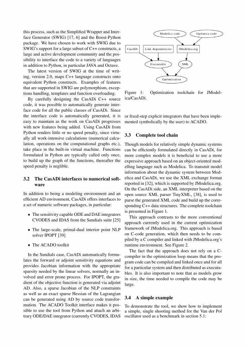
Figure 1: Optimization toolchain for JModel-ica/CasADi.

or fixed-step explicit integrators that have been imple-mented symbolically by the user) to ACADO.

3.3 Complete tool chain

Though models for relatively simple dynamic systemscan be efficiently formulated directly in CasADi, formore complex models it is beneficial to use a moreexpressive approach based on an object-oriented mod-elling language such as Modelica. To transmit modelinformation about the dynamic system between Mod-elica and CasADi, we use the XML exchange formatreported in [32], which is supported by JModelica.org.On the CasADi side, an XML interpreter based on theopen source XML parser TinyXML, [38], is used toparse the generated XML code and build up the corre-sponding C++ data structures. The complete toolchainis presented in Figure 1.

This approach contrasts to the more conventionalapproach currently used in the current optimizationframework of JModelica.org. This approach is basedon C-code generation, which then needs to be com-piled by a C compiler and linked with JModelica.org’sruntime environment. See Figure 2.

The fact that the approach does not rely on a C-compiler in the optimization loop means that the pro-gram code can be compiled and linked once and for allfor a particular system and then distributed as executa-bles. It is also important to note that as models growin size, the time needed to compile the code may belarge.

3.4 A simple example

To demonstrate the tool, we show how to implementa simple, single shooting method for the Van der Poloscillator used as a benchmark in section 5.1:

Figure 2: Optimization toolchain for JModelica.

from casadi import *

# Declare variables (use simple, efficient DAG)

t = SX("t") # time

x=SX("x"); y=SX("y"); u=SX("u"); L=SX("cost")

# ODE right hand side function

f = [(1 - y*y)*x - y + u, x, x*x + y*y + u*u]

rhs = SXFunction([[t],[x,y,L],[u]],[f])

# Create an integrator (CVODES)

I = CVodesIntegrator(rhs)

I.setOption("ad_order",1) # enable AD

I.setOption("abstol",1e-10) # abs. tolerance

I.setOption("reltol",1e-10) # rel. tolerance

I.setOption("steps_per_checkpoint",1000)

I.init()

# Number of control intervals

NU = 20

# All controls (use complex, general DAG)

U = MX("U",NU) # NU-by-1 matrix variable

# The initial state (x=0, y=1, L=0)

X = MX([0,1,0])

# Time horizon

T0 = MX(0); TF = MX(20.0/NU)

# State derivative and algebraic state

XP = MX(); Z = MX() # Not used

# Build up a graph of integrator calls

for k in range(NU):

[X,XP,Z] = I.call([T0,TF,X,U[k],XP,Z])

# Objective function: L(T)

F = MXFunction([U],[X[2]])

# Terminal constraints: 0<=[x(T);y(T)]<=0

G = MXFunction([U],[X[0:2]])

solver = IpoptSolver(F,G)

solver.setOption("tol",1e-5)

solver.setOption("hessian_approximation", \

"limited-memory")

solver.setOption("max_iter",1000)

solver.init()

# Set bounds and initial guess

solver.setInput(NU*[-0.75], NLP_LBX)

solver.setInput(NU*[1.0],NLP_UBX)

solver.setInput(NU*[0.0],NLP_X_INIT)

solver.setInput([0,0],NLP_LBG)

solver.setInput([0,0],NLP_UBG)

# Solve the problem

solver.solve()

In CasADi, symbolic variables are instances of ei-ther the scalar expression class SX, or the more generalmatrix expression class MX.

x=SX("x"); y=SX("y"); u=SX("u"); L=SX("cost")

...

U = MX("U",NU) # NU-by-1 matrix variable

In the example above, we declare variables and for-mulate the right-hand-side of the integrator symboli-cally:

f = [(1 - y*y)*x - y + u, x, x*x + y*y + u*u]

Note that at the place where this is encountered inthe script, neither x, y or u have taken a particularvalue. This representation of the ordinary differen-tial equation is passed to the ODE integrator CVODESfrom the Sundials suite [25]. Since the ODE is in sym-bolic form, the integrator interface is able to derive anyinformation it might need to be able to solve the initialvalue problem efficiently, relieving the user of a te-dious and often error prone process. The informationthat can be automatically generated includes derivativeinformation for sparse, dense or banded methods, aswell as the formulation of the forward and adjoint sen-sitivity equations (required here since the integrator isbeing used in an optimal control setting).

The next interesting line is:

for k in range(NU):

[X,XP,Z] = I.call([T0,TF,X,U[k],XP,Z])

Here, the call member function of theCVodesIntegrator instance is used to constructa graph with function calls to the integrator. Since the

matrix variable U is not known at this point, actuallysolving the IVP is not possible. This allows us to geta completely symbolic representation not only of theODE, but of the nonlinear programming program.We then pass the NLP to the open source dual-primalinterior point NLP solver IPOPT. Again, since theformulation is symbolic, the IPOPT interface willgenerate all the information it needs to solve theproblem, including the gradient of the NLP objectivefunction and the Jacobian of the NLP constraintfunction, both of which can be best calculated usingautomatic differentiation in adjoint mode for thisparticular example.

Note that the example above, with comments re-moved, consists of about 30 lines of code, which isa very compact way to implement the single shoot-ing method. With only moderately more effort, othermethods from the field of optimal control can be for-mulated including multiple-shooting and direct col-location, see Section 4. When executing the scriptabove, it iterates to the the correct solution in 592 NLPiterations, which is considerably slower than the corre-sponding results for the simultaneous methods. Adapt-ing the script to implement multple-shooting ratherthan single-shooting (the code of which is available inCasADi’s example collection), decreases the numberof NLP iterations to only 17.

4 A Python-based Collocation Algo-rithm

As described in Section 2.1, one strategy for solv-ing large-scale dynamic optimization problems is di-rect collocation, where the dynamic DAE constraintis replaced by a discrete time approximation. The re-sult is an non-linear program (NLP), which can besolved with standard algorithms. A particular chal-lenge when implementing collocation algorithms isthat the algorithms typically used to solve the result-ing NLP require accurate derivative information andsparsity structures. In addition, second order deriva-tives can often improve robustness and convergence ofsuch algorithms.

One option for implementing collocation algorithmis provided by optimization tools such as AMPL [19]and GAMS [21]. These tools support formulation oflinear and non-linear programs and the user may spec-ify collocation problems by encoding the model equa-tions as well as the collocation constraints. The AMPLplatform also provides a solver API, supporting evalu-ation of the cost function and the constraints, as well

as first and second order derivatives, including sparsityinformation. A benefit for the user is that the tool in-ternally computes these quantities using an automaticdifferentiation strategy that is very efficient, which inturn enables a solver algorithm to operate fast and reli-ably. On the other hand, AMPL, and similar systems,does not offer appropriate support for physical mod-eling. The description format is inherently flat, whichmakes construction of reusable models intractable.

Physical modeling systems, on the other hand, of-fer excellent support for modeling and model reuse,but typically offer only model execution interfacesthat often do not provide all the necessary API func-tions. Typically, sparsity information and second or-der derivative information is lacking. The model exe-cution interface in JModelica.org, entitled the JMod-elica.org Model Interface (JMI) overcomes some ofthese deficiencies by providing a DAE interface sup-porting sparse Jacobians, which in turn are computedusing the CppAD package [7]. Based on JMI, a directcollocation algorithm has been implemented in C andthe resulting NLP has been interfaced with the algo-rithm IPOPT [39]. While this approach has been suc-cessfully used in a number of industrially relevant ap-plications, it also requires a significant effort in termsof implementation and maintenance. In many respects,implementation of collocation algorithms reduces tobook keeping problems where indices of states, inputsand parameters need to be tracked in the global vari-able vector. Also, the sparsity structure of the DAE Ja-cobian needs to be mapped into the composite NLP re-sulting from collocation. In this respect, the approachtaken in AMPL and GAMS has significant advantages.

In an effort to explore the strengths of the physi-cal modeling framework JModelica.org and the con-venience and efficiency in evaluation of derivatives of-fered by CasADi, a direct collocation algorithm simi-lar to the one existing in JModelica.org has been im-plemented. The implementation is done completelyin Python relying on CasADi’s model import featureand its Python interface. As compared to the approachtaken with AMPL, the user is relieved from the bur-den of implementing the collocation algorithm itself.In this respect the new implementation does not dif-fer from the current implementation in JModelica.org,but instead, the effort needed to implement the algo-rithm is significantly reduced. Also, advanced usersmay easily tailor the collocation algorithm to their spe-cific needs.

The implementation used for the benchmarks pre-sented in this paper is a third order Radau scheme,

which is also supported by the C collocation imple-mentation in JModelica.org.

5 Benchmarks

Three different optimal control benchmark problemswith different properties have been selected for com-parison of the different algorithms: the Van der Pol os-cillator, a Continuously Stirred Tank Reactor (CSTR)with an exothermic reaction, and a combined cyclepower plant. The first bencmark, the Van der Pol oscil-lator, is a system commonly studied in non-linear con-trol courses, and demonstrates the ability of all meth-ods evaluated to solve optimal control problems. TheCSTR problem features highly non-linear dynamics incombination with a state contstraint. The final bench-mark, the combined cycle power plant, is of largerscale, consisting of nine states and more than 100 al-gebraics.

Whereas the Van der Pol problem has been success-fully solved using both multiple shooting and collo-cation, a solution to the CSTR and combined cycleproblem has been obtained only using a collocationapproach.

For reference, the original collocation implementa-tion, written in C, is included in the benchmarks. Thisalgorithm is referred to as JM collocation.

All the calculations have been performed on an DellLatitude E6400 laptop with an Intel Core Duo proces-sor of 2.4 GHz, 4 GB of RAM, 3072 KB of L2 Cacheand 128 kB if L1 cache, running Linux.

In the benchmarks where IPOPT is used, the algo-rithm is compiled with the linear solver MA57 fromthe HSL suite.

5.1 Optimal control of the Van der Pol Oscil-lator

As a first example, consider the Van der Pol oscillator,described by the differential equations

x1 = x2, x1(0) = 1

x2 = (1− x21)x2− x1 x2(0) = 0.

(2)

The optimization problem is formulated as to mini-mize the following cost

minu

∫ 20

0x2

1 + x22 +u2dt (3)

subject to the constraint

u ≤ 0.75. (4)

Figure 3: Optimization results for the Van der Pol os-cillator.

First, we solve the optimal control problem using threedifferent algorithms, all based on the Modelica modeland the Optimica specification encoding the optimalcontrol problem. 20 uniformly distributed controlsegements were used in all cases. The first methodused to solve the problem is JModelica’s native, C-based implementation of direct collocation, which re-lies on code generation and the AD-tool CppAD togenerate derivatives. Secondly, the novel, CasADiand Python-based implementation of direct colloca-tion presented in Section 4 is applied. The third al-gorithm is ACADO Toolkit’s implementation of mul-tiple shooting, using CasADi’s interface to evaluatefunctions and and directional derivatives. Forwardmode AD was used to generate DAE sensitivities and aBFGS approximation of the Hessian of the Lagrangianof the NLP. The optimal solutions for the three differ-ent algorithms are shown in Figure 3.

Table 1 shows the number of NLP iterations andtotal CPU time for the optimization (in seconds) for5 different algorithmic approaches: direct colloca-tion implemented in C and in Python using CasADi,ACADO Toolkit via the CasADi interface, and imple-mentations of single and multiple shooting based onCasADi’s Python interface. The implementations ofsingle and multiple shooting are included to demon-strate usage of CasADi’s integrator and NLP solverimplementation, rather than to achive high perfor-mance. For the single shooting code, the completescript was presented in Section 3.4.

The last column of the table contains the share of the

total time spent in the NLP solver, the rest is mostlyspent in the DAE functions (DAE residual, Jacobianof the constraints, objective function etc.) which areinterfaced to the NLP solver. This information is notavailable for ACADO Toolkit.

Table 1: Execution times for the Van der Pol bench-mark.

Tool NLPitera-tions

Totaltime [s]

Timein NLPsolver[s]

JModelica.org coll. 21 0.32 0.14CasADi collocation 103 0.97 0.92ACADO via CasADi 28 3.45 n/aCasADi single shooting 616 167.7 1.22CasADi mult. shooting 16 59.1 0.20

We can see that JModelica’s current C-based imple-mentation of direct collocation and ACADO’s multi-ple shooting implementation, both of them using aninexact Hessian approximation with BFGS updating,show a similar number of NLP iterations. In terms ofspeed, the JModelica.org implementation clearly out-performs ACADO which is at least partly explainedby the fact that JModelica.org involves a code genera-tion step, significantly reducing the function overheadin the NLP solver. Also, CasADi involves a code gen-eration step, but not to C-code which is then compiled,but to a virtual machine implemented inside CasADi.Clearly, this virtual machine is able to compete withthe C implementation in terms of efficiently duringevaluation and is also fast in the translation phase, asno C-code needs to be generated and compiled. Alsonote that for this small problem size, the function over-head associated with calling the DAE right hand sideis major for all of the shooting methods. A more faircomparison here would involve the use of ACADOToolkit’s own symbolic syntax coupled with a codegeneration step in ACADO.

In this particular example, IPOPT, using CasADi togenerate the exact Hessian of the Lagrangian, requiremore NLP steps than ACADO and JModelica.org’snative implementation of collocation which are bothusing an inexact Hessian approximation. Despite thefact that the CasADi-based implementation does notrely on C code generation, and although it is calculat-ing the exact Hessian, the time it takes to evaluate thefunctions only constitute only a small fraction (around5%) of the total execution time. In contrast, in the C-based implmentation, the time spent in DAE functions,make up more than half of the total CPU time. This re-sult cleary demonstrates one of the main strengths of

CasADi, namely computational efficiency.Looking at the number of iterations required in the

single shooting algorithm, the superior convergencespeed of simultaneous methods (collocation and mul-tiple shooting) is obvious.

5.2 Optimal control of a CSTR reactor

We consider the Hicks-Ray Continuously Stirred TankReactor (CSTR) containing an exothermic reaction,[24]. The states of the system are the reactor temper-ature T and the reactant concentration c. The reactantinflow rate, F0, concentration, c0, and temperature, T0,are assumed to be constant. The input of the system isthe cooling flow temperature Tc. The dynamics of thesystem is then given by:

c(t) = F0(c0− c(t))/V − k0e−EdivR/T (t)c(t)T (t) = F0(T0−T (t))/V−

dH/(ρCp)k0e−EdivR/T (t)c(t)+2U/(rρCp)(Tc(t)−T (t))

(5)

where r, k0, EdivR, U , ρ , Cp, dH, and V are physicalparameters.

Based on the CSTR model, the following dynamicoptimization problem is formulated:

minTc(t)

∫ t f

0(cref− c(t))2 +(T ref−T (t))2+

(T refc −Tc(t))2dt

(6)

subject to the dynamics (5). The cost function corre-sponds to a load change of the system and penalizesdeviations from a desired operating point given by tar-get values cref, T ref and T ref

c for c, T and Tc respec-tively. Stationary operating conditions were computedbased on constant cooling temperatures Tc = 250 (ini-tial conditions) and Tc = 280 (reference point).

In order to avoid too high temperatures during theignition phase of the reactor, the following tempera-ture bound was enforced:

T (t)≤ 350. (7)

The optimal trajectories for the three different al-gorithms are shown in Figure 4, where we have useda control discretization of 100 elements and a 3rd or-der Radau-discretization of the state trajectories for thetwo collocation implementations.

Table 2 shows the performance of the two comparedimplementations of collocation in terms of NLP itera-tions and CPU time.

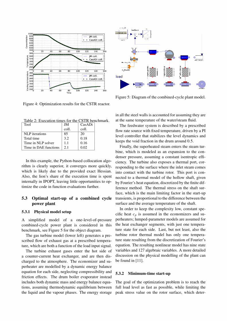
Figure 4: Optimization results for the CSTR reactor.

Table 2: Execution times for the CSTR benchmark.Tool JM

coll.CasADicoll.

NLP iterations 85 20Total time 3.2 0.18Time in NLP solver 1.1 0.16Time in DAE functions 2.1 0.02

In this example, the Python-based collocation algo-rithm is clearly superior, it converges more quickly,which is likely due to the provided exact Hessian.Also, the lion’s share of the execution time is spentinternally in IPOPT, leaving little opportunities to op-timize the code in function evaluations further.

5.3 Optimal start-up of a combined cyclepower plant

5.3.1 Physical model setup

A simplified model of a one-level-of-pressurecombined-cycle power plant is considered in thisbenchmark, see Figure 5 for the object diagram.

The gas turbine model (lower left) generates a pre-scribed flow of exhaust gas at a prescribed tempera-ture, which are both a function of the load input signal.

The turbine exhaust gases enter the hot side ofa counter-current heat exchanger, and are then dis-charged to the atmosphere. The economizer and su-perheater are modelled by a dynamic energy balanceequation for each side, neglecting compressibility andfriction effects. The drum boiler evaporator insteadincludes both dynamic mass and energy balance equa-tions, assuming thermodynamic equilibrium betweenthe liquid and the vapour phases. The energy storage

Figure 5: Diagram of the combined-cycle plant model.

in all the steel walls is accounted for assuming they areat the same temperature of the water/steam fluid.

The feedwater system is described by a prescribedflow rate source with fixed temperature, driven by a PIlevel controller that stabilizes the level dynamics andkeeps the void fraction in the drum around 0.5.

Finally, the superheated steam enters the steam tur-bine, which is modeled as an expansion to the con-denser pressure, assuming a constant isentropic effi-ciency. The turbine also exposes a thermal port, cor-responding to the surface where the inlet steam comesinto contact with the turbine rotor. This port is con-nected to a thermal model of the hollow shaft, givenby Fourier’s heat equation, discretized by the finite dif-ference method. The thermal stress on the shaft sur-face, which is the main limiting factor in the start-uptransients, is proportional to the difference between thesurface and the average temperature of the shaft.

In order to keep the complexity low, constant spe-cific heat cp is assumed in the economizers and su-perheaters; lumped-parameter models are assumed forthe heat exchanger segments, with just one tempera-ture state for each side. Last, but not least, also theturbine rotor thermal model has only one tempera-ture state resulting from the discretization of Fourier’sequation. The resulting nonlinear model has nine statevariables and 127 algebraic variables. A more detaileddiscussion on the physical modelling of the plant canbe found in [11].

5.3.2 Minimum-time start-up

The goal of the optimization problem is to reach thefull load level as fast as possible, while limiting thepeak stress value on the rotor surface, which deter-

mines the lifetime consumption of the turbine. Sincethe steam cycle is assumed to operate in a pure slid-ing pressure mode, the full load state is reached whenthe load level of the turbine, u(t) (which is the con-trol variable), has reached 100% and the normalizedvalue of the evaporator pressure, pev, has reached thetarget reference value pref

ev . A Lagrange-type cost func-tion, penalizing the sum of the squared deviations fromthe target values, drives the system towards the desiredset-point (pevap,u) = (pref

evap,1) as quickly as possible.Inequality constraints are prescribed on the maxi-

mum admissible thermal stress in the steam turbine,σ(t), as well as on the rate of change of the gas turbineload: on one hand, the load is forbidden to decrease,in order to avoid cycling of the stress level during thetransient; on the other hand, it cannot exceed the max-imum rate prescribed by the manufacturer.

The start-up optimization problem is then definedas:

minu(t)

∫ t f

t0(pevap(t)− pref

evap)2 +(u(t)−1)2 dt (8)

subject to the constraints

σ(t)≤ σmax

u(t)≤ dumin

u(t)≥ 0

(9)

and to the DAE dynamics representing the plant.The initial state for the DAE represents the state ofthe plant immediately after the steam turbine roll-outphase and the connection of the electric generator tothe grid.

The optimization result is shown in Figure 6. Dur-ing the first 200 seconds, the gas turbine load is in-creased at the maximum allowed rate and the stressbuilds up rapidly, until it reaches the target limit. Sub-sequently, the load is slowly increased, in order tomaintain the stress level approximately constant at theprescribed limit. When the 50% load level is reached,further increases of the load do not cause additionalincrease of the gas exhaust temperature, and thereforecause only small increases of the steam temperature.It is then possible to resume increasing the load at themaximum allowed rate, while the stress level starts todecrease. The full load is reached at about 1400 s. Be-tween 1000 and 1100 seconds, the load increase rateis actually zero; apparently, this small pause allows toincrease the load faster later on, leading to an overallshorter start-up time.

This problem, which is of a more realistic size hasbeen solved with the two direct collocation implemen-tations and the results are shown in Table 3.

Figure 6: Optimal startup of a combined cycle powerplant.

Table 3: Execution times for the combined cyclebenchmark.

Tool JM coll CasADicoll

NLP iterations 49 198Total time 19.9 16.3Time in NLP solver 2.4 15.3Optimal cost 6487 6175

We note that the CasADi-based collocation algo-rithm needs more iterations to reach the optimal solu-tion, but on the other hand, the optimum that it found isindeed better than the one found using BFGS. Whetherthis is due to some minor differences in the collocationalgorithms (since the models are identical), is beyondthe scope of this paper. What can be said with certaintyis that whereas most of the time spent in the DAE func-tions in the existing C-based approach, the oppositeis true for the CasADi approach. Indeed, with morethan 90% of the computational time spent internally inIPOPT, optimizing the CasADi execution time furtherwould do little to reduce the overall execution time.

6 Summary and Conclusions

In this paper, the integration of CasADi and the JMod-elica.org platform has been reported. It has beenshown how an XML-based model exchange formatsupported by JModelica.org and CasADi is used tocombine the expressive power provided by Modelicaand Optimica with state of the art optimization algo-rithms. The use of a language neutral model exchangeformat simplifies tool interoperability and allows users

to use different optimization algorithms without theneed to reencode the problem formulation. As com-pared to traditional optimization frameworks, typicallyrequiring user’s to encode the model, the cost functionand the constraints in a algorithm-specific manner, theapproach put forward in this paper increases flexibilitysignificantly.

7 Acknowledgments

This research at KU Leuven was supportedby the Research Council KUL via the Centerof Excellence on Optimization in EngineeringEF/05/006 (OPTEC, http://www.kuleuven.be/optec/),GOA AMBioRICS, IOF-SCORES4CHEM andPhD/postdoc/fellow grants, the Flemish Governmentvia FWO (PhD/postdoc grants, projects G.0452.04,G.0499.04, G.0211.05,G.0226.06, G.0321.06,G.0302.07, G.0320.08, G.0558.08, G.0557.08, re-search communities ICCoS, ANMMM, MLDM) andvia IWT (PhD Grants, McKnow-E, Eureka-Flite+),Helmholtz Gemeinschaft via vICeRP, the EU viaERNSI, Contract Research AMINAL, as well asthe Belgian Federal Science Policy Office: IUAPP6/04 (DYSCO, Dynamical systems, control andoptimization, 2007-2011).

Johan Åkesson gratefully acknowledges financialsupport from the Swedish Science Foundation throughthe grant Lund Center for Control of Complex Engi-neering Systems (LCCC).

References

[1] Johan Åkesson. Optimica—an extension of mod-elica supporting dynamic optimization. In In 6thInternational Modelica Conference 2008. Mod-elica Association, March 2008.

[2] Johan Åkesson, Karl-Erik Årzén, Mag-nus Gäfvert, Tove Bergdahl, and HubertusTummescheit. Modeling and optimization withOptimica and JModelica.org—languages andtools for solving large-scale dynamic optimiza-tion problem. Computers and Chemical Engi-neering, 34(11):1737–1749, November 2010.Doi:10.1016/j.compchemeng.2009.11.011.

[3] Johan Åkesson and Ola Slätteke. Modeling, cali-bration and control of a paper machine dryer sec-tion. In 5th International Modelica Conference2006, Vienna, Austria, September 2006. Model-ica Association.

[4] J. Andersson, B. Houska, and M. Diehl. Towardsa Computer Algebra System with Automatic Dif-ferentiation for use with Object-Oriented mod-elling languages. In 3rd International Work-shop on Equation-Based Object-Oriented Mod-eling Languages and Tools, Oslo, Norway, Octo-ber 3, 2010.

[5] Niklas Andersson, Per-Ola Larsson, JohanÅkesson, Staffan Haugwitz, and Bernt Nilsson.Calibration of a polyethylene plant for gradechange optimizations. In 21st European Sympo-sium on Computer-Aided Process Engineering,May 2011. Accepted for publication.

[6] D. M. Beazley. Automated scientific softwarescripting with SWIG. Future Gener. Comput.Syst., 19:599–609, July 2003.

[7] B. M. Bell. CppAD Home Page, 2010. http:

//www.coin-or.org/CppAD/.

[8] Lorenz T. Biegler. Nonlinear programming: con-cepts, algorithms, and applications to chemicalprocesses. SIAM, 2010.

[9] T. Binder, L. Blank, H.G. Bock, R. Bulirsch,W. Dahmen, M. Diehl, T. Kronseder, W Mar-quardt, J.P. Schlöder, and O. v. Stryk. Online Op-timization of Large Scale Systems, chapter Intro-duction to model based optimization of chemicalprocesses on moving horizons, pages 295–339.Springer-Verlag, Berlin Heidelberg, 2001.

[10] H.G. Bock and K.J. Plitt. A multiple shoot-ing algorithm for direct solution of optimal con-trol problems. In Proceedings 9th IFAC WorldCongress Budapest, pages 243–247. PergamonPress, 1984.

[11] F. Casella, F. Donida, and J. Åkesson. Object-oriented modeling and optimal control: A casestudy in power plant start-up. In Proc. 18th IFACWorld Congress, 2011. In submission.

[12] Francesco Casella, Filippo Donida, and JohanÅkesson. An XML representation of DAE sys-tems obtained from Modelica models. In Pro-ceedings of the 7th International Modelica Con-ference 2009. Modelica Association, September2009.

[13] Dassault Systemes. Dymola web page, 2010.http://www.3ds.com/products/catia/

portfolio/dymola.

[14] M. Diehl, H.G. Bock, J.P. Schlöder, R. Findeisen,Z. Nagy, and F. Allgöwer. Real-time optimiza-tion and Nonlinear Model Predictive Controlof Processes governed by differential-algebraicequations. J. Proc. Contr., 12(4):577–585, 2002.

[15] M. Diehl, H. J. Ferreau, and N. Haverbeke. Non-linear model predictive control, volume 384 ofLecture Notes in Control and Information Sci-ences, chapter Efficient Numerical Methods forNonlinear MPC and Moving Horizon Estima-tion, pages 391–417. Springer, 2009.

[16] Inc. Enthought. SciPy, 2010. http://www.

scipy.org/.

[17] Dave Beazley et al. SWIG – Simplified Wrap-per and Interface Generator, version 2.0, 2010.http://www.swig.org/.

[18] H. J. Ferreau, H. G. Bock, and M. Diehl. Anonline active set strategy to overcome the limita-tions of explicit MPC. International Journal ofRobust and Nonlinear Control, 18(8):816–830,2008.

[19] R Fourer, D. Gay, and B Kernighan. AMPL – AModeling Language for Mathematical Program-ming. Brooks/Cole — Thomson Learning, 2003.

[20] R. Franke, M. Rode, and K Krü 12 ger. On-line op-

timization of drum boiler startup. In Proceedingsof Modelica’2003 conference, 2003.

[21] Gams Development Corporation. GAMS webpage, 2010. http://www.gams.com/.

[22] A. Griewank. Evaluating Derivatives, Principlesand Techniques of Algorithmic Differentiation.Number 19 in Frontiers in Appl. Math. SIAM,Philadelphia, 2000.

[23] Staffan Haugwitz, Johan Åkesson, and Per Ha-gander. Dynamic start-up optimization of a platereactor with uncertainties. Journal of ProcessControl, 19(4):686–700, April 2009.

[24] G. A. Hicks and W. H. Ray. Approximationmethods for optimal control synthesis. Can. J.Chem. Eng., 20:522 –529, 1971.

[25] A. C. Hindmarsh, P. N. Brown, K. E. Grant, S. L.Lee, R. Serban, D. E. Shumaker, and C. S. Wood-ward. Sundials: Suite of nonlinear and differ-ential/algebraic equation solvers. ACM Trans-actions on Mathematical Software, 31:363–396,2005.

[26] B. Houska, H.J. Ferreau, and M. Diehl. ACADOToolkit – An Open Source Framework for Auto-matic Control and Dynamic Optimization. Op-timal Control Applications and Methods, 2010.DOI: 10.1002/oca.939 (in print).

[27] J. Hunter, D. Dale, and M. Droettboom. Mat-PlotLib: Python plotting, 2010. http://

matplotlib.sourceforge.net/.

[28] P-O. Larsson, J. Åkesson, Staffan Haugwitz, andNiklas Andersson. Modeling and optimization ofgrade changes for multistage polyethylene reac-tors. In Proc. 18th IFAC World Congress, 2011.In submission.

[29] Modelisar. Functional Mock-up Interfacefor Model Exchange, 2010. http://www.

functional-mockup-interface.org.

[30] T. Oliphant. Numpy Home Page, 2009. http:

//numpy.scipy.org/.

[31] B. Olofsson, H. Nilsson, A. Robertsson, andJ. Åkesson. Optimal tracking and identificationof paths for industrial robots. In Proc. 18th IFACWorld Congress, 2011. In submission.

[32] Roberto Parrotto, Johan Åkesson, and FrancescoCasella. An XML representation of DAE sys-tems obtained from continuous-time Modelicamodels. In Third International Workshop onEquation-based Object-oriented Modeling Lan-guages and Tools - EOOLT 2010, September2010.

[33] J. Poland, A. J. Isaksson, and P. Aronsson. Build-ing and solving nonlinear optimal control and es-timation problems. In 7th International ModelicaConference, 2009.

[34] Process Systems Enterprise. gPROMS HomePage, 2010. http://www.psenterprise.com/gproms/index.html.

[35] K. Prölss, H. Tummescheit, S. Velut, Y. Zhu,J. Åkesson, and C. D. Laird. Models for a post-combustion absorption unit for use in simulation,optimization and in a non-linear model predictivecontrol scheme. In 8th International ModelicaConference, 2011.

[36] Python Software Foundation. Python Program-ming Language – Official Website, January2011. http://www.python.org/.

[37] The Modelica Association. Modelica – a uni-fied object-oriented language for physical sys-tems modeling, language specification, version3.2. Technical report, Modelica Association,2010.

[38] Lee Thomason. TinyXML, January 2011. http://www.grinninglizard.com/tinyxml/.

[39] Andreas Wächter and Lorenz T. Biegler. Onthe implementation of an interior-point filterline-search algorithm for large-scale nonlinearprogramming. Mathematical Programming,106(1):25–58, 2006.

[40] V. M. Zavala and L. T. Biegler. The advancedstep NMPC controller: Optimality, stability androbustness. Automatica, 45(1):86–93, 2009.