User Documentation for CasADi...

User Documentation for CasADi v3.2.2

Joel Andersson Joris Gillis Moritz Diehl

August 2, 2017

2

Contents

1 Introduction 5

1.1 What CasADi is and what it is not . . . . . . . . . . . . . . . . . . . . . . 5

1.2 Help and support . . . . . . . . . . . . . . . . . . . . . . . . . . . . . . . . 6

1.3 Citing CasADi . . . . . . . . . . . . . . . . . . . . . . . . . . . . . . . . . . 6

1.4 Reading this document . . . . . . . . . . . . . . . . . . . . . . . . . . . . . 6

2 Obtaining and installing CasADi 9

3 Symbolic framework 11

3.1 The SX symbolics . . . . . . . . . . . . . . . . . . . . . . . . . . . . . . . . 11

3.2 DM . . . . . . . . . . . . . . . . . . . . . . . . . . . . . . . . . . . . . . . . 13

3.3 The MX symbolics . . . . . . . . . . . . . . . . . . . . . . . . . . . . . . . . 14

3.4 Mixing SX and MX . . . . . . . . . . . . . . . . . . . . . . . . . . . . . . . . 15

3.5 The Sparsity class . . . . . . . . . . . . . . . . . . . . . . . . . . . . . . . 16

3.5.1 Getting and setting elements in matrices . . . . . . . . . . . . . . . 17

3.6 Arithmetic operations . . . . . . . . . . . . . . . . . . . . . . . . . . . . . 18

3.7 Querying properties . . . . . . . . . . . . . . . . . . . . . . . . . . . . . . . 20

3.8 Linear algebra . . . . . . . . . . . . . . . . . . . . . . . . . . . . . . . . . . 21

3.9 Calculus – algorithmic differentiation . . . . . . . . . . . . . . . . . . . . . 21

4 Function objects 23

4.1 Calling function objects . . . . . . . . . . . . . . . . . . . . . . . . . . . . 24

4.2 Converting MX to SX . . . . . . . . . . . . . . . . . . . . . . . . . . . . . . . 25

4.3 Nonlinear root-finding problems . . . . . . . . . . . . . . . . . . . . . . . . 25

4.4 Initial-value problems and sensitivity analysis . . . . . . . . . . . . . . . . 26

4.4.1 Creating integrators . . . . . . . . . . . . . . . . . . . . . . . . . . 26

4.4.2 Sensitivity analysis . . . . . . . . . . . . . . . . . . . . . . . . . . . 27

4.5 Nonlinear programming . . . . . . . . . . . . . . . . . . . . . . . . . . . . 28

4.5.1 Creating NLP solvers . . . . . . . . . . . . . . . . . . . . . . . . . . 28

4.6 Quadratic programming . . . . . . . . . . . . . . . . . . . . . . . . . . . . 29

4.6.1 High-level interface . . . . . . . . . . . . . . . . . . . . . . . . . . . 29

4.6.2 Low-level interface . . . . . . . . . . . . . . . . . . . . . . . . . . . 30

3

4 CONTENTS

5 Generating C-code 335.1 Syntax for generating code . . . . . . . . . . . . . . . . . . . . . . . . . . . 335.2 Using the generated code . . . . . . . . . . . . . . . . . . . . . . . . . . . . 355.3 API of the generated code . . . . . . . . . . . . . . . . . . . . . . . . . . . 37

6 User-defined function objects 416.1 Subclassing FunctionInternal . . . . . . . . . . . . . . . . . . . . . . . . 416.2 Subclassing Callback . . . . . . . . . . . . . . . . . . . . . . . . . . . . . . 426.3 Importing a function with external . . . . . . . . . . . . . . . . . . . . . 45

7 The DaeBuilder class 477.1 Mathematical formulation . . . . . . . . . . . . . . . . . . . . . . . . . . . 477.2 Constructing a DaeBuilder instance . . . . . . . . . . . . . . . . . . . . . 487.3 Import of OCPs from Modelica . . . . . . . . . . . . . . . . . . . . . . . . 497.4 Symbolic reformulation . . . . . . . . . . . . . . . . . . . . . . . . . . . . . 507.5 Function factory . . . . . . . . . . . . . . . . . . . . . . . . . . . . . . . . . 51

8 Optimal control with CasADi 538.1 A simple test problem . . . . . . . . . . . . . . . . . . . . . . . . . . . . . 538.2 Direct single-shooting . . . . . . . . . . . . . . . . . . . . . . . . . . . . . . 548.3 Direct multiple-shooting . . . . . . . . . . . . . . . . . . . . . . . . . . . . 548.4 Direct collocation . . . . . . . . . . . . . . . . . . . . . . . . . . . . . . . . 55

9 Difference in usage from different languages 579.1 General usage . . . . . . . . . . . . . . . . . . . . . . . . . . . . . . . . . . 579.2 List of operations . . . . . . . . . . . . . . . . . . . . . . . . . . . . . . . . 57

Chapter 1

Introduction

CasADi is an open-source software tool for numerical optimization in general and optimalcontrol (i.e. optimization involving differential equations) in particular. The project wasstarted by Joel Andersson and Joris Gillis while PhD students at the Optimization inEngineering Center (OPTEC) of the KU Leuven under supervision of Moritz Diehl.

This document aims at giving a condensed introduction to CasADi. After reading it, youshould be able to formulate and manipulate expressions in CasADi’s symbolic framework,generate derivative information efficiently using algorithmic differentiation, to set up, solveand perform forward and adjoint sensitivity analysis for systems of ordinary differentialequations (ODE) or differential-algebraic equations (DAE) as well as to formulate andsolve nonlinear programs (NLP) problems and optimal control problems (OCP).

CasADi is available for C++, Python and MATLAB/Octave with little or no differencein performance. In general, the Python API is the best documented and is slightly morestable than the MATLAB API. The C++ API is stable, but is not ideal for getting startedwith CasADi since there is limited documentation and since it lacks the interactivity ofinterpreted languages like MATLAB and Python. The MATLAB module has been testedsuccessfully for Octave (version 4.0.2 or later).

1.1 What CasADi is and what it is not

CasADi started out as a tool for algorithmic differentiation (AD) using a syntax borrowedfrom computer algebra systems (CAS), which explains its name. While AD still forms oneof the core functionalities of the tool, the scope of the tool has since been considerablybroadened, with the addition of support for ODE/DAE integration and sensitivity analysis,nonlinear programming and interfaces to other numerical tools. In its current form, it isa general-purpose tool for gradient-based numerical optimization – with a strong focus onoptimal control – and “CasADi” is just a name without any particular meaning.

It is important to point out that CasADi is not a conventional AD tool, that can be usedto calculate derivative information from existing user code with little to no modification.If you have an existing model written in C++, Python or MATLAB/Octave, you need to

5

6 CHAPTER 1. INTRODUCTION

be prepared to reimplement the model using CasADi syntax.Secondly, CasADi is not a computer algebra system. While the symbolic core does

include an increasing set of tools for manipulate symbolic expressions, these capabilitiesare very limited compared to a proper CAS tool.

Finally, CasADi is not an “optimal control problem solver”, that allows the user to enteran OCP and then gives the solution back. Instead, it tries to provide the user with a set of“building blocks” that can be used to implement general-purpose or specific-purpose OCPsolvers efficiently with a modest programming effort.

1.2 Help and support

If you find simple bugs or lack some feature that you think would be relatively easy for us toadd, the simplest thing is simply to write to the forum, located at http://forum.casadi.org.We check the forum regularly and try to respond as quickly as possible. The only thingwe expect for this kind of support is that you cite us, cf. Section 1.3, whenever you useCasADi in scientific work.

If you want more help, we are always open for academic or industrial cooperation. Anacademic cooperation usually take the form of a co-authorship of a peer reviewed paper,and an industrial cooperation involves a negotiated consulting contract. Please contact usdirectly if you are interested in this.

1.3 Citing CasADi

If you use CasADi in published scientific work, please cite the following:

@PHDTHESIS{Andersson2013b,

author = {Joel Andersson},

title = {{A} {G}eneral-{P}urpose {S}oftware {F}ramework for

{D}ynamic {O}ptimization},

school = {Arenberg Doctoral School, KU Leuven},

year = {2013},

type = {{P}h{D} thesis},

address = {Department of Electrical Engineering (ESAT/SCD) and

Optimization in Engineering Center,

Kasteelpark Arenberg 10, 3001-Heverlee, Belgium},

month = {October}

}

1.4 Reading this document

The goal of this document is to make the reader familiar with the syntax of CasADi

and provide easily available building blocks to build numerical optimization and dynamic

http://forum.casadi.org/

1.4. READING THIS DOCUMENT 7

optimization software. Our explanation is mostly program code driven and provides lit-tle mathematical background knowledge. We assume that the reader already has a fairknowledge of theory of optimization theory, solution of initial-value problems in differentialequations and the programming language in question (C++, Python or MATLAB/Octave).

We will use Python and MATLAB syntax side-by-side in this guide, noting that thePython interface is more stable and better documented. Unless otherwise noted, the MAT-LAB syntax also applies to Octave. We try to point out the instances where has a divergingsyntax. To facilitate switching between the programming languages, we also list the majordifferences in Chapter 9.

8 CHAPTER 1. INTRODUCTION

Chapter 2

Obtaining and installing CasADi

CasADi is an open-source tool, available under LGPL license, which is a permissive licensethat allows the tool to be used royalty-free also in commercial closed-source applications.The main restricton of LGPL is that if you decide to modify CasADi’s source code asopposed to just using the tool for your application, these changes (a “derivative-work” ofCasADi) must be released under LGPL as well.

The source code is hosted on Github and has a core written in self-contained C++code, relying on nothing but the C++ Standard Library. Its front-ends to Python andMATLAB are full-featured and auto-generated using the tool SWIG. These front-ends areunlikely to result in noticeable loss of efficiency. CasADi can be used on Linux, OS X andWindows.

For up-to-date installation instructions, visit CasADi’s website: http://casadi.org.

9

http://www.swig.org/

http://casadi.org/

10 CHAPTER 2. OBTAINING AND INSTALLING CASADI

Chapter 3

Symbolic framework

At the core of CasADi is a self-contained symbolic framework that allows the user toconstruct symbolic expressions using a MATLAB inspired everything-is-a-matrix syntax,i.e. vectors are treated as n-by-1 matrices and scalars as 1-by-1 matrices. All matricesare sparse and use a general sparse format – compressed column storage (CCS) – to storematrices. In the following, we introduce the most fundamental classes of this framework.

3.1 The SX symbolics

The SX data type is used to represent matrices whose elements consist of symbolic ex-pressions made up by a sequence of unary and binary operations. To see how it works inpractice, start an interactive Python shell (e.g. by typing ipython from a Linux terminalor inside a integrated development environment such as Spyder) or launch MATLAB’s orOctave’s graphical user interface. Assuming CasADi has been installed correctly, you canimport the symbols into the workspace as follows:

# Pythonfrom ca sad i import ∗

% MATLABimport ca sad i .∗

Now create a variable x using the syntax:

# Pythonx = MX. sym( ’ x ’ )

% MATLABx = MX. sym( ’ x ’ ) ;

This creates a 1-by-1 matrix, i.e. a scalar containing a symbolic primitive called “x”.This is just the display name, not the identifier. Multiple variables can have the samename, but still be different. The identifier is the return value. You can also create vector-or matrix-valued symbolic variables by supplying additional arguments to SX.sym:

11

12 CHAPTER 3. SYMBOLIC FRAMEWORK

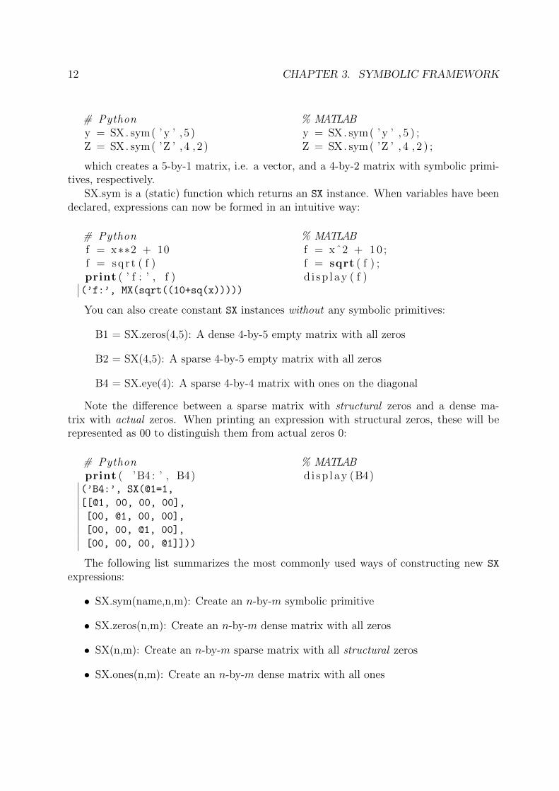
# Pythony = SX. sym( ’ y ’ , 5 )Z = SX. sym( ’Z ’ , 4 , 2 )

% MATLABy = SX. sym( ’ y ’ , 5 ) ;Z = SX. sym( ’Z ’ , 4 , 2 ) ;

which creates a 5-by-1 matrix, i.e. a vector, and a 4-by-2 matrix with symbolic primi-tives, respectively.

SX.sym is a (static) function which returns an SX instance. When variables have beendeclared, expressions can now be formed in an intuitive way:

# Pythonf = x∗∗2 + 10f = s q r t ( f )print ( ’ f : ’ , f )

% MATLABf = xˆ2 + 10 ;f = sqrt ( f ) ;d i sp l ay ( f )

(’f:’, MX(sqrt((10+sq(x)))))

You can also create constant SX instances without any symbolic primitives:

B1 = SX.zeros(4,5): A dense 4-by-5 empty matrix with all zeros

B2 = SX(4,5): A sparse 4-by-5 empty matrix with all zeros

B4 = SX.eye(4): A sparse 4-by-4 matrix with ones on the diagonal

Note the difference between a sparse matrix with structural zeros and a dense ma-trix with actual zeros. When printing an expression with structural zeros, these will berepresented as 00 to distinguish them from actual zeros 0:

# Pythonprint ( ’B4 : ’ , B4)

% MATLABd i sp l ay (B4)

(’B4:’, SX(@1=1,

[[@1, 00, 00, 00],

[00, @1, 00, 00],

[00, 00, @1, 00],

[00, 00, 00, @1]]))

The following list summarizes the most commonly used ways of constructing new SX

expressions:

• SX.sym(name,n,m): Create an n-by-m symbolic primitive

• SX.zeros(n,m): Create an n-by-m dense matrix with all zeros

• SX(n,m): Create an n-by-m sparse matrix with all structural zeros

• SX.ones(n,m): Create an n-by-m dense matrix with all ones

3.1. THE SX SYMBOLICS 13

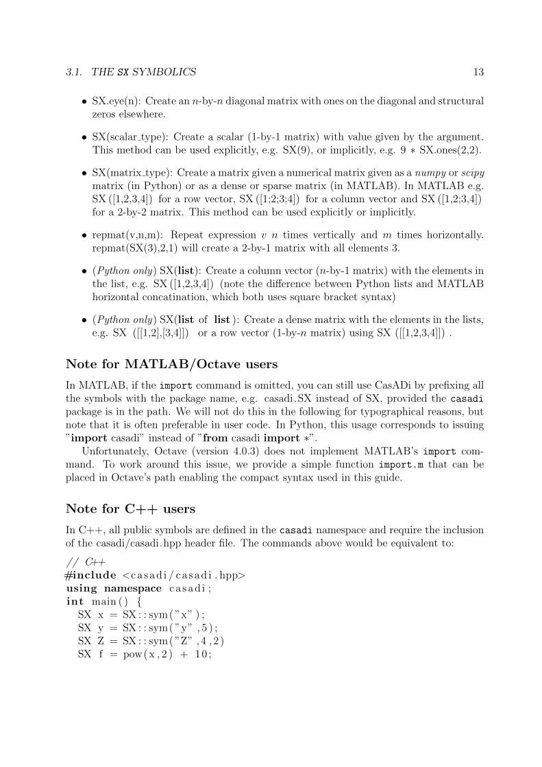
• SX.eye(n): Create an n-by-n diagonal matrix with ones on the diagonal and structuralzeros elsewhere.

• SX(scalar type): Create a scalar (1-by-1 matrix) with value given by the argument.This method can be used explicitly, e.g. SX(9), or implicitly, e.g. 9 ∗ SX.ones(2,2).

• SX(matrix type): Create a matrix given a numerical matrix given as a numpy or scipymatrix (in Python) or as a dense or sparse matrix (in MATLAB). In MATLAB e.g.SX ([1,2,3,4]) for a row vector, SX ([1;2;3;4]) for a column vector and SX ([1,2;3,4])for a 2-by-2 matrix. This method can be used explicitly or implicitly.

• repmat(v,n,m): Repeat expression v n times vertically and m times horizontally.repmat(SX(3),2,1) will create a 2-by-1 matrix with all elements 3.

• (Python only) SX(list): Create a column vector (n-by-1 matrix) with the elements inthe list, e.g. SX ([1,2,3,4]) (note the difference between Python lists and MATLABhorizontal concatination, which both uses square bracket syntax)

• (Python only) SX(list of list ): Create a dense matrix with the elements in the lists,e.g. SX ([[1,2],[3,4]]) or a row vector (1-by-n matrix) using SX ([[1,2,3,4]]) .

Note for MATLAB/Octave users

In MATLAB, if the import command is omitted, you can still use CasADi by prefixing allthe symbols with the package name, e.g. casadi.SX instead of SX, provided the casadi

package is in the path. We will not do this in the following for typographical reasons, butnote that it is often preferable in user code. In Python, this usage corresponds to issuing”import casadi” instead of ”from casadi import ∗”.

Unfortunately, Octave (version 4.0.3) does not implement MATLAB’s import com-mand. To work around this issue, we provide a simple function import.m that can beplaced in Octave’s path enabling the compact syntax used in this guide.

Note for C++ users

In C++, all public symbols are defined in the casadi namespace and require the inclusionof the casadi/casadi.hpp header file. The commands above would be equivalent to:

// C++#include <ca sad i / ca sad i . hpp>using namespace ca sad i ;int main ( ) {

SX x = SX : : sym( ”x” ) ;SX y = SX : : sym( ”y” , 5 ) ;SX Z = SX : : sym( ”Z” ,4 , 2 )SX f = pow(x , 2 ) + 10 ;


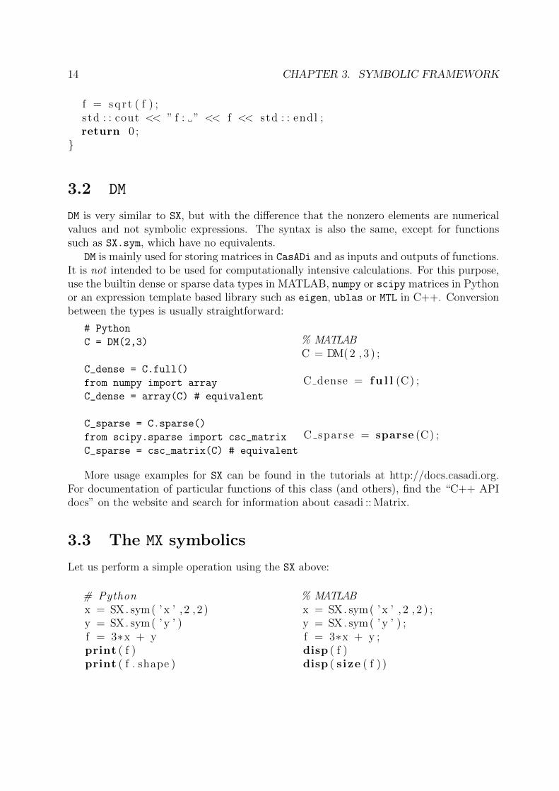
f = s q r t ( f ) ;s td : : cout << ” f : ” << f << std : : endl ;return 0 ;

}

3.2 DM

DM is very similar to SX, but with the difference that the nonzero elements are numericalvalues and not symbolic expressions. The syntax is also the same, except for functionssuch as SX.sym, which have no equivalents.

DM is mainly used for storing matrices in CasADi and as inputs and outputs of functions.It is not intended to be used for computationally intensive calculations. For this purpose,use the builtin dense or sparse data types in MATLAB, numpy or scipy matrices in Pythonor an expression template based library such as eigen, ublas or MTL in C++. Conversionbetween the types is usually straightforward:

# Python

C = DM(2,3)

C_dense = C.full()

from numpy import array

C_dense = array(C) # equivalent

C_sparse = C.sparse()

from scipy.sparse import csc_matrix

C_sparse = csc_matrix(C) # equivalent

% MATLABC = DM( 2 , 3 ) ;

C dense = f u l l (C) ;

C sparse = sparse (C) ;

More usage examples for SX can be found in the tutorials at http://docs.casadi.org.For documentation of particular functions of this class (and others), find the “C++ APIdocs” on the website and search for information about casadi :: Matrix.

3.3 The MX symbolics

Let us perform a simple operation using the SX above:

# Pythonx = SX. sym( ’ x ’ , 2 , 2 )y = SX. sym( ’ y ’ )f = 3∗x + yprint ( f )print ( f . shape )

% MATLABx = SX. sym( ’ x ’ , 2 , 2 ) ;y = SX. sym( ’ y ’ ) ;f = 3∗x + y ;disp ( f )disp ( s ize ( f ) )

http://docs.casadi.org/

3.3. THE MX SYMBOLICS 15

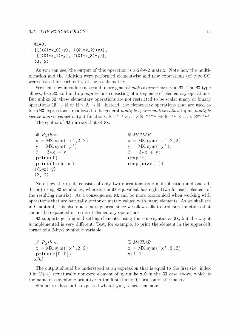
@1=3,

[[((@1*x_0)+y), ((@1*x_2)+y)],

[((@1*x_1)+y), ((@1*x_3)+y)]]

(2, 2)

As you can see, the output of this operation is a 2-by-2 matrix. Note how the multi-plication and the addition were performed elementwise and new expressions (of type SX)were created for each entry of the result matrix.

We shall now introduce a second, more general matrix expression type MX. The MX typeallows, like SX, to build up expressions consisting of a sequence of elementary operations.But unlike SX, these elementary operations are not restricted to be scalar unary or binaryoperations (R → R or R × R → R. Instead, the elementary operations that are used toform MX expressions are allowed to be general multiple sparse-matrix valued input, multiplesparse-matrix valued output functions: Rn1×m1 × . . .×RnN×mN → Rp1×q1 × . . .×RpM×qM .

The syntax of MX mirrors that of SX:

# Pythonx = MX. sym( ’ x ’ , 2 , 2 )y = MX. sym( ’ y ’ )f = 3∗x + yprint ( f )print ( f . shape )

% MATLABx = MX. sym( ’ x ’ , 2 , 2 ) ;y = MX. sym( ’ y ’ ) ;f = 3∗x + y ;disp ( f )disp ( s ize ( f ) )

((3*x)+y)

(2, 2)

Note how the result consists of only two operations (one multiplication and one ad-dition) using MX symbolics, whereas the SX equivalent has eight (two for each element ofthe resulting matrix). As a consequence, MX can be more economical when working withoperations that are naturally vector or matrix valued with many elements. As we shall seein Chapter 4, it is also much more general since we allow calls to arbitrary functions thatcannot be expanded in terms of elementary operations.

MX supports getting and setting elements, using the same syntax as SX, but the way itis implemented is very different. Test, for example, to print the element in the upper-leftcorner of a 2-by-2 symbolic variable:

# Pythonx = MX. sym( ’ x ’ , 2 , 2 )print ( x [ 0 , 0 ] )

% MATLABx = MX. sym( ’ x ’ , 2 , 2 ) ;x (1 , 1 )

x[0]

The output should be understood as an expression that is equal to the first (i.e. index0 in C++) structurally non-zero element of x, unlike x 0 in the SX case above, which isthe name of a symbolic primitive in the first (index 0) location of the matrix.

Similar results can be expected when trying to set elements:


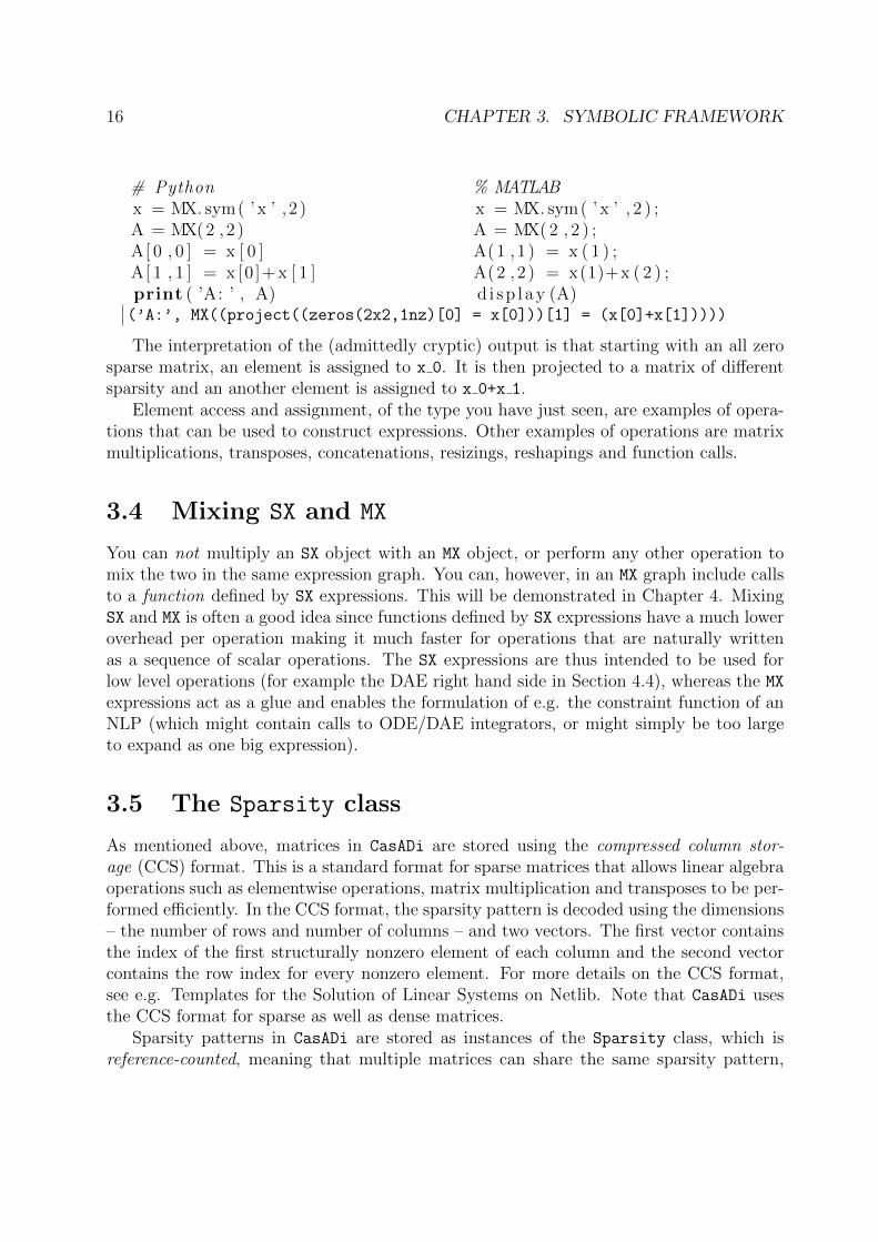
# Pythonx = MX. sym( ’ x ’ , 2 )A = MX(2 ,2 )A[ 0 , 0 ] = x [ 0 ]A[ 1 , 1 ] = x [0 ]+ x [ 1 ]print ( ’A: ’ , A)

% MATLABx = MX. sym( ’ x ’ , 2 ) ;A = MX( 2 , 2 ) ;A(1 , 1 ) = x ( 1 ) ;A(2 , 2 ) = x(1)+x ( 2 ) ;d i sp l ay (A)

(’A:’, MX((project((zeros(2x2,1nz)[0] = x[0]))[1] = (x[0]+x[1]))))

The interpretation of the (admittedly cryptic) output is that starting with an all zerosparse matrix, an element is assigned to x 0. It is then projected to a matrix of differentsparsity and an another element is assigned to x 0+x 1.

Element access and assignment, of the type you have just seen, are examples of opera-tions that can be used to construct expressions. Other examples of operations are matrixmultiplications, transposes, concatenations, resizings, reshapings and function calls.

3.4 Mixing SX and MX

You can not multiply an SX object with an MX object, or perform any other operation tomix the two in the same expression graph. You can, however, in an MX graph include callsto a function defined by SX expressions. This will be demonstrated in Chapter 4. MixingSX and MX is often a good idea since functions defined by SX expressions have a much loweroverhead per operation making it much faster for operations that are naturally writtenas a sequence of scalar operations. The SX expressions are thus intended to be used forlow level operations (for example the DAE right hand side in Section 4.4), whereas the MX

expressions act as a glue and enables the formulation of e.g. the constraint function of anNLP (which might contain calls to ODE/DAE integrators, or might simply be too largeto expand as one big expression).

3.5 The Sparsity class

As mentioned above, matrices in CasADi are stored using the compressed column stor-age (CCS) format. This is a standard format for sparse matrices that allows linear algebraoperations such as elementwise operations, matrix multiplication and transposes to be per-formed efficiently. In the CCS format, the sparsity pattern is decoded using the dimensions– the number of rows and number of columns – and two vectors. The first vector containsthe index of the first structurally nonzero element of each column and the second vectorcontains the row index for every nonzero element. For more details on the CCS format,see e.g. Templates for the Solution of Linear Systems on Netlib. Note that CasADi usesthe CCS format for sparse as well as dense matrices.

Sparsity patterns in CasADi are stored as instances of the Sparsity class, which isreference-counted, meaning that multiple matrices can share the same sparsity pattern,

http://netlib.org/linalg/html_templates/node92.html

3.5. THE SPARSITY CLASS 17

including MX expression graphs and instances of SX and DM. The Sparsity class is alsocached, meaning that the creation of multiple instances of the same sparsity patterns isalways avoided.

The following list summarizes the most commonly used ways of constructing new spar-sity patterns:

• Sparsity.dense(n,m): Create a dense n-by-m sparsity pattern

• Sparsity(n,m): Create a sparse n-by-m sparsity pattern

• Sparsity.diag(n): Create a diagonal n-by-n sparsity pattern

• Sparsity.upper(n): Create an upper triangular n-by-n sparsity pattern

• Sparsity.lower(n): Create a lower triangular n-by-n sparsity pattern

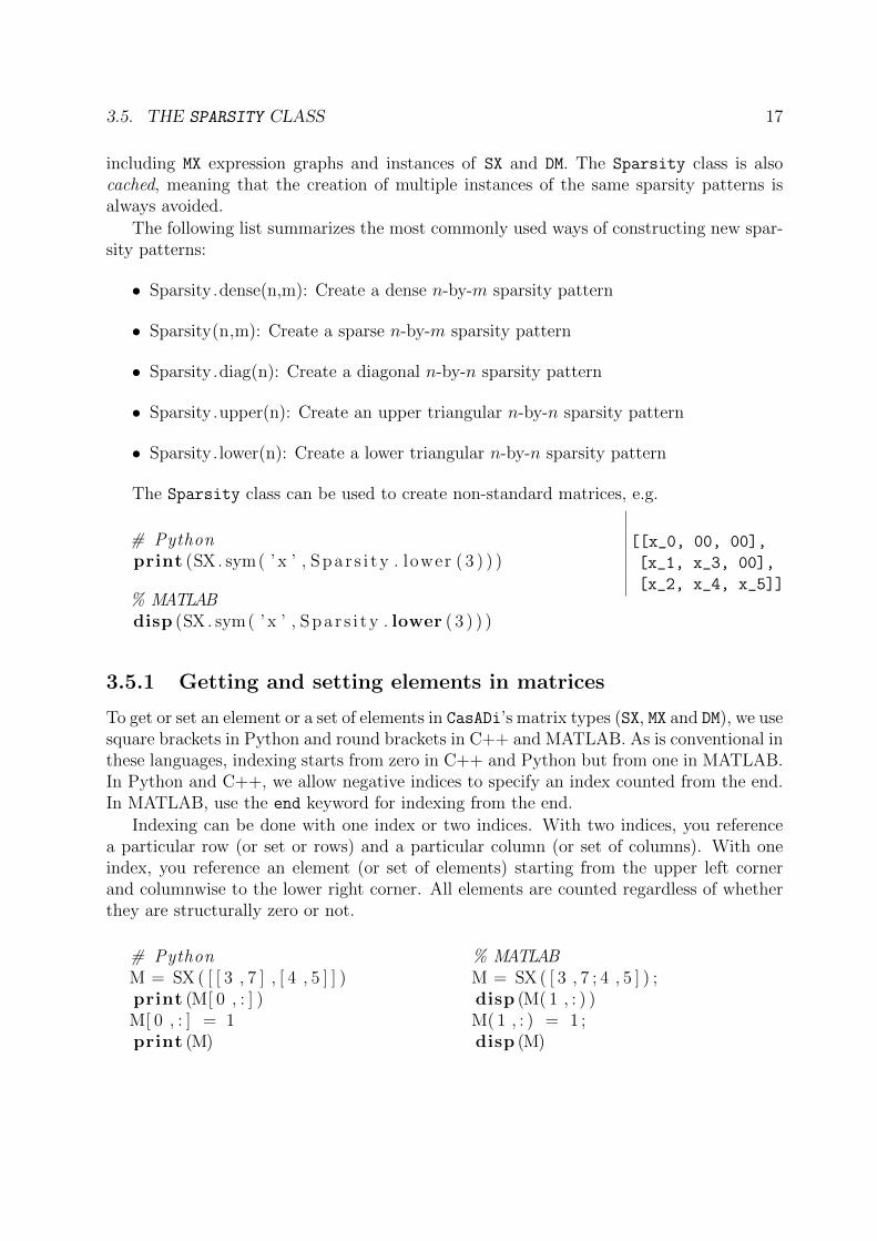
The Sparsity class can be used to create non-standard matrices, e.g.

# Pythonprint (SX. sym( ’ x ’ , Spa r s i t y . lower ( 3 ) ) )

% MATLABdisp (SX. sym( ’ x ’ , Spa r s i ty . lower ( 3 ) ) )

[[x_0, 00, 00],

[x_1, x_3, 00],

[x_2, x_4, x_5]]

3.5.1 Getting and setting elements in matrices

To get or set an element or a set of elements in CasADi’s matrix types (SX, MX and DM), we usesquare brackets in Python and round brackets in C++ and MATLAB. As is conventional inthese languages, indexing starts from zero in C++ and Python but from one in MATLAB.In Python and C++, we allow negative indices to specify an index counted from the end.In MATLAB, use the end keyword for indexing from the end.

Indexing can be done with one index or two indices. With two indices, you referencea particular row (or set or rows) and a particular column (or set of columns). With oneindex, you reference an element (or set of elements) starting from the upper left cornerand columnwise to the lower right corner. All elements are counted regardless of whetherthey are structurally zero or not.

# PythonM = SX ( [ [ 3 , 7 ] , [ 4 , 5 ] ] )print (M[ 0 , : ] )M[ 0 , : ] = 1print (M)

% MATLABM = SX ( [ 3 , 7 ; 4 , 5 ] ) ;disp (M( 1 , : ) )M( 1 , : ) = 1 ;disp (M)


[[3, 7]]

@1=1,

[[@1, @1],

[4, 5]]

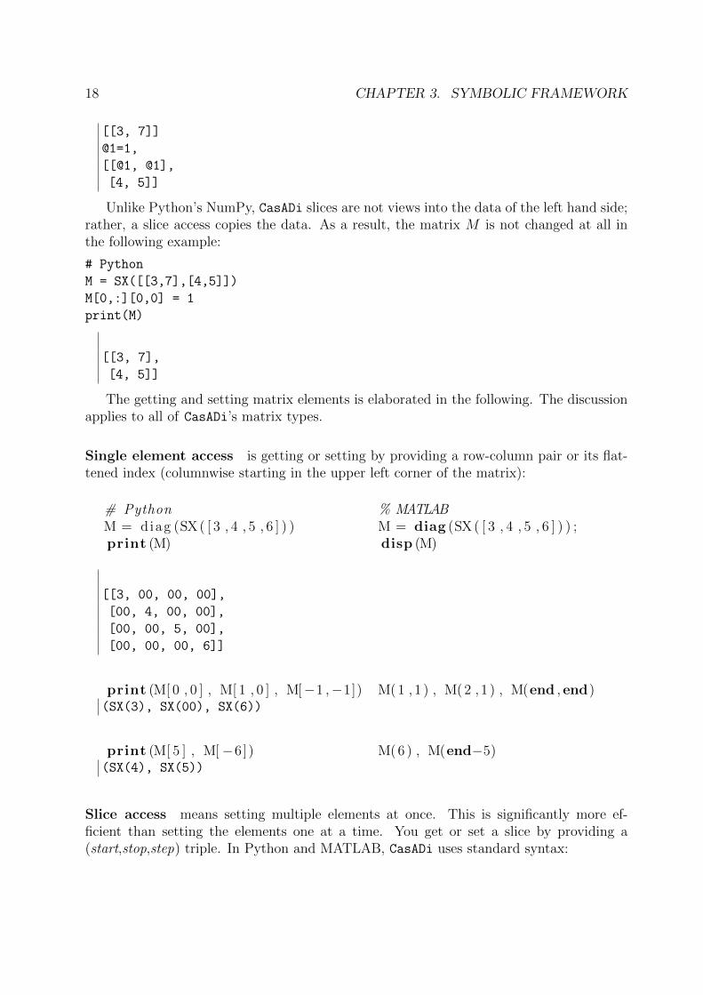
Unlike Python’s NumPy, CasADi slices are not views into the data of the left hand side;rather, a slice access copies the data. As a result, the matrix M is not changed at all inthe following example:

# Python

M = SX([[3,7],[4,5]])

M[0,:][0,0] = 1

print(M)

[[3, 7],

[4, 5]]

The getting and setting matrix elements is elaborated in the following. The discussionapplies to all of CasADi’s matrix types.

Single element access is getting or setting by providing a row-column pair or its flat-tened index (columnwise starting in the upper left corner of the matrix):

# PythonM = diag (SX( [ 3 , 4 , 5 , 6 ] ) )print (M)

% MATLABM = diag (SX( [ 3 , 4 , 5 , 6 ] ) ) ;disp (M)

[[3, 00, 00, 00],

[00, 4, 00, 00],

[00, 00, 5, 00],

[00, 00, 00, 6]]

print (M[ 0 , 0 ] , M[ 1 , 0 ] , M[−1 ,−1]) M( 1 , 1 ) , M( 2 , 1 ) , M(end , end)(SX(3), SX(00), SX(6))

print (M[ 5 ] , M[−6]) M( 6 ) , M(end−5)(SX(4), SX(5))

Slice access means setting multiple elements at once. This is significantly more ef-ficient than setting the elements one at a time. You get or set a slice by providing a(start,stop,step) triple. In Python and MATLAB, CasADi uses standard syntax:

3.6. ARITHMETIC OPERATIONS 19

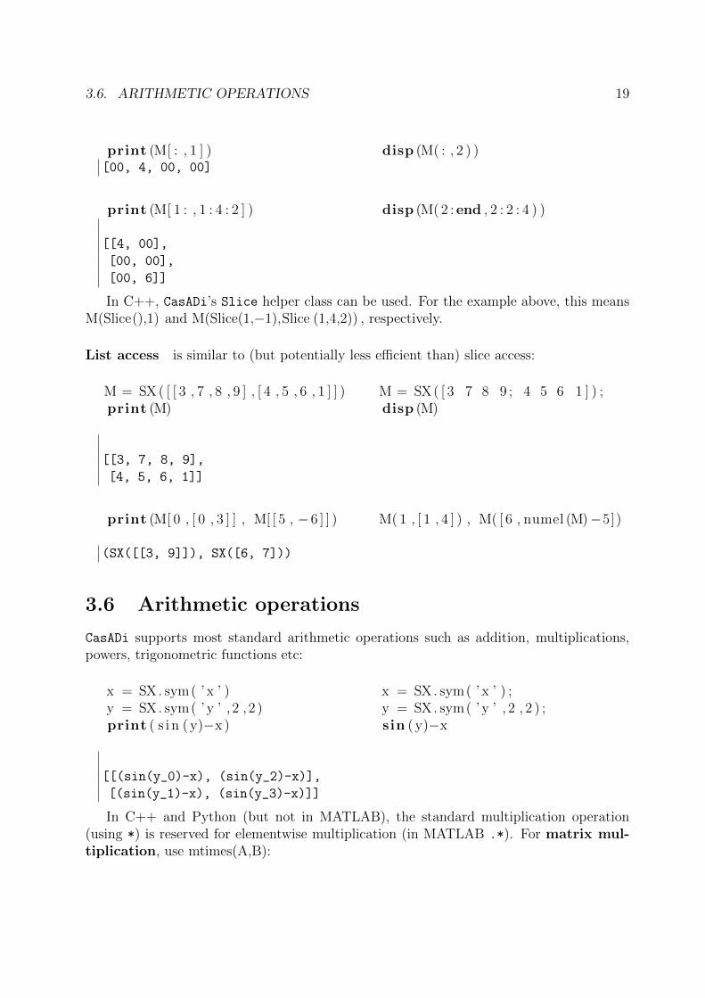
print (M[ : , 1 ] ) disp (M( : , 2 ) )[00, 4, 00, 00]

print (M[ 1 : , 1 : 4 : 2 ] ) disp (M( 2 : end , 2 : 2 : 4 ) )

[[4, 00],

[00, 00],

[00, 6]]

In C++, CasADi’s Slice helper class can be used. For the example above, this meansM(Slice(),1) and M(Slice(1,−1),Slice (1,4,2)) , respectively.

List access is similar to (but potentially less efficient than) slice access:

M = SX ( [ [ 3 , 7 , 8 , 9 ] , [ 4 , 5 , 6 , 1 ] ] )print (M)

M = SX( [ 3 7 8 9 ; 4 5 6 1 ] ) ;disp (M)

[[3, 7, 8, 9],

[4, 5, 6, 1]]

print (M[ 0 , [ 0 , 3 ] ] , M[ [ 5 , − 6 ] ] ) M( 1 , [ 1 , 4 ] ) , M( [ 6 , numel (M)−5])

(SX([[3, 9]]), SX([6, 7]))

3.6 Arithmetic operations

CasADi supports most standard arithmetic operations such as addition, multiplications,powers, trigonometric functions etc:

x = SX. sym( ’ x ’ )y = SX. sym( ’ y ’ , 2 , 2 )print ( s i n ( y)−x )

x = SX. sym( ’ x ’ ) ;y = SX. sym( ’ y ’ , 2 , 2 ) ;sin ( y)−x

[[(sin(y_0)-x), (sin(y_2)-x)],

[(sin(y_1)-x), (sin(y_3)-x)]]

In C++ and Python (but not in MATLAB), the standard multiplication operation(using *) is reserved for elementwise multiplication (in MATLAB .*). For matrix mul-tiplication, use mtimes(A,B):


print ( y∗y , mtimes (y , y ) ) y .∗ y , y∗y

(SX(

[[sq(y_0), sq(y_2)],

[sq(y_1), sq(y_3)]]), SX(

[[(sq(y_0)+(y_2*y_1)), ((y_0*y_2)+(y_2*y_3))],

[((y_1*y_0)+(y_3*y_1)), ((y_1*y_2)+sq(y_3))]]))

As is customary in MATLAB, multiplication using * and .* are equivalent when eitherof the arguments is a scalar.

Transposes are formed using the syntax A.T in Python, A.T() in C++ and with A’or A.’ in MATLAB:

print ( y .T) y ’

[[y_0, y_1],

[y_2, y_3]]

Reshaping means changing the number of rows and columns but retaining the numberof elements and the relative location of the nonzeros. This is a computationally very cheapoperation which is performed using the syntax:

x = SX. eye (4 )print ( reshape (x , 2 , 8 ) )

x = SX. eye ( 4 ) ;reshape (x , 2 , 8 )

@1=1,

[[@1, 00, 00, 00, 00, @1, 00, 00],

[00, 00, @1, 00, 00, 00, 00, @1]]

Concatenation means stacking matrices horizontally or vertically. Due to the column-major way of storing elements in CasADi, it is most efficient to stack matrices horizontally.Matrices that are in fact column vectors (i.e. consisting of a single column), can also bestacked efficiently vertically. Vertical and horizontal concatenation is performed using thefunctions vertcat and horzcat (that take a list of input arguments) in Python and C++and with square brackets in MATLAB:

x = SX. sym( ’ x ’ , 5 )y = SX. sym( ’ y ’ , 5 )print ( v e r t c a t (x , y ) )

x = SX. sym( ’ x ’ , 5 ) ;y = SX. sym( ’ y ’ , 5 ) ;[ x ; y ]

[x_0, x_1, x_2, x_3, x_4, y_0, y_1, y_2, y_3, y_4]

3.6. ARITHMETIC OPERATIONS 21

print ( horzcat (x , y ) ) [ x , y ]

[[x_0, y_0],

[x_1, y_1],

[x_2, y_2],

[x_3, y_3],

[x_4, y_4]]

Horizontal and vertical splitting are the inverse operations of the above introducedhorizontal and vertical concatenation. To split up an expression horizontally into n smallerexpressions, you need to provide, in addition to the expression being splitted, a vectoroffset of length n + 1. The first element of the offset vector must be 0 and the lastelement must be the number of columns. Remaining elements must follow in a non-decreasing order. The output i of the splitting operation then contains the columns c withoffset[i] ≤ c < offset[i+ 1]. The following demonstrates the syntax:

x = SX. sym( ’ x ’ , 5 , 2 )w = h o r z s p l i t (x , [ 0 , 1 , 2 ] )print (w[ 0 ] , w [ 1 ] )

x = SX. sym( ’ x ’ , 5 , 2 ) ;w = h o r z s p l i t (x , [ 0 , 1 , 2 ] ) ;w{1} , w{2}

(SX([x_0, x_1, x_2, x_3, x_4]), SX([x_5, x_6, x_7, x_8, x_9]))

The vertsplit operation works analogously, but with the offset vector referring to rows:

w = v e r t s p l i t (x , [ 0 , 3 , 5 ] )print (w[ 0 ] , w [ 1 ] )

w = v e r t s p l i t (x , [ 0 , 3 , 5 ] ) ;w{1} , w{2}

(SX(

[[x_0, x_5],

[x_1, x_6],

[x_2, x_7]]), SX(

[[x_3, x_8],

[x_4, x_9]]))

Note that it is always possible to use slice element access instead of horizontal andvertical splitting, for the above vertical splitting:

w = [ x [ 0 : 3 , : ] , x [ 3 : 5 , : ] ]print (w[ 0 ] , w [ 1 ] )

w = {x ( 1 : 3 , : ) , x ( 4 : 5 , : ) } ;w{1} , w{2}

(SX(

[[x_0, x_5],


[x_1, x_6],

[x_2, x_7]]), SX(

[[x_3, x_8],

[x_4, x_9]]))

For SX graphs, this alternative way is completely equivalent, but for MX graphs usinghorzsplit/vertsplit is significantly more efficient when all the splitted expressions areneeded.

Inner product, defined as < A,B >:= tr(AB) =∑

i,j Ai,j Bi,j are created as follows:

x = SX. sym( ’ x ’ , 2 , 2 )print ( dot (x , x ) )

x = SX. sym( ’ x ’ , 2 , 2 )dot (x , x )

(((sq(x_0)+sq(x_1))+sq(x_2))+sq(x_3))

Many of the above operations are also defined for the Sparsity class (Section 3.5),e.g. vertcat, horzsplit, transposing, addition (which returns the union of two sparsitypatterns) and multiplication (which returns the intersection of two sparsity patterns).

3.7 Querying properties

You can check if a matrix or sparsity pattern has a certain property by calling an appro-priate member function. e.g.

y = SX. sym( ’ y ’ , 10 ,1 )print ( y . shape )

y = SX. sym( ’ y ’ , 1 0 , 1 ) ;s ize ( y )

(10, 1)

Note that in MATLAB, obj.myfcn(arg) and myfcn(obj, arg) are both valid ways ofcalling a member function myfcn. The latter variant is probably preferable from a styleviewpoint.

Some commonly used properties for a matrix A are:

A.size1() The number of rows

A.size2() The number of columns

A.shape (in MATLAB ”size”) The shape, i.e. the pair (nrow,ncol)

A.numel() The number of elements, i.e nrow ∗ ncol

A.nnz() The number of structurally nonzero elements, equal to A.numel() if dense.

A.sparsity() Retrieve a reference to the sparsity pattern

3.8. LINEAR ALGEBRA 23

A.is dense() Is a matrix dense, i.e. having no structural zeros

A.is scalar() Is the matrix a scalar, i.e. having dimensions 1-by-1?

A.is column() Is the matrix a vector, i.e. having dimensions n-by-1?

A.is square() Is the matrix square?

A.is triu() Is the matrix upper triangular?

A.is constant() Are the matrix entries all constant?

A.is integer() Are the matrix entries all integer-valued?

The last queries are examples of queries for which false negative returns are allowed.A matrix for which A.is constant() is true is guaranteed to be constant, but is not guar-anteed to be non-constant if A.is constant() is false. We recommend you to check the APIdocumentation for a particular function before using it for the first time.

3.8 Linear algebra

CasADi supports a limited number of linear algebra operations, e.g. for solution of linearsystems of equations:

A = MX. sym( ’A ’ , 3 , 3 )b = MX. sym( ’b ’ , 3 )print ( s o l v e (A, b ) )

A = MX. sym( ’A ’ , 3 , 3 ) ;b = MX. sym( ’b ’ , 3 ) ;s o l v e (A, b)

(A\b)

3.9 Calculus – algorithmic differentiation

The single most central functionality of CasADi is algorithmic (or automatic) differentiation(AD). For a function f : RN → RM :

y = f(x), (3.1)

Forward mode directional derivatives can be used to calculate Jacobian-times-vector prod-ucts:

y =∂f

∂xx. (3.2)

Similarly, reverse mode directional derivatives can be used to calculate Jacobian-transposed-times-vector products:

x =

(∂f

∂x

)T

y. (3.3)


Both forward and reverse mode directional derivatives are calculated at a cost propor-tional to evaluating f(x), regardless of the dimension of x.

CasADi is also able to generate complete, sparse Jacobians efficiently. The algorithmfor this is very complex, but essentially consists of the following steps:

• Automatically detect the sparsity pattern of the Jacobian

• Use graph coloring techniques to find a few forward and/or directional derivativesneeded to construct the complete Jacobian

• Calculate the directional derivatives numerically or symbolically

• Assemble the complete Jacobian

Hessians are calculated by first calculating the gradient and then performing the samesteps as above to calculate the Jacobian of the gradient in the same way as above, whileexploiting symmetry.

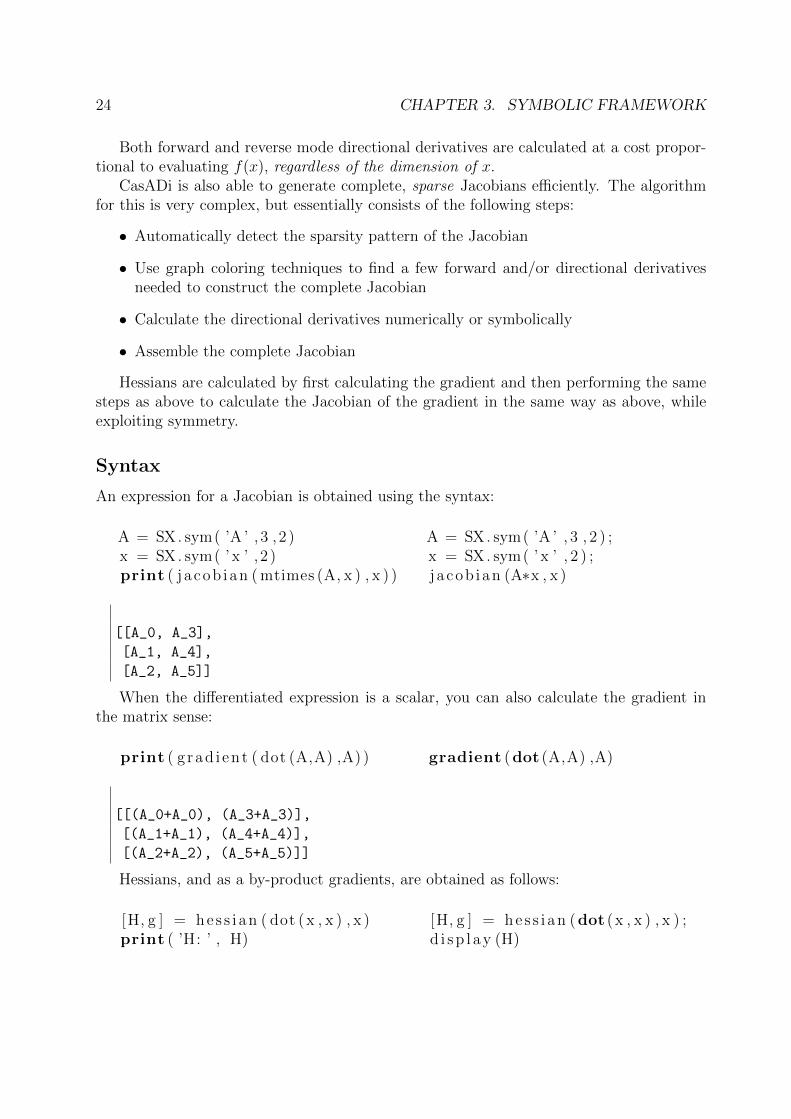
Syntax

An expression for a Jacobian is obtained using the syntax:

A = SX. sym( ’A ’ , 3 , 2 )x = SX. sym( ’ x ’ , 2 )print ( j acob ian ( mtimes (A, x ) , x ) )

A = SX. sym( ’A ’ , 3 , 2 ) ;x = SX. sym( ’ x ’ , 2 ) ;j a cob ian (A∗x , x )

[[A_0, A_3],

[A_1, A_4],

[A_2, A_5]]

When the differentiated expression is a scalar, you can also calculate the gradient inthe matrix sense:

print ( g rad i en t ( dot (A,A) ,A) ) gradient (dot (A,A) ,A)

[[(A_0+A_0), (A_3+A_3)],

[(A_1+A_1), (A_4+A_4)],

[(A_2+A_2), (A_5+A_5)]]

Hessians, and as a by-product gradients, are obtained as follows:

[H, g ] = he s s i an ( dot (x , x ) , x )print ( ’H: ’ , H)

[H, g ] = hes s i an (dot (x , x ) , x ) ;d i sp l ay (H)

3.9. CALCULUS – ALGORITHMIC DIFFERENTIATION 25

(’H:’, SX(@1=2,

[[@1, 00],

[00, @1]]))

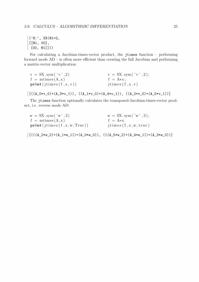
For calculating a Jacobian-times-vector product, the jtimes function – performingforward mode AD – is often more efficient than creating the full Jacobian and performinga matrix-vector multiplication:

v = SX. sym( ’ v ’ , 2 )f = mtimes (A, x )print ( j t imes ( f , x , v ) )

v = SX. sym( ’ v ’ , 2 ) ;f = A∗x ;j t imes ( f , x , v )

[((A_0*v_0)+(A_3*v_1)), ((A_1*v_0)+(A_4*v_1)), ((A_2*v_0)+(A_5*v_1))]

The jtimes function optionally calculates the transposed-Jacobian-times-vector prod-uct, i.e. reverse mode AD:

w = SX. sym( ’w ’ ,3 )f = mtimes (A, x )print ( j t imes ( f , x ,w, True ) )

w = SX. sym( ’w ’ , 3 ) ;f = A∗xj t imes ( f , x ,w, t rue )

[(((A_2*w_2)+(A_1*w_1))+(A_0*w_0)), (((A_5*w_2)+(A_4*w_1))+(A_3*w_0))]


Chapter 4

Function objects

CasADi allows the user to create function objects, in C++ terminology often referred toas functors. This includes functions that are defined by a symbolic expression, ODE/DAEintegrators, QP solvers, NLP solvers etc.

Function objects are typically created with the syntax:

f = functionname (name , arguments , . . . , [ opt ions ] )

The name is mainly a display name that will show up in e.g. error messages or ascomments in generated C code. This is followed by a set of arguments, which is classdependent. Finally, the user can pass an options structure for customizing the behavior ofthe class. The options structure is a dictionary type in Python, a struct in MATLAB orCasADi’s Dict type in C++.

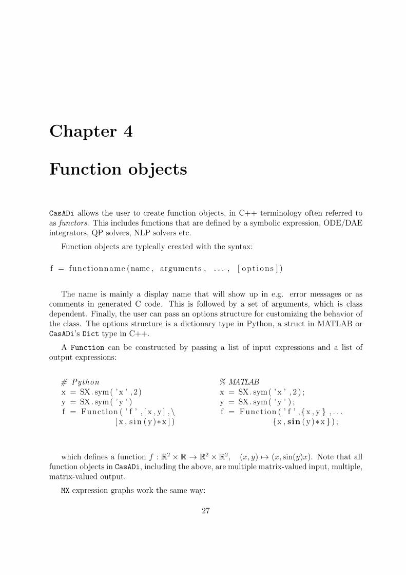
A Function can be constructed by passing a list of input expressions and a list ofoutput expressions:

# Pythonx = SX. sym( ’ x ’ , 2 )y = SX. sym( ’ y ’ )f = Function ( ’ f ’ , [ x , y ] ,\

[ x , s i n ( y )∗x ] )

% MATLABx = SX. sym( ’ x ’ , 2 ) ;y = SX. sym( ’ y ’ ) ;f = Function ( ’ f ’ ,{x , y } , . . .

{x , sin ( y )∗x } ) ;

which defines a function f : R2 × R → R2 × R2, (x, y) 7→ (x, sin(y)x). Note that allfunction objects in CasADi, including the above, are multiple matrix-valued input, multiple,matrix-valued output.

MX expression graphs work the same way:

27

28 CHAPTER 4. FUNCTION OBJECTS

# Pythonx = MX. sym( ’ x ’ , 2 )y = MX. sym( ’ y ’ )f = Function ( ’ f ’ , [ x , y ] ,\

[ x , s i n ( y )∗x ] )

% MATLABx = MX. sym( ’ x ’ , 2 ) ;y = MX. sym( ’ y ’ ) ;f = Function ( ’ f ’ ,{x , y } , . . .

{x , sin ( y )∗x } ) ;

When creating a Function from expressions like that, it is always advisory to namethe inputs and outputs as follows:


[ x , s i n ( y )∗x ] ,\[ ’ x ’ , ’ y ’ ] , [ ’ r ’ , ’ q ’ ] )


{x , sin ( y )∗x } , . . .{ ’ x ’ , ’ y ’ } ,{ ’ r ’ , ’ q ’ } ) ;

Naming inputs and outputs is preferred for a number of reasons:

• No need to remember the number or order of arguments

• Inputs or outputs that are absent can be left unset

• More readable and less error prone syntax. E.g. f.jacobian(’x’,’q’) instead off.jacobian(0,1).

For Function instances – to be encountered later – that are not created directly fromexpressions, the inputs and outputs are named automatically.

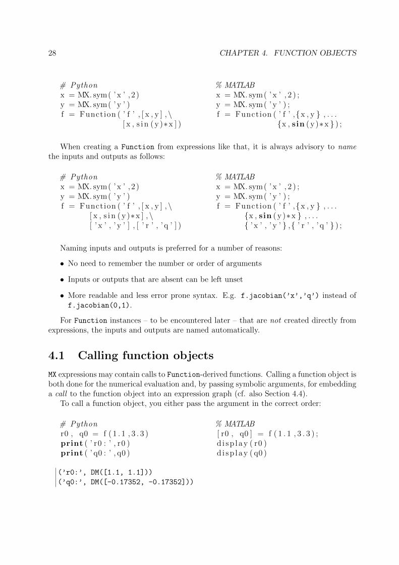
4.1 Calling function objects

MX expressions may contain calls to Function-derived functions. Calling a function object isboth done for the numerical evaluation and, by passing symbolic arguments, for embeddinga call to the function object into an expression graph (cf. also Section 4.4).

To call a function object, you either pass the argument in the correct order:

# Pythonr0 , q0 = f ( 1 . 1 , 3 . 3 )print ( ’ r0 : ’ , r0 )print ( ’ q0 : ’ , q0 )

% MATLAB[ r0 , q0 ] = f ( 1 . 1 , 3 . 3 ) ;d i sp l ay ( r0 )d i sp l ay ( q0 )

(’r0:’, DM([1.1, 1.1]))

(’q0:’, DM([-0.17352, -0.17352]))

4.2. CONVERTING MX TO SX 29

or the arguments and their names as follows, which will result in a dictionary (dict inPython, struct in MATLAB and std :: map<std::string, MatrixType> in C++):

# Pythonr e s = f ( x=1.1 , y=3.3)print ( ’ r e s : ’ , r e s )

% MATLABr e s = f ( ’ x ’ , 1 . 1 , ’ y ’ , 3 . 3 ) ;d i sp l ay ( r e s )

(’res:’, {’q’: DM([-0.17352, -0.17352]), ’r’: DM([1.1, 1.1])})

When calling a function object, the dimensions (but not necessarily the sparsity pat-terns) of the evaluation arguments have to match those of the function inputs, with twoexceptions:

• A row vector can be passed instead of a column vector and vice versa.

• A scalar argument can always be passed, regardless of the input dimension. This hasthe meaning of setting all elements of the input matrix to that value.

When the number of inputs to a function object is large or changing, an alternativesyntax to the above is to use the call function which takes a Python list / MATLAB cellarray or, alternatively, a Python dict / MATLAB struct. The return value will have thesame type:

# Pythonarg = [ 1 . 1 , 3 . 3 ]r e s = f . c a l l ( arg )print ( ’ r e s : ’ , r e s )arg = { ’ x ’ : 1 . 1 , ’ y ’ : 3 . 3 }r e s = f . c a l l ( arg )print ( ’ r e s : ’ , r e s )

% MATLABarg = { 1 . 1 , 3 . 3 } ;r e s = f . c a l l ( arg ) ;d i sp l ay ( r e s )arg = s t r u c t ( ’ x ’ , 1 . 1 , ’ y ’ , 3 . 3 ) ;r e s = f . c a l l ( arg ) ;d i sp l ay ( r e s )

(’res:’, [DM([1.1, 1.1]), DM([-0.17352, -0.17352])])

(’res:’, {’q’: DM([-0.17352, -0.17352]), ’r’: DM([1.1, 1.1])})

4.2 Converting MX to SX

A function object defined by an MX graph that only contains built-in operations (e.g.elementwise operations such as addition, square root, matrix multiplications and calls toSX functions, can be converted into a function defined purely by an SX graph using thesyntax:

s x f u n c t i o n = mx function . expand ( )

This might speed up the calculations significantly, but might also cause extra memoryoverhead.


4.3 Nonlinear root-finding problems

Consider the following system of equations:

g0(z, x1, x2, . . . , xn) = 0

g1(z, x1, x2, . . . , xn) = y1

g2(z, x1, x2, . . . , xn) = y2

...

gm(z, x1, x2, . . . , xn) = ym,

(4.1)

where the first equation uniquely defines z as a function of x1, . . . , xn by the implicitfunction theorem and the remaining equations define the auxiliary outputs y1, . . . , ym.

Given a function g for evaluating g0, . . . , gm, we can use CasADi to automatically for-mulate a function G : {zguess, x1, x2, . . . , xn} → {z, y1, y2, . . . , ym}. This function includesa guess for z to handle the case when the solution is non-unique. The syntax for this,assuming n = m = 1 for simplicity, is:

# Pythonz = SX. sym( ’ x ’ , nz )x = SX. sym( ’ x ’ , nx )g0 = ( an expr e s s i on o f x , z )g1 = ( an expr e s s i on o f x , z )g = Function ( ’ g ’ , [ z , x ] , [ g0 , g1 ] )G = r o o t f i n d e r ( ’G’ , ’ newton ’ , g )

% MATLABz = SX. sym( ’ x ’ , nz ) ;x = SX. sym( ’ x ’ , nx ) ;g0 = ( an expr e s s i on o f x , z )g1 = ( an expr e s s i on o f x , z )g = Function ( ’ g ’ ,{ z , x} ,{ g0 , g1 } ) ;G = r o o t f i n d e r ( ’G’ , ’ newton ’ , g ) ;

where the rootfinder function expects a display name, the name of a solver plugin(here a simple full-step Newton method) and the residual function.

Rootfinding objects in CasADi are differential objects and derivatives can be calculatedexactly to arbitrary order.

4.4 Initial-value problems and sensitivity analysis

CasADi can be used to solve initial-value problems in ODE or DAE. The problem formu-lation used is a DAE of semi-explicit form with quadratures:

x = fode(t, x, z, p), x(0) = x0 (4.2a)

0 = falg(t, x, z, p) (4.2b)

q = fquad(t, x, z, p), q(0) = 0 (4.2c)

For solvers of ordinary differential equations, the second equation and the algebraicvariables z must be absent.

4.4. INITIAL-VALUE PROBLEMS AND SENSITIVITY ANALYSIS 31

An integrator in CasADi is a function that takes the state at the initial time x0, a set ofparameters p, and a guess for the algebraic variables (only for DAEs) z0 and returns thestate vector xf, algebraic variables zf and the quadrature state qf, all at the final time.

The freely available SUNDIALS suite (distributed along with CasADi) contains the twopopular integrators CVodes and IDAS for ODEs and DAEs respectively. These integratorshave support for forward and adjoint sensitivity analysis and when used via CasADi’sSundials interface, CasADi will automatically formulate the Jacobian information, which isneeded by the backward differentiation formula (BDF) that CVodes and IDAS use. Alsoautomatically formulated will be the forward and adjoint sensitivity equations.

4.4.1 Creating integrators

Integrators are created using CasADi’s integrator function. Different integrators schemesand interfaces are implemented as plugins, essentially shared libraries that are loaded atruntime.

Consider for example the DAE:

x = z + p, (4.3a)

0 = z cos(z)− x (4.3b)

An integrator, using the ”idas” plugin, can be created using the syntax:

# Pythonx = SX. sym( ’ x ’ ) ; z = SX. sym( ’ z ’ ) ; p = SX. sym( ’p ’ )dae = { ’ x ’ : x , ’ z ’ : z , ’ p ’ : p , ’ ode ’ : z+p , ’ a l g ’ : z∗ cos ( z)−x}F = i n t e g r a t o r ( ’F ’ , ’ i da s ’ , dae )

% MATLABx = SX. sym( ’ x ’ ) ; z = SX. sym( ’ z ’ ) ; p = SX. sym( ’p ’ ) ;dae = s t r u c t ( ’ x ’ , x , ’ z ’ , z , ’ p ’ ,p , ’ ode ’ , z+p , ’ a l g ’ , z∗cos ( z)−x ) ;F = i n t e g r a t o r ( ’F ’ , ’ i da s ’ , dae ) ;

Integrating this DAE from 0 to 1 with x(0) = 0, p = 0.1 and using the guess z(0) = 0,can be done by evaluating the created function object:

# Pythonr = F( x0=0, z0=0, p=0.1)print ( r [ ’ x f ’ ] )

% MATLABr = F( ’ x0 ’ ,0 , ’ z0 ’ , 0 , ’p ’ , 0 . 1 ) ;disp ( r . x f )

0.1724

The time horizon is assumed to be fixed1 and can be changed from its default [0, 1] bysetting the options ”t0” and ”tf”.

1for problems with free end time, you can always scale time by introducing an extra parameter andsubstitute t for a dimensionless time variable that goes from 0 to 1

https://computation.llnl.gov/casc/sundials/description/description.html


4.4.2 Sensitivity analysis

From a usage point of view, an integrator behaves just like the function objects createdfrom expressions earlier in the chapter. You can use member functions in the Functionclass to generate new function objects corresponding to directional derivatives (forward orreverse mode) or complete Jacobians. Then evaluate these function objects numericallyto obtain sensitivity information. The documented example ”sensitivity analysis” (avail-able in CasADi’s example collection for Python, MATLAB and C++) demonstrate howCasADi can be used to calculate first and second order derivative information (forward-over-forward, forward-over-adjoint, adjoint-over-adjoint) for a simple DAE.

4.5 Nonlinear programming

The NLP solvers distributed with or interfaced to CasADi solves parametric NLPs of thefollowing form:

minimize:x

f(x, p)

subject to:xlb ≤ x ≤ xub

glb ≤ g(x, p) ≤ gub

(4.4)

where x ∈ Rnx is the decision variable and p ∈ Rnp is a known parameter vector.An NLP solver in CasADi is a function that takes the parameter value (p), the bounds

(lbx, ubx, lbg, ubg) and a guess for the primal-dual solution (x0, lam x0, lam g0) andreturns the optimal solution. Unlike integrator objects, NLP solver functions are currentlynot differentiable functions in CasADi.

There are several NLP solvers interfaced with CasADi. The most popular one is IPOPT,an open-source primal-dual interior point method which is included in CasADi installations.Others, that require the installation of third-party software, include SNOPT, WORHP andKNITRO. Whatever the NLP solver used, the interface will automatically generate theinformation that it needs to solve the NLP, which may be solver and option dependent.Typically an NLP solver will need a function that gives the Jacobian of the constraintfunction and a Hessian of the Lagrangian function (L(x, λ) = f(x) +λT g(x)) with respectto x.

4.5.1 Creating NLP solvers

NLP solvers are created using CasADi’s nlpsol function. Different solvers and interfacesare implemented as plugins. Consider the following form of the so-called Rosenbrock prob-lem:

minimize:x, y, z

x2 + 100 z2

subject to: z + (1− x)2 − y = 0(4.5)

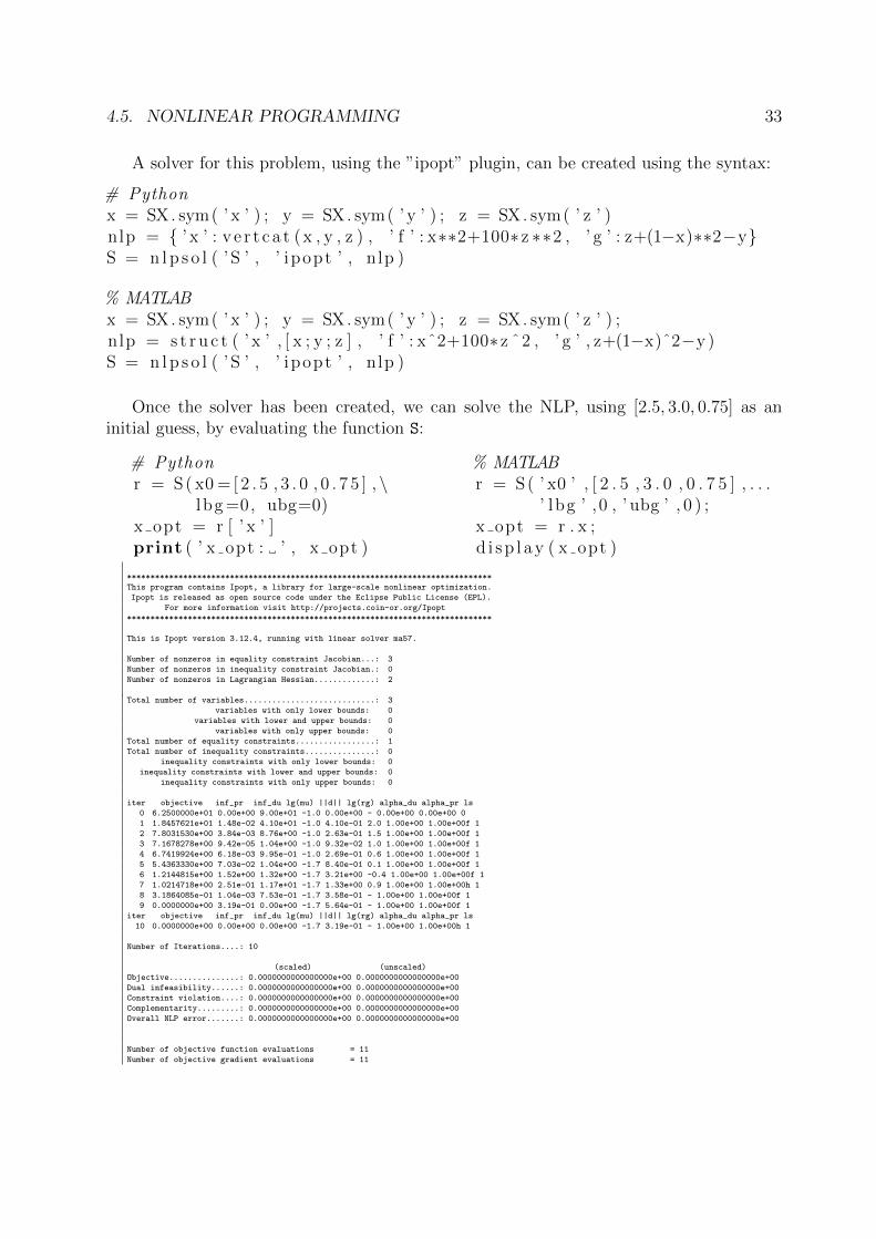
4.5. NONLINEAR PROGRAMMING 33

A solver for this problem, using the ”ipopt” plugin, can be created using the syntax:

# Pythonx = SX. sym( ’ x ’ ) ; y = SX. sym( ’ y ’ ) ; z = SX. sym( ’ z ’ )nlp = { ’ x ’ : v e r t c a t (x , y , z ) , ’ f ’ : x∗∗2+100∗z ∗∗2 , ’ g ’ : z+(1−x)∗∗2−y}S = n l p s o l ( ’S ’ , ’ ipopt ’ , nlp )

% MATLABx = SX. sym( ’ x ’ ) ; y = SX. sym( ’ y ’ ) ; z = SX. sym( ’ z ’ ) ;nlp = s t r u c t ( ’ x ’ , [ x ; y ; z ] , ’ f ’ : xˆ2+100∗z ˆ2 , ’ g ’ , z+(1−x)ˆ2−y )S = n l p s o l ( ’S ’ , ’ ipopt ’ , nlp )

Once the solver has been created, we can solve the NLP, using [2.5, 3.0, 0.75] as aninitial guess, by evaluating the function S:

# Pythonr = S( x0 = [ 2 . 5 , 3 . 0 , 0 . 7 5 ] ,\

lbg =0, ubg=0)x opt = r [ ’ x ’ ]print ( ’ x opt : ’ , x opt )

% MATLABr = S( ’ x0 ’ , [ 2 . 5 , 3 . 0 , 0 . 7 5 ] , . . .

’ lbg ’ , 0 , ’ ubg ’ , 0 ) ;x opt = r . x ;d i sp l ay ( x opt )

******************************************************************************

This program contains Ipopt, a library for large-scale nonlinear optimization.

Ipopt is released as open source code under the Eclipse Public License (EPL).

For more information visit http://projects.coin-or.org/Ipopt

******************************************************************************

This is Ipopt version 3.12.4, running with linear solver ma57.

Number of nonzeros in equality constraint Jacobian...: 3

Number of nonzeros in inequality constraint Jacobian.: 0

Number of nonzeros in Lagrangian Hessian.............: 2

Total number of variables............................: 3

variables with only lower bounds: 0

variables with lower and upper bounds: 0

variables with only upper bounds: 0

Total number of equality constraints.................: 1

Total number of inequality constraints...............: 0

inequality constraints with only lower bounds: 0

inequality constraints with lower and upper bounds: 0

inequality constraints with only upper bounds: 0

iter objective inf_pr inf_du lg(mu) ||d|| lg(rg) alpha_du alpha_pr ls

0 6.2500000e+01 0.00e+00 9.00e+01 -1.0 0.00e+00 - 0.00e+00 0.00e+00 0

1 1.8457621e+01 1.48e-02 4.10e+01 -1.0 4.10e-01 2.0 1.00e+00 1.00e+00f 1

2 7.8031530e+00 3.84e-03 8.76e+00 -1.0 2.63e-01 1.5 1.00e+00 1.00e+00f 1

3 7.1678278e+00 9.42e-05 1.04e+00 -1.0 9.32e-02 1.0 1.00e+00 1.00e+00f 1

4 6.7419924e+00 6.18e-03 9.95e-01 -1.0 2.69e-01 0.6 1.00e+00 1.00e+00f 1

5 5.4363330e+00 7.03e-02 1.04e+00 -1.7 8.40e-01 0.1 1.00e+00 1.00e+00f 1

6 1.2144815e+00 1.52e+00 1.32e+00 -1.7 3.21e+00 -0.4 1.00e+00 1.00e+00f 1

7 1.0214718e+00 2.51e-01 1.17e+01 -1.7 1.33e+00 0.9 1.00e+00 1.00e+00h 1

8 3.1864085e-01 1.04e-03 7.53e-01 -1.7 3.58e-01 - 1.00e+00 1.00e+00f 1

9 0.0000000e+00 3.19e-01 0.00e+00 -1.7 5.64e-01 - 1.00e+00 1.00e+00f 1

iter objective inf_pr inf_du lg(mu) ||d|| lg(rg) alpha_du alpha_pr ls

10 0.0000000e+00 0.00e+00 0.00e+00 -1.7 3.19e-01 - 1.00e+00 1.00e+00h 1

Number of Iterations....: 10

(scaled) (unscaled)

Objective...............: 0.0000000000000000e+00 0.0000000000000000e+00

Dual infeasibility......: 0.0000000000000000e+00 0.0000000000000000e+00

Constraint violation....: 0.0000000000000000e+00 0.0000000000000000e+00

Complementarity.........: 0.0000000000000000e+00 0.0000000000000000e+00

Overall NLP error.......: 0.0000000000000000e+00 0.0000000000000000e+00

Number of objective function evaluations = 11

Number of objective gradient evaluations = 11


Number of equality constraint evaluations = 11

Number of inequality constraint evaluations = 0

Number of equality constraint Jacobian evaluations = 11

Number of inequality constraint Jacobian evaluations = 0

Number of Lagrangian Hessian evaluations = 10

Total CPU secs in IPOPT (w/o function evaluations) = 0.004

Total CPU secs in NLP function evaluations = 0.000

EXIT: Optimal Solution Found.

proc wall num mean mean

time time evals proc time wall time

nlp_f 0.000 [s] 0.000 [s] 11 0.00 [ms] 0.00 [ms]

nlp_g 0.000 [s] 0.000 [s] 11 0.00 [ms] 0.00 [ms]

nlp_grad_f 0.000 [s] 0.000 [s] 12 0.00 [ms] 0.00 [ms]

nlp_jac_g 0.000 [s] 0.000 [s] 12 0.00 [ms] 0.00 [ms]

nlp_hess_l 0.000 [s] 0.000 [s] 10 0.00 [ms] 0.00 [ms]

all previous 0.000 [s] 0.000 [s]

callback_prep 0.000 [s] 0.000 [s] 11 0.00 [ms] 0.00 [ms]

solver 0.004 [s] 0.004 [s]

mainloop 0.004 [s] 0.004 [s]

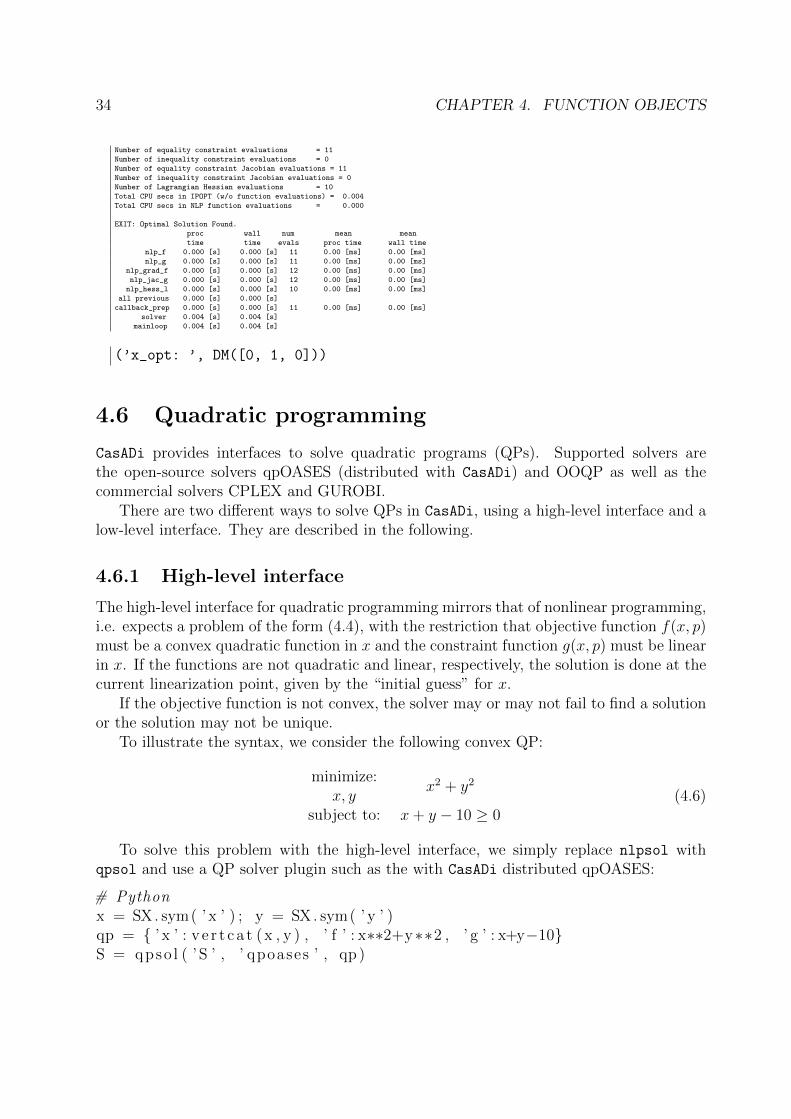
(’x_opt: ’, DM([0, 1, 0]))

4.6 Quadratic programming

CasADi provides interfaces to solve quadratic programs (QPs). Supported solvers arethe open-source solvers qpOASES (distributed with CasADi) and OOQP as well as thecommercial solvers CPLEX and GUROBI.

There are two different ways to solve QPs in CasADi, using a high-level interface and alow-level interface. They are described in the following.

4.6.1 High-level interface

The high-level interface for quadratic programming mirrors that of nonlinear programming,i.e. expects a problem of the form (4.4), with the restriction that objective function f(x, p)must be a convex quadratic function in x and the constraint function g(x, p) must be linearin x. If the functions are not quadratic and linear, respectively, the solution is done at thecurrent linearization point, given by the “initial guess” for x.

If the objective function is not convex, the solver may or may not fail to find a solutionor the solution may not be unique.

To illustrate the syntax, we consider the following convex QP:

minimize:x, y

x2 + y2

subject to: x+ y − 10 ≥ 0(4.6)

To solve this problem with the high-level interface, we simply replace nlpsol withqpsol and use a QP solver plugin such as the with CasADi distributed qpOASES:

# Pythonx = SX. sym( ’ x ’ ) ; y = SX. sym( ’ y ’ )qp = { ’ x ’ : v e r t c a t (x , y ) , ’ f ’ : x∗∗2+y∗∗2 , ’ g ’ : x+y−10}S = qpso l ( ’S ’ , ’ qpoases ’ , qp )

4.6. QUADRATIC PROGRAMMING 35

% MATLABx = SX. sym( ’ x ’ ) ; y = SX. sym( ’ y ’ )qp = s t r u c t ( ’ x ’ , [ x ; y ] , ’ f ’ : xˆ2+y ˆ2 , ’ g ’ , x+y−10)S = qpso l ( ’S ’ , ’ qpoases ’ , qp )

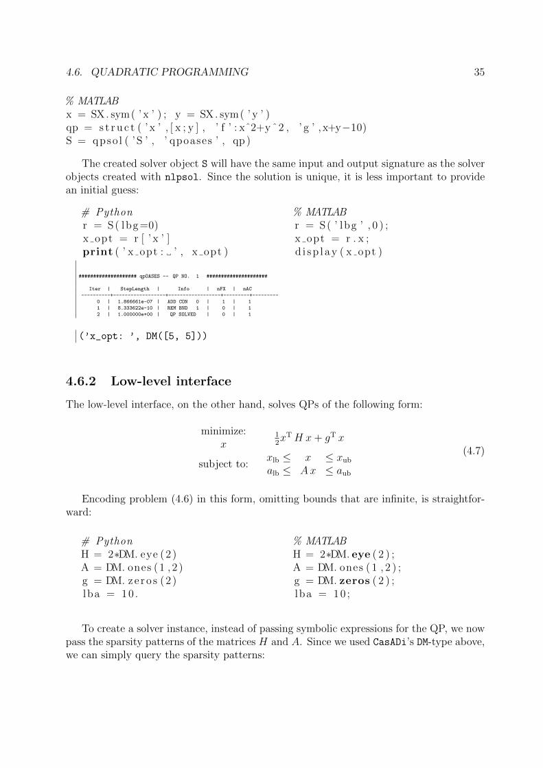
The created solver object S will have the same input and output signature as the solverobjects created with nlpsol. Since the solution is unique, it is less important to providean initial guess:

# Pythonr = S( lbg =0)x opt = r [ ’ x ’ ]print ( ’ x opt : ’ , x opt )

% MATLABr = S( ’ lbg ’ , 0 ) ;x opt = r . x ;d i sp l ay ( x opt )

#################### qpOASES -- QP NO. 1 #####################

Iter | StepLength | Info | nFX | nAC

----------+------------------+------------------+---------+---------

0 | 1.866661e-07 | ADD CON 0 | 1 | 1

1 | 8.333622e-10 | REM BND 1 | 0 | 1

2 | 1.000000e+00 | QP SOLVED | 0 | 1

(’x_opt: ’, DM([5, 5]))

4.6.2 Low-level interface

The low-level interface, on the other hand, solves QPs of the following form:

minimize:x

12xTH x+ gT x

subject to:xlb ≤ x ≤ xub

alb ≤ Ax ≤ aub

(4.7)

Encoding problem (4.6) in this form, omitting bounds that are infinite, is straightfor-ward:

# PythonH = 2∗DM. eye (2 )A = DM. ones (1 , 2 )g = DM. ze ro s (2 )lba = 10 .

% MATLABH = 2∗DM. eye ( 2 ) ;A = DM. ones ( 1 , 2 ) ;g = DM. zeros ( 2 ) ;lba = 10 ;

To create a solver instance, instead of passing symbolic expressions for the QP, we nowpass the sparsity patterns of the matrices H and A. Since we used CasADi’s DM-type above,we can simply query the sparsity patterns:


# Pythonqp = {}qp [ ’h ’ ] = H. s p a r s i t y ( )qp [ ’ a ’ ] = A. s p a r s i t y ( )S = con i c ( ’S ’ , ’ qpoases ’ , qp )

% MATLABqp = s t r u c t ;qp . h = H. s p a r s i t y ( ) ;qp . a = A. s p a r s i t y ( ) ;S = con i c ( ’S ’ , ’ qpoases ’ , qp ) ;

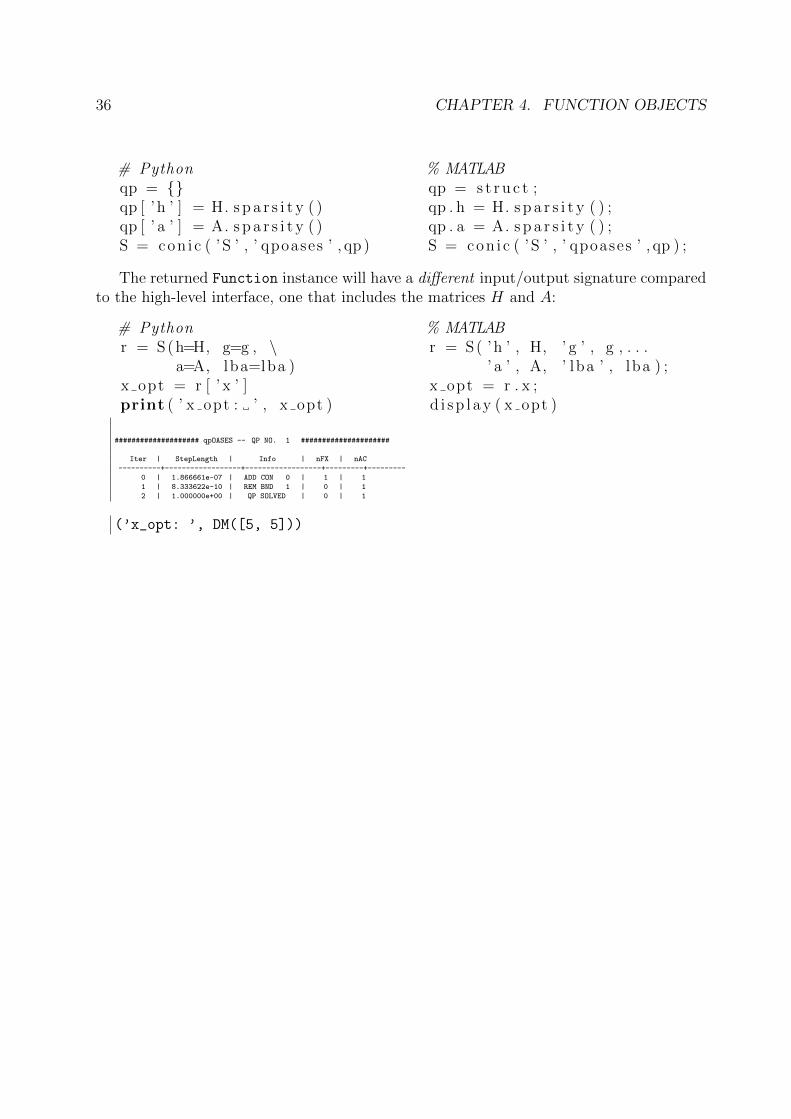
The returned Function instance will have a different input/output signature comparedto the high-level interface, one that includes the matrices H and A:

# Pythonr = S(h=H, g=g , \

a=A, lba=lba )x opt = r [ ’ x ’ ]print ( ’ x opt : ’ , x opt )

% MATLABr = S( ’h ’ , H, ’ g ’ , g , . . .

’ a ’ , A, ’ lba ’ , lba ) ;x opt = r . x ;d i sp l ay ( x opt )

#################### qpOASES -- QP NO. 1 #####################

Iter | StepLength | Info | nFX | nAC

----------+------------------+------------------+---------+---------

0 | 1.866661e-07 | ADD CON 0 | 1 | 1

1 | 8.333622e-10 | REM BND 1 | 0 | 1

2 | 1.000000e+00 | QP SOLVED | 0 | 1

(’x_opt: ’, DM([5, 5]))

Chapter 5

Generating C-code

The numerical evaluation of function objects in CasADi normally takes place in virtualmachines, implemented as part of CasADi’s symbolic framework. But CasADi also supportsthe generation of self-contained C-code for a large subset of function objects.

C-code generation is interesting for a number of reasons:

• Speeding up the evaluation time. As a rule of thumb, the numerical evaluation ofautogenerated code, compiled with code optimization flags, can be between 4 and 10times faster than the same code executed in CasADi’s virtual machines.

• Allowing code to be compiled on a system where CasADi is not installed, such as anembedded system. All that is needed to compile the generated code is a C compiler.

• Debugging and profiling functions. The generated code is essentially a mirror of theevaluation that takes place in the virtual machines and if a particular operation isslow, this is likely to show up when analysing the generated code with a profiling toolsuch as gprof. By looking at the code, it is also possible to detect what is potentiallydone in a suboptimal way. If the code is very long and takes a long time to compile,it is an indication that some functions need to be broken up in smaller, but nestedfunctions.

5.1 Syntax for generating code

Generated C code can be as simple as calling the generate member function for a Function

instance.

37

38 CHAPTER 5. GENERATING C-CODE


[ x , s i n ( y )∗x ] ,\[ ’ x ’ , ’ y ’ ] , [ ’ r ’ , ’ q ’ ] )

f . generate ( ’ gen . c ’ )


{x , sin ( y )∗x } , . . .{ ’ x ’ , ’ y ’ } ,{ ’ r ’ , ’ q ’ } ) ;

f . generate ( ’ gen . c ’ ) ;

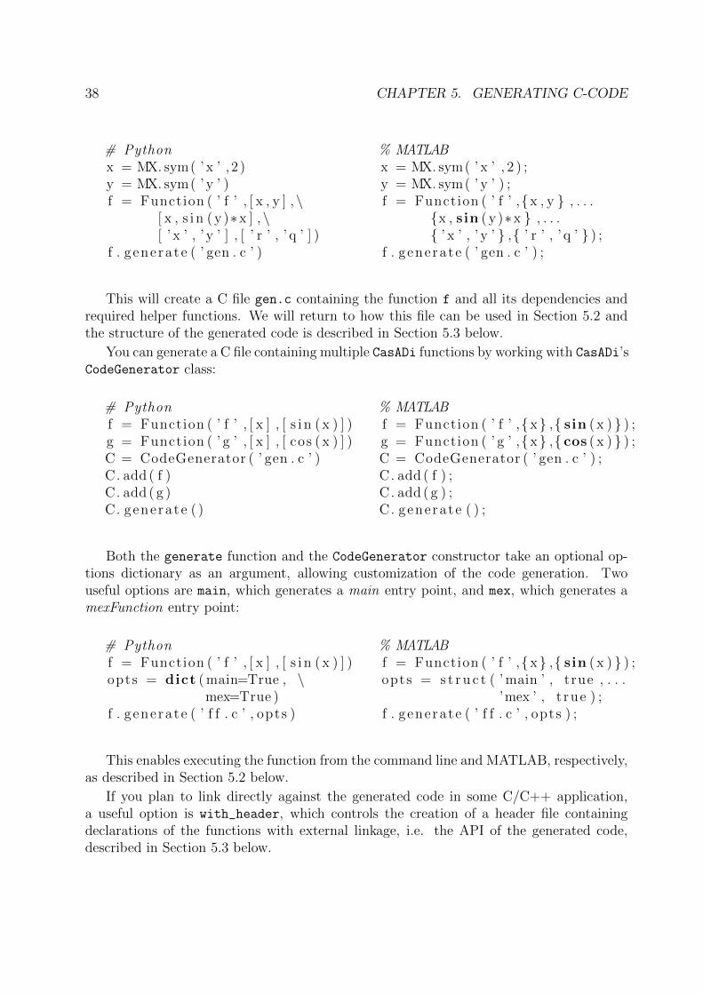
This will create a C file gen.c containing the function f and all its dependencies andrequired helper functions. We will return to how this file can be used in Section 5.2 andthe structure of the generated code is described in Section 5.3 below.

You can generate a C file containing multiple CasADi functions by working with CasADi’sCodeGenerator class:

# Pythonf = Function ( ’ f ’ , [ x ] , [ s i n ( x ) ] )g = Function ( ’ g ’ , [ x ] , [ cos ( x ) ] )C = CodeGenerator ( ’ gen . c ’ )C. add ( f )C. add ( g )C. generate ( )

% MATLABf = Function ( ’ f ’ ,{x} ,{ sin ( x ) } ) ;g = Function ( ’ g ’ ,{x} ,{ cos ( x ) } ) ;C = CodeGenerator ( ’ gen . c ’ ) ;C. add ( f ) ;C. add ( g ) ;C. generate ( ) ;

Both the generate function and the CodeGenerator constructor take an optional op-tions dictionary as an argument, allowing customization of the code generation. Twouseful options are main, which generates a main entry point, and mex, which generates amexFunction entry point:

# Pythonf = Function ( ’ f ’ , [ x ] , [ s i n ( x ) ] )opts = dict ( main=True , \

mex=True )f . generate ( ’ f f . c ’ , opts )

% MATLABf = Function ( ’ f ’ ,{x} ,{ sin ( x ) } ) ;opts = s t r u c t ( ’ main ’ , true , . . .

’mex ’ , t rue ) ;f . generate ( ’ f f . c ’ , opts ) ;

This enables executing the function from the command line and MATLAB, respectively,as described in Section 5.2 below.

If you plan to link directly against the generated code in some C/C++ application,a useful option is with_header, which controls the creation of a header file containingdeclarations of the functions with external linkage, i.e. the API of the generated code,described in Section 5.3 below.

5.2. USING THE GENERATED CODE 39

5.2 Using the generated code

The generated C code can be used in a number of different ways:

• The code can be compiled into a dynamically linked library (DLL), from which aFunction instance can be created using CasADi’s external function. Optionally,the user can rely on CasADi to carry out the compilation just-in-time.

• The generated code can be compiled into MEX function and executed from MAT-LAB.

• The generated code can be executed from the command line.

• The user can link, statically or dynamically, the generated code to his or her C/C++application, accessing the C API of the generated code.

• The code can be compiled into a dynamically linked library and the user can thenmanually access the C API using dlopen on Linux/OS X or LoadLibrary on Win-dows.

This is elaborated in the following.

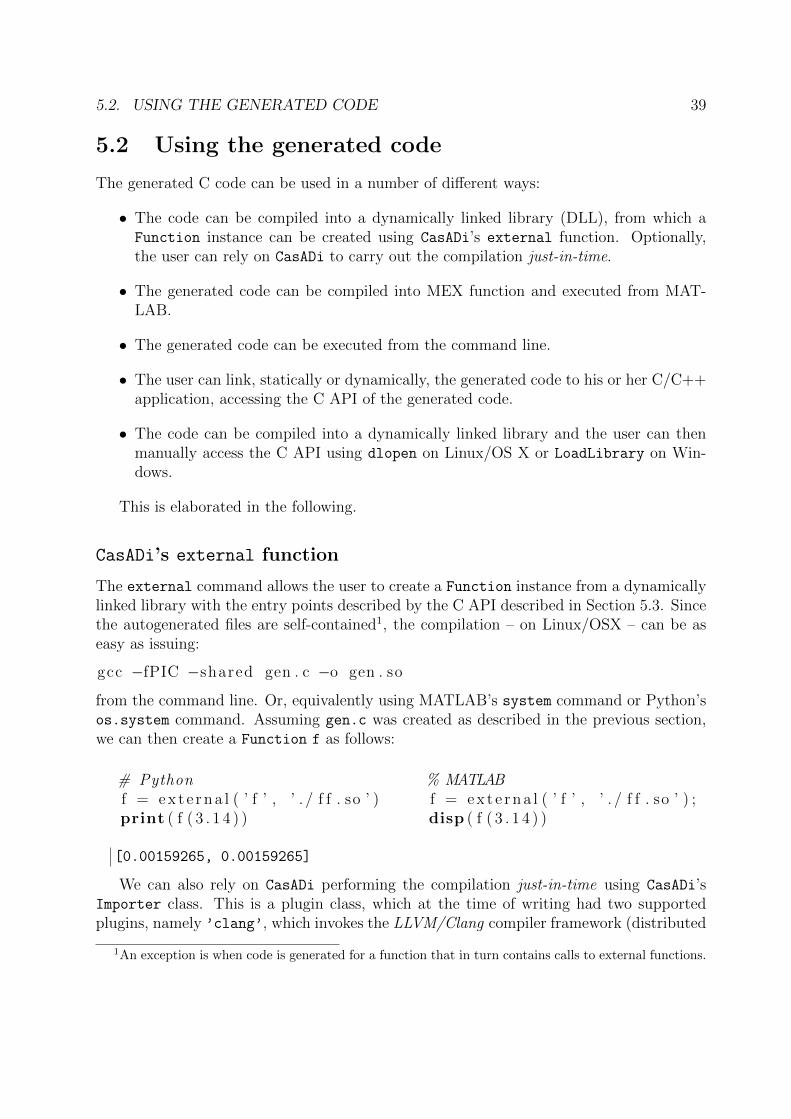
CasADi’s external function

The external command allows the user to create a Function instance from a dynamicallylinked library with the entry points described by the C API described in Section 5.3. Sincethe autogenerated files are self-contained1, the compilation – on Linux/OSX – can be aseasy as issuing:

gcc −fPIC −shared gen . c −o gen . so

from the command line. Or, equivalently using MATLAB’s system command or Python’sos.system command. Assuming gen.c was created as described in the previous section,we can then create a Function f as follows:

# Pythonf = e x t e r n a l ( ’ f ’ , ’ . / f f . so ’ )print ( f ( 3 . 1 4 ) )

% MATLABf = e x t e r n a l ( ’ f ’ , ’ . / f f . so ’ ) ;disp ( f ( 3 . 1 4 ) )

[0.00159265, 0.00159265]

We can also rely on CasADi performing the compilation just-in-time using CasADi’sImporter class. This is a plugin class, which at the time of writing had two supportedplugins, namely ’clang’, which invokes the LLVM/Clang compiler framework (distributed

1An exception is when code is generated for a function that in turn contains calls to external functions.


with CasADi), and ’shell’, which invokes the system compiler via the command line. Thelatter is only available on Linux/OS X:

# PythonC = Importer ( ’ f f . c ’ , ’ c lang ’ )f = e x t e r n a l ( ’ f ’ ,C) ;print ( f ( 3 . 1 4 ) )

% MATLABC = Importer ( ’ f f . c ’ , ’ c lang ’ ) ;f = e x t e r n a l ( ’ f ’ ,C) ;disp ( f ( 3 . 1 4 ) )

[0.00159265, 0.00159265]

We will return to the external function in Section 6.3.

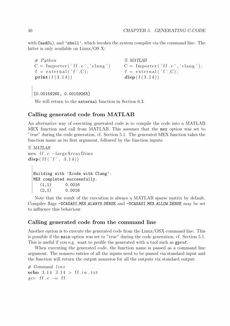
Calling generated code from MATLAB

An alternative way of executing generated code is to compile the code into a MATLABMEX function and call from MATLAB. This assumes that the mex option was set to”true” during the code generation, cf. Section 5.1. The generated MEX function takes thefunction name as its first argument, followed by the function inputs:

% MATLABmex f f . c −largeArrayDimsdisp ( f f ( ’ f ’ , 3 . 1 4 ) )

Building with ’Xcode with Clang’.

MEX completed successfully.

(1,1) 0.0016

(2,1) 0.0016

Note that the result of the execution is always a MATLAB sparse matrix by default.Compiler flags -DCASASI MEX ALWAYS DENSE and -DCASASI MEX ALLOW DENSE may be setto influence this behaviour.

Calling generated code from the command line

Another option is to execute the generated code from the Linux/OSX command line. Thisis possible if the main option was set to ”true” during the code generation, cf. Section 5.1.This is useful if you e.g. want to profile the generated with a tool such as gprof.

When executing the generated code, the function name is passed as a command lineargument. The nonzero entries of all the inputs need to be passed via standard input andthe function will return the output nonzeros for all the outputs via standard output:

# Command l i n eecho 3 .14 3 .14 > f f i n . txtgcc f f . c −o f f

5.3. API OF THE GENERATED CODE 41

. / f f f < f f i n . txt > f f o u t . txtcat f f o u t . txt

0.00159265 0.00159265

Linking against generated code from a C/C++ application

The generated code is written so that it can be linked with directly from a C/C++ applica-tion. If the with_header option was set to ”true” during the code generation, a header filewith declarations of all the exposed entry points of the file. Using this header file requiresan understanding of CasADi’s codegen API, as described in Section 5.3 below. Symbolsthat are not exposed are prefixed with a file-specific prefix, allowing an application to linkagainst multiple generated functions without risking symbol conflicts.

Dynamically loading generated code from a C/C++ application

A variant of above is to compile the generated code into a shared library, but directlyaccessing the exposed symbols rather than relying on CasADi’s external function. Thisalso requires an understanding of the structure of the generated code.

In CasADi’s example collection, codegen_usage.cpp demonstrates how this can bedone.

5.3 API of the generated code

The API of the generated code consists of a number of functions with external linkage.In addition to the actual execution, there are functions for memory management as wellas meta information about the inputs and outputs. These functions are described in thefollowing. Below, assume that the name of function we want to access is fname. To seewhat these functions actually look like in code and when they are called, we refer to thecodegen_usage.cpp example.

Reference counting

void f name inc r e f ( void ) ;void fname decre f ( void ) ;

A generated function may need to e.g. read in some data or initialize some datastructures before first call. This is typically not needed for functions generated from CasADi

expressions, but may be required e.g. when the generated code contains calls to externalfunctions. Similarly, memory might need to be deallocated after usage.

To keep track of the ownership, the generated code contains two functions for increasingand decreasing a reference counter. They are named fname_incref and fname_decref,respectively. These functions have no input argument and return void.


Typically, some initialization may take place upon the first call to fname_incref andsubsequent calls will only increase some internal counter. The fname_decref, on the otherhand, decreases the internal counter and when the counter hits zero, a deallocation – ifany – takes place.

Number of inputs and outputs

int fname n in ( void ) ;int fname n out ( void ) ;

The number of function inputs and outputs can be obtained by calling the fname_n_in

and fname_n_out functions, respectively. These functions take no inputs and return thenumber of input or outputs.

Names of inputs and outputs

const char∗ fname name in ( int ind ) ;const char∗ fname name out ( int ind ) ;

The functions fname_name_in and fname_name_out return the name of a particularinput or output. They take the index of the input or output, starting with index 0, andreturn a const char* with the name as a null-terminated C string. Upon failure, thesefunctions will return a null pointer.

Sparsity patterns of inputs and outputs

const int∗ f n a m e s p a r s i t y i n ( int ind ) ;const int∗ f name spa r s i t y ou t ( int ind ) ;

The sparsity pattern for a given input or output is obtained by calling fname_sparsity_inand fname_sparsity_out, respectively. These functions take the input or output indexand return a pointer to a field of constant integers (const int*). This is a compact repre-sentation of the compressed column storage (CCS) format that CasADi uses, cf. Section 3.5.The integer field pointed to is structured as follows:• The first two entries are the number of rows and columns, respectively. In the

following referred to as nrow and ncol.

• If the third entry is 1, the pattern is dense and any remaining entries are discarded.

• If the third entry is 0, that entry plus subsequent ncol entries form the nonzero offsetsfor each column, colind in the following. E.g. column i will consist of the nonzeroindices ranging from colind[i] to colind[i + 1]. The last entry, colind[ncol], willbe equal to the number of nonzeros, nnz.

• Finally, if the sparsity pattern is not dense, i.e. if nnz 6= nrow ∗ ncol, then the lastnnz entries will contain the row indices.

Upon failure, these functions will return a null pointer.

5.3. API OF THE GENERATED CODE 43

Maximum number of memory objects

int fname n mem ( void ) ;

A function may contain some mutable memory, e.g. for caching the latest factorizationor keeping track of evaluation statistics. When multiple functions need to call the samefunction without conflicting, they each need to work with a different memory object. Thisis especially important for evaluation in parallel on a shared memory architecture, in whichcase each thread should access a different memory object.

The function fname_n_mem returns the maximum number of memory objects or 0 ifthere is no upper bound.

Work vectors

int fname work ( int∗ s z arg , int∗ s z r e s , int∗ sz iw , int∗ sz w ) ;

To allow the evaluation to be performed efficiently with a small memory footprint, theuser is expected to pass four work arrays. The function fname_work returns the lengthof these arrays, which have entries of type const double*, double*, int and double,respectively.

The return value of the function is nonzero upon failure.

Numerical evaluation

int fname ( const double∗∗ arg , double∗∗ res ,int∗ iw , double∗ w, int mem) ;

Finally, the function fname, performs the actual evaluation. It takes as input argumentsthe four work vectors and the index of the chosen memory object. The length of the workvectors must be at least the lengths provided by the fname work command and the indexof the memory object must be strictly smaller than the value returned by fname n mem.

The nonzeros of the function inputs are pointed to by the first entries of the arg workvector and are unchanged by the evaluation. Similarly, the output nonzeros are pointedto by the first entries of the res work vector and are also unchanged (i.e. the pointers areunchanged, not the actual values).

The return value of the function is nonzero upon failure.


Chapter 6

User-defined function objects

There are situations when rewriting user-functions using CasADi symbolics is not possibleor practical. To tackle this, CasADi provides a number of ways to embed a call to a ”blackbox” function defined in the language CasADi is being used from (C++, MATLAB orPython) or in C. That being said, the recommendation is always to try to avoid this whenpossible, even if it means investing a lot of time reimplementing existing code. Functionsdefined using CasADi symbolics are almost always more efficient, especially when derivativecalculation is involved, since a lot more structure can typically be exploited.

Depending on the circumstances, the user can implement custom Function objects ina number of different ways:

• Subclassing FunctionInternal

• Subclassing Callback

• Importing a function with external

We elaborate on this in the following.

6.1 Subclassing FunctionInternal

All function objects presented in Chapter 4 are implemented in CasADi as C++ classesinheriting from the FunctionInternal abstract base class. In principle, a user with fa-miliarity with C++ programming, should be able to implement a class inheriting fromFunctionInternal, implementing the virtual methods of this class. The best referencefor doing so is the C++ API documentation, choosing ”switch to internal” to expose theinternal API.

Since FunctionInternal is not considered part of the stable, public API, we adviceagainst this in general, unless the plan is to make a contribution to CasADi.

45

46 CHAPTER 6. USER-DEFINED FUNCTION OBJECTS

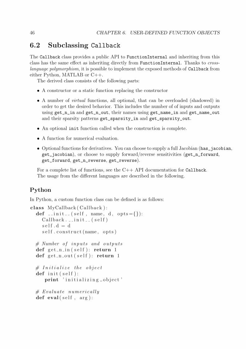
6.2 Subclassing Callback

The Callback class provides a public API to FunctionInternal and inheriting from thisclass has the same effect as inheriting directly from FunctionInternal. Thanks to cross-language polymorphism, it is possible to implement the exposed methods of Callback fromeither Python, MATLAB or C++.

The derived class consists of the following parts:

• A constructor or a static function replacing the constructor

• A number of virtual functions, all optional, that can be overloaded (shadowed) inorder to get the desired behavior. This includes the number of of inputs and outputsusing get_n_in and get_n_out, their names using get_name_in and get_name_out

and their sparsity patterns get_sparsity_in and get_sparsity_out.

• An optional init function called when the construction is complete.

• A function for numerical evaluation.

• Optional functions for derivatives. You can choose to supply a full Jacobian (has_jacobian,get_jacobian), or choose to supply forward/reverse sensitivities (get_n_forward,get_forward, get_n_reverse, get_reverse).

For a complete list of functions, see the C++ API documentation for Callback.The usage from the different languages are described in the following.

Python

In Python, a custom function class can be defined is as follows:

class MyCallback ( Cal lback ) :def i n i t ( s e l f , name , d , opts ={}):

Cal lback . i n i t ( s e l f )s e l f . d = ds e l f . c on s t ruc t (name , opts )

# Number o f i n p u t s and o u t p u t sdef g e t n i n ( s e l f ) : return 1def ge t n out ( s e l f ) : return 1

# I n i t i a l i z e the o b j e c tdef i n i t ( s e l f ) :

print ’ i n i t i a l i z i n g ob j e c t ’

# Evaluate numer ica l l ydef eval ( s e l f , arg ) :

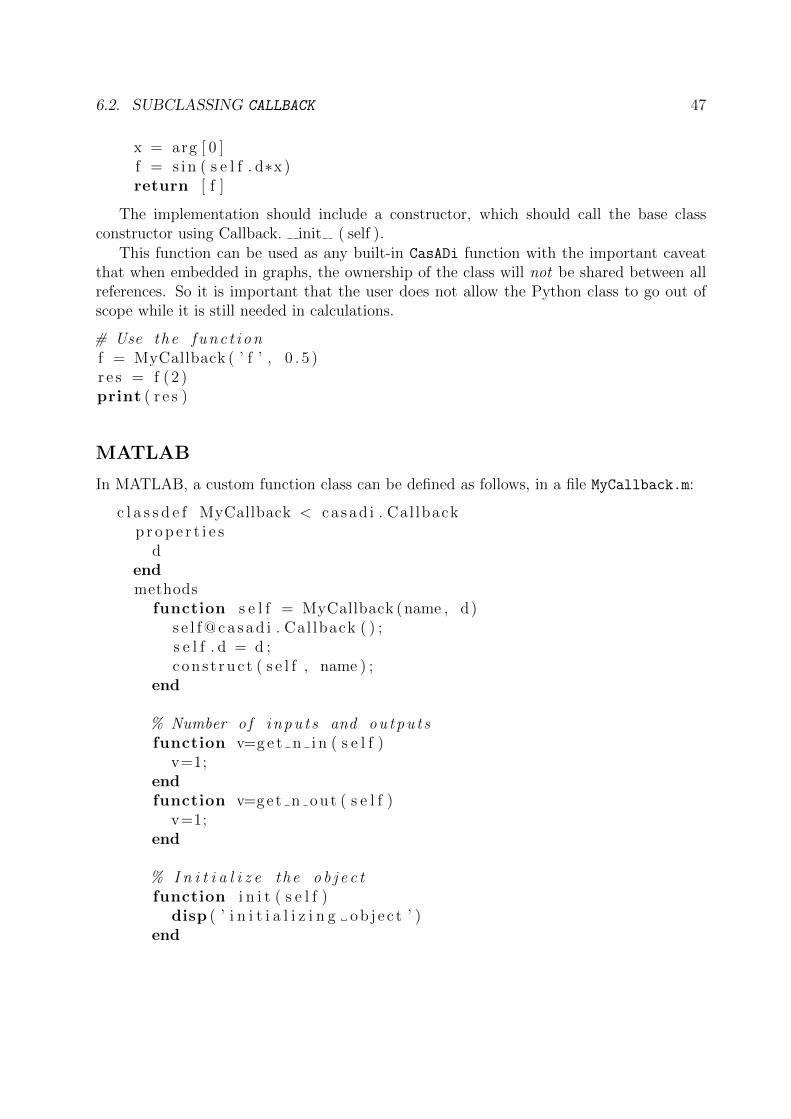
6.2. SUBCLASSING CALLBACK 47

x = arg [ 0 ]f = s i n ( s e l f . d∗x )return [ f ]

The implementation should include a constructor, which should call the base classconstructor using Callback. init ( self ).

This function can be used as any built-in CasADi function with the important caveatthat when embedded in graphs, the ownership of the class will not be shared between allreferences. So it is important that the user does not allow the Python class to go out ofscope while it is still needed in calculations.

# Use the f u n c t i o nf = MyCallback ( ’ f ’ , 0 . 5 )r e s = f (2 )print ( r e s )

MATLAB

In MATLAB, a custom function class can be defined as follows, in a file MyCallback.m:

c l a s s d e f MyCallback < ca sad i . Cal lbackp r o p e r t i e s

dendmethods

function s e l f = MyCallback (name , d)s e l f @ c a s a d i . Cal lback ( ) ;s e l f . d = d ;cons t ruc t ( s e l f , name ) ;

end

% Number o f i n p u t s and o u t p u t sfunction v=g e t n i n ( s e l f )

v=1;endfunction v=get n out ( s e l f )

v=1;end

% I n i t i a l i z e the o b j e c tfunction i n i t ( s e l f )

disp ( ’ i n i t i a l i z i n g ob j e c t ’ )end


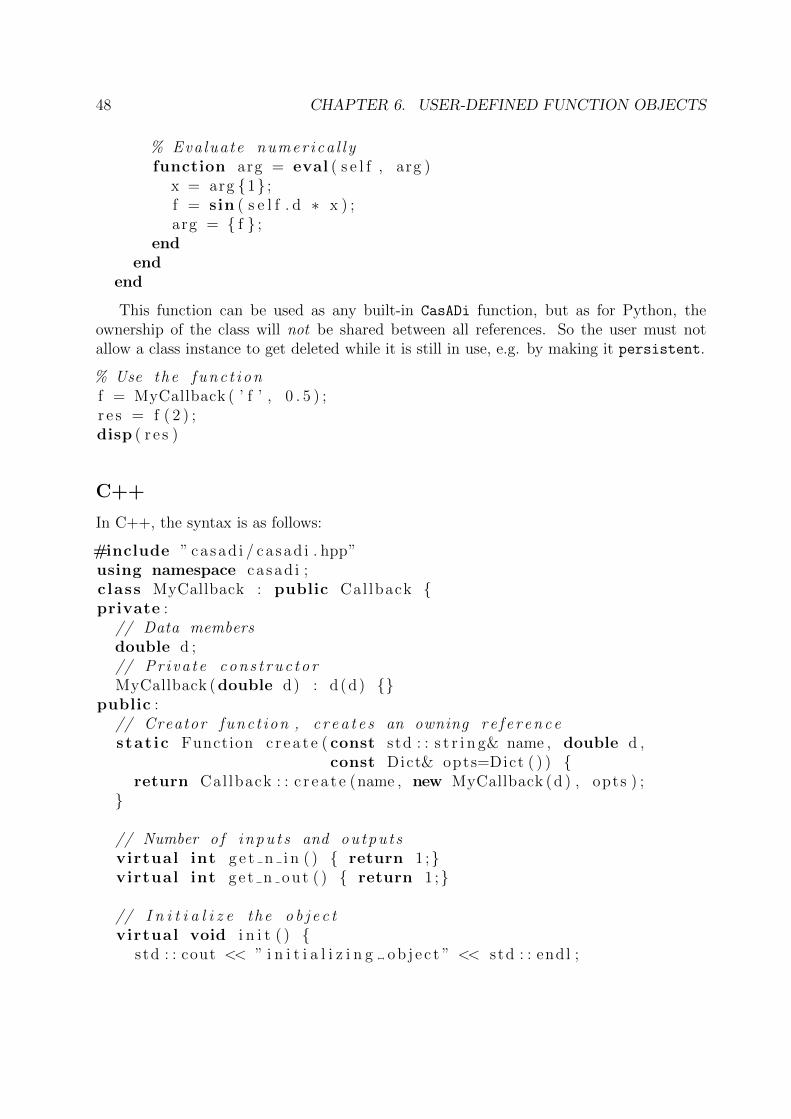
% Evaluate numer ica l l yfunction arg = eval ( s e l f , arg )

x = arg {1} ;f = sin ( s e l f . d ∗ x ) ;arg = { f } ;

endend

end

This function can be used as any built-in CasADi function, but as for Python, theownership of the class will not be shared between all references. So the user must notallow a class instance to get deleted while it is still in use, e.g. by making it persistent.

% Use the f u n c t i o nf = MyCallback ( ’ f ’ , 0 . 5 ) ;r e s = f ( 2 ) ;disp ( r e s )

C++

In C++, the syntax is as follows:

#include ” ca sad i / ca sad i . hpp”using namespace ca sad i ;class MyCallback : public Cal lback {private :

// Data membersdouble d ;// P r i v a t e c o n s t r u c t o rMyCallback (double d) : d(d) {}

public :// Creator func t ion , c r e a t e s an owning r e f e r e n c estat ic Function c r e a t e ( const std : : s t r i n g& name , double d ,

const Dict& opts=Dict ( ) ) {return Cal lback : : c r e a t e (name , new MyCallback (d ) , opts ) ;

}

// Number o f i n p u t s and o u t p u t svirtual int g e t n i n ( ) { return 1 ;}virtual int ge t n out ( ) { return 1 ;}

// I n i t i a l i z e the o b j e c tvirtual void i n i t ( ) {

std : : cout << ” i n i t i a l i z i n g ob j e c t ” << std : : endl ;

6.3. IMPORTING A FUNCTION WITH EXTERNAL 49

}

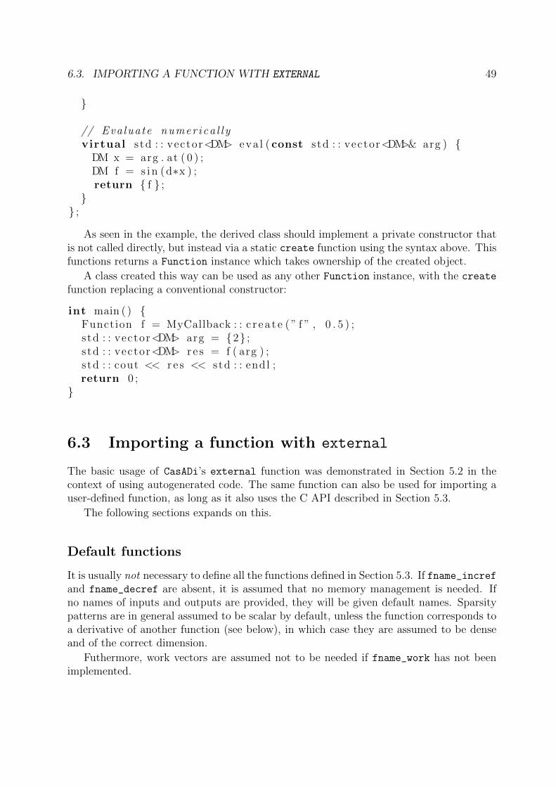
// Eva luate numer ica l l yvirtual std : : vector<DM> eva l ( const std : : vector<DM>& arg ) {

DM x = arg . at ( 0 ) ;DM f = s i n (d∗x ) ;return { f } ;

}} ;

As seen in the example, the derived class should implement a private constructor thatis not called directly, but instead via a static create function using the syntax above. Thisfunctions returns a Function instance which takes ownership of the created object.

A class created this way can be used as any other Function instance, with the create

function replacing a conventional constructor:

int main ( ) {Function f = MyCallback : : c r e a t e ( ” f ” , 0 . 5 ) ;s td : : vector<DM> arg = {2} ;s td : : vector<DM> r e s = f ( arg ) ;s td : : cout << r e s << std : : endl ;return 0 ;

}

6.3 Importing a function with external

The basic usage of CasADi’s external function was demonstrated in Section 5.2 in thecontext of using autogenerated code. The same function can also be used for importing auser-defined function, as long as it also uses the C API described in Section 5.3.

The following sections expands on this.

Default functions

It is usually not necessary to define all the functions defined in Section 5.3. If fname_increfand fname_decref are absent, it is assumed that no memory management is needed. Ifno names of inputs and outputs are provided, they will be given default names. Sparsitypatterns are in general assumed to be scalar by default, unless the function corresponds toa derivative of another function (see below), in which case they are assumed to be denseand of the correct dimension.

Futhermore, work vectors are assumed not to be needed if fname_work has not beenimplemented.


Meta information as comments

If you rely on CasADi’s just-in-time compiler, you can provide meta information as acomment in the C code instead of implementing the actual callback function.

The structure of such meta information should be as follows:

/∗CASADIMETA: fname N IN 1: fname N OUT 2: fname NAME IN [ 0 ] x: fname NAME OUT [ 0 ] r: fname NAME OUT [ 1 ] s: fname SPARSITY IN [ 0 ] 2 1 0 2∗/

Simplified evaluation signature

If all the inputs and outputs are scalars, the user can choose to replace the function fornumerical evaluation:

int fname ( const double∗∗ arg , double∗∗ res ,int∗ iw , double∗ w, int mem) ;

with a function with simpler syntax:

void fname simple ( const double∗ arg , double∗ r e s ) ;

Note that _simple must be appended to the function name. Evaluating a functionwith this syntax potentially carries less overhead.

Derivatives

The external function can be made differentiable by providing functions for calculatingderivatives. During derivative calculations, CasADi will look for symbols in the samefile/shared library that follows a certain naming convention. For example, you can specifya Jacobian for all the outputs with respect to all inputs for a function named fname

by implementing a function named jac_fname. Similary, you can specify a function forcalculating one forward directional derivative by providing a function named fwd1_fname,where 1 can be replaced by 2, 4, 8, 16, 32 or 64 for calculating multiple forward directionalderivatives at once. For reverse mode directional derivatives, replace fwd with adj.

This is an experimental feature.

Chapter 7

The DaeBuilder class

The DaeBuilder class in CasADi is an auxiliary class intended to facilitate the modelingcomplex dynamical systems for later use with optimal control algorithms. This class canbe seen as a low-level alternative to a physical modeling language such as Modelica (cf.Section 7.3), while still being higher level than working directly with CasADi symbolicexpressions. Another important usage it to provide an interface to physical modelinglanguages and software and be a building blocks for developing domain specific modelingenvironments.

Using the DaeBuilder class consists of the following steps:

• Step-by-step constructing a structured system of differential-algebraic equations (DAE)or, alternatively, importing an existing model from Modelica

• Symbolically reformulate the DAE

• Generate a chosen set of CasADi functions to be used for e.g. optimal control or Ccode generation

In the following sections, we describe the mathematical formulation of the class and itsintended usage.

7.1 Mathematical formulation

The DaeBuilder class uses a relatively rich problem formulation that consists of a set ofinput expressions and a set of output expressions, each defined by a string identifier. Thechoice of expressions was inspired by the functional mockup interface (FMI) version 2.0 1

Input expressions

’t’ Time t

1FMI development group. Functional Mock-up Interface for Model Exchange and Co-Simulation.https://www.fmi-standard.org/, July 2014. Specification, FMI 2.0. Section 3.1, pp. 7172

51

https://www.fmi-standard.org/

52 CHAPTER 7. THE DAEBUILDER CLASS

’c’ Named constants c

’p’ Independent parameters p

’d’ Dependent parameters d, depends only on p and c and, acyclically, on other d

’x’ Differential state x, defined by an explicit ODE

’s’ Differential state s, defined by an implicit ODE

’sdot’ Time derivatives implicitly defined differential state s

’z’ Algebraic variable, defined by an algebraic equation

’q’ Quadrature state q. A differential state that may not appear in the right-hand-sideand hence can be calculated by quadrature formulas.

’w’ Local variables w. Calculated from time and time dependent variables. They mayalso depend, acyclically, on other w.

’y’ Output variables y

Output expressions

The above input expressions are used to define the following output expressions:

’ddef’ Explicit expression for calculating d

’wdef’ Explicit expression for calculating w

’ode’ The explicit ODE right-hand-side: x = ode(t, w, x, s, z, u, p, d)

’dae’ The implicit ODE right-hand-side: dae(t, w, x, s, z, u, p, d, s) = 0

’alg’ The algebraic equations: alg(t, w, x, s, z, u, p, d) = 0

’quad’ The quadrature equations: q = quad(t, w, x, s, z, u, p, d)

’ydef’ Explicit expressions for calculating y

7.2 Constructing a DaeBuilder instance

Consider the following simple DAE corresponding to a controlled rocket subject to quadraticair friction term and gravity, which loses mass as it uses up fuel:

h = v, h(0) = 0 (7.1a)

v = (u− a v2)/m− g, v(0) = 0 (7.1b)

m = −b u2, m(0) = 1 (7.1c)

7.3. IMPORT OF OCPS FROM MODELICA 53

where the three states correspond to height, velocity and mass, respectively. u is the thrustof the rocket and (a, b) are parameters.

To construct a DAE formulation for this problem, start with an empty DaeBuilder

instance and add the input and output expressions step-by-step as follows.

# Pythondae = DaeBuilder ( )# Add input e x p r e s s i o n sa = dae . add p ( ’ a ’ )b = dae . add p ( ’b ’ )u = dae . add u ( ’u ’ )h = dae . add x ( ’h ’ )v = dae . add x ( ’ v ’ )m = dae . add x ( ’m’ )# Add output e x p r e s s i o n shdot = vvdot = (u−a∗v∗∗2)/m−gmdot = −b∗u∗∗2dae . add ode ( hdot )dae . add ode ( vdot )dae . add ode (mdot )# S p e c i f y i n i t i a l c o n d i t i o n sdae . s e t s t a r t ( ’h ’ , 0)dae . s e t s t a r t ( ’ v ’ , 0)dae . s e t s t a r t ( ’m’ , 1)# Add meta in format iondae . s e t u n i t ( ’h ’ , ’m’ )dae . s e t u n i t ( ’ v ’ , ’m/ s ’ )dae . s e t u n i t ( ’m’ , ’ kg ’ )

% MATLABdae = DaeBuilder ;% Add input e x p r e s s i o n sa = dae . add p ( ’ a ’ ) ;b = dae . add p ( ’b ’ ) ;u = dae . add u ( ’u ’ ) ;h = dae . add x ( ’h ’ ) ;v = dae . add x ( ’ v ’ ) ;m = dae . add x ( ’m’ ) ;% Add output e x p r e s s i o n shdot = v ;vdot = (u−a∗vˆ2)/m−g ;mdot = −b∗u ˆ2 ;dae . add ode ( hdot ) ;dae . add ode ( vdot ) ;dae . add ode (mdot ) ;% S p e c i f y i n i t i a l c o n d i t i o n sdae . s e t s t a r t ( ’h ’ , 0 ) ;dae . s e t s t a r t ( ’ v ’ , 0 ) ;dae . s e t s t a r t ( ’m’ , 1 ) ;% Add meta in format iondae . s e t u n i t ( ’h ’ , ’m’ ) ;dae . s e t u n i t ( ’ v ’ , ’m/ s ’ ) ;dae . s e t u n i t ( ’m’ , ’ kg ’ ) ;

Other input and output expressions can be added in an analogous way. For a full listof functions, see the C++ API documentation for DaeBuilder.

7.3 Import of OCPs from Modelica

An alternative to model directly in CasADi, as above, is to use an advanced physicalmodeling language such as Modelica to specity the model. For this, CasADi offers interop-erability with the open-source JModelica.org compiler, which is written specifically withoptimal control in mind. Model inport from JModelica.org is possible in two different ways;using the JModelica.org’s CasadiInterface or via DaeBuilder’s parse fmi command.

We recommend the former approach, since it is being actively maintained and refer toJModelica.org’s user guide for details on how to extract CasADi expressions.

In the following, we will outline the legacy approach, using parse fmi.

http://www.jmodelica.org/


Legacy import of a modelDescription.xml file

To see how to use the Modelica import, look at thermodynamics example.py and cstr.cppin CasADi’s example collection.

Assuming that the Modelica/Optimica model ModelicaClass.ModelicaModel is de-fined in the files file1.mo and file2.mop, the Python compile command is:

from pymodelica import compile jmujmu name=compile jmu ( ’ Model icaClass . ModelicaModel ’ , \

[ ’ f i l e 1 .mo ’ , ’ f i l e 2 .mop ’ ] , ’ auto ’ , ’ ipopt ’ ,\{ ’ g ene ra t e xml equat i ons ’ : True , ’ generate fmi me xml ’ : Fa l se })

This will generate a jmu-file, which is essentially a zip file containing, among otherthings, the file modelDescription.xml. This XML-file contains a symbolic representationof the optimal control problem and can be inspected in a standard XML editor.

from z i p f i l e import Z ipF i l es f i l e = Z ipF i l e ( jmu name ’ , ’ r ’ )m f i l e = s f i l e . e x t r a c t ( ’ mode lDescr ipt ion . xml ’ , ’ . ’ )

Once a modelDescription.xml file is available, it can be imported using the parse fmicommand:

dae = DaeBuilder ( )ocp . pa r s e fm i ( ’ mode lDescr ipt ion . xml ’ )

7.4 Symbolic reformulation

One of the original purposes of the DaeBuilder class was to reformulate a fully-implicitDAE, typically coming from Modelica, to a semi-explicit DAE that can be used morereadily in optimal control algorithms.

This can be done by the make implicit command:

# Pythonocp . make exp l i c i t ( )

% MATLABocp . make exp l i c i t ( ) ;

Other useful commands available for an instance ocp of DaeBuilder include:

print ocp Print the optimal optimal control problem to screen

ocp.scale variables() Scale all variables using the nominal attribute for each variable

ocp.eliminate d() Eliminate all independent parameters from the symbolic expressions

For a more detailed description of this class and its functionalities, we again refer tothe API documentation.

https://github.com/casadi/casadi/blob/tested/examples/python/modelica/fritzson_application_examples/thermodynamics_example.py

https://github.com/casadi/casadi/blob/tested/examples/cplusplus/cstr.cpp

7.5. FUNCTION FACTORY 55

7.5 Function factory

Once a DaeBuilder has been formulated and possibily reformulated to a satisfactory form,we can generate CasADi functions corresponding to the input and output expressions out-lined in Section 7.1. For example, to create a function for the ODE right-hand-side for therocket model in Section 7.2, simply provide a display name of the function being created,a list of input expressions and a list of output expressions:

# Pythonf = dae . c r e a t e ( ’ f ’ ,\

[ ’ x ’ , ’ u ’ , ’ p ’ ] , [ ’ ode ’ ] )

% MATLABf = dae . c r e a t e ( ’ f ’ , . . .

{ ’ x ’ , ’ u ’ , ’ p ’ } ,{ ’ ode ’ } ) ;

Using a naming convention, we can also create Jacobians, e.g. for the ’ode’ output withrespect to ’x’:

# Pythonf = dae . c r e a t e ( ’ f ’ ,\

[ ’ x ’ , ’ u ’ , ’ p ’ ] ,\[ ’ j a c o d e x ’ ] )

% MATLABf = dae . c r e a t e ( ’ f ’ , . . .

{ ’ x ’ , ’ u ’ , ’ p ’ } ,{ ’ j a c o d e x ’ } ) ;

Functions with second order information can be extracted by first creating a namedlinear combination of the output expressions using add lc and then requesting its Hessian:

# Pythondae . add l c ( ’gamma ’ , [ ’ ode ’ ] )hes = dae . c r e a t e ( ’ h e s ,\

[ ’ x ’ , ’ u ’ , ’ p ’ , ’ lam ode ’ ] ,\[ ’ hes gamma x x ’ ] )

% MATLABdae . add l c ( ’gamma,{ ’ ode ’ } ) ;hes = dae . c r e a t e ( h e s , . . .{ ’ x ’ , ’ u ’ , ’ p ’ , ’ lam ode ’ } , . . .{ ’ hes gamma x x ’ } ) ;

It is also possible to simply extract the symbolic expressions from the DaeBuilder

instance and manually create CasADi functions. For example, dae.x contains all the ex-pressions corresponding to ’x’, dae.ode contains the expressions corresponding to ’ode’,etc.


Chapter 8

Optimal control with CasADi

CasADi can be used to solve optimal control problems (OCP) using a variety of meth-ods, including direct (a.k.a. discretize-then-optimize) and indirect (a.k.a. optimize-then-discretize) methods, all-at-once (e.g. collocation) methods and shooting-methods requiringembedded solvers of initial value problems in ODE or DAE. As a user, you are in generalexpected to write your own OCP solver and CasADi aims as making this as easy as possibleby providing powerful high-level building blocks. Since you are writing the solver yourself(rather than calling an existing “black-box” solver), a basic understanding of how to solveOCPs is indispensable. Good, self-contained introductions to numerical optimal controlcan be found in the recent textbooks by Biegler1 or Betts2 or Moritz Diehl’s lecture noteson numerical optimal control.

8.1 A simple test problem

To illustrate some of the methods, we will consider the following test problem, namelydriving a Van der Pol oscillator to the origin, while trying to minimize a quadratic cost:

minimize:x(·) ∈ R2, u(·) ∈ R

∫ T

t=0

(x20 + x2

1 + u2) dt

subject to:x0 = (1− x2

1)x0 − x1 + ux1 = x0

−1.0 ≤ u ≤ 1.0, x1 ≥ −0.25for 0 ≤ t ≤ T

x0(0) = 0, x1(0) = 1,

(8.1)

with T = 10.

1Lorenz T. Biegler, Nonlinear Programming: Concepts, Algorithms, and Applications to Chemical Pro-cesses, SIAM 2010

2John T. Betts, Practical Methods for Optimal Control Using Nonlinear Programming, SIAM 2001

57

http://homes.esat.kuleuven.be/~mdiehl/NUMOPT/numopt.pdf

http://books.google.es/books/about/Nonlinear_Programming.html?id=VdB1wJQu0sgC&redir_esc=y

http://books.google.es/books/about/Nonlinear_Programming.html?id=VdB1wJQu0sgC&redir_esc=y

http://books.google.es/books/about/Practical_Methods_for_Optimal_Control_Us.html?id=Yn53JcYAeaoC&redir_esc=y

58 CHAPTER 8. OPTIMAL CONTROL WITH CASADI

In CasADi’s examples collection3, you find codes for solving optimal control problemsusing a variety of different methods.

In the following, we will discuss three of the most important methods, namely directsingle shooting, direct collocation and direct collocation.

8.2 Direct single-shooting

In the direct single shooting method, the control trajectory is parametrized using somepiecewise smooth approximation, typically piecewise constant.

Using an explicit expression for the controls, we can then eliminate the whole statetrajectory from the optimization problem, ending up with an NLP in only the discretizedcontrols.

In CasADi’s examples collection, you will find the codes direct_single_shooting.pyand direct_single_shooting.m for Python and MATLAB/Octave, respectively. Thesecodes implement the direct single shooting method and solves it with IPOPT, relyingCasADi to calculate derivatives. To obtain the discrete time dynamics from the continuoustime dynamics, a simple fixed-step Runge-Kutta 4 (RK4) integrator is implemented usingCasADi symbolics. Simple integrator codes like these are often useful in the context ofoptimal control, but care must be taken so that they accuractely solves the initial-valueproblem.

The code also shows how the RK4 scheme can be replaced by a more advanced in-tegrator, namely the CVODES integrator from the SUNDIALS suite, which implementsa variable stepsize, variable order backward differentiation formula (BDF) scheme. Anadvanced integrator like this is useful for larger systems, systems with stiff dynamics, forDAEs and for checking a simpler scheme for consistency.

8.3 Direct multiple-shooting

The direct_multiple_shooting.py and direct_multiple_shooting.m codes, also inCasADi’s examples collection, implement the direct multiple shooting method. This is verysimilar to the direct single shooting method, but includes the state at certain shooting nodesas decision variables in the NLP and includes equality constraints to ensure continuity ofthe trajectory.

The direct multiple shooting method is often superior to the direct single shootingmethod, since ”lifting” the problem to a higher dimension is known to often improveconvergence. The user is also able to initialize with a known guess for the state trajectory.

The drawback is that the NLP solved gets much larger, although this is often compen-sated by the fact that it is also much sparser.

3You can obtain this collection as an archive named examples pack.zip in CasADi’s download area

http://files.casadi.org

8.4. DIRECT COLLOCATION 59

8.4 Direct collocation

Finally, the direct_collocation.py and direct_collocation.m codes implement thedirect collocation method. In this case, a parametrization of the entire state trajectory,as piecewise low-order polynomials, are included as decision variables in the NLP. Thisremoves the need for the formulation of the discrete time dynamics completely.

The NLP in direct collocation is even larger than that in direct multiple shooting, butis also even sparser.

60 CHAPTER 8. OPTIMAL CONTROL WITH CASADI

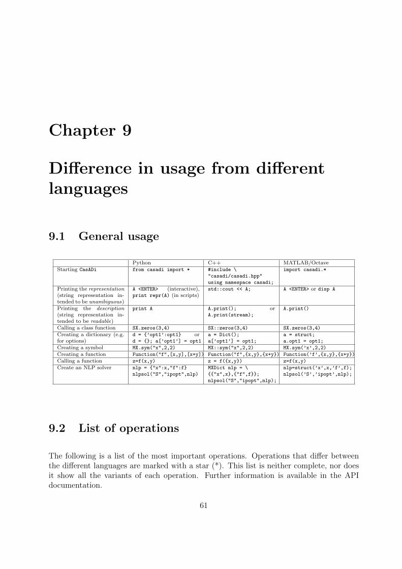
Chapter 9

Difference in usage from differentlanguages

9.1 General usage

Python C++ MATLAB/OctaveStarting CasADi from casadi import * #include \

"casadi/casadi.hpp"

using namespace casadi;

import casadi.*

Printing the representation(string representation in-tended to be unambiguous)

A <ENTER> (interactive),print repr(A) (in scripts)

std::cout << A; A <ENTER> or disp A

Printing the description(string representation in-tended to be readable)

print A A.print(); orA.print(stream);

A.print()

Calling a class function SX.zeros(3,4) SX::zeros(3,4) SX.zeros(3,4)

Creating a dictionary (e.g.for options)

d = {’opt1’:opt1} ord = {}; a[’opt1’] = opt1

a = Dict();

a[’opt1’] = opt1;

a = struct;

a.opt1 = opt1;

Creating a symbol MX.sym("x",2,2) MX::sym("x",2,2) MX.sym(’x’,2,2)

Creating a function Function("f",[x,y],[x+y]) Function("f",{x,y},{x+y}) Function(’f’,{x,y},{x+y})

Calling a function z=f(x,y) z = f({x,y}) z=f(x,y)

Create an NLP solver nlp = {"x":x,"f":f}

nlpsol("S","ipopt",nlp)

MXDict nlp = \

{{"x",x},{"f",f}};

nlpsol("S","ipopt",nlp);

nlp=struct(’x’,x,’f’,f);

nlpsol(’S’,’ipopt’,nlp);

9.2 List of operations

The following is a list of the most important operations. Operations that differ betweenthe different languages are marked with a star (*). This list is neither complete, nor doesit show all the variants of each operation. Further information is available in the APIdocumentation.

61

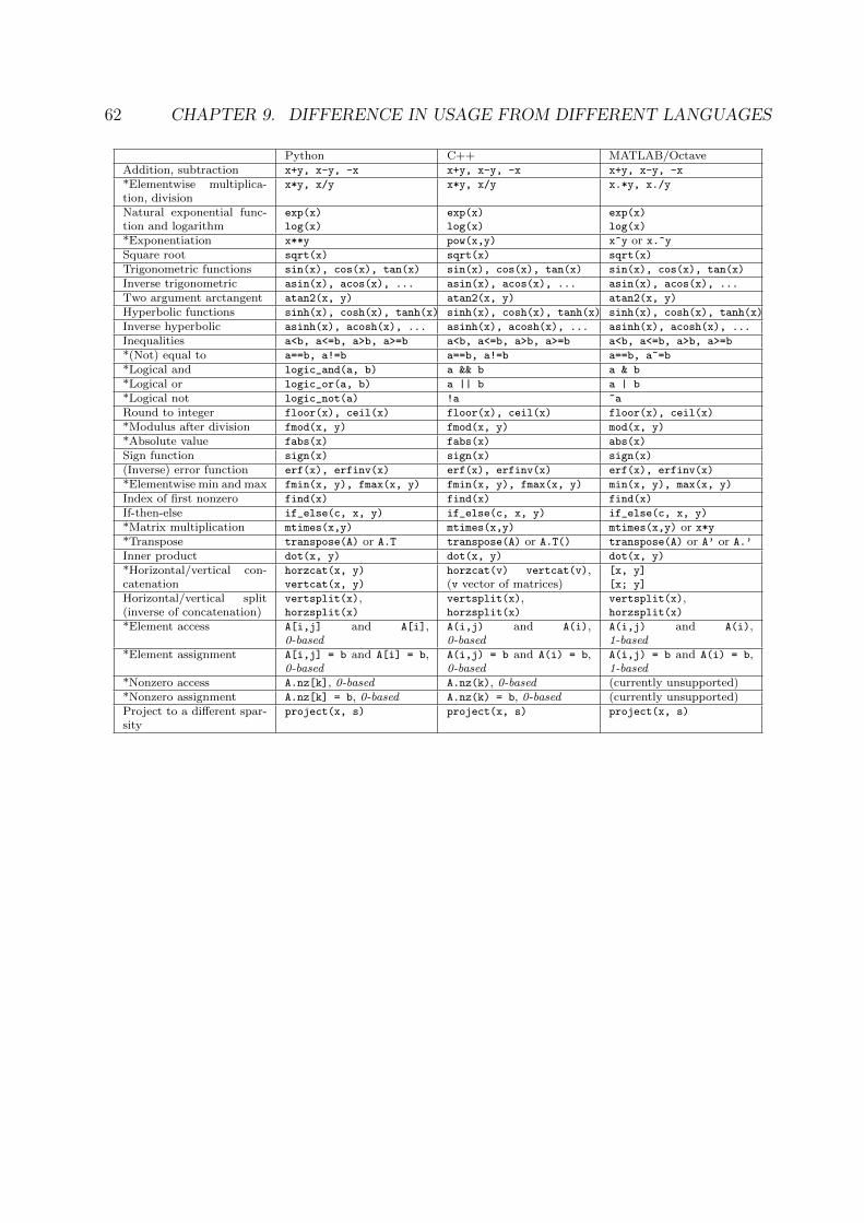
62 CHAPTER 9. DIFFERENCE IN USAGE FROM DIFFERENT LANGUAGES

Python C++ MATLAB/OctaveAddition, subtraction x+y, x-y, -x x+y, x-y, -x x+y, x-y, -x

*Elementwise multiplica-tion, division

x*y, x/y x*y, x/y x.*y, x./y

Natural exponential func-tion and logarithm

exp(x)

log(x)

exp(x)

log(x)

exp(x)

log(x)

*Exponentiation x**y pow(x,y) x^y or x.^y

Square root sqrt(x) sqrt(x) sqrt(x)

Trigonometric functions sin(x), cos(x), tan(x) sin(x), cos(x), tan(x) sin(x), cos(x), tan(x)

Inverse trigonometric asin(x), acos(x), ... asin(x), acos(x), ... asin(x), acos(x), ...

Two argument arctangent atan2(x, y) atan2(x, y) atan2(x, y)

Hyperbolic functions sinh(x), cosh(x), tanh(x) sinh(x), cosh(x), tanh(x) sinh(x), cosh(x), tanh(x)

Inverse hyperbolic asinh(x), acosh(x), ... asinh(x), acosh(x), ... asinh(x), acosh(x), ...

Inequalities a<b, a<=b, a>b, a>=b a<b, a<=b, a>b, a>=b a<b, a<=b, a>b, a>=b

*(Not) equal to a==b, a!=b a==b, a!=b a==b, a~=b

*Logical and logic_and(a, b) a && b a & b

*Logical or logic_or(a, b) a || b a | b

*Logical not logic_not(a) !a ~a

Round to integer floor(x), ceil(x) floor(x), ceil(x) floor(x), ceil(x)

*Modulus after division fmod(x, y) fmod(x, y) mod(x, y)

*Absolute value fabs(x) fabs(x) abs(x)

Sign function sign(x) sign(x) sign(x)

(Inverse) error function erf(x), erfinv(x) erf(x), erfinv(x) erf(x), erfinv(x)

*Elementwise min and max fmin(x, y), fmax(x, y) fmin(x, y), fmax(x, y) min(x, y), max(x, y)

Index of first nonzero find(x) find(x) find(x)

If-then-else if_else(c, x, y) if_else(c, x, y) if_else(c, x, y)

*Matrix multiplication mtimes(x,y) mtimes(x,y) mtimes(x,y) or x*y

*Transpose transpose(A) or A.T transpose(A) or A.T() transpose(A) or A’ or A.’

Inner product dot(x, y) dot(x, y) dot(x, y)

*Horizontal/vertical con-catenation

horzcat(x, y)

vertcat(x, y)

horzcat(v) vertcat(v),(v vector of matrices)

[x, y]

[x; y]

Horizontal/vertical split(inverse of concatenation)

vertsplit(x),horzsplit(x)



*Element access A[i,j] and A[i],0-based

A(i,j) and A(i),0-based

A(i,j) and A(i),1-based

*Element assignment A[i,j] = b and A[i] = b,0-based

A(i,j) = b and A(i) = b,0-based

A(i,j) = b and A(i) = b,1-based

*Nonzero access A.nz[k], 0-based A.nz(k), 0-based (currently unsupported)*Nonzero assignment A.nz[k] = b, 0-based A.nz(k) = b, 0-based (currently unsupported)Project to a different spar-sity

project(x, s) project(x, s) project(x, s)

Date post:	17-Feb-2019
Category:	Documents
Upload:	buique
View:	251 times
Download:	0 times

User Documentation for CasADi...

Documents