István János Tóth 1 - Miklós Hajdu 2 Intensity of Competition, Corruption Risks and Price Distortion in the Hungarian Public Procurement – 2009-2016 Working Paper Series CRCB-WP/2017:2 December 2017 - Budapest 1 Corruption Research Center Budapest, [email protected]2 Corruption Research Center Budapest, [email protected]
Transcript
István János Tóth1 - Miklós Hajdu2
Intensity of Competition, Corruption Risks and Price Distortion in
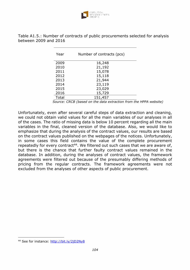
The report examines Hungarian public procurement data in the period between 2009 and 2016. Data from 151,457 contracts were used for the analysis, which focuses on
information about the intensity of competition, price distortion and corruption risks. We analysed price distortion using Benford’s law. We also studied the performance of EU-funded projects from these viewpoints. The results show that 2016 was a very special
year from the aspect of Hungarian public procurement, as there was a major decrease in the number of contracts and an extremely low proportion of EU-funded public
procurement. The findings also provide evidence for the presence of price distortion based on different approaches during the period under examination. Finally, employing several methods, we estimated the volume of direct social loss due to corruption.
According to the results, the aggregate amount of estimated direct social loss reached at least 2.1–3.3 trillion forints (6.7–10.6 billion euros) and came to 15–24% of total
public procurement spending in the 2009–2016 period. Based on the results, we point out that EU funding has perverse effects on public procurement in Hungary: it has aided in reducing the intensity of competition and increasing both the level of corruption risk
and the weight of price distortion, and it has generated the growth of estimated direct social loss due to weak competition and a high level of corruption risk during the period.
JEL classification: D22, D72, H57, L13
Keywords: public procurement, intensity of competition, price distortion, corruption risk,
social loss, empirical analysis Hungary
3
The Corruption Research Center Budapest was created in November 2013 in response
to the growing need for independent research on corruption and quality of government in Hungary. Hence, the Center was established as a non-partisan research institute
independent of governments, political parties or special interest groups. The aims of the Center are to systematically explore the causes, characteristics, and consequences
of low quality of government, corruption, and regulatory failure using an inter-disciplinary approach. The Center also aims to help citizens to hold governments accountable through the use of empirical evidence.
Intensity of Competition, Corruption Risks and Price Distortion in the
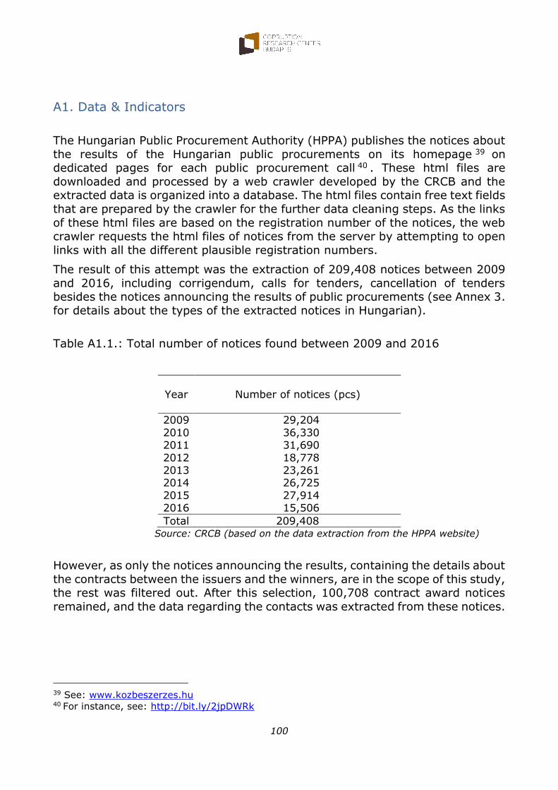
A1. Data & Indicators .................................................................................. 100
A2. Some specific problems and errors of the official data management of the Hungarian public procurement ...................................................................... 109
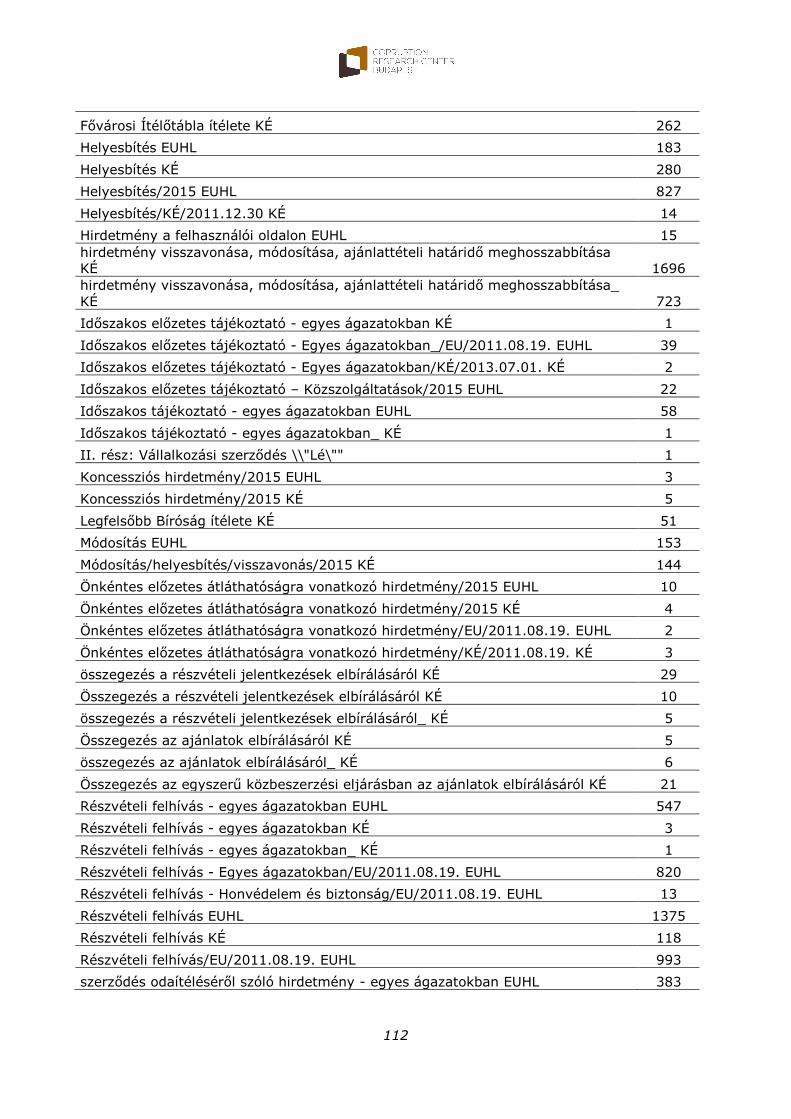
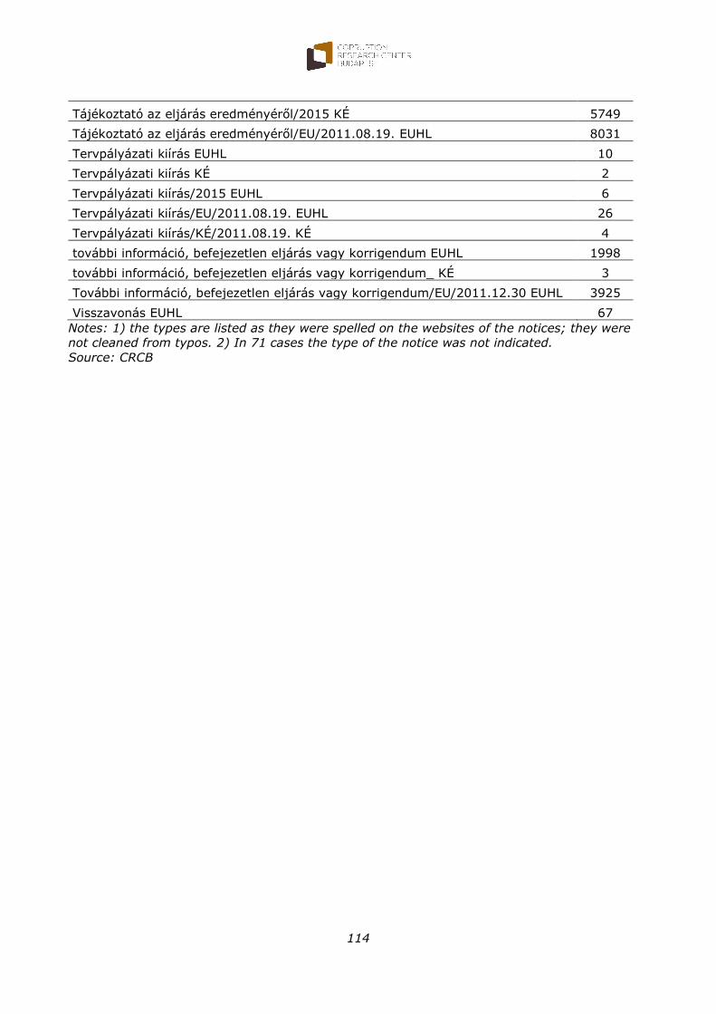
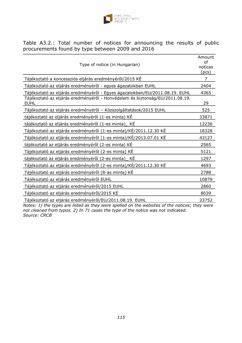
A3. Extracted types of notices from the website of the HPPA ............................ 111
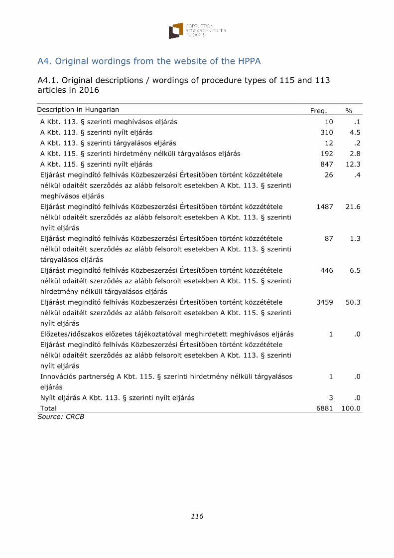
A4. Original wordings from the website of the HPPA ........................................ 116
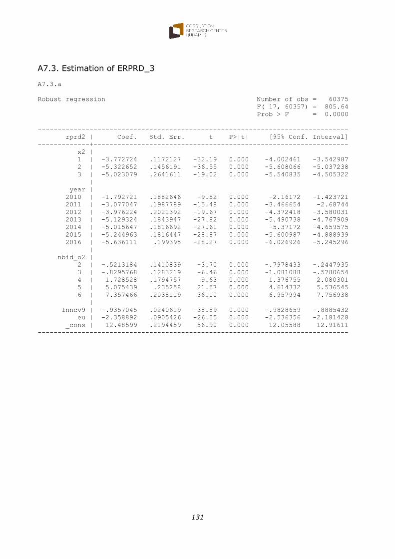
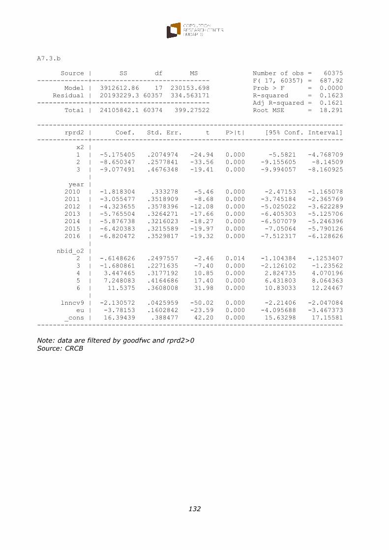
A7. Estimations of Direct Social Loss ............................................................. 129
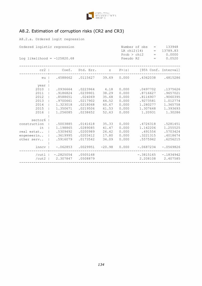
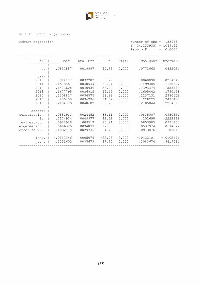
A8. Analysis of EU effects on intensity of competition, level of corruption risks, price distortion and rate of estimated direct social loss ............................................ 133
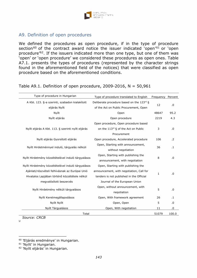
A9. Definition of open procedures ................................................................. 143
5
Executive Summary
The report examines Hungarian public procurement data in the period
between 2009 and 2016. Data on 151,457 contracts were used for the analysis. The report focuses on information about the intensity of
competition, price distortion and corruption risks. We also analyse the performance of EU-funded projects from these viewpoints. The results
provide evidence of price distortion based on several different approaches during the period under examination. Based on observations derived from
contract data, we also estimate the magnitude of estimated direct social loss due to corruption risk and weak completion.
In 2016, there was a major decrease in the number of contracts (it was about two-thirds of the 2015 volume), which occurred due to a sharp drop
in the quantity of EU-funded contracts, although the aggregate sum of net contract values for 2016 barely changed compared to 2015.
It was anticipated that the new Public Procurement Act (Act CXLIII of 2015
on Public Procurement) would generate an upturn in the intensity of competition (although some provisions of the Act could potentially trigger
the opposite result). We expected an increase in the proportion of contracts with an estimated value and in the number of contracts per
procedure and a decrease in the frequency of public tenders with unannounced negotiated procedures. These expectations were confirmed
by our empirical analysis.
Between 2015 and 2016, the share of contracts with one, two or three
bidders fell in total number of contracts, and there was a rise in the proportion of contracts with four, five or more than five bidders. These
changes stem mostly from tenders where the contract value did not exceed the EU threshold. The sudden growth in the share of contracts with
four bidders may be a consequence of the new public procurement law, as it mandated a larger number of participants (i.e. at least four) in certain
negotiated procedures.
During the 2009–2015 period, the intensity of competition (an index based on the number of bids) decreased, while it increased slightly in 2016.
Between 2009 and 2015, the intensity of competition tended to be lower for EU-financed public procurement compared to public procurement
financed from national sources. However, this difference disappeared by 2016.
The Transparency Index (TI) of public procurement provides information on the way in which tenders were issued (with or without an
announcement). The level of TI in 2015–2016 remained far below the 2009–2010 level. Since 2011, EU-funded tenders were characterised by
significantly lower TI values in each year than non-EU-funded ones. The detailed analysis shows that the level of TI was significantly weaker in
6
2016 than in 2015, when we control for EU funding, the size of contract
and sector.
Besides transparency, the occurrence of single-bidder contracts is another important indicator of corruption risks. The share of tenders with a single
bid (i.e. non-competitive tenders) decreased between 2015 and 2016; however, it remained high (28% of all tenders). In 2016, the decline in
the share of single-bidder contracts was less prevalent for tenders financed by EU grants compared to non-EU-funded ones. In international
comparison on the basis of the TED database, the share of tenders with only a single-bidder is notably high in Hungary, varying between 25% and
33% in 2006–2015. During the same period, the share of non-competitive tenders did not exceed 12% in the old EU member states (for instance,
Denmark, France, the Netherlands, Germany and Sweden). This is a clear sign that Hungarian public procurement tenders are strongly affected by
corruption risks.
Based on the composite corruption risk indicator, which combines
information on transparency, single bidding and an element of price
distortion, an upward trend in corruption risks can be observed between 2009 and 2015. The average value of the corruption risk indicator fell
slightly in 2016 but remained at a relatively high level, and it was higher for EU-funded tenders than for non-EU-funded ones between 2010 and
2016.
We examined the amount of money spent on public tenders marked by
the highest level of corruption risk. We defined this aggregate value taking into account tenders where the value of the corruption risk indicator was
1, and then we aggregated the contract value of these tenders. The results show that in 2016 the aggregate value of tenders with the highest level of
corruption risk moved up compared to those in 2014–2015 and the relative share of these tenders in total value of all tenders grew from 30% to
around 44% in 2016.
The concept of price distortion/overpricing is related to corruption. We
consider the former as an outcome of a corrupt situation. In the case of a
corrupt tender, the contract price includes the economic rent generated by corruption in addition to the market price. As a consequence, price
setting within corrupt tenders must be fundamentally different from that of tenders involving competition. We interpret price distortion as a sign of
a non-zero level of corruption risk. We use three methods to detect this phenomenon: we analyse (i) rounded data in contract prices; (ii) the
observed distribution of first digits of net contract price against distribution of first digits predicted by the Benford’s law; and, finally, (iii) the drop in
contract prices compared to the estimated value of tenders (i.e. the price estimated by the issuer and published in the call for tenders).
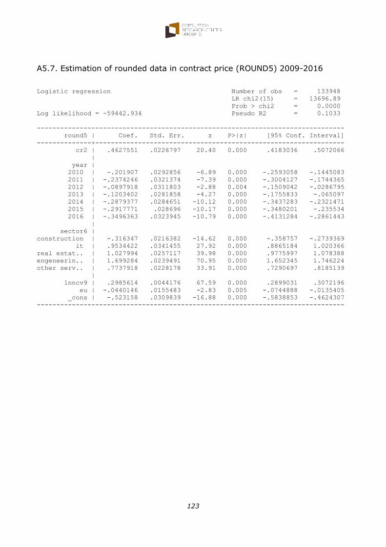
The indicators of rounded prices show a decreasing trend in price distortion in the last three years. However, the value of the rounded price indicators
7
remained very high: more than 60% of contract prices were rounded in
Hungarian public procurement.
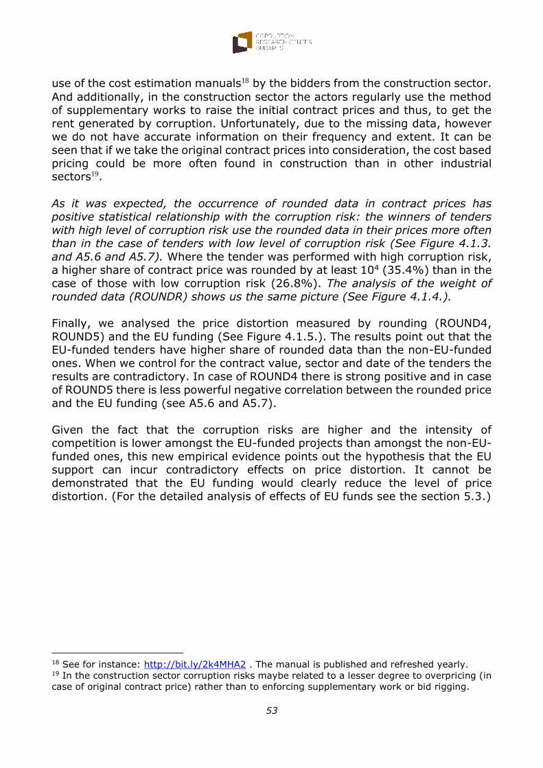
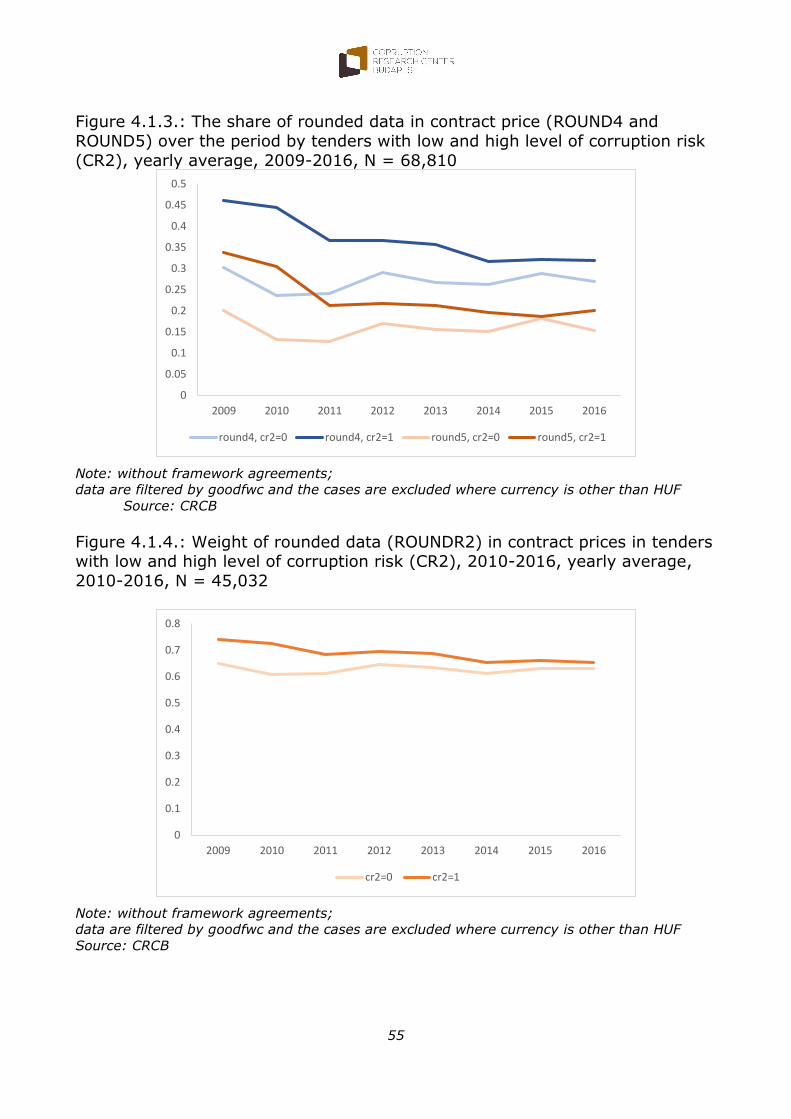
There is a weak positive statistical relationship between the occurrence of rounded data in contract prices and the level of corruption risk. Winners
of tenders with a high level of corruption risk use rounded data in their prices more often than winners of tenders with low corruption risk. Where
the tender was implemented with high corruption risk, a higher share of the contract price was rounded by at least 10,000 (35%) than in the case
of those with low corruption risk (27%).
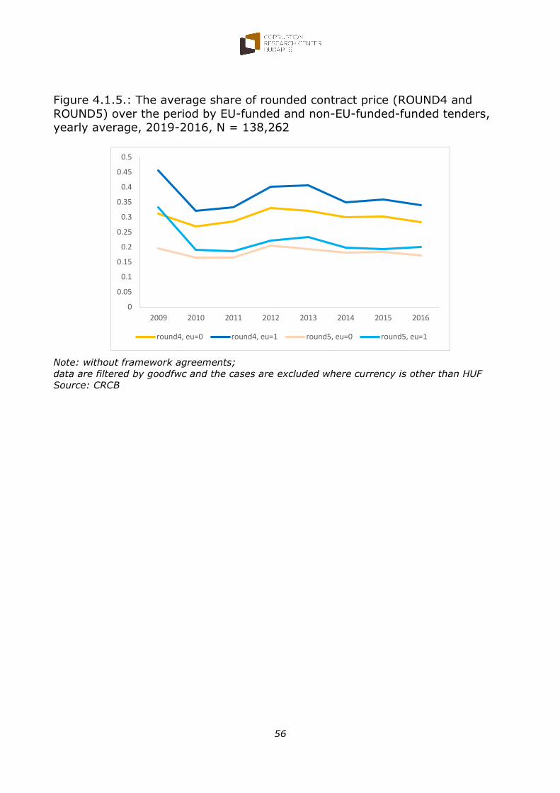
We analysed price distortion measured by rounding in EU-funded projects.
The results show that EU funding has a contradictory effect on price distortion when we control for the contract value, sector and date of
tenders. Given that corruption risks are higher and the intensity of competition is lower for EU-funded projects than for non-EU-funded ones,
this new empirical evidence on price distortion points out the hypothesis that the that EU support can produce contradictory effects in Hungary.
Spending of EU funds is thus associated with higher corruption risks,
weaker intensity of competition and it cannot be demonstrated that the EU funding would clearly reduce the level of price distortion.
We also analysed price distortion in terms of the distribution of the first digits in contract prices based on Benford’s law. This analysis indicates
that contract prices in Hungarian public procurement tenders fit the theoretical distribution well when the 2009–2016 period is examined as a
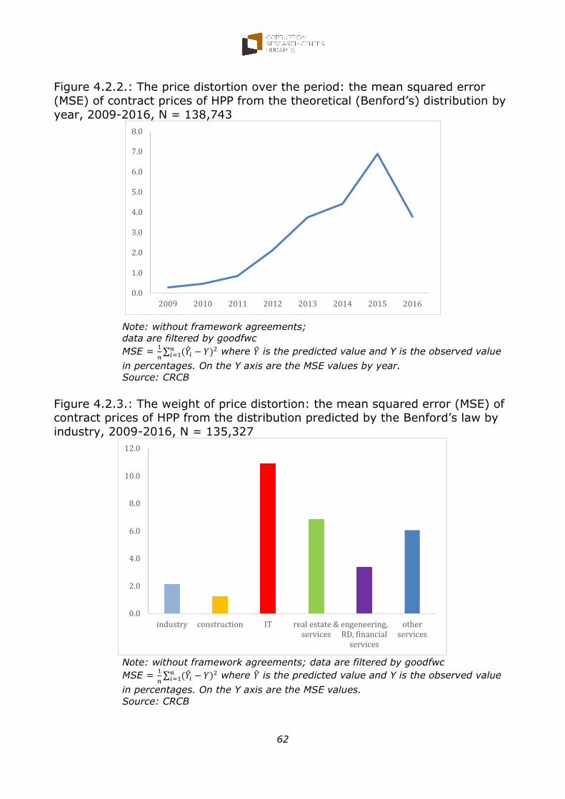
whole. However, there are significant differences in price distortion across years: price distortion rose in the first seven years based on this measure.
While contract prices fit the theoretical distribution well in 2009 and 2010, the magnitude of price distortion became significant thereafter. This
observation indicates a rising frequency of overpricing, pointing to weakening competition and growing corruption risks. In 2016, the degree
of price distortion fell compared to the peak level in 2015, but remained significantly high.
The construction sector and industry appear to display the lowest level of
price distortion vis-à-vis Benford’s distribution, while the IT sector is characterised by the highest. The high level of price distortion in the IT
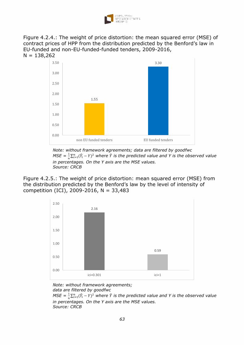
sector is probably related to the large share of heterogeneous and specific goods and services in this sector. The results again show that EU-funded
tenders are more affected by price distortion than nationally funded ones.
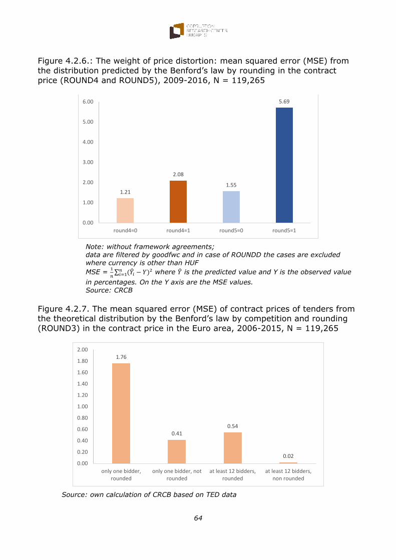
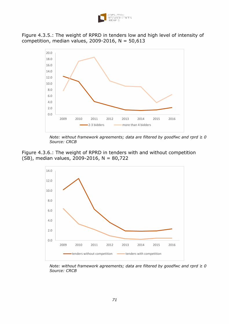
Our findings highlight that the strength of price distortion falls as intensity
of competition becomes stronger. The prices in public procurement contracts are remarkably distorted when there is no competition (i.e.
single-bid tenders). There is also a positive correlation between the two independent indicators of price distortion: the level of price distortion
measured by Benford’s law is significantly higher for contracts with rounded prices than for those with non-rounded contract prices.
8
There is a clear indication that the strength of price distortion as captured
by Benford’s law increases significantly with the growth of corruption risk.
This result supports our hypothesis on the positive relationship between corruption risks and price distortion. Price distortion over the entire period
under examination is closely linked to tenders marked by high corruption risks as measured by our composite risk indicators. Our analysis suggests
that the significant increase in price distortion in the 2009–2015 period was driven by the effect of EU-funded projects.
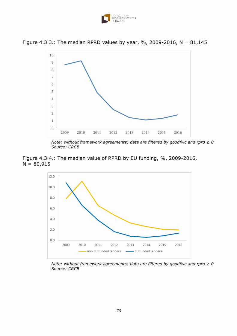
The magnitude of the price drop in the actual contract price relative to the estimated value can be regarded as a proxy measure for the intensity of
competition. The core assumption behind this is that increased competition between bidders will produce more intense price competition, which should
lead to lower prices in the end. Thus, the greater magnitude of the price drop points to a higher level of competition intensity in public tenders,
while a low or zero price drop represents low intensity or lack of competition.
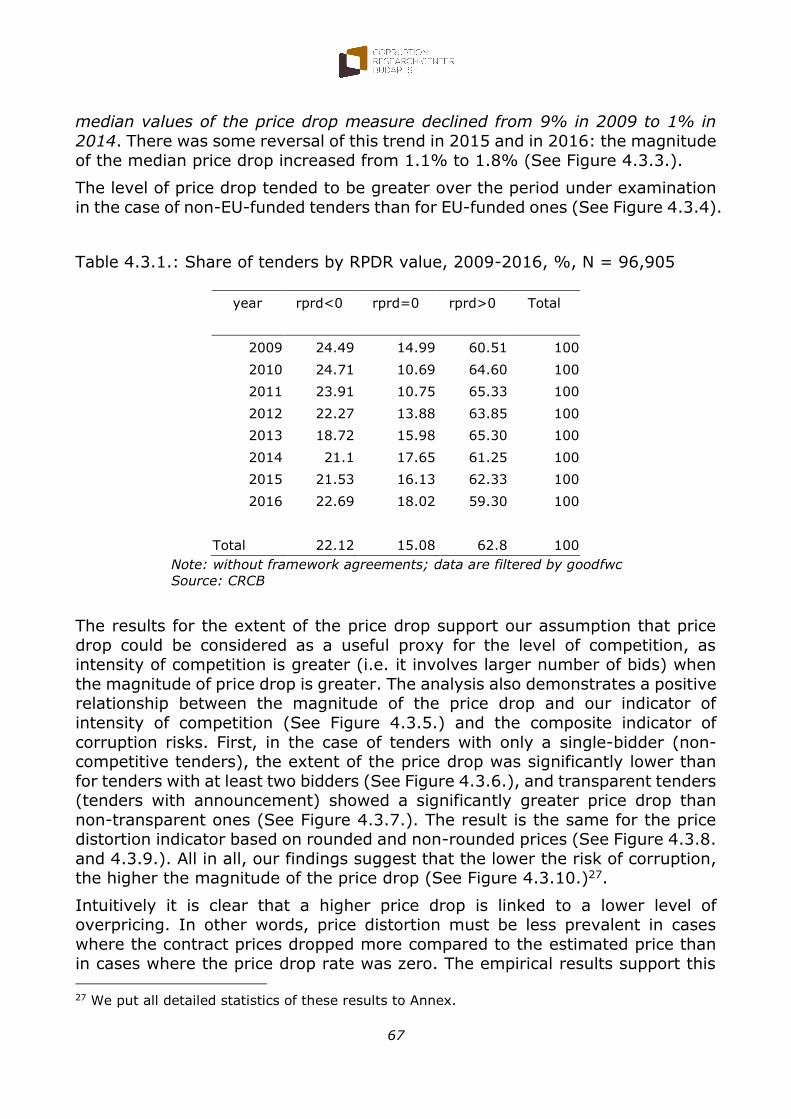
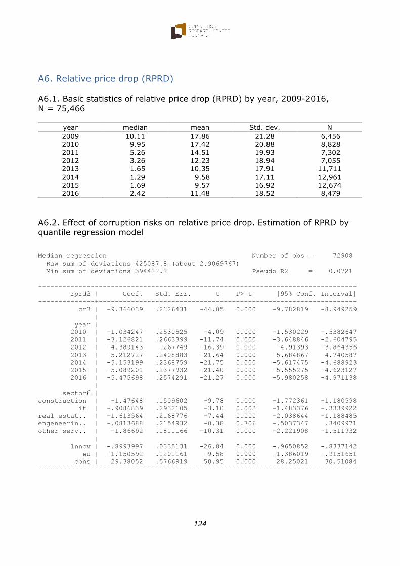
The price drop weakened significantly over the period under examination:
the median values of the price drop measure declined from 9% in 2009–2010 to 1% in 2014–2015. There was some reversal of this trend in 2015
and 2016: the magnitude of the median price drop increased from 1.3% to 1.8%.
The extent of the price drop tended to be greater over the period under examination for non-EU-funded tenders than for EU-funded ones.
The results for the extent of the price drop support our assumption that the price drop could be considered as a useful proxy for the level of
competition, as intensity of competition is greater (i.e. it involves larger number of bids) when the magnitude of the price drop is greater. The
analysis also demonstrates a positive relationship between the magnitude of the price drop and our composite indicator of corruption risks. First, in
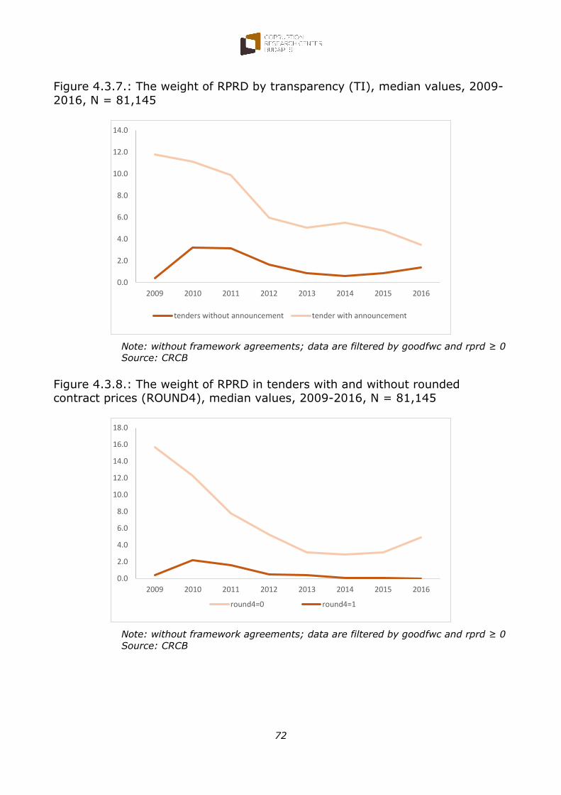
the case of tenders with only a single-bidder (non-competitive tenders), the extent of the price drop was significantly lower than for tenders with
at least two bidders, and transparent tenders (tenders with announcement)
showed a significantly greater price drop than non-transparent ones. The result is the same for the price distortion indicator based on rounded and
non-rounded prices. All in all, our findings suggest that the lower the risk of corruption, the higher the magnitude of the price drop.
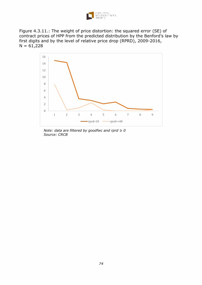
A higher price drop is linked to a lower level of overpricing. In other words, price distortion must be less prevalent in cases where contract prices
dropped more compared to the estimated price than in cases where the price drop rate was zero. The empirical results support this insight: with
regard to the magnitude of squared errors from distribution of first digits of contract price predicted by the Benford’s law, the data do show that
prices of tenders with a large price drop conform more significantly to Benford’s law than those with a small price drop. We concluded that the
9
magnitude of the price drop provides us with information not only on the
level of intensity of competition, but also on corruption risks and the
existence of price distortion.
Looking at the pattern of the price drop indicator over time, we found that
the extent of the price drop decreased significantly between 2009 and 2015, but there was some reversal of this trend in 2016. The extent of the
price drop was greater for non-EU-funded tenders than for EU-funded ones, and tenders above the EU threshold value were marked by a significantly
greater price drop than those below this threshold.
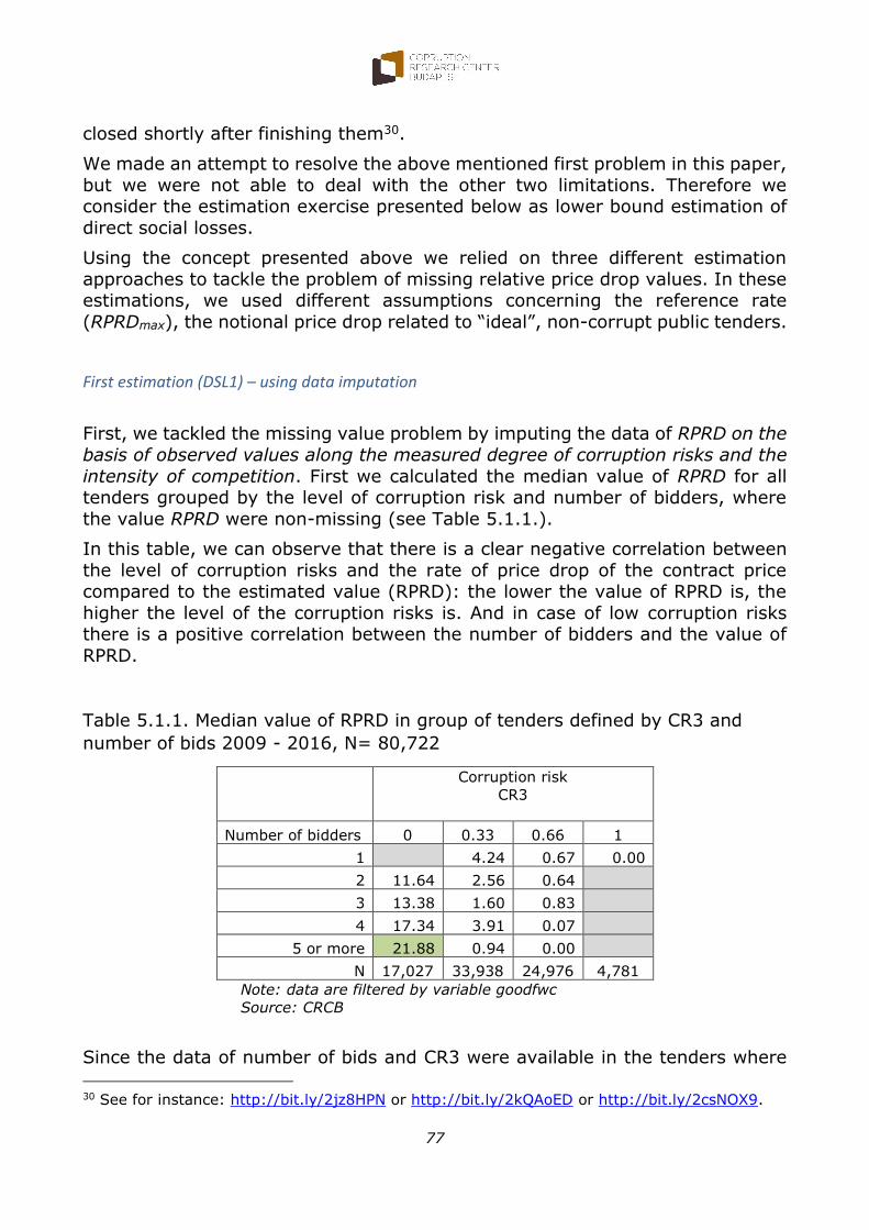
The estimated direct social loss of tenders with high corruption risks and
a low level of intensity of competition takes the form of rent, which occurs when payments are made above competitive market prices. The high
corruption risk and/or low level of intensity of competition in public procurement are regularly and closely associated with political favouritism
and rent seeking. In the report, we present one approach to estimating direct social loss in public tenders due to high corruption risk and low
competition. First, we evaluate the differences in average contract prices
between public tenders with and without corruption risks. Second, we assess differences between estimated and actual contract prices.
Although our estimation results on direct social loss due to high corruption risks and a low level of intensity of competition can be considered as lower
bound estimates, they demonstrate an astonishingly high direct social loss in Hungarian public procurement. Based on the measured gap between
the net estimated contract value and the actual contract price, the analysis shows a very high level of estimated direct social loss: 15–24% in total
contract value in the 2009–2016 period. According to our findings, the aggregate amount of estimated direct social loss reached at least 2.1–3.3
trillion forints (6.7–10.6 billion euros) during this period.
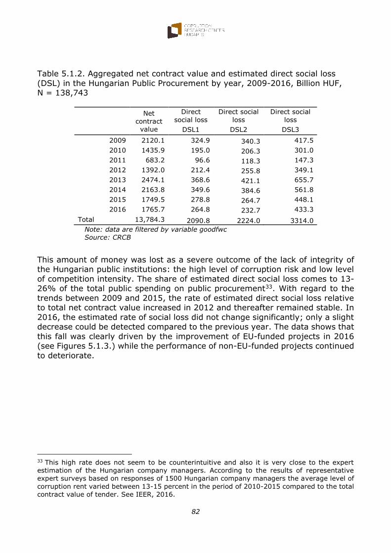
With regard to the trends between 2009 and 2015, the rate of estimated
direct social loss relative to total net contract value increased in 2012 and thereafter remained stable. In 2016, the estimated rate of social loss did
not change significantly; only a slight decrease could be detected
compared to the previous year.
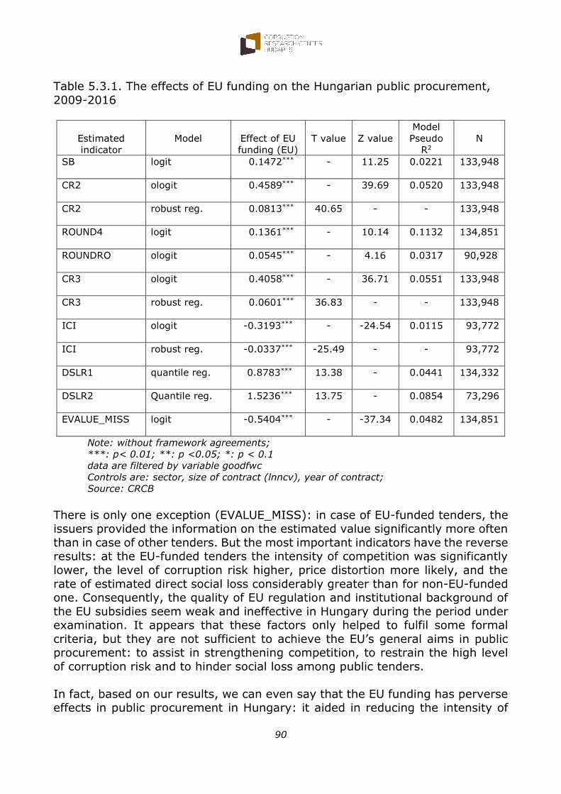
In the case of EU-funded tenders, the intensity of competition was
significantly lower, the level of corruption risk higher, price distortion more likely, and the rate of estimated direct social loss considerably greater than
for non-EU-funded ones. Consequently, the quality of EU regulation and the institutional background of EU subsidies seem weak and ineffective in
Hungary during the period under examination. It appears that these factors only helped to fulfil some formal criteria, but they are not sufficient
to achieve the EU’s general aims in public procurement: to assist in strengthening competition, to restrain the high level of corruption risk and
to hinder social loss among public tenders. In fact, based on our results, we can even say that EU funding has perverse effects in public
10
procurement in Hungary: it aided in reducing the intensity of competition
and increasing both the level of corruption risk and the weight of price
distortion, it spurred the growth of estimated direct social loss due to weak competition, and to high level of corruption risk during the period.
11
Introduction
The goal of the report
The goal of this report3 is twofold. On the one hand, we would like to present
analytic tools to examine the phenomenon of corruption in public procurement; and on the other hand, the report illustrates the use of the presented tools
through the empirical analysis of the Hungarian public procurement data in the period of 2009-2016. In the report we analyse the Hungarian public procurement
in terms of intensity of competition, corruption risks, and price distortion.
Frist, we are using a unique dataset of the Hungarian public procurement created by the CRCB’s staff4. The CRCB downloaded 209,408 notices and 176,886
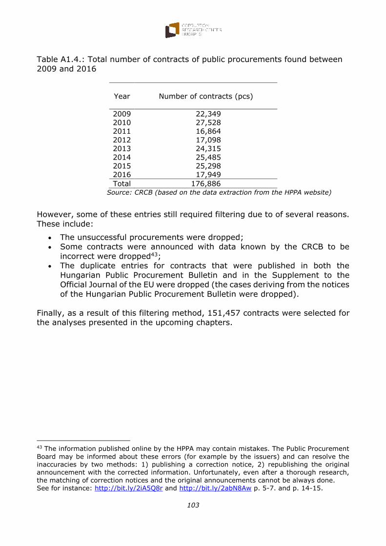
procedures’ data from the Hungarian Public Procurement Authority’s web page from the period of 2009-2016 and then these data were cleansed and arranged
into a complete database. Data about all the awarded contracts and about all those published in the Public Procurement Bulletin during the whole year of 2016
from January 1st to December 31st were accounted for in the report and analysed. Our primary aim was to examine what changes took place in the
Hungarian Public Procurement process in 2016. The openness of the procedure,
the number of tenders without competition, the level of corruption risk and the volume of price distortion were scrutinized. The analysis is mainly descriptive,
but, where possible, the analysis takes a more in-depth approach.
An analysis of this kind can be significant in at least two ways, that are related to each other. On the one hand, the actors’ (institutions with calls for tender and
bidder companies) behavioural change is studied with respect to corruption risk, intensity of competition and price distortion with descriptive statistical tools. On
the other hand, only the data from public procurement contracts can provide answers regarding the impact from changes in the public procurement legal
system (e.g. the modification of the public procurement law) had on the public 3 We would like to express our sincere thanks to Katalin Goldstein, Samuel Markson, Balázs
Molnár, Attila Székely and Magda József for their valuable help during the database building and
preparation of this report. We also would like to thank to Katalin Andor, Iván Csaba, the public
procurement experts of the Hungarian government, and the participants of the meeting
organized by ECFIN on 22 June 2017 for their invaluable comments and suggestions on this
report. 4. In the framework of the ongoing research program of CRCB, we are restoring, cleaning the
data of the Hungarian public procurement in the period of 1998-2017 to build a comprehensive,
well-structured database for the future empirical research on competition, corruption of public
tenders. Neither the Hungarian authorities (including the Hungarian Public Procurement
Authority) nor the Hungarian taxpayers have such a database. See other research programs on
this topic: the CEU Microdata (http://bit.ly/2ARyGzg) and the Digiwhist project
procurement actors’ behaviour, and furthermore the extent to which the
regulatory changes increased the intensity of competition or lowered the chance
of corruption in public procurement.
Our analysis focuses on providing an answer to the first question, while at the same time it wishes to contribute to the more in-depth studies that target the
economic analysis of the effects of governmental regulatory decisions.
In the first part of the report the changes in the number and in the value of public procurement that happened in 2016 are to be dealt with. After that the
intensity of competition, corruption risk and price distortion will be analysed. In the next part, there will be an attempt to have an estimation on the direct social
losses that are linked to a low competition intensity and overpricing. Finally the assessment concerning the year of 2016 will be summed up. The description the
database and indicators used for this specific study can be found in the Annex besides some supplemental information that may help in understanding the
outcomes.
Brief conceptual framework
During the report we use two general concepts: corruption and competition. For simplicity we include the several forms of collusion (cartels, bid rigging) into the
concept of corruption, because these activities also hurt the rules of competition.
We interpret the corrupt activity of players of public tenders in the frame of principal-agent model (Rose-Ackermann, 2006; Lambsdorff, 2007). In the case
of public procurement, the concept of corruption and competition can basically be described by three different phenomena: (i) a public tender is conducted in
accordance with the rules of the competition, thus there is no corruption here. Or (ii) the tender is corrupt, thus there is no competition here; (iii) or at the
given public tender there is competition and corruption as well. It is possible that the corrupt offers of actors competed with each other to obtain the tender.
During the analysis, we use elementary and composite indicators which are based on information derived from official publications (announcements and
contract awards) of Hungarian public procurement5. In this report we focus on only information of six different factors6:
1. the date of public tender;
2. the type of procedure (especially: whether it was a call for tenders or
5 We have extracted all our data for the webpage of the Hungarian Public Procurement
Authority. See: http://bit.ly/2r1sIHM 6 We omit to deal with other important factors of public tenders as the time elapsed between
the invitation to tender and the tender’s submission (in calendar days or working days); the
name of issuer; the type of issuer; the address of issuer; the name of winner; the address of
winner; the names of other bidders; and finally the address of other bidders.
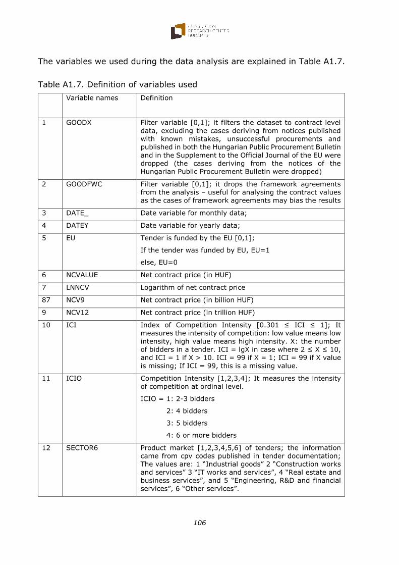
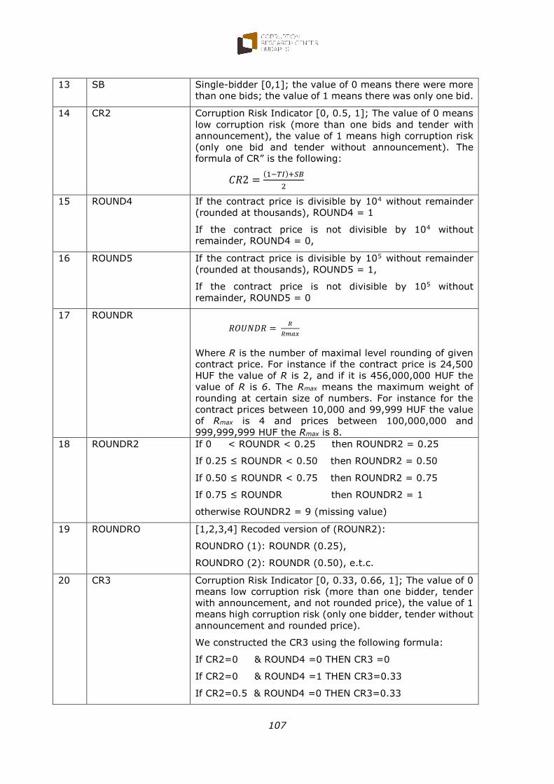
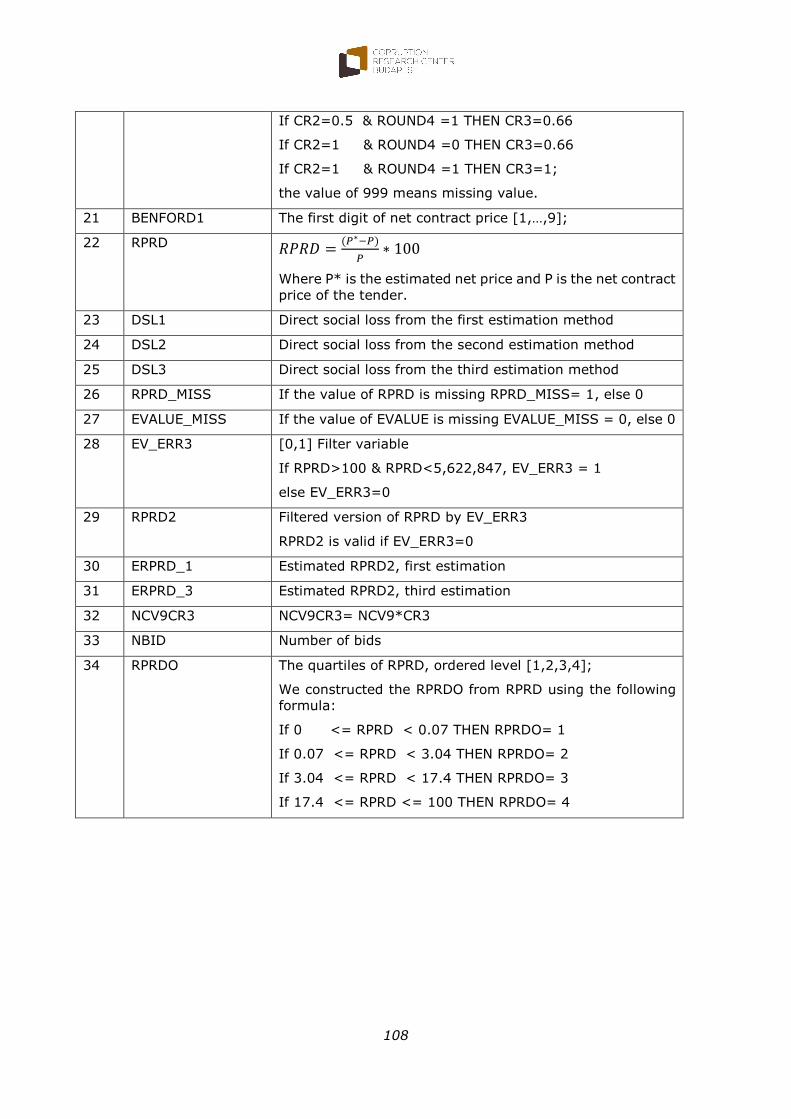
For the purpose of analysis we constructed several elementary and composite indicators that indirectly serve to measure the various aspects of competition
and corruption. These are the following (for the precise definitions see the Annex 1.7.):
1. Transparency index (TI) [0,1], dummy variable;
2. Single-bidder (SB); [0,1], dummy variable;
3. ICI: index of competition intensity;
4. Rounded contract price (ROUND4); its value is 1, if the net contract
value is rounded by 104; and 0, else;
5. Rounded contract price (ROUND5); its value is 1, if the net contract
value is rounded by 105; and 0, else;
6. Relative weight of rounding (ROUNDR2); the winner price includes what degree of rounding [0.25, 0.5, 0.75, 1], ordered variable;
7. BENFORD1: the first digit test of net contract price, categorical variable;
8. RPRD: the rate of price drop; net contract price compared to the
estimated value;
9. Indicator of corruption risk (CR2) with two components (TI and SB)
[0, 0.5, 1]; ordered variable;
10. Indicator of corruption risk (CR3) with three components (TI, SB, and
ROUND4) [0, 0.33, 0.66, 1]; ordered variable;
The listed and above identified indicators are used to measure three operationalized concepts (i) corruption risks, (ii) price distortion, and (iii),
intensity of competition.
Corruption risks relate to the existence of conditions of corruption. We assume
that actors who want to behave in a corrupt way will create the conditions which
meet the planned corrupt transaction. Corruption risks measure the extent to which effective conditions for corruption have been created.
Corruption risks should be measured primarily by indicators that can already be seen before or during the public procurement process (e.g. type of public tender
or the number of bids submitted), but information on the assessment of
14
corruption risks can also be used to relate to the outcome of procedure used.
For instance, these may include information on the contract prices. From these
information, it can be deduced how effective the conditions were for corruption existing in the given public tender. Accordingly, these indicators cannot be used
as classical “red flags”. With regard to the ongoing procedures, their use cannot provide predictions of which public procurement is more likely to be threatened
by corruption. But with the help of these indicators, after the completion of public tenders, it is possible to analyse which group or types of tenders, winners or
issuers had the highest or lowest risk of corruption.
This analytical strategy can also be useful in tackling corruption: it raises the
light of the type of public tenders that needs to be taken to cover the risk of corruption; what sort of public procurement might be more likely to be
threatened by corrupt transactions. But they also help answer the question about the actual impact of modification of public procurement rules / laws on the
corruption risks of public tenders.
Another important concept for which we would like to propose measurement
tools is price distortion. In this report we only look at the distortion of contract
prices, and we do not deal with the price distortion at estimated value. Analysing the price distortion, we rely essentially on the methods developed in fraud
analysis and forensic accounting. Among the tools recommended by these researches (Nigrini, 2012; Miller, 2015; Kossovsky, 2015), only two will be used
in this report: (i) the last-two digit test; (ii) and the first digit test and these two test will take only for net contract prices. The former is a powerful test for
number invention (Nigrini, 2012) and the latter is a general and basic tool for the detection of distortive behaviour of price setting actors, in our case, the
winners and in certain special cases, the issuers.
According to fraud detection research, rounded values point out to the presence
of distortion. It is worth observing the rounded values (prices) in the context of intensity of competition and corruption risks and examine the relationships
amongst them. In this analysis we use four indicators to measure the rounded values: the ROUND4, ROUND5 and ROUNDR2 indicators.
We believe that the strength of corruption risks and intensity of competition in
the public procurement market are closely related to the price distortion: in a corrupt situation, the winning price is rather an invented price, which should
contain economic rent related to corruption and thus the price should be higher than the market price. In the case of a corrupt public tender, the winners are
likely to invent their prices without any cost based, or market based analysis and therefore they are more likely to apply invented prices accordingly.
The other indicator comes from the first digit test of Benford's distribution (BENFORD1). In a natural market environment - such as when public tenders
are driven by rules of competition, winning prices are not accompanied by any external (non-competitive) effects. In that case, the prices of public tenders
behave like market prices. The purchase of goods by the issuers and the responsive bid prices of the bidders (the companies participating in the public
15
procurement competition) are also generated as a result of the natural processes
i.e. competition, that are determined by the rules of competition. Thus, the first
digits of the winning prices should then be Benford's distribution: that is, if most of the public procurement is conducted on a competitive basis, we expect the
first digit of the contract price to be distributed to Benford’s Law. Completely other outcome could be expected in a corrupt situation: the price setting at these
tenders does not follow the natural, competitive rules, because the behaviour of the corrupt actors (issuers and/or bidders), as one of possible form of rent-
seeking behaviour, tends to generate corruption benefit. Accordingly, at tenders with high corruption risks and low level of intensity of competition we expect
higher price distortion, i.e. the distribution of first digits of contract price has the highest difference from the predicted, Benford’s distribution.
The third concept is the intensity of competition. It means at what level of competitive intensity the public tenders are conducted. If, for example, at a
given tender there were 6-7 bids, it is considered to be a higher competition intensity than if there were only 2-3 bids competing. The intensity of competition
is measured on the one hand by the index of competition intensity (ICI, ICIO).
On the other hand, another indicator also includes the aspect of how much the contracted price of the winner has been lower than the estimated price by the
issuer (estimated value). For this, we observe the difference between the contact price and the estimated value relative to the contact price (RPRD). The
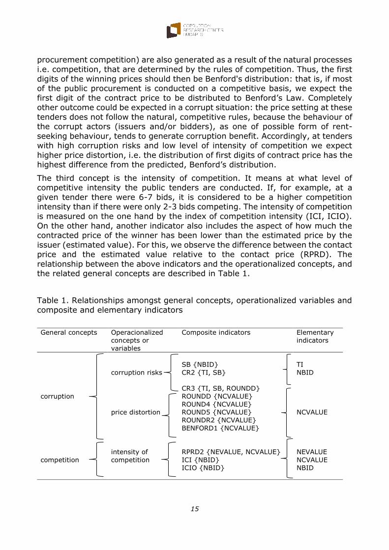
relationship between the above indicators and the operationalized concepts, and the related general concepts are described in Table 1.
Table 1. Relationships amongst general concepts, operationalized variables and
composite and elementary indicators
General concepts Operacionalized
concepts or
variables
Composite indicators Elementary
indicators
corruption
corruption risks
SB {NBID}
CR2 {TI, SB}
TI
NBID
CR3 {TI, SB, ROUNDD}
price distortion
ROUNDD {NCVALUE}
NCVALUE
ROUND4 {NCVALUE}
ROUND5 {NCVALUE}
ROUNDR2 {NCVALUE}
BENFORD1 {NCVALUE}
competition
intensity of
competition
RPRD2 {NEVALUE, NCVALUE}
NEVALUE
ICI {NBID} NCVALUE
ICIO {NBID}
NBID
16
1. What happened in 2016?
It seems that 2016 was a very special year from the aspect of the Hungarian
public procurement, as there was a major decrease in the number of contracts (it was about the two-third of the 2015 volume) and the ratio of public
procurements with EU-fund was extremely low. The most important tendencies are the following:
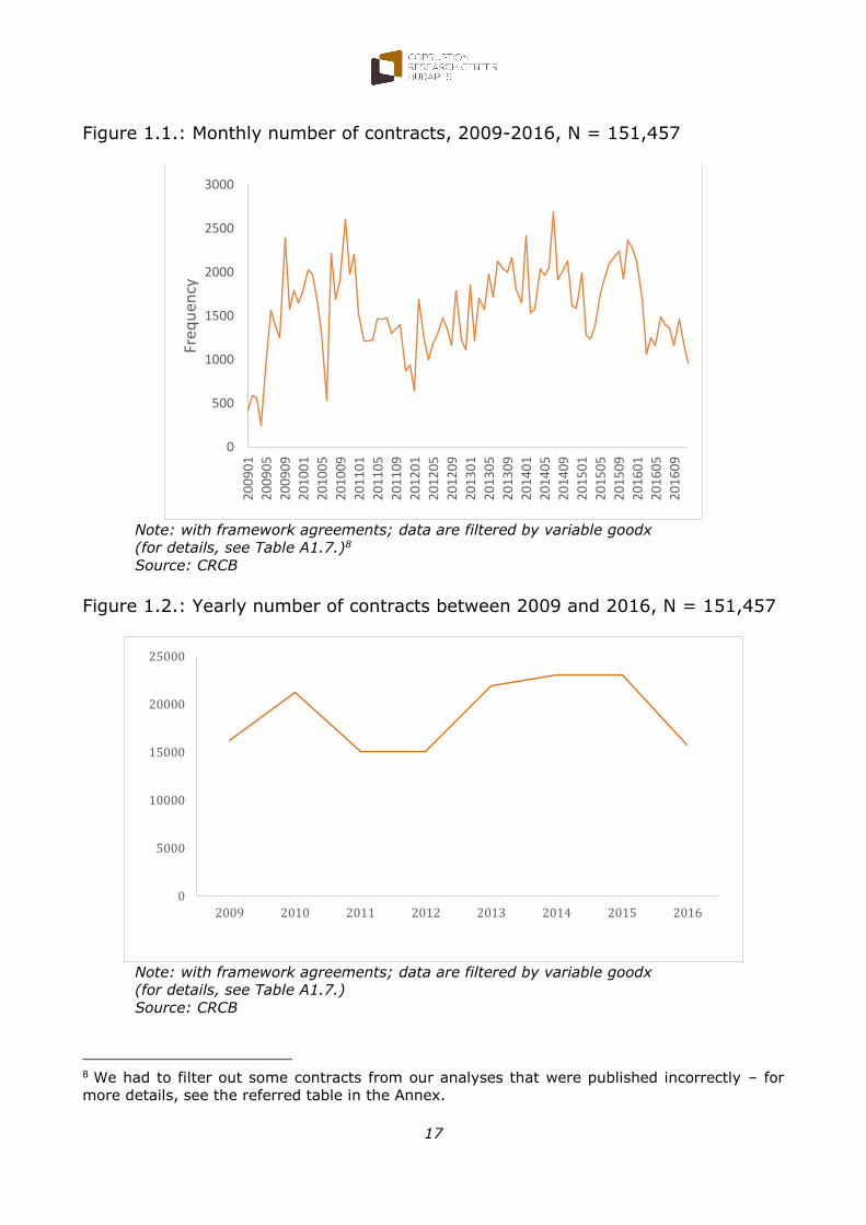
Regarding the monthly number of contracts, a major decrease occurred
during the first quarter of 2016 (see Fig. 1.1.).
The total number of contracts in 2016 was significantly less than it was between 2013 and 2015 (see Fig. 1.2.).
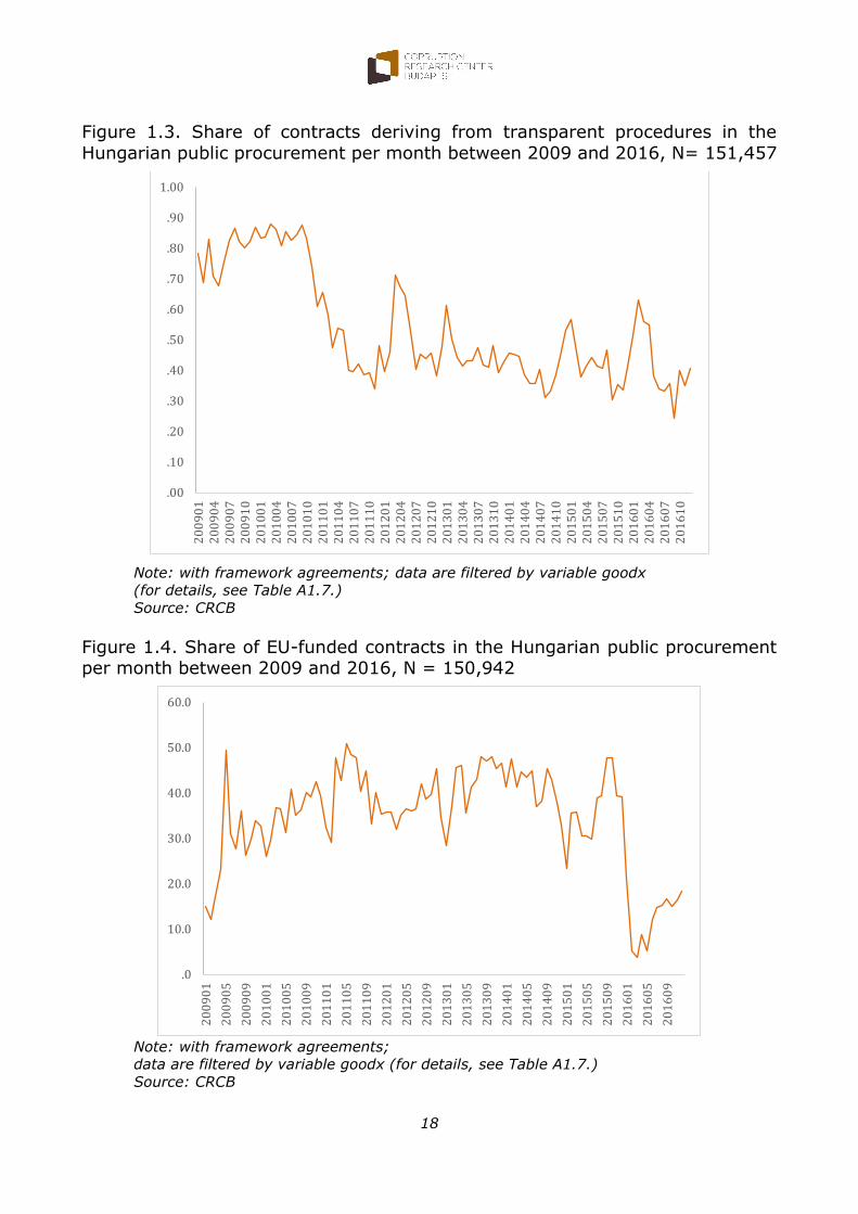
The share of EU-funded contracts fell dramatically in the first month of
2016 (see Fig. 1.4.).
During 2016, the share of EU-funded contracts was far less than it was
between 2009 and 2015 (see Fig. 1.5.).
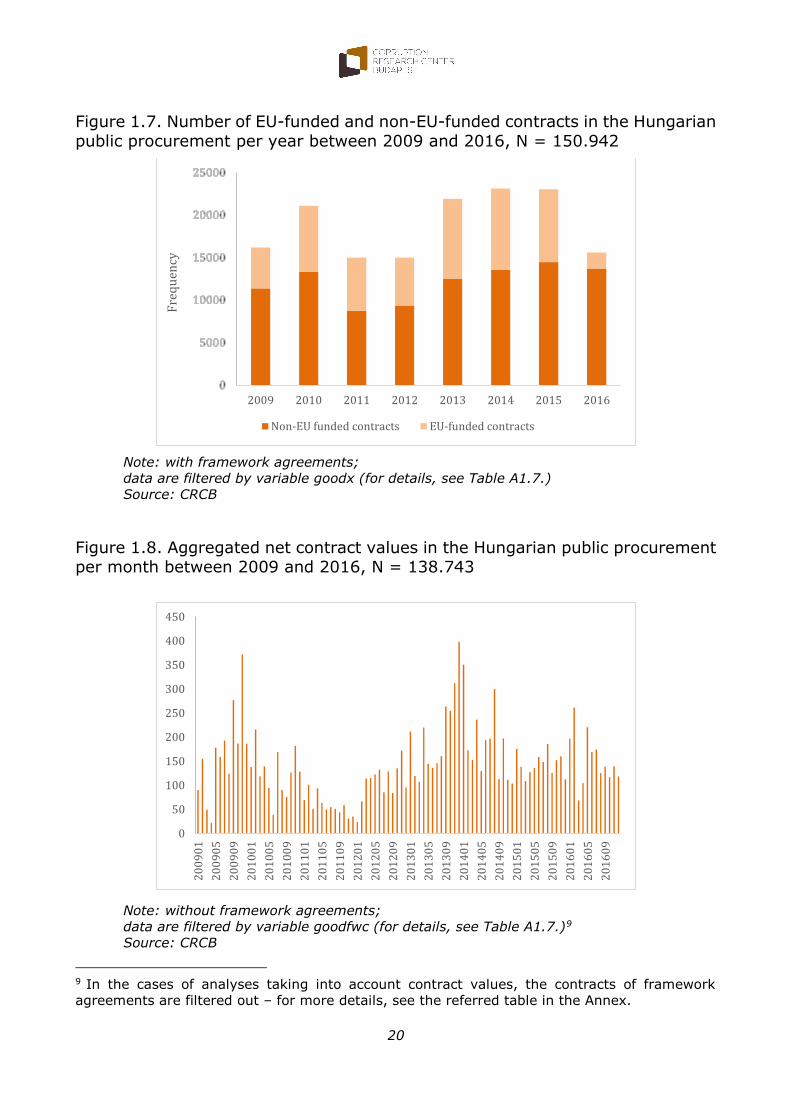
While the number of contracts without EU-funds show only minor changes between 2013 and 2016, there was a drop in EU-funded contracts in 2016
what resulted in the major decrease in the overall number of contacts (see Fig. 1.7.).
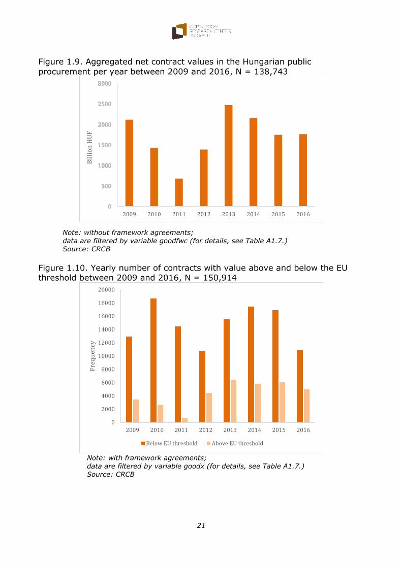
The aggregated sum of the net contract values7 for 2016 barely changed
in comparison to 2015 (see Fig. 1.9.); besides that the number of the contracts decreased, the average of net contract value increased to 128
million HUF from 84 million HUF between 2015 and 2016.
7 The framework agreements are excluded from this analysis – for details, see A1.
17
Figure 1.1.: Monthly number of contracts, 2009-2016, N = 151,457
Note: with framework agreements; data are filtered by variable goodx
(for details, see Table A1.7.)8
Source: CRCB
Figure 1.2.: Yearly number of contracts between 2009 and 2016, N = 151,457
Note: with framework agreements; data are filtered by variable goodx
(for details, see Table A1.7.)
Source: CRCB
8 We had to filter out some contracts from our analyses that were published incorrectly – for
more details, see the referred table in the Annex.
0
500
1000
1500
2000
2500
3000
20
09
01
20
09
05
20
09
09
20
10
01
20
10
05
20
10
09
20
11
01
20
11
05
20
11
09
20
12
01
20
12
05
20
12
09
20
13
01
20
13
05
20
13
09
20
14
01
20
14
05
20
14
09
20
15
01
20
15
05
20
15
09
20
16
01
20
16
05
20
16
09
Freq
uen
cy
0
5000
10000
15000
20000
25000
2009 2010 2011 2012 2013 2014 2015 2016
18
Figure 1.3. Share of contracts deriving from transparent procedures in the
Hungarian public procurement per month between 2009 and 2016, N= 151,457
Note: with framework agreements; data are filtered by variable goodx
(for details, see Table A1.7.)
Source: CRCB
Figure 1.4. Share of EU-funded contracts in the Hungarian public procurement per month between 2009 and 2016, N = 150,942
Note: with framework agreements;
data are filtered by variable goodx (for details, see Table A1.7.)
Source: CRCB
.00
.10
.20
.30
.40
.50
.60
.70
.80
.90
1.002
00
90
12
00
90
42
00
90
72
00
91
02
01
00
12
01
00
42
01
00
72
01
01
02
01
10
12
01
10
42
01
10
72
01
11
02
01
20
12
01
20
42
01
20
72
01
21
02
01
30
12
01
30
42
01
30
72
01
31
02
01
40
12
01
40
42
01
40
72
01
41
02
01
50
12
01
50
42
01
50
72
01
51
02
01
60
12
01
60
42
01
60
72
01
61
0
.0
10.0
20.0
30.0
40.0
50.0
60.0
20
09
01
20
09
05
20
09
09
20
10
01
20
10
05
20
10
09
20
11
01
20
11
05
20
11
09
20
12
01
20
12
05
20
12
09
20
13
01
20
13
05
20
13
09
20
14
01
20
14
05
20
14
09
20
15
01
20
15
05
20
15
09
20
16
01
20
16
05
20
16
09
19
Figure 1.5. Share of EU-funded procedures contracts in the Hungarian public
procurement per year between 2009 and 2016, N = 150,942
Note: with framework agreements;
data are filtered by variable goodx (for details, see Table A1.7.)
Source: CRCB
Figure 1.6. Number of EU-funded and non-EU-funded contracts in the Hungarian
public procurement per month between 2009 and 2016, N = 150.942
Note: with framework agreements;
data are filtered by variable goodx (for details, see Table A1.7.)
Source: CRCB
0%
10%
20%
30%
40%
50%
60%
70%
80%
90%
100%
2009 2010 2011 2012 2013 2014 2015 2016
20
09
01
20
09
05
20
09
09
20
10
01
20
10
05
20
10
09
20
11
01
20
11
05
20
11
09
20
12
01
20
12
05
20
12
09
20
13
01
20
13
05
20
13
09
20
14
01
20
14
05
20
14
09
20
15
01
20
15
05
20
15
09
20
16
01
20
16
05
20
16
09
Fre
qu
ency
Non-EU funded contracts EU-funded contracts
20
Figure 1.7. Number of EU-funded and non-EU-funded contracts in the Hungarian
public procurement per year between 2009 and 2016, N = 150.942
Note: with framework agreements;
data are filtered by variable goodx (for details, see Table A1.7.)
Source: CRCB
Figure 1.8. Aggregated net contract values in the Hungarian public procurement per month between 2009 and 2016, N = 138.743
Note: without framework agreements;
data are filtered by variable goodfwc (for details, see Table A1.7.)9
Source: CRCB
9 In the cases of analyses taking into account contract values, the contracts of framework
agreements are filtered out – for more details, see the referred table in the Annex.
2009 2010 2011 2012 2013 2014 2015 2016
Fre
qu
ency
Non-EU funded contracts EU-funded contracts
0
50
100
150
200
250
300
350
400
450
20
09
01
20
09
05
20
09
09
20
10
01
20
10
05
20
10
09
20
11
01
20
11
05
20
11
09
20
12
01
20
12
05
20
12
09
20
13
01
20
13
05
20
13
09
20
14
01
20
14
05
20
14
09
20
15
01
20
15
05
20
15
09
20
16
01
20
16
05
20
16
09
21
Figure 1.9. Aggregated net contract values in the Hungarian public
procurement per year between 2009 and 2016, N = 138,743
Note: without framework agreements;
data are filtered by variable goodfwc (for details, see Table A1.7.)
Source: CRCB
Figure 1.10. Yearly number of contracts with value above and below the EU threshold between 2009 and 2016, N = 150,914
Note: with framework agreements;
data are filtered by variable goodx (for details, see Table A1.7.)
Source: CRCB
2009 2010 2011 2012 2013 2014 2015 2016
Bil
lio
n H
UF
0
2000
4000
6000
8000
10000
12000
14000
16000
18000
20000
2009 2010 2011 2012 2013 2014 2015 2016
Fre
qu
ency
Below EU threshold Above EU threshold
22
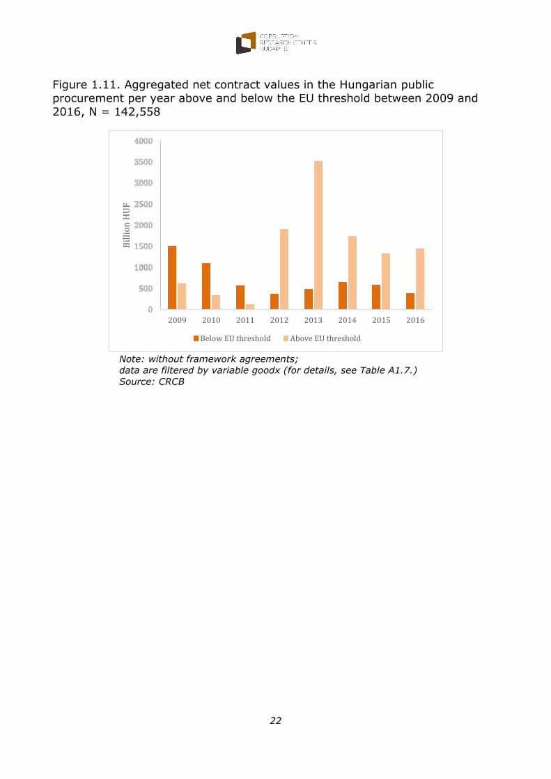
Figure 1.11. Aggregated net contract values in the Hungarian public
procurement per year above and below the EU threshold between 2009 and
2016, N = 142,558
Note: without framework agreements;
data are filtered by variable goodx (for details, see Table A1.7.)
Source: CRCB
2009 2010 2011 2012 2013 2014 2015 2016
Bil
lio
n H
UF
Below EU threshold Above EU threshold
23
2. Intensity of competition
In this section, first we analyse the evolution of number of bidders by years then
we construct an indicator which summarize the information on intensity of competition using the number of bidders at public tenders. The number of
bidders can be regarded as an indicator of competition.
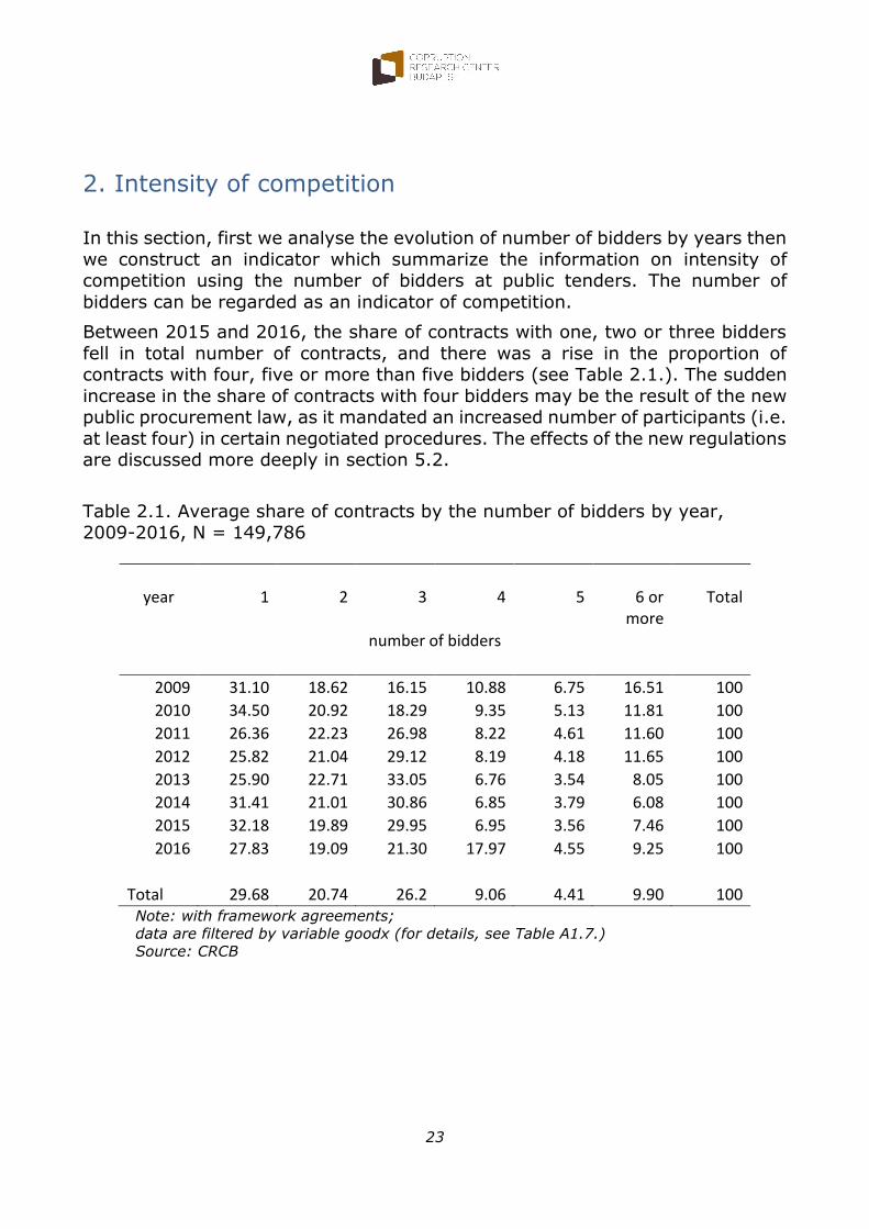
Between 2015 and 2016, the share of contracts with one, two or three bidders
fell in total number of contracts, and there was a rise in the proportion of contracts with four, five or more than five bidders (see Table 2.1.). The sudden
increase in the share of contracts with four bidders may be the result of the new public procurement law, as it mandated an increased number of participants (i.e.
at least four) in certain negotiated procedures. The effects of the new regulations are discussed more deeply in section 5.2.
Table 2.1. Average share of contracts by the number of bidders by year, 2009-2016, N = 149,786
year 1 2 3 4 5
6 or more
Total
number of bidders
2009 31.10 18.62 16.15 10.88 6.75 16.51 100
2010 34.50 20.92 18.29 9.35 5.13 11.81 100
2011 26.36 22.23 26.98 8.22 4.61 11.60 100
2012 25.82 21.04 29.12 8.19 4.18 11.65 100
2013 25.90 22.71 33.05 6.76 3.54 8.05 100
2014 31.41 21.01 30.86 6.85 3.79 6.08 100
2015 32.18 19.89 29.95 6.95 3.56 7.46 100
2016 27.83 19.09 21.30 17.97 4.55 9.25 100
Total 29.68 20.74 26.2 9.06 4.41 9.90 100 Note: with framework agreements;
data are filtered by variable goodx (for details, see Table A1.7.)
Source: CRCB
24
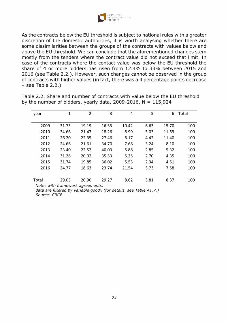
As the contracts below the EU threshold is subject to national rules with a greater
discretion of the domestic authorities, it is worth analysing whether there are
some dissimilarities between the groups of the contracts with values below and above the EU threshold. We can conclude that the aforementioned changes stem
mostly from the tenders where the contract value did not exceed that limit. In case of the contracts where the contact value was below the EU threshold the
share of 4 or more bidders has risen from 12.4% to 33% between 2015 and 2016 (see Table 2.2.). However, such changes cannot be observed in the group
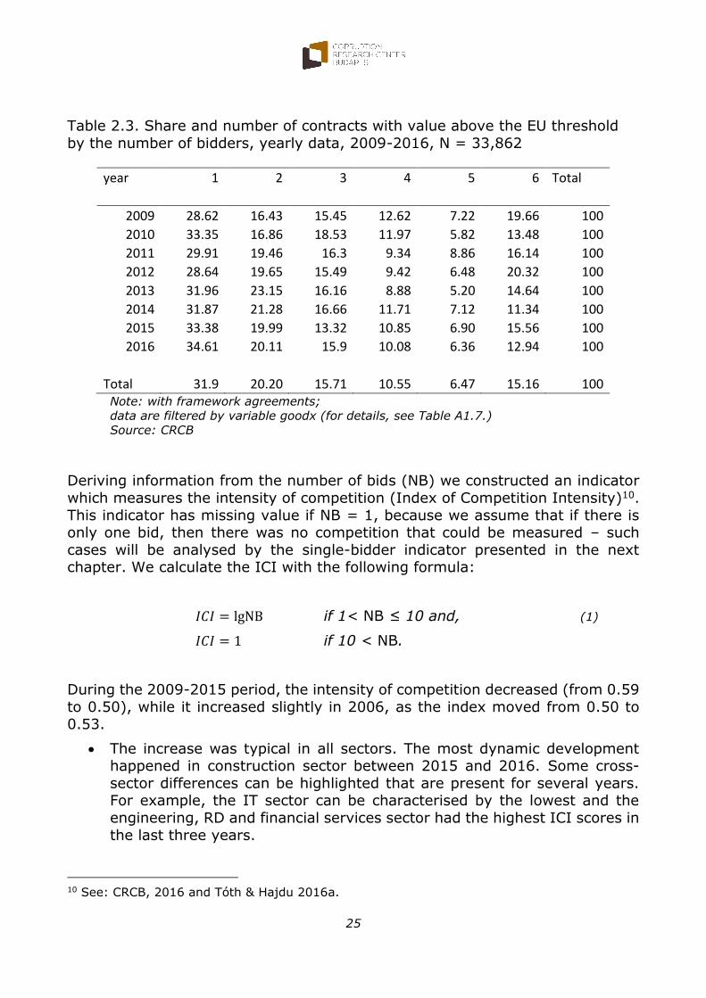
of contracts with higher values (in fact, there was a 4 percentage points decrease – see Table 2.2.).
Table 2.2. Share and number of contracts with value below the EU threshold
by the number of bidders, yearly data, 2009-2016, N = 115,924
year 1 2 3 4 5 6 Total
2009 31.73 19.19 16.33 10.42 6.63 15.70 100
2010 34.66 21.47 18.26 8.99 5.03 11.59 100
2011 26.20 22.35 27.46 8.17 4.42 11.40 100
2012 24.66 21.61 34.70 7.68 3.24 8.10 100
2013 23.40 22.52 40.03 5.88 2.85 5.32 100
2014 31.26 20.92 35.53 5.25 2.70 4.35 100
2015 31.74 19.85 36.02 5.53 2.34 4.51 100
2016 24.77 18.63 23.74 21.54 3.73 7.58 100
Total 29.03 20.90 29.27 8.62 3.81 8.37 100 Note: with framework agreements;
data are filtered by variable goodx (for details, see Table A1.7.)
Source: CRCB
25
Table 2.3. Share and number of contracts with value above the EU threshold
by the number of bidders, yearly data, 2009-2016, N = 33,862
year 1 2 3 4 5 6 Total
2009 28.62 16.43 15.45 12.62 7.22 19.66 100
2010 33.35 16.86 18.53 11.97 5.82 13.48 100
2011 29.91 19.46 16.3 9.34 8.86 16.14 100
2012 28.64 19.65 15.49 9.42 6.48 20.32 100
2013 31.96 23.15 16.16 8.88 5.20 14.64 100
2014 31.87 21.28 16.66 11.71 7.12 11.34 100
2015 33.38 19.99 13.32 10.85 6.90 15.56 100
2016 34.61 20.11 15.9 10.08 6.36 12.94 100
Total 31.9 20.20 15.71 10.55 6.47 15.16 100 Note: with framework agreements;
data are filtered by variable goodx (for details, see Table A1.7.)
Source: CRCB
Deriving information from the number of bids (NB) we constructed an indicator
which measures the intensity of competition (Index of Competition Intensity)10.
This indicator has missing value if NB = 1, because we assume that if there is only one bid, then there was no competition that could be measured – such
cases will be analysed by the single-bidder indicator presented in the next chapter. We calculate the ICI with the following formula:
𝐼𝐶𝐼 = lgNB if 1< NB ≤ 10 and, (1)
𝐼𝐶𝐼 = 1 if 10 < NB.
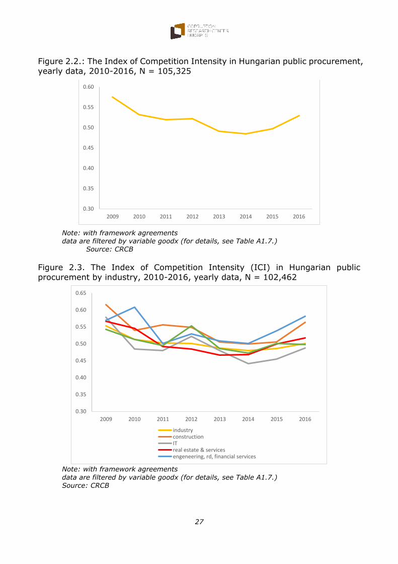
During the 2009-2015 period, the intensity of competition decreased (from 0.59
to 0.50), while it increased slightly in 2006, as the index moved from 0.50 to 0.53.
The increase was typical in all sectors. The most dynamic development happened in construction sector between 2015 and 2016. Some cross-
sector differences can be highlighted that are present for several years. For example, the IT sector can be characterised by the lowest and the
engineering, RD and financial services sector had the highest ICI scores in
the last three years.
10 See: CRCB, 2016 and Tóth & Hajdu 2016a.
26
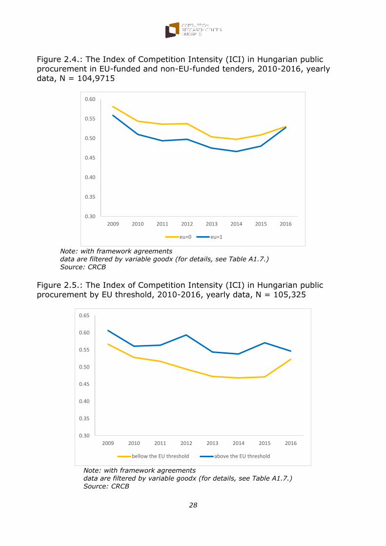
Between 2009 and 2015, the intensity of competition tended to be lower
for the EU-financed public procurement compared to public procurement
financed from national sources by about 0.03-0.04 units of the ICI. This difference disappeared by 2016, as the value of ICI was 0.53 in both of
the groups.
We can find the same feature when we classify the tenders according to the EU threshold. While between 2009 and 2015 the intensity of
competition of public tenders below the EU threshold tended to be lower than the tenders above the threshold (in 2015, there was 0.1 unit
difference between the two groups), this difference almost had vanished in 2016. In 2016, the intensity of corruption of tenders below the EU
threshold increased from 0.47 to 0.52, while the ones above the threshold decreased from 0.57 to 0.55; therefore, the two groups reached almost
the same level of intensity of competition by 2016.
Figure 2.1.: The Index of Competition Intensity in Hungarian public procurement,
monthly data, 2009-2016, N = 105,325
Note: with framework agreements
data are filtered by variable goodx (for details, see Table A1.7.)
Source: CRCB
0.30
0.35
0.40
0.45
0.50
0.55
0.60
0.65
0.70
0.75
20
09
01
20
09
05
20
09
09
20
10
01
20
10
05
20
10
09
20
11
01
20
11
05
20
11
09
20
12
01
20
12
05
20
12
09
20
13
01
20
13
05
20
13
09
20
14
01
20
14
05
20
14
09
20
15
01
20
15
05
20
15
09
20
16
01
20
16
05
20
16
09
27
Figure 2.2.: The Index of Competition Intensity in Hungarian public procurement,
yearly data, 2010-2016, N = 105,325
Note: with framework agreements
data are filtered by variable goodx (for details, see Table A1.7.)
Source: CRCB
Figure 2.3. The Index of Competition Intensity (ICI) in Hungarian public
procurement by industry, 2010-2016, yearly data, N = 102,462
Note: with framework agreements
data are filtered by variable goodx (for details, see Table A1.7.)
Figure 2.4.: The Index of Competition Intensity (ICI) in Hungarian public
procurement in EU-funded and non-EU-funded tenders, 2010-2016, yearly
data, N = 104,9715
Note: with framework agreements
data are filtered by variable goodx (for details, see Table A1.7.)
Source: CRCB
Figure 2.5.: The Index of Competition Intensity (ICI) in Hungarian public
procurement by EU threshold, 2010-2016, yearly data, N = 105,325
Note: with framework agreements
data are filtered by variable goodx (for details, see Table A1.7.)
Source: CRCB
0.30
0.35
0.40
0.45
0.50
0.55
0.60
2009 2010 2011 2012 2013 2014 2015 2016
eu=0 eu=1
0.30
0.35
0.40
0.45
0.50
0.55
0.60
0.65
2009 2010 2011 2012 2013 2014 2015 2016
bellow the EU threshold above the EU threshold
29
3. Corruption risks
As there are no robust objective indices of corruption, the CRCB proposes a new
approach in measuring institutionalised grand corruption by calculating corruption risk indicators (Fazekas et al. 2013a; Fazekas et al. 2016; Tóth-Hajdu,
2016a). This approach is based on micro-level data allowing for directly modelling the economic rent extraction of corrupt actors by tracing the on the
two core requirements of institutionalised grand corruption on public procurement:
1) The generation of economic rents by corruption;
2) The regular extraction of such rents.
In order to achieve both of these, proper conditions have to be created during the procedures of public tenders, that limits the competition on the tenders (and
may result in a considerable amount of procedures with only one bidder). For example, this can be done by non-transparent procurement procedures, as the
potential bidders who were not invited to participate may be excluded from them.
In addition, several signs of conditions facilitating corruption can be incorporated into composite corruption risk indicators. To conclude, the corruption risk
indicators tackle the conditions of public procurements making corruption to be more likely.
Considering our composite corruption risk indicator (CR3), we can say that there was an increasing trend between 2009 and 2015 in corruption risks. However,
the average value of the indicator slightly decreased in 2016, but remained at a relatively high level. The tendencies behind this finding will be discussed in this
chapter.
Firstly, we overview the tendencies concerning open procedures over the period;
the detailed definition of open procedures can be found in the Annex (A7.)11. Then, we deal with all types of procedures with announcement12, that we call
transparent procedures, as all the potential bidders may have known about them. The risks of corruption should be lower in the case of open and transparent
procedures than in the rest of the procurements. In the final part of this chapter
we focus on the measurement and analysis of corruption risks of public procurement tenders.
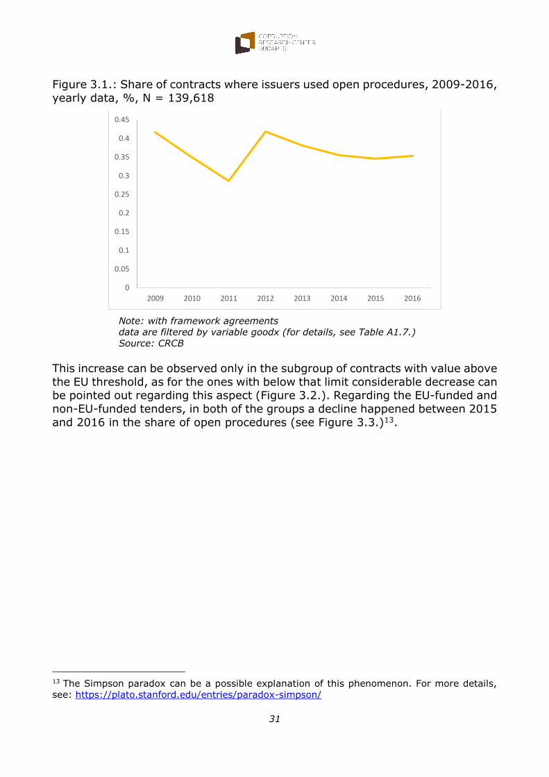
The ratio of open procedures increased less than 1 percentage point, from 34.6% to 35.3% between 2015 and 2016 (see Table 3.1. and Figure 3.1.).
11 Open procedures introduced by the Act CXLIII of 2015 on Public Procurement and discussed
later in this section are not considered to be open in the case of this calculation. 12 Call for tenders is available for every potential bidder, thereby not only the favoured
companies can apply.
30
Table 3.1. Share and number of contracts by the openness of the procurement
procedure, yearly data, 2009-2016, N = 139,618
year Not open Open Total
2009 9,043 6,440 15,483
% 58.41 41.59 100
2010 12,644 6,806 19,450
% 65.01 34.99 100
2011 5,406 2,163 7,569
% 71.42 28.58 100
2012 7,894 5,697 13,591
% 58.08 41.92 100
2013 13,531 8,315 21,846
% 61.94 38.06 100
2014 14,897 8,205 23,102
% 64.48 35.52 100
2015 15,045 7,946 22,991
% 65.44 34.56 100
2016 10,079 5,507 15,586
% 64.67 35.33 100
Total 88,539 51,079 139,618
63.42 36.58 100 Note: with framework agreements
data are filtered by variable goodx (for details, see Table A1.7.)
Source: CRCB
31
Figure 3.1.: Share of contracts where issuers used open procedures, 2009-2016,
yearly data, %, N = 139,618
Note: with framework agreements
data are filtered by variable goodx (for details, see Table A1.7.)
Source: CRCB
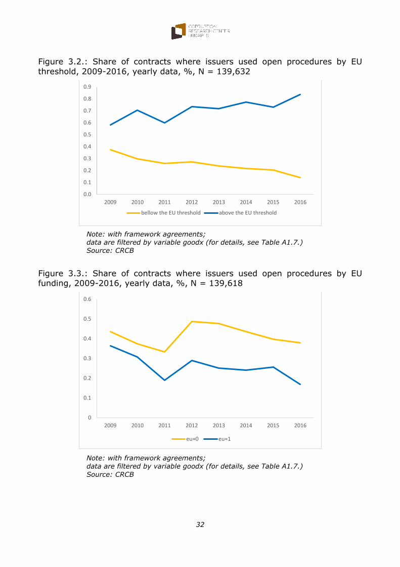
This increase can be observed only in the subgroup of contracts with value above
the EU threshold, as for the ones with below that limit considerable decrease can be pointed out regarding this aspect (Figure 3.2.). Regarding the EU-funded and
non-EU-funded tenders, in both of the groups a decline happened between 2015
and 2016 in the share of open procedures (see Figure 3.3.)13.
13 The Simpson paradox can be a possible explanation of this phenomenon. For more details,
Figure 3.2.: Share of contracts where issuers used open procedures by EU
threshold, 2009-2016, yearly data, %, N = 139,632
Note: with framework agreements;
data are filtered by variable goodx (for details, see Table A1.7.)
Source: CRCB
Figure 3.3.: Share of contracts where issuers used open procedures by EU funding, 2009-2016, yearly data, %, N = 139,618
Note: with framework agreements;
data are filtered by variable goodx (for details, see Table A1.7.)
Source: CRCB
0.0
0.1
0.2
0.3
0.4
0.5
0.6
0.7
0.8
0.9
2009 2010 2011 2012 2013 2014 2015 2016
bellow the EU threshold above the EU threshold
0
0.1
0.2
0.3
0.4
0.5
0.6
2009 2010 2011 2012 2013 2014 2015 2016
eu=0 eu=1
33
We constructed an indicator which gives us information on transparency of
procedures (Transparency Index). We define the Transparency Index (TI) in the following way:
TI = 0, if the tender was issued, without announcement; and
TI = 1 if the tender was issued transparently, i.e. with
announcement.
Firstly, we analyse the evolution of TI over the period in several subgroups of
tenders, then we focus on the evolution of single-bidders and then the composite indicators of corruption risk.
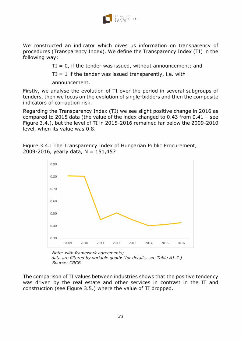
Regarding the Transparency Index (TI) we see slight positive change in 2016 as compared to 2015 data (the value of the index changed to 0.43 from 0.41 – see
Figure 3.4.), but the level of TI in 2015-2016 remained far below the 2009-2010 level, when its value was 0.8.
Figure 3.4.: The Transparency Index of Hungarian Public Procurement,
2009-2016, yearly data, N = 151,457
Note: with framework agreements;
data are filtered by variable goodx (for details, see Table A1.7.)
Source: CRCB
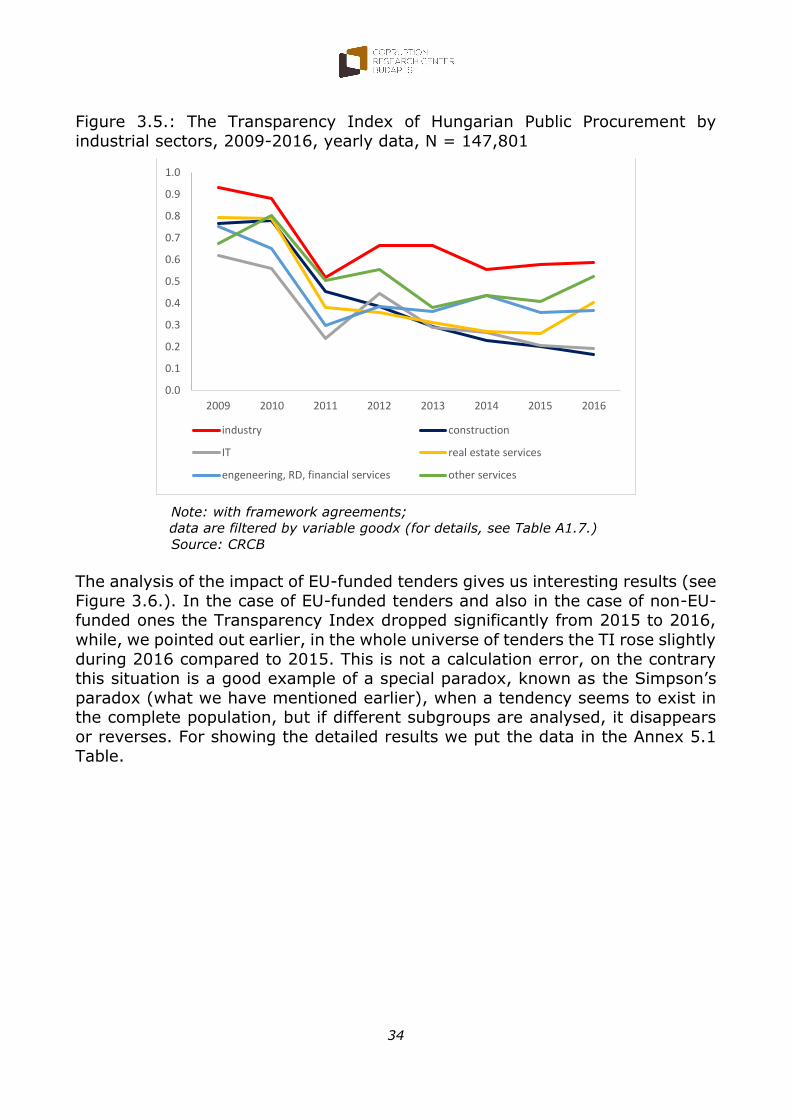
The comparison of TI values between industries shows that the positive tendency was driven by the real estate and other services in contrast in the IT and
construction (see Figure 3.5.) where the value of TI dropped.
0.30
0.40
0.50
0.60
0.70
0.80
0.90
2009 2010 2011 2012 2013 2014 2015 2016
34
Figure 3.5.: The Transparency Index of Hungarian Public Procurement by
industrial sectors, 2009-2016, yearly data, N = 147,801
Note: with framework agreements;
data are filtered by variable goodx (for details, see Table A1.7.)
Source: CRCB
The analysis of the impact of EU-funded tenders gives us interesting results (see
Figure 3.6.). In the case of EU-funded tenders and also in the case of non-EU-funded ones the Transparency Index dropped significantly from 2015 to 2016,
while, we pointed out earlier, in the whole universe of tenders the TI rose slightly
during 2016 compared to 2015. This is not a calculation error, on the contrary this situation is a good example of a special paradox, known as the Simpson’s
paradox (what we have mentioned earlier), when a tendency seems to exist in the complete population, but if different subgroups are analysed, it disappears
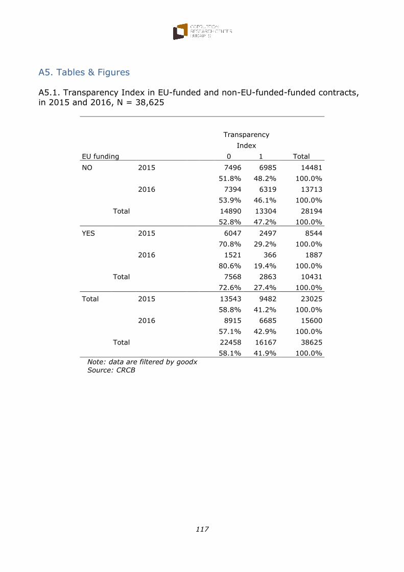
or reverses. For showing the detailed results we put the data in the Annex 5.1 Table.
0.0
0.1
0.2
0.3
0.4
0.5
0.6
0.7
0.8
0.9
1.0
2009 2010 2011 2012 2013 2014 2015 2016
industry construction
IT real estate services
engeneering, RD, financial services other services
35
Figure 3.6.: The Transparency Index of Hungarian Public Procurement in EU-
funded and non-EU-funded tenders, 2009-2016, yearly data, N = 150,942
Note: with framework agreements;
data are filtered by variable goodx (for details, see Table A1.7.)
Source: CRCB
The explanation of these paradoxical results is based on two factors. First, since 2001, the EU-funded tenders have significantly lower TI value in each year than
the non-EU-funded ones, second, the share of the EU-funded tenders dropped
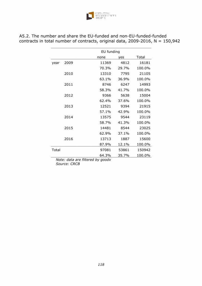
significantly from 2015 to 2016 (from 37% to 12%). Accordingly, the later, because their negligible weight in the total number of contracts much less
reduced the Transparency Index in the overall population than before.
This fall can be corrected if for the purpose of estimation, we assign the same
weight to EU-funded tenders in 2016 as the weight was in the previous year. In this case, we can eliminate the effect of considerable drop of EU-funded project
to the level of Transparency Index.
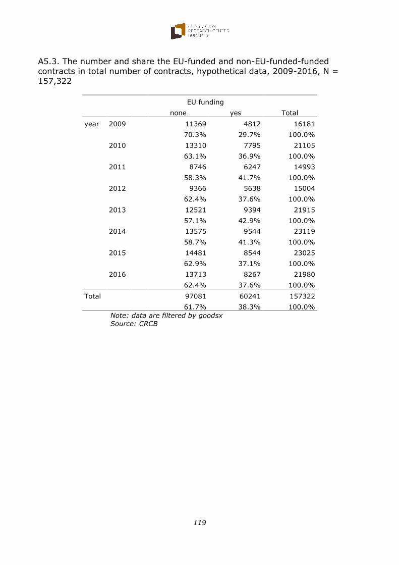
To create a hypothetical dataset and achieve the purpose of the estimation, we
used the following method: we put 6,380 EU-funded contracts from the year of 2015 to the year of 2016 data. Thus, we got a hypothetical dataset with the
same weight of EU-funded project in 2016 as we had in 2015 (see A5.3. Table).
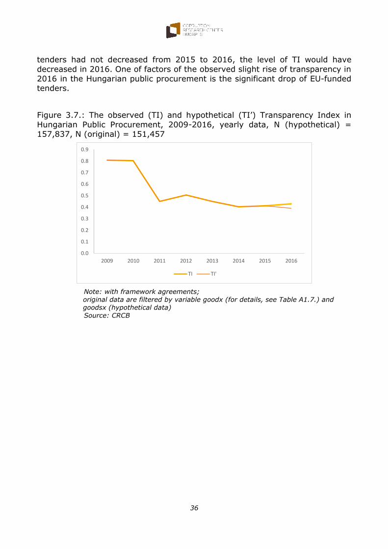
In the original dataset, we can also observe that the value of TI dropped
significantly in the EU-funded projects (from 0.29 to 0.19) between 2015 and 2016. But processing the estimation for the imputed data of 2016 we calculated
0.29 TI value instead of 0.19, so in the hypothetical data of 2016 we used higher
level of TI than we observed for 2016 in the reality. Nonetheless in the supplemented hypothetical dataset we get slightly lower level of TI (0.39) in
2016 compared to 2015 (see Figure 3.7.). This means, if the share of EU-funded
0.0
0.1
0.2
0.3
0.4
0.5
0.6
0.7
0.8
0.9
2009 2010 2011 2012 2013 2014 2015 2016
eu=0 eu=1
36
tenders had not decreased from 2015 to 2016, the level of TI would have
decreased in 2016. One of factors of the observed slight rise of transparency in
2016 in the Hungarian public procurement is the significant drop of EU-funded tenders.
Figure 3.7.: The observed (TI) and hypothetical (TI’) Transparency Index in
Hungarian Public Procurement, 2009-2016, yearly data, N (hypothetical) = 157,837, N (original) = 151,457
Note: with framework agreements;
original data are filtered by variable goodx (for details, see Table A1.7.) and
goodsx (hypothetical data)
Source: CRCB
0.0
0.1
0.2
0.3
0.4
0.5
0.6
0.7
0.8
0.9
2009 2010 2011 2012 2013 2014 2015 2016
TI TI'
37
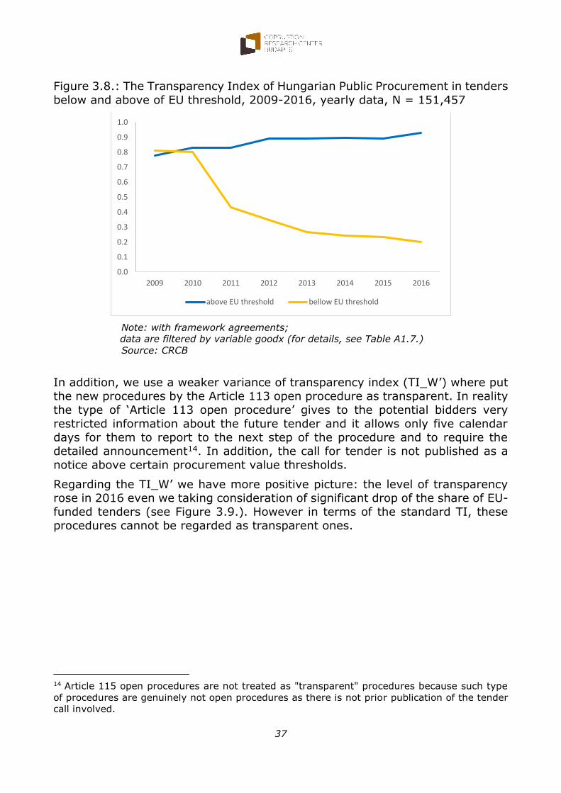
Figure 3.8.: The Transparency Index of Hungarian Public Procurement in tenders
below and above of EU threshold, 2009-2016, yearly data, N = 151,457
Note: with framework agreements;
data are filtered by variable goodx (for details, see Table A1.7.)
Source: CRCB
In addition, we use a weaker variance of transparency index (TI_W’) where put the new procedures by the Article 113 open procedure as transparent. In reality
the type of ‘Article 113 open procedure’ gives to the potential bidders very
restricted information about the future tender and it allows only five calendar days for them to report to the next step of the procedure and to require the
detailed announcement14. In addition, the call for tender is not published as a notice above certain procurement value thresholds.
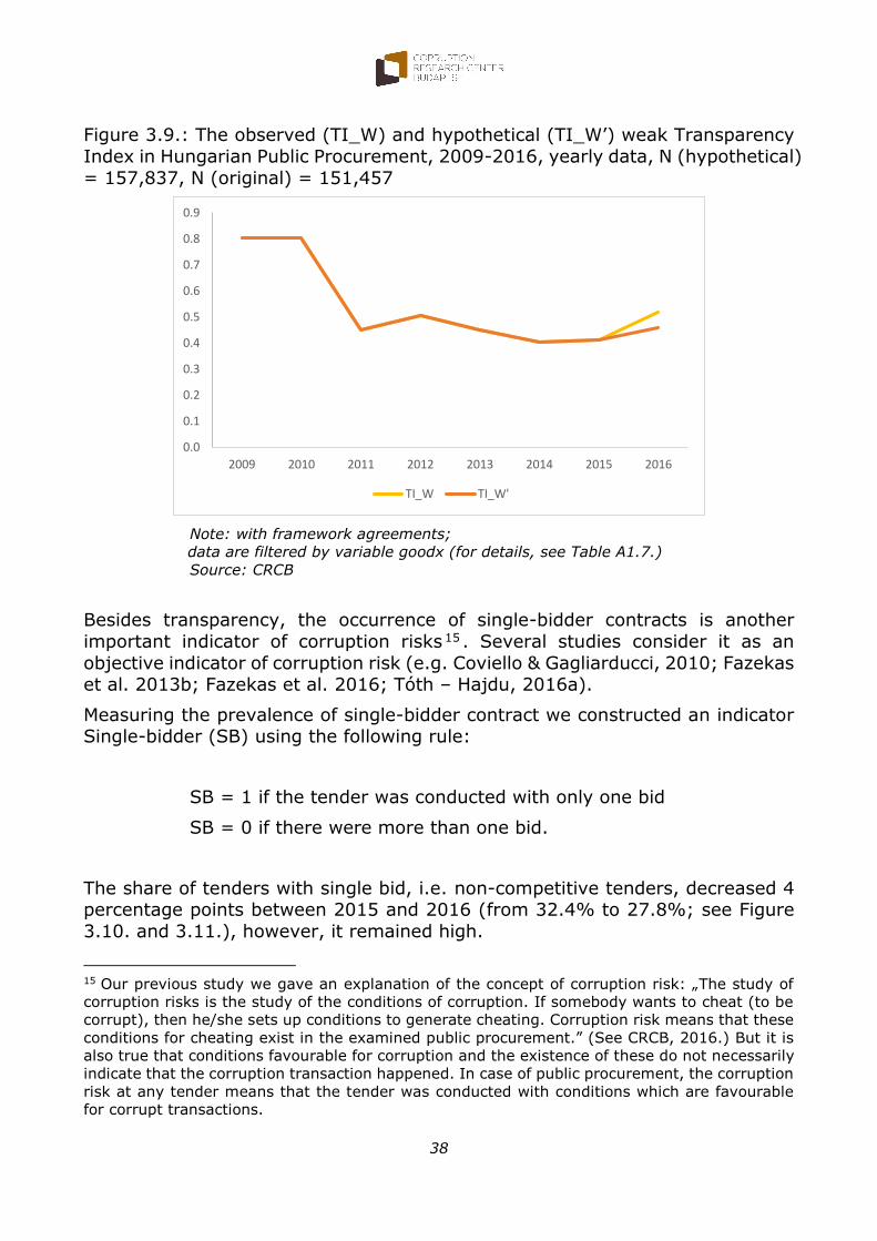
Regarding the TI_W’ we have more positive picture: the level of transparency rose in 2016 even we taking consideration of significant drop of the share of EU-
funded tenders (see Figure 3.9.). However in terms of the standard TI, these procedures cannot be regarded as transparent ones.
14 Article 115 open procedures are not treated as "transparent" procedures because such type
of procedures are genuinely not open procedures as there is not prior publication of the tender
call involved.
0.0
0.1
0.2
0.3
0.4
0.5
0.6
0.7
0.8
0.9
1.0
2009 2010 2011 2012 2013 2014 2015 2016
above EU threshold bellow EU threshold
38
Figure 3.9.: The observed (TI_W) and hypothetical (TI_W’) weak Transparency
Index in Hungarian Public Procurement, 2009-2016, yearly data, N (hypothetical)
= 157,837, N (original) = 151,457
Note: with framework agreements;
data are filtered by variable goodx (for details, see Table A1.7.)
Source: CRCB
Besides transparency, the occurrence of single-bidder contracts is another
important indicator of corruption risks 15 . Several studies consider it as an
objective indicator of corruption risk (e.g. Coviello & Gagliarducci, 2010; Fazekas et al. 2013b; Fazekas et al. 2016; Tóth – Hajdu, 2016a).
Measuring the prevalence of single-bidder contract we constructed an indicator Single-bidder (SB) using the following rule:
SB = 1 if the tender was conducted with only one bid
SB = 0 if there were more than one bid.
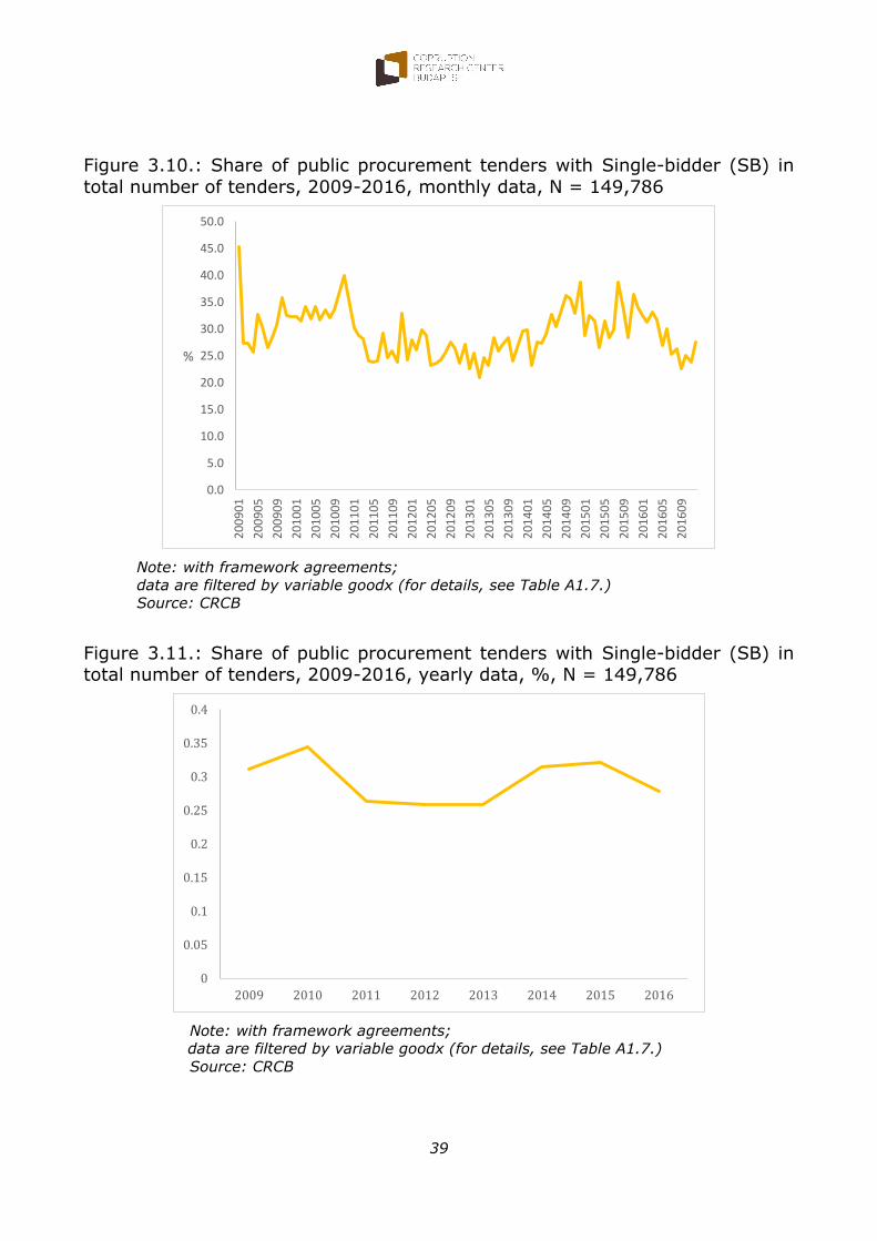
The share of tenders with single bid, i.e. non-competitive tenders, decreased 4 percentage points between 2015 and 2016 (from 32.4% to 27.8%; see Figure
3.10. and 3.11.), however, it remained high.
15 Our previous study we gave an explanation of the concept of corruption risk: „The study of
corruption risks is the study of the conditions of corruption. If somebody wants to cheat (to be
corrupt), then he/she sets up conditions to generate cheating. Corruption risk means that these
conditions for cheating exist in the examined public procurement.” (See CRCB, 2016.) But it is
also true that conditions favourable for corruption and the existence of these do not necessarily
indicate that the corruption transaction happened. In case of public procurement, the corruption
risk at any tender means that the tender was conducted with conditions which are favourable
for corrupt transactions.
0.0
0.1
0.2
0.3
0.4
0.5
0.6
0.7
0.8
0.9
2009 2010 2011 2012 2013 2014 2015 2016
TI_W TI_W'
39
Figure 3.10.: Share of public procurement tenders with Single-bidder (SB) in
total number of tenders, 2009-2016, monthly data, N = 149,786
Note: with framework agreements;
data are filtered by variable goodx (for details, see Table A1.7.)
Source: CRCB
Figure 3.11.: Share of public procurement tenders with Single-bidder (SB) in total number of tenders, 2009-2016, yearly data, %, N = 149,786
Note: with framework agreements;
data are filtered by variable goodx (for details, see Table A1.7.)
Source: CRCB
0.0
5.0
10.0
15.0
20.0
25.0
30.0
35.0
40.0
45.0
50.02
00
90
1
20
09
05
20
09
09
20
10
01
20
10
05
20
10
09
20
11
01
20
11
05
20
11
09
20
12
01
20
12
05
20
12
09
20
13
01
20
13
05
20
13
09
20
14
01
20
14
05
20
14
09
20
15
01
20
15
05
20
15
09
20
16
01
20
16
05
20
16
09
%
0
0.05
0.1
0.15
0.2
0.25
0.3
0.35
0.4
2009 2010 2011 2012 2013 2014 2015 2016
40
Regarding the monthly average, during the I-III. quarters of 2016 was
characterised by falling tendency, by in the IV. quarters the corruption risks
measured by the share of single-bidder started to increase (see Figure 3.10.).
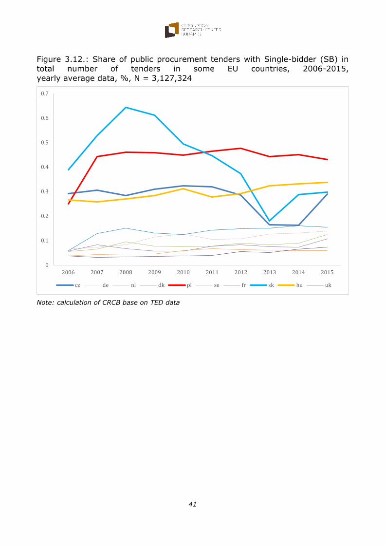
In international comparison on the basis of the TED database, the share of
tenders with only a single-bidder is notably high in Hungary, varying between 25% and 33% in 2006–2015 (see Figure 3.12.). During the same period, the
share of non-competitive tenders did not exceed 12% in the old EU member states (for instance, Denmark, France, the Netherlands, Germany and Sweden)
16. This is a clear sign that Hungarian public procurement tenders are strongly affected by corruption risks.
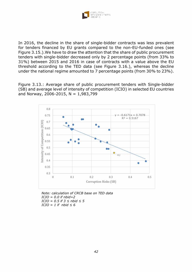
However, it has to be kept in mind, that the dissimilarities in the level of development of market economies and therefore in the share and number of
large firms may influence the SB indicator. Taking consideration the intensity of competition we have similar results: the Hungarian public tenders have in
average one of the lowest intensity of competition compared to the other European countries (see 3.13.)
16 A possible interpretation for the relatively high ratio of contracts with single-bidder in Hungary
in EU comparison can be related to the differences in the national socio-economic environments.
More specifically, the limited number of potent companies operating in certain sectors can affect
this indicator. However, the investigations of the CRCB prove that this concern has only a
marginal effect on the index; for example it is significantly correlated to the corruption
perceptions (see: http://bitly.com/1Yc7zQL ). In addition, the TED data reveals that even
smaller countries than Hungary from the post-socialist region can perform better from this point
of view, like Latvia and Slovenia (see: http://bit.ly/2ywlZXJ).
Figure 3.12.: Share of public procurement tenders with Single-bidder (SB) in
total number of tenders in some EU countries, 2006-2015,
yearly average data, %, N = 3,127,324
Note: calculation of CRCB base on TED data
0
0.1
0.2
0.3
0.4
0.5
0.6
0.7
2006 2007 2008 2009 2010 2011 2012 2013 2014 2015
cz de nl dk pl se fr sk hu uk
42
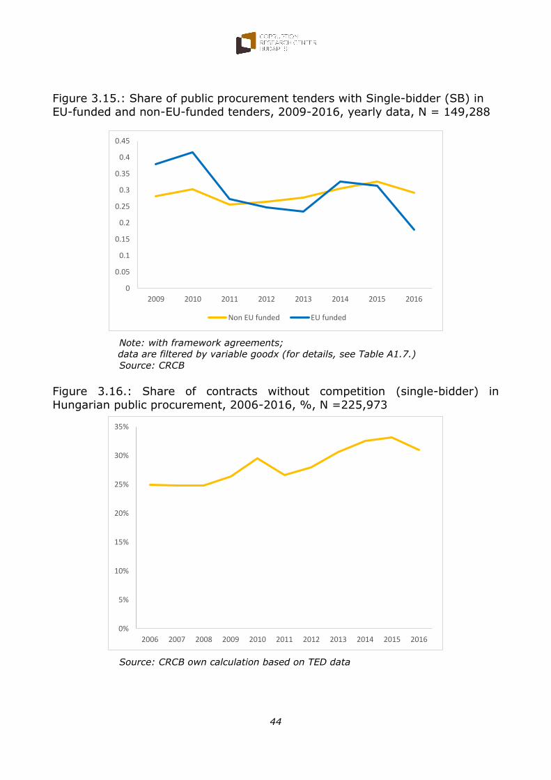
In 2016, the decline in the share of single-bidder contracts was less prevalent for tenders financed by EU grants compared to the non-EU-funded ones (see
Figure 3.15.).We have to draw the attention that the share of public procurement tenders with single-bidder decreased only by 2 percentage points (from 33% to
31%) between 2015 and 2016 in case of contracts with a value above the EU threshold according to the TED data (see Figure 3.16.), whereas the decline
under the national regime amounted to 7 percentage points (from 30% to 23%).
Figure 3.13.: Average share of public procurement tenders with Single-bidder (SB) and average level of intensity of competition (ICIO) in selected EU countries
and Norway, 2006-2015, N = 1,983,799
Note: calculation of CRCB base on TED data
ICIO = 0.0 if nbid=2
ICIO = 0.5 if 3 ≤ nbid ≤ 5
ICIO = 1 if nbid ≤ 6
y = -0.6171x + 0.7078R² = 0.5167
0.3
0.35
0.4
0.45
0.5
0.55
0.6
0.65
0.7
0.75
0.8
0 0.1 0.2 0.3 0.4 0.5
Inte
nsi
ty o
f C
om
pet
itio
n (
ICIO
)
Corruption Risks (SB)
HU
43
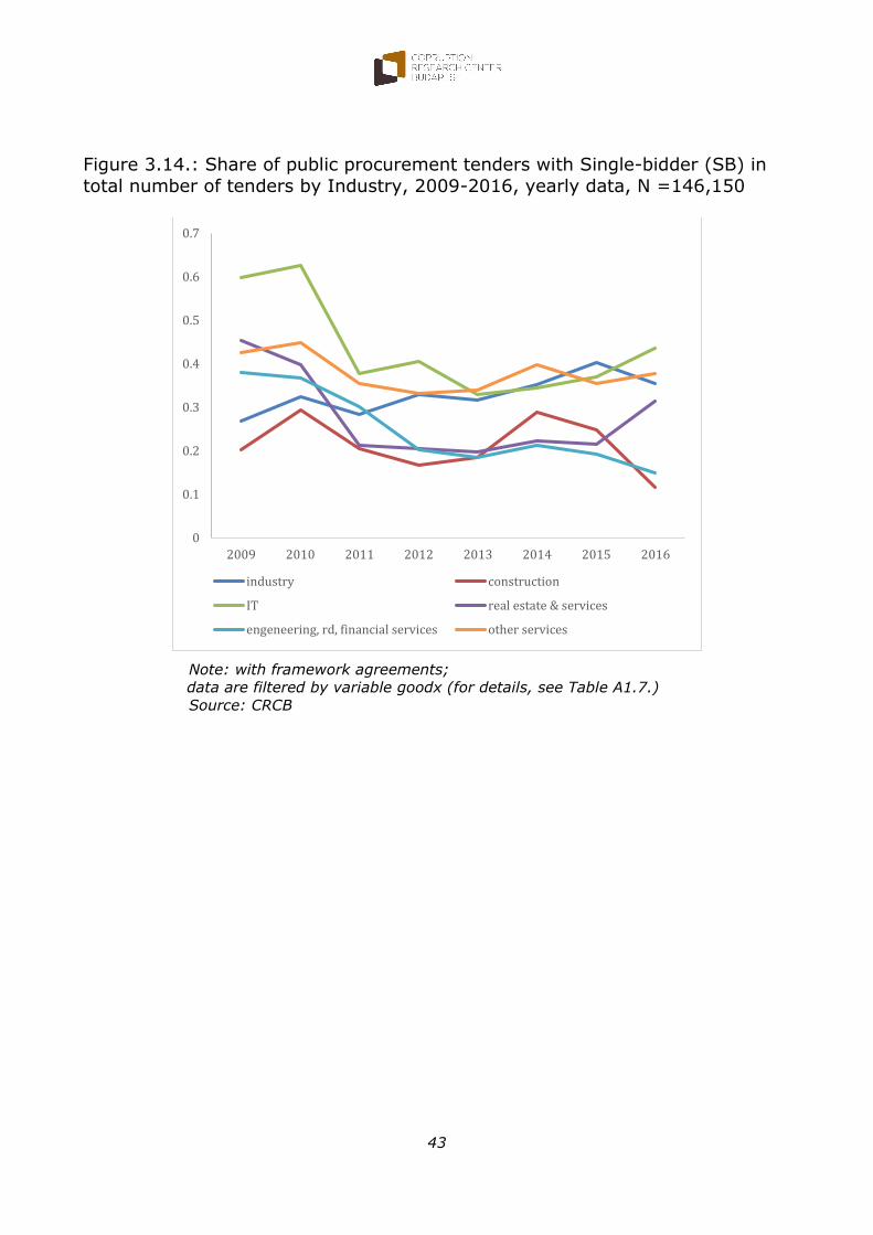
Figure 3.14.: Share of public procurement tenders with Single-bidder (SB) in
total number of tenders by Industry, 2009-2016, yearly data, N =146,150
Note: with framework agreements;
data are filtered by variable goodx (for details, see Table A1.7.)
Source: CRCB
0
0.1
0.2
0.3
0.4
0.5
0.6
0.7
2009 2010 2011 2012 2013 2014 2015 2016
industry construction
IT real estate & services
engeneering, rd, financial services other services
44
Figure 3.15.: Share of public procurement tenders with Single-bidder (SB) in
EU-funded and non-EU-funded tenders, 2009-2016, yearly data, N = 149,288
Note: with framework agreements;
data are filtered by variable goodx (for details, see Table A1.7.)
Source: CRCB
Figure 3.16.: Share of contracts without competition (single-bidder) in
Hungarian public procurement, 2006-2016, %, N =225,973
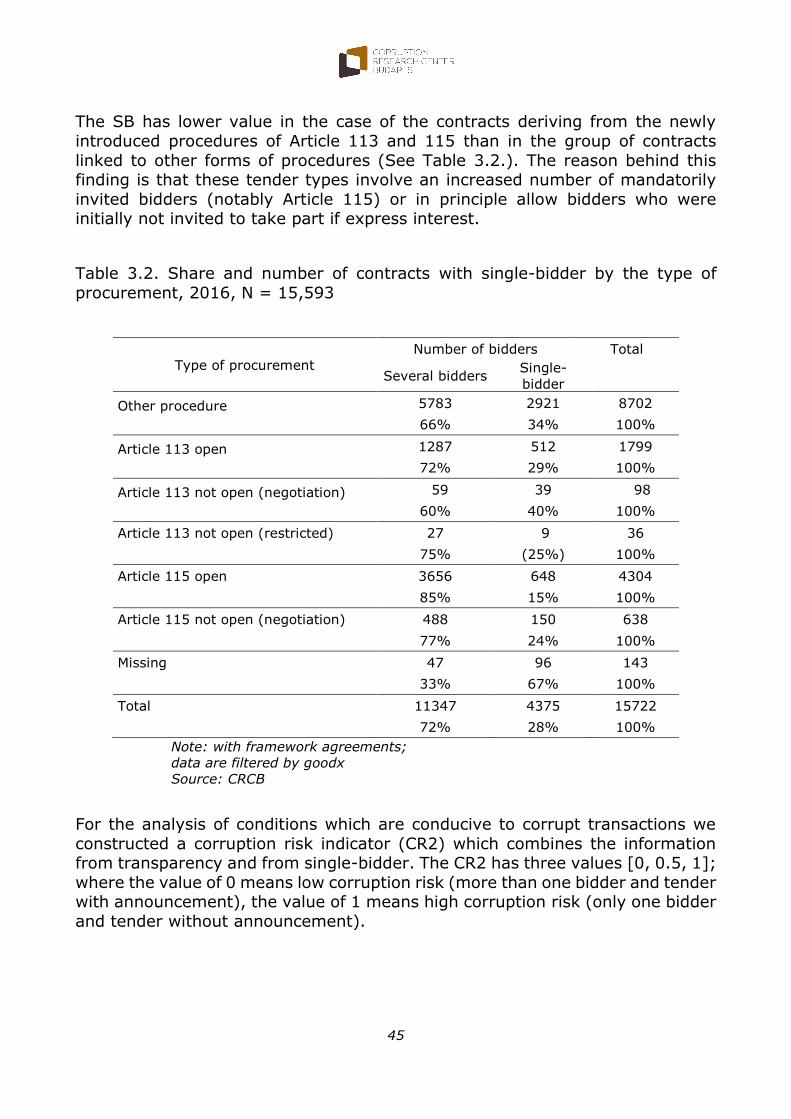
The SB has lower value in the case of the contracts deriving from the newly
introduced procedures of Article 113 and 115 than in the group of contracts
linked to other forms of procedures (See Table 3.2.). The reason behind this finding is that these tender types involve an increased number of mandatorily
invited bidders (notably Article 115) or in principle allow bidders who were initially not invited to take part if express interest.
Table 3.2. Share and number of contracts with single-bidder by the type of
procurement, 2016, N = 15,593
Type of procurement
Number of bidders Total
Several bidders Single-
bidder
Other procedure
5783 2921 8702
66% 34% 100%
Article 113 open
1287 512 1799
72% 29% 100%
Article 113 not open (negotiation)
59 39 98
60% 40% 100%
Article 113 not open (restricted) 27 9 36
75% (25%) 100%
Article 115 open 3656 648 4304
85% 15% 100%
Article 115 not open (negotiation) 488 150 638
77% 24% 100%
Missing 47 96 143
33% 67% 100%
Total 11347 4375 15722
72% 28% 100%
Note: with framework agreements;
data are filtered by goodx Source: CRCB
For the analysis of conditions which are conducive to corrupt transactions we
constructed a corruption risk indicator (CR2) which combines the information from transparency and from single-bidder. The CR2 has three values [0, 0.5, 1];
where the value of 0 means low corruption risk (more than one bidder and tender with announcement), the value of 1 means high corruption risk (only one bidder
and tender without announcement).
46
The formula of CR2 is the following:
𝐶𝑅2 =(1−𝑇𝐼)+𝑆𝐵
2 (2)
We have also used an augmented corruption risk indicator. The pricing behaviour of winner companies differs significantly in corrupt and non-corrupt cases.
According to the fraud analytics the actors (in our case the winner companies) tend to use rounded data in cases when fraud happened, and they use rounded
prices less frequently in normal cases. One of the methods to detect the fraud is to analyse the occurrence of rounded data (Nigrini, 2012; Spann, 2013; Miller,
2015). In terms of corruption, rounded prices could be regarded as a further sign of low competition and higher level of corruption risks. Taking into account
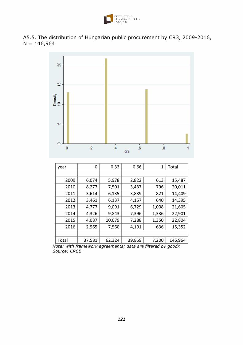
this consideration, we augmented the CR2 indicator with information on rounding by at least 10,000 and constructed a new corruption risk indicator (CR3)
which contains information on transparency, single-bidder and on rounded
contract prices17 as well. The CR3 has four values: 0, 0.33, 0.66, 1. The value of 0 means low corruption risk (more than one bidder, tender with
announcement, and not rounded price), the value of 1 means high corruption risk (only one bidder, tender without announcement and rounded price).
We constructed the CR3 using the following formula:
if CR2=0 & ROUND4 =0 then CR3 =0
if CR2=0 & ROUND4 =1 then CR3=0.33 if CR2=0.5 & ROUND4 =0 then CR3=0.33
if CR2=0.5 & ROUND4 =1 then CR3=0.66 if CR2=1 & ROUND4 =0 then CR3=0.66
if CR2=1 & ROUND4 =1 then CR3=1
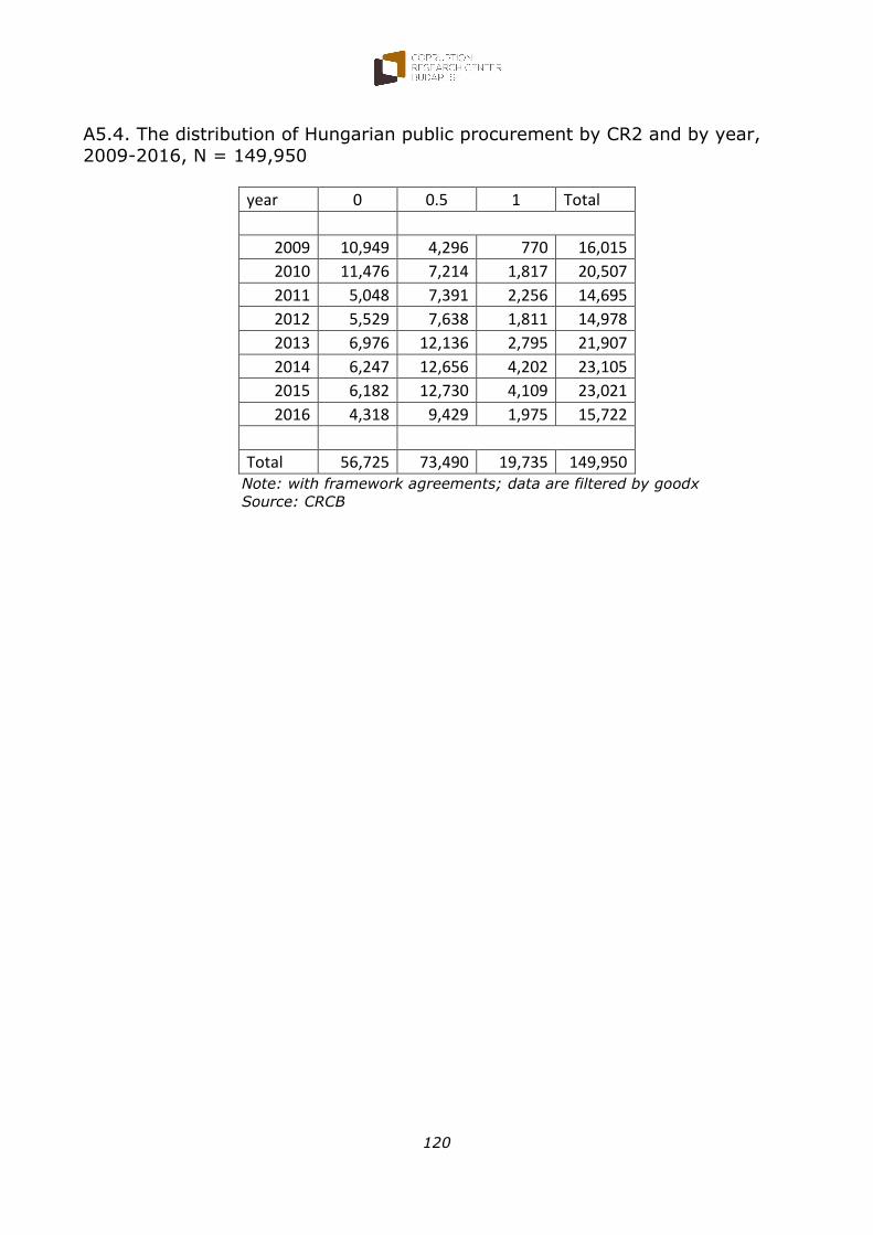
The distribution of Hungarian public tenders by CR3 see Annex 5.5. We
summarise here the most important observations on the evolution of corruption indicators over the period:
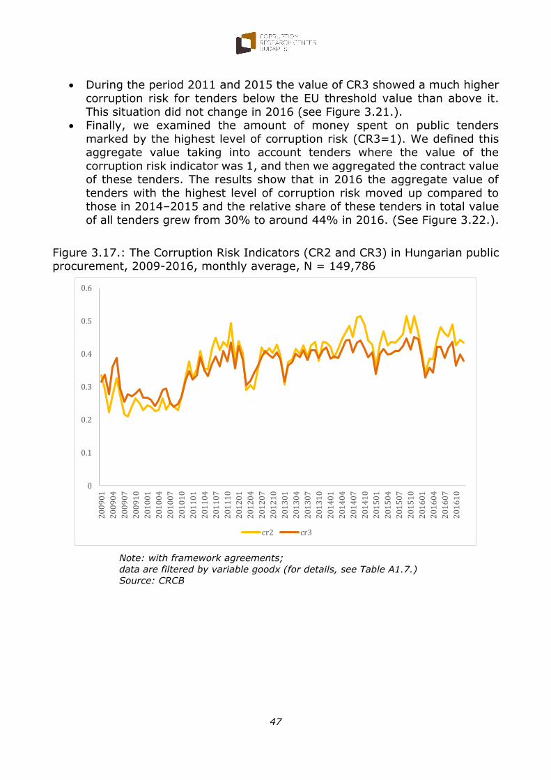
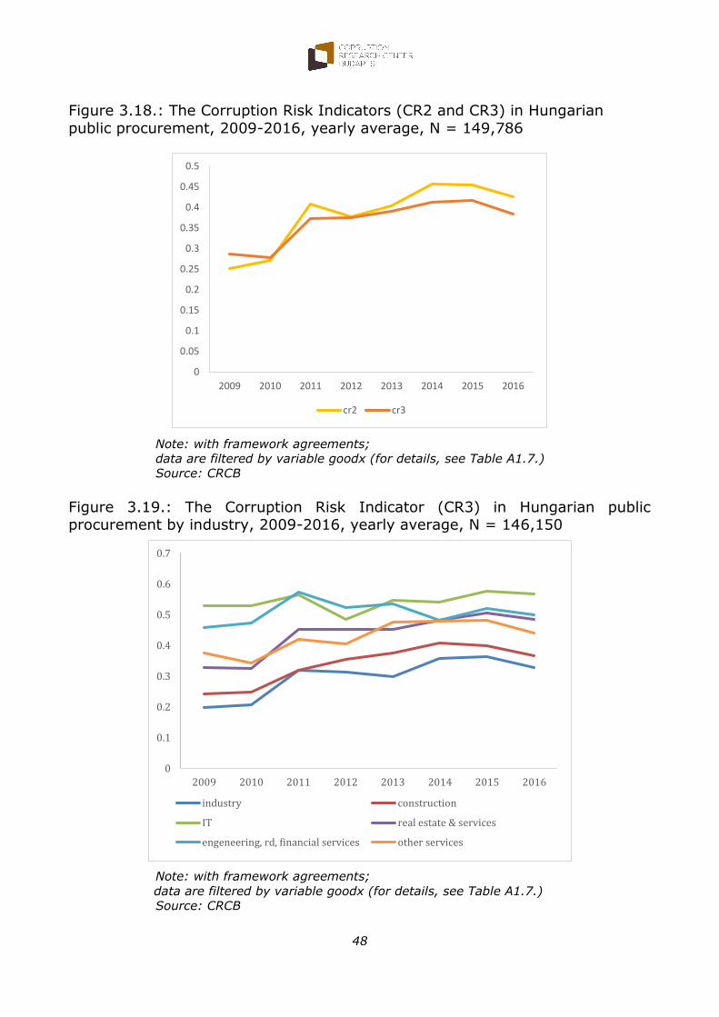
While showing an increasing trend between 2009 and 2015, the average
values of composite corruption risk indicators (CR2 and CR3) fell slightly in 2016 but remained at a relatively high level. The CR2 decreased from
0.46 point to 0.43 point, and the CR3 decreased from 0.52 point to 0.5 point between 2015 and 2016 (see Figure 3.17. and 3.18.).
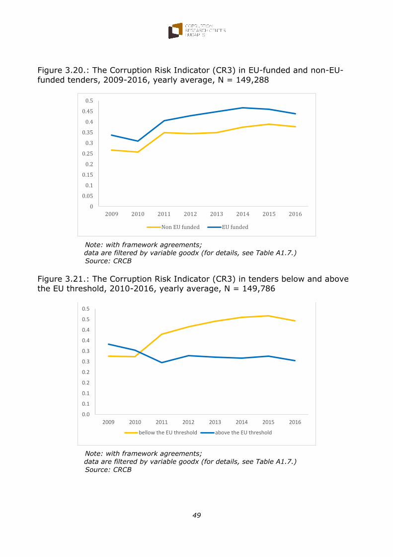
The CR3 decreased in all industries except IT sector (see Figure 3.19.) The CR3 was higher for EU-funded tenders than non-EU-funded ones
between 2010 and 2016 (see Figure 3.20.).
17 On rounded contract prices see the section 5.1.
47
During the period 2011 and 2015 the value of CR3 showed a much higher
corruption risk for tenders below the EU threshold value than above it.
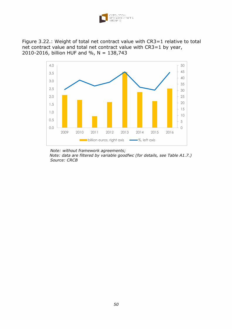
This situation did not change in 2016 (see Figure 3.21.). Finally, we examined the amount of money spent on public tenders
marked by the highest level of corruption risk (CR3=1). We defined this aggregate value taking into account tenders where the value of the
corruption risk indicator was 1, and then we aggregated the contract value of these tenders. The results show that in 2016 the aggregate value of
tenders with the highest level of corruption risk moved up compared to those in 2014–2015 and the relative share of these tenders in total value
of all tenders grew from 30% to around 44% in 2016. (See Figure 3.22.).
Figure 3.17.: The Corruption Risk Indicators (CR2 and CR3) in Hungarian public procurement, 2009-2016, monthly average, N = 149,786
Note: with framework agreements;
data are filtered by variable goodx (for details, see Table A1.7.)
Source: CRCB
0
0.1
0.2
0.3
0.4
0.5
0.6
20
09
01
20
09
04
20
09
07
20
09
10
20
10
01
20
10
04
20
10
07
20
10
10
20
11
01
20
11
04
20
11
07
20
11
10
20
12
01
20
12
04
20
12
07
20
12
10
20
13
01
20
13
04
20
13
07
20
13
10
20
14
01
20
14
04
20
14
07
20
14
10
20
15
01
20
15
04
20
15
07
20
15
10
20
16
01
20
16
04
20
16
07
20
16
10
cr2 cr3
48
Figure 3.18.: The Corruption Risk Indicators (CR2 and CR3) in Hungarian
public procurement, 2009-2016, yearly average, N = 149,786
Note: with framework agreements;
data are filtered by variable goodx (for details, see Table A1.7.)
Source: CRCB
Figure 3.19.: The Corruption Risk Indicator (CR3) in Hungarian public procurement by industry, 2009-2016, yearly average, N = 146,150
Note: with framework agreements;
data are filtered by variable goodx (for details, see Table A1.7.)
Source: CRCB
0
0.05
0.1
0.15
0.2
0.25
0.3
0.35
0.4
0.45
0.5
2009 2010 2011 2012 2013 2014 2015 2016
cr2 cr3
0
0.1
0.2
0.3
0.4
0.5
0.6
0.7
2009 2010 2011 2012 2013 2014 2015 2016
industry construction
IT real estate & services
engeneering, rd, financial services other services
49
Figure 3.20.: The Corruption Risk Indicator (CR3) in EU-funded and non-EU-
funded tenders, 2009-2016, yearly average, N = 149,288
Note: with framework agreements;
data are filtered by variable goodx (for details, see Table A1.7.)
Source: CRCB
Figure 3.21.: The Corruption Risk Indicator (CR3) in tenders below and above the EU threshold, 2010-2016, yearly average, N = 149,786
Note: with framework agreements;
data are filtered by variable goodx (for details, see Table A1.7.)
Source: CRCB
0
0.05
0.1
0.15
0.2
0.25
0.3
0.35
0.4
0.45
0.5
2009 2010 2011 2012 2013 2014 2015 2016
Non EU funded EU funded
0.0
0.1
0.1
0.2
0.2
0.3
0.3
0.4
0.4
0.5
0.5
2009 2010 2011 2012 2013 2014 2015 2016
bellow the EU threshold above the EU threshold
50
Figure 3.22.: Weight of total net contract value with CR3=1 relative to total
net contract value and total net contract value with CR3=1 by year, 2010-2016, billion HUF and %, N = 138,743
Note: without framework agreements;
Note: data are filtered by variable goodfwc (for details, see Table A1.7.)
Source: CRCB
0
5
10
15
20
25
30
35
40
45
50
0.0
0.5
1.0
1.5
2.0
2.5
3.0
3.5
4.0
2009 2010 2011 2012 2013 2014 2015 2016
billion euros, right axis %, left axis
51
4. Price distortion
In this section we focus on the analysis of net contract prices to detect price
distortion or overpricing. The concept of the price distortion/overpricing is also related to corruption (see Table 1). We consider the former as an outcome of a
corrupt situation. In the case of a corrupt tender, the contract price includes the economic rent generated by corruption in addition to the market price. As a
consequence, price setting within corrupt tenders must be fundamentally different from that of tenders involving competition.
As a result, the prices of corrupt tenders contain additional information that is not included in the prices of tenders with competition. Compared to prices of
tenders with competition, the prices of corrupt tenders have to show different characteristics. Besides our earlier indicators of corruption risk, as SB, or CR2,
it is also important to pay attention to information in contract price, and to analyse them. While SB and CR2 purely focus on the (pre)conditions of
corruption, the analysis of contract prices already takes into account its
consequences, or outcomes. Indeed, because of corruption, contract prices of corrupt tenders could be distorted as compared to prices of tenders with high
level of competition.
For the reasons explained above we interpret the price distortion as a sign of
non-zero level of corruption risk. We use three methods to detect this phenomenon: we analyse (i) the rounded data in contract prices; (ii) the
observed distribution of first digits of net contract price against distribution of first digits predicted by the Benford’s law; and, finally (iii) the drop in contract
prices compared to the estimated value of tenders (i.e. the price estimated by the issuer and published in the call for tenders).
4.1. Rounded data in contract prices
Rounded contract prices can be regarded as an indicator of existence of price distortion. The analysis of rounded data is one of tool the tools of fraud analytics
to detect irregularities in prices (Miller, 2015, Nigrini, 2012 and Spann, 2013). We constructed three indicators for this analysis: ROUND4, ROUND5 and
ROUNDR2. We defined them in the following way:
ROUND4 = 1, if the contract price is divisible by at least 104
without remainder (rounded at thousands)
ROUND4 = 0, if the contract price is not divisible by 104 without remainder
ROUND5 = 1, if the contract price is divisible by at least 105
without remainder (rounded at thousands)
ROUND5 = 0, if the contract price is not divisible by 105
52
without remainder
Due to the fact that the weight of the possible rounding depends also on the size
of the numbers we calculated a relative index, the round ratio (ROUNDR) using the following formula:
𝑅𝑂𝑈𝑁𝐷𝑅 = 𝑅𝑜𝑏𝑠
𝑅𝑚𝑎𝑥 (3)
Where Robs is the number of maximal level rounding of the given contract price. For instance, if the contract price is 24,500 HUF the value of Robs is
2, and if it is 456,000,000 HUF the value of Robs 6. The Rmax means the maximum weight of rounding at certain size of numbers. For instance, for
the contract prices between 10,000 and 99,999 HUF the value of Rmax is 4 and prices between 100,000,000 and 999,999,999 HUF the Rmax is 8.
In the next step we recoded the value of ROUNDR into a new variable (ROUNDR2) which has 4 categories [0.25, 0.5, 0.75 and 1] where the highest value means
the highest weight of rounding at the given contract price.
We interpret the value the ROUNDR2 as a proxy of the strength of non-competitive (or non-cost based) pricing: lower level of ROUNDR2 means higher
level of competition and lower level of corruption risk and higher level of ROUNDR2 means a reverse tendency.
The indicators of rounded prices (ROUND4 and ROUND5) show a decreasing
trend in price distortion in the last three years from 35.8% to 29.0%, however, the ROUND4 is still close 0.30, it means that around 30% of the contract prices
were rounded by 104 in the Hungarian public procurement (see Figure 4.1.1.). This decline can be considered as an important feature of public tenders because
the change in the price setting behaviour of winners is the result of a
spontaneous agent-level based process, which, for instance, is not driven by the requirements by public procurement law or by regulators. (In the case of the
number of bidders, we can expect such institutional effect when the public procurement law in certain procedures clearly specifies the minimum number of
bidders.)
The decreasing trend in the share of rounded prices is not present in every segment of tenders, and it is largely driven by the construction sector. In the
sector of engineering, RD, financial and other services and also in the industry, the share of rounded prices stagnated or showed a slight increase between 2012
and 2016 (see Figure 4.1.2.). Surprisingly in the construction sector the contract prices are significantly less frequently rounded than in other industries (only
29%-12% of the cases). We assume that this fact is related to the widespread
53
use of the cost estimation manuals18 by the bidders from the construction sector.
And additionally, in the construction sector the actors regularly use the method of supplementary works to raise the initial contract prices and thus, to get the
rent generated by corruption. Unfortunately, due to the missing data, however we do not have accurate information on their frequency and extent. It can be
seen that if we take the original contract prices into consideration, the cost based pricing could be more often found in construction than in other industrial sectors19.
As it was expected, the occurrence of rounded data in contract prices has positive statistical relationship with the corruption risk: the winners of tenders
with high level of corruption risk use the rounded data in their prices more often than in the case of tenders with low level of corruption risk (See Figure 4.1.3.
and A5.6 and A5.7). Where the tender was performed with high corruption risk, a higher share of contract price was rounded by at least 104 (35.4%) than in the
case of those with low corruption risk (26.8%). The analysis of the weight of rounded data (ROUNDR) shows us the same picture (See Figure 4.1.4.).
Finally, we analysed the price distortion measured by rounding (ROUND4,
ROUND5) and the EU funding (See Figure 4.1.5.). The results point out that the EU-funded tenders have higher share of rounded data than the non-EU-funded
ones. When we control for the contract value, sector and date of the tenders the results are contradictory. In case of ROUND4 there is strong positive and in case
of ROUND5 there is less powerful negative correlation between the rounded price
and the EU funding (see A5.6 and A5.7).
Given the fact that the corruption risks are higher and the intensity of competition is lower amongst the EU-funded projects than amongst the non-EU-
funded ones, this new empirical evidence points out the hypothesis that the EU support can incur contradictory effects on price distortion. It cannot be
demonstrated that the EU funding would clearly reduce the level of price distortion. (For the detailed analysis of effects of EU funds see the section 5.3.)
18 See for instance: http://bit.ly/2k4MHA2 . The manual is published and refreshed yearly. 19 In the construction sector corruption risks maybe related to a lesser degree to overpricing (in
case of original contract price) rather than to enforcing supplementary work or bid rigging.
Figure 4.1.1.: Evolution of value of ROUND4, ROUND5 and ROUNDR2 over the
period of 2009-2016, yearly average N (ROUND4 and ROUND5) = 138,743,
N (ROUNDR2) = 93,004
Note: without framework agreements;
data are filtered by goodfwc and the cases are excluded where currency is other than HUF
Source: CRCB
Figure 4.1.2.: The evolution of ROUND4 by industrial sectors, yearly average,
2010-2016, N = 135,327
Note: without framework agreements;
data are filtered by goodfwc and the cases are excluded where currency is other than HUF
Source: CRCB
0
0.1
0.2
0.3
0.4
0.5
0.6
0.7
0.8
2009 2010 2011 2012 2013 2014 2015 2016
round4 round5 roundr2
0
0.1
0.2
0.3
0.4
0.5
0.6
0.7
0.8
0.9
2009 2010 2011 2012 2013 2014 2015 2016
industry construction
IT real estate & services
engeneering, rd, financial services other services
55
Figure 4.1.3.: The share of rounded data in contract price (ROUND4 and
ROUND5) over the period by tenders with low and high level of corruption risk
(CR2), yearly average, 2009-2016, N = 68,810
Note: without framework agreements;
data are filtered by goodfwc and the cases are excluded where currency is other than HUF
Source: CRCB
Figure 4.1.4.: Weight of rounded data (ROUNDR2) in contract prices in tenders with low and high level of corruption risk (CR2), 2010-2016, yearly average,
2010-2016, N = 45,032
Note: without framework agreements;
data are filtered by goodfwc and the cases are excluded where currency is other than HUF
Using the second method, we analyse the price distortion by the distribution of
the first digit in the contract prices based on Benford’s law20 or Newcomb-Benford-s law21.
According to Benford's law (also known as the First-Digit Phenomenon) in a non-artificially generated set of numbers (in any numeral system) the first digits in
each, local values are distributed neither arbitrarily nor uniformly; the distribution instead follows the distribution set by Benford’s law. A set of
numbers is said to satisfy Benford's Law if the leading digit d (in 10 digit system, d ∈ {1, ..., 9}) occurs with probability:
The distribution of first digits in the decimal system (1,..,9) according to
Benford’s law is in Table 4.2.1.
Table 4.2.1. The distribution of first digit according to the Benford’s law in the decimal system
First digits log(d) log(d+1) P(d) = log(d+1) - log(d) cum [P(d)]
1 0.000 0.301 0.301 0.301
2 0.301 0.477 0.176 0.477
3 0.477 0.602 0.125 0.602
4 0.602 0.699 0.097 0.699
5 0.699 0.778 0.079 0.778
6 0.778 0.845 0.067 0.845
7 0.845 0.903 0.058 0.903
8 0.903 0.954 0.051 0.954
9 0.954 1.000 0.046 1.000
The economist Hal Varian first suggested in 1972 that Benford’s law could be used to detect possible fraud in socio-economic data, and that it the performance
of forecasting models could be evaluated (Varian, 1972). Mark Nigrini pointed out 25 years later that Benford's law is useful in forensic accounting and auditing
as a tool to detect fraud and collusion (Nigrini, 1996). Ever since, Benford’s law has been common and it is a widely used method in several areas of social
research for fraud detection Drake & Nigrini, 2000; Durtschi et al. 2004; Spann,
20 In the description of the concept of this method for the detection of price distortion we are
using partially our earlier work. See CRCB, 2016. 21 See https://en.wikipedia.org/wiki/Benford%27s_law
Based on Bendford's law we examined whether the contract price differs
significantly from the hypothetical distribution by the intensity of competition and the presence of corruption risks. We examine these relationships by
comparing the observed first digit’s distribution to theoretical (Benford’s) distribution of contact prices of tenders in several analysed groups of tenders in
the Hungarian public procurement.
The deviation from the distribution predicted by the Benford’s law can be
generated by three factors:
a) the price-setting behaviour of the issuer: the issuer sets the estimated
value of the project by using non-market price methods but by considering how much money is accessible for the project;
b) the price setting behaviour of the winner: during the process to set the bid, the future winner already includes a corruption rent into the offer’s
price.
c) administrative factors or regulation: the laws or resolutions concerning
public procurement arbitrary set thresholds for certain sectors and/or
procedure types;
Of the above three factors the first (a) and the second (b) ones can be explained
more easily. In the case of a) the issuer obviously does not act according to the initial objective of public procurement (i.e. to buy goods or services at market
prices). That is, the public money is not treated by the issuer with the required manner: it does not conduct a market research before the call for tenders, it
does not ensure that the products / services they want to buy at what price can be purchased on the market. In this case, one type of corruption is realised, the
embezzlement or misappropriation of public funds (Lambsdorff, 2007). All of this results in the fact that the contract prices of purchased goods or services deviate
from their expected or normal values (i.e. market prices) and those are rather determined by political / administrative factors (i.e. the political importance of
the project; the bargaining power of the issuer in the negotiations for public resources, etc.). This situation results in obvious distorted prices compared to
market prices and it can be detected by using the Benford’s law.
In the second case (b) the price setting behaviour of future winner is influenced by several factors. First, to what extent the future winner would be able to
establish a corrupt situation before the start of the procurement procedure, and how high the corruption risk is associated with this particular procedure. And,
what the future winner’s expectation or knowledge is on the intensity of competition during this tender or how much he/she knows about the other
competitors' bids.
If there is a high risk of corruption, the rate of the rent due to corruption may
be higher if it is small, then it is lower. If the winner expected a low intensity of competition or ex-ante colluded with the other competitors on the price, the
59
winner would be able to add a rent to his bid price. As a result, the winner’s price
will differ obviously from the market price.
The third case (c) has effects only indirectly. In theory, the thresholds related to types of procedure or product markets are neutral from the point of view of
market competition so their impact cannot be seen in the price setting procedure.
In this case, the contracting authority determines the estimated value and then
acts according to the law: if the estimated value is over a certain threshold, the contracting authority naturally applies the type of procedure determined for
tenders over this threshold. Consequently, ideally, the threshold determined by the regulations should not have any impact on the estimated value or number
of competitors or on the winner price. That is, the applied threshold does not have any effect on the distribution of first digit of winner prices, so we cannot
detect any deviance from the theoretical distribution specified by the Benford’s law.
But often this is not the case. A type of procedure can, in itself, have an impact on the intensity of competition, the level of corruption risks and, consequently,
the weight of price distortion, and consequently the formation of rent. These
effects related to the type of procedures can be considered as institutional impacts, which then directly affect the behaviour of the actors (issuers and
bidders).
Sometimes, in case of certain types of procedure (e.g. in the accelerated
procedures), contracting authorities can frequently be less prudent, more likely to skip market research or may be, due to the procedural rules themselves fewer
competitors will participate in the procurement than otherwise. In these cases the institutional effects themselves cause to some extent the more restrictive
competition, highest level of corruption risks and highest level of price distortion and the creation of rent. Then the thresholds determined by regulations and
related to certain types of procedures or product markets have strong effects on setting the estimated value of purchase, they distort it and thus, result distortion
in the winner price as well. Results of empirical research based on Czech and Hungarian data support the relevance of these effects (Palguta & Pertold, 2017;
Toth & Hajdu, 2017)
That is, the thresholds set by law may affect the estimated value and thus the winner price as well. On the one hand, the contracting authorities like to use
procedure types which allowed more simple and quicker public tender management and enable faster contracting. If these procedure types can only
take place below a threshold, this will encourage them to implement the purchase at a price below that threshold. And on the other hand, a corrupt
contracting authority consciously attempts to "target" the estimated value below a certain threshold to apply a procedure below that threshold with a higher
corruption risk and thus to manage the planned corrupt transaction more easily.
All these effects described above result in the following: using the procedure
types with low corruption risks and high level of competition the purchases
60
typically take place at market prices (and accordingly the first digits of contract
prices are expected to fit well into the theoretical distribution predicted by the
Benford’s law), while at other procedure types (e.g. non-open procedures) where corruption risks are higher to a certain extent a corruption rent is
incorporated into the winner prices.
Accordingly, prices are differently distorted compared to market prices, and
these distortions must also be seen in the degree of deviation from the theoretical distribution of first (and second) digits predicted by the Benford’s law.
The analysis of first digits indicates that the contract prices in Hungarian public procurement tenders fit the theoretical distribution well when the 2009-2016
period examined as a whole (see Figure 4.2.1). However, there are significant differences in price distortion across years: price distortion rose in the first seven
years based on this measure. While contract prices fit the theoretical distribution well in 2009 and 2010, the magnitude of price distortion became significant
thereafter (see Figure 4.2.2.). This observation indicates a rising frequency of overpricing, rising tendency of anomaly in price setting, and consequently we
can conclude that this could be a signal of the weakening pointing to weakening
competition and growing corruption risks. In 2016, the degree of price distortion fell compared to the peak level in 2015, but remained significantly high.
The construction sector and industry appear to display the lowest level of price distortion vis-à-vis Benford’s distribution, while the IT sector is characterised by
the highest (see Figure 4.2.3.). The high level of price distortion in the IT sector is probably related to the large share of heterogeneous and specific goods and
services in this sector. Our findings again show that EU-funded tenders are more affected by price distortion than nationally funded ones (see Figure 4.2.4.). A
possible explanation for this is that the former ones are assumed to be more special, heterogeneous and non-systematic projects than the latter ones.
Our findings highlight that the strength of price distortion falls as intensity of competition becomes stronger (see Figure 4.2.5.).
The prices in public procurement contracts are remarkably distorted when there is no competition (i.e. single-bid tenders) or when the level of transparency is
low. There is also a positive correlation between the two independent indicators
of price distortion: the level of price distortion measured by Benford’s law is significantly higher for contracts with rounded prices than for those with non-
rounded contract prices (see Figure 4.2.6.)22. Only for illustration purposes, we analysed the latter two relationships using not only Hungarian data, but
European data as well. Using the public procurement data of the EURO area in the period of 2006-2015 we can conclude that results were the same as in
Hungary: there is a strong relationship between the two indicators of price
22 This relationship can be observed even if we exclude all public procurement in the
construction sector from the analysis. The point is that, on the one hand, these tenders
account for 50% of all tenders, and on the other hand, as we have seen before, in the
construction projects less rounded data are used than in other sectors.
61
distortion (the results of the first digit test and occurrence of rounded prices)
and between of price distortion and competition (see Figure 4.2.7.) 23.
Our analysis suggests that the significant increase in price distortion in the 2009-2015 period was driven by the effect of EU-funded projects (see Figure 4.2.8.).
Figure 4.2.1.: The distribution of first digits by the Benford’s law and by the
contract prices of Hungarian public procurement, 2009-2016, N = 138,743
Note: without framework agreements;
data are filtered by goodfwc
Source: CRCB
23 Obviously, it would be useful to carry out a detailed EU-level analysis of public procurement
data in this regard. However, this was not the aim of this study.
0
5
10
15
20
25
30
35
1 2 3 4 5 6 7 8 9
exp obs
62
Figure 4.2.2.: The price distortion over the period: the mean squared error
(MSE) of contract prices of HPP from the theoretical (Benford’s) distribution by
year, 2009-2016, N = 138,743
Note: without framework agreements;
data are filtered by goodfwc
MSE = 1
𝑛∑ (�̂�𝑖 − 𝑌)2𝑛
𝑖=1 where �̂� is the predicted value and Y is the observed value
in percentages. On the Y axis are the MSE values by year.
Source: CRCB
Figure 4.2.3.: The weight of price distortion: the mean squared error (MSE) of contract prices of HPP from the distribution predicted by the Benford’s law by
industry, 2009-2016, N = 135,327
Note: without framework agreements; data are filtered by goodfwc
MSE = 1
𝑛∑ (�̂�𝑖 − 𝑌)2𝑛
𝑖=1 where �̂� is the predicted value and Y is the observed value
in percentages. On the Y axis are the MSE values.
Source: CRCB
0.0
1.0
2.0
3.0
4.0
5.0
6.0
7.0
8.0
2009 2010 2011 2012 2013 2014 2015 2016
0.0
2.0
4.0
6.0
8.0
10.0
12.0
industry construction IT real estate &services
engeneering,RD, financial
services
otherservices
63
Figure 4.2.4.: The weight of price distortion: the mean squared error (MSE) of
contract prices of HPP from the distribution predicted by the Benford’s law in
EU-funded and non-EU-funded-funded tenders, 2009-2016, N = 138,262
Note: without framework agreements; data are filtered by goodfwc
MSE = 1
𝑛∑ (�̂�𝑖 − 𝑌)2𝑛
𝑖=1 where �̂� is the predicted value and Y is the observed value
in percentages. On the Y axis are the MSE values.
Source: CRCB
Figure 4.2.5.: The weight of price distortion: mean squared error (MSE) from the distribution predicted by the Benford’s law by the level of intensity of
competition (ICI), 2009-2016, N = 33,483
Note: without framework agreements;
data are filtered by goodfwc
MSE = 1
𝑛∑ (�̂�𝑖 − 𝑌)2𝑛
𝑖=1 where �̂� is the predicted value and Y is the observed value
in percentages. On the Y axis are the MSE values.
Source: CRCB
1.55
3.30
0.00
0.50
1.00
1.50
2.00
2.50
3.00
3.50
non EU funded tenders EU funded tenders
2.16
0.59
0.00
0.50
1.00
1.50
2.00
2.50
ici=0.301 ici=1
64
Figure 4.2.6.: The weight of price distortion: mean squared error (MSE) from
the distribution predicted by the Benford’s law by rounding in the contract
price (ROUND4 and ROUND5), 2009-2016, N = 119,265
Note: without framework agreements;
data are filtered by goodfwc and in case of ROUNDD the cases are excluded
where currency is other than HUF
MSE = 1
𝑛∑ (�̂�𝑖 − 𝑌)2𝑛
𝑖=1 where �̂� is the predicted value and Y is the observed value
in percentages. On the Y axis are the MSE values.
Source: CRCB
Figure 4.2.7. The mean squared error (MSE) of contract prices of tenders from the theoretical distribution by the Benford’s law by competition and rounding
(ROUND3) in the contract price in the Euro area, 2006-2015, N = 119,265
Source: own calculation of CRCB based on TED data
1.21
2.08
1.55
5.69
0.00
1.00
2.00
3.00
4.00
5.00
6.00
round4=0 round4=1 round5=0 round5=1
1.76
0.410.54
0.020.00
0.20
0.40
0.60
0.80
1.00
1.20
1.40
1.60
1.80
2.00
only one bidder,rounded
only one bidder, notrounded
at least 12 bidders,rounded
at least 12 bidders,non rounded
65
Figure 4.2.8. The mean squared error (MSE) of contract prices of HPP from the
distribution predicted by the Benford’s law by year and by EU funding, 2009-2016, N = 138,262
Note: without framework agreements; data are filtered by goodfwc
MSE = 1
𝑛∑ (�̂�𝑖 − 𝑌)2𝑛
𝑖=1 where �̂� is the predicted value and Y is the observed value
in percentages. On the Y axis are the MSE values by year.
Source: CRCB
0.0
2.0
4.0
6.0
8.0
10.0
12.0
2009 2010 2011 2012 2013 2014 2015 2016
non EU funded tenders EU funded tenders
66
4.3. Price drop compared to the estimated price
Before the issuers publish their calls for tenders, they have to calculate the
estimated price of the procurement. This calculation can be based on their experience from previous tenders and on the results of market research.
Furthermore, there are several national and European guidelines that help the issuers in these estimations24.
The magnitude of the price drop in the actual contract price relative to the estimated value can be regarded as a proxy measure for the intensity of
competition. The core assumption behind this is that increased competition between bidders will produce more intense price competition, which should lead
to lower prices in the end. Thus, the greater magnitude of the price drop points to a higher level of competition intensity in public tenders, while a low or zero
price drop represents low intensity or lack of competition. It can be assumed that this measure will indicate higher level of competition in the cases of public
procurement with less or without corruption risks and low level of price distortion than in the cases of the tenders with higher level of corruption and price
distortion.
We calculated the magnitude of price drop of the contract price compared to the estimated price using the following formula:
𝑅𝑃𝑅𝐷 =(𝑃∗−𝑃)
𝑃∗ 100 (5)
Where P* is the estimated net price and P is the net contract price of the tender.
Figure 4.3.1. shows the distribution of tenders by RPRD25. Approximately in 18-
24% of the cases the RPRD has negative value i.e. the net contract price exceeded the estimated price (See Table 4.3.1.). In depth analysis of the data
shows that these values in many cases must be typos26 and unfortunately, we cannot repair these errors a posteriori. To avoid misleading results, we also
excluded these cases from the following analysis. We are aware of the fact that if some of these data are valid, then using this solution we overestimate the
magnitude of the price drop of the Hungarian public tenders. However, it can be assumed that the data quality concerning estimated values has improved over
the period: the share of contract awards that included the estimated value has increased from 2009 to 2016 (see Figure 4.3.2.).
The price drop weakened significantly over the period under examination: the
24 For instance, see the guideline of the European Commission: http://bit.ly/1PW2F8p 25 We had to exclude all cases where |RPRD| > 100 to avoid typos and suspicious cases, because
the comparative analysis of the contract and the estimated values revealed that the validity of
the former is uncertain in small number of cases: there are 2-3 or more times price drop
compared to the estimated values. With this decision, we finally excluded 6,196 cases, 4.4% of
the initial sample. 26 For instance in some cases the contract value was ten times higher than the estimated price.
67
median values of the price drop measure declined from 9% in 2009 to 1% in
2014. There was some reversal of this trend in 2015 and in 2016: the magnitude
of the median price drop increased from 1.1% to 1.8% (See Figure 4.3.3.).
The level of price drop tended to be greater over the period under examination
in the case of non-EU-funded tenders than for EU-funded ones (See Figure 4.3.4).
Table 4.3.1.: Share of tenders by RPDR value, 2009-2016, %, N = 96,905
year rprd<0 rprd=0 rprd>0 Total
2009 24.49 14.99 60.51 100
2010 24.71 10.69 64.60 100
2011 23.91 10.75 65.33 100
2012 22.27 13.88 63.85 100
2013 18.72 15.98 65.30 100
2014 21.1 17.65 61.25 100
2015 21.53 16.13 62.33 100
2016 22.69 18.02 59.30 100
Total 22.12 15.08 62.8 100
Note: without framework agreements; data are filtered by goodfwc
Source: CRCB
The results for the extent of the price drop support our assumption that price
drop could be considered as a useful proxy for the level of competition, as intensity of competition is greater (i.e. it involves larger number of bids) when
the magnitude of price drop is greater. The analysis also demonstrates a positive relationship between the magnitude of the price drop and our indicator of
intensity of competition (See Figure 4.3.5.) and the composite indicator of
corruption risks. First, in the case of tenders with only a single-bidder (non-competitive tenders), the extent of the price drop was significantly lower than
for tenders with at least two bidders (See Figure 4.3.6.), and transparent tenders (tenders with announcement) showed a significantly greater price drop than
non-transparent ones (See Figure 4.3.7.). The result is the same for the price distortion indicator based on rounded and non-rounded prices (See Figure 4.3.8.
and 4.3.9.). All in all, our findings suggest that the lower the risk of corruption, the higher the magnitude of the price drop (See Figure 4.3.10.)27.
Intuitively it is clear that a higher price drop is linked to a lower level of overpricing. In other words, price distortion must be less prevalent in cases
where the contract prices dropped more compared to the estimated price than in cases where the price drop rate was zero. The empirical results support this 27 We put all detailed statistics of these results to Annex.
68
insight: with regard to the magnitude of squared errors from the distribution of
first digits of contract price predicted by Benford’s law, the data do show that
prices of tenders with large price drop conform more significantly to Benford’s law than those with a small or zero price drop (See Figure 4.3.11).
To have more detailed analysis on the links between the rate of price drop (RPRD) and level of corruption risks, intensity of competition and indicators of price
distortion we used multiple regression techniques. We control the effects of the latter factors to the rate of price drop with year of tender, sector (product market
categories), EU funding and the contract value. We used quantile regression as estimation method. Our findings support the intuitively formulated hypotheses
(see A6.2-A6.3): the lower level of corruption risks, and the higher intensity of competition are, the higher value of PRPR is. And there is a strong negative
correlation between the magnitude of price drop and the presence of price distortion: when the winner price is rounded the low rate of price drop occurs.
We need to add an interesting fact to these observations: according to the results of all three models the EU-funded tenders have significantly lower rate
of price drop than the non-EU-funded ones. We can interpret this as a clear sign
of low intensity of competition and highest level of anomalies in price setting of EU-funded tenders compared to other tenders, and the weakness of institutional
control mechanism of EU-funded tenders in Hungary over the analysed period.
Taking into consideration the aforementioned correlation, we can conclude that
the magnitude of the price drop (RPRD) provides us with information not only on the level of intensity of competition, but also on corruption risks and the
existence of price distortion. Looking at the pattern of the price drop indicator over time, we found that the extent of the price drop decreased significantly
between 2009 and 2015, but there was some reversal of this trend in 2016. The extent of the price drop was greater for non-EU-funded tenders than for EU-
funded ones, and tenders above the EU threshold value were marked by a significantly greater price drop than those below this threshold.
69
Figure 4.3.1.: The distribution of tenders by magnitude of price drop from
estimated value, 2009-2016, N = 96,905
Note: without framework agreements; data are filtered by goodfwc
Source: CRCB
Figure 4.3.2.: Share of tenders where the estimated prices were published in the contract award notice, %, 2009-2016, N = 141,817
Note: without framework agreements; data are filtered by goodfwc
Source: CRCB
0.0
10.0
20.0
30.0
40.0
50.0
60.0
70.0
80.0
90.0
2009 2010 2011 2012 2013 2014 2015 2016
70
Figure 4.3.3.: The median RPRD values by year, %, 2009-2016, N = 81,145
Note: without framework agreements; data are filtered by goodfwc and rprd ≥ 0
Source: CRCB
Figure 4.3.4.: The median value of RPRD by EU funding, %, 2009-2016,
N = 80,915
Note: without framework agreements; data are filtered by goodfwc and rprd ≥ 0
Source: CRCB
0
1
2
3
4
5
6
7
8
9
10
2009 2010 2011 2012 2013 2014 2015 2016
0.0
2.0
4.0
6.0
8.0
10.0
12.0
2009 2010 2011 2012 2013 2014 2015 2016
non EU funded tenders EU funded tenders
71
Figure 4.3.5.: The weight of RPRD in tenders low and high level of intensity of
competition, median values, 2009-2016, N = 50,613
Note: without framework agreements; data are filtered by goodfwc and rprd ≥ 0
Source: CRCB
Figure 4.3.6.: The weight of RPRD in tenders with and without competition
(SB), median values, 2009-2016, N = 80,722
Note: without framework agreements; data are filtered by goodfwc and rprd ≥ 0
Source: CRCB
0.0
2.0
4.0
6.0
8.0
10.0
12.0
14.0
16.0
18.0
20.0
2009 2010 2011 2012 2013 2014 2015 2016
2-3 bidders more than 4 bidders
0.0
2.0
4.0
6.0
8.0
10.0
12.0
14.0
2009 2010 2011 2012 2013 2014 2015 2016
tenders without competition tenders with competition
72
Figure 4.3.7.: The weight of RPRD by transparency (TI), median values, 2009-
2016, N = 81,145
Note: without framework agreements; data are filtered by goodfwc and rprd ≥ 0
Source: CRCB
Figure 4.3.8.: The weight of RPRD in tenders with and without rounded contract prices (ROUND4), median values, 2009-2016, N = 81,145
Note: without framework agreements; data are filtered by goodfwc and rprd ≥ 0
Source: CRCB
0.0
2.0
4.0
6.0
8.0
10.0
12.0
14.0
2009 2010 2011 2012 2013 2014 2015 2016
tenders without announcement tender with announcement
0.0
2.0
4.0
6.0
8.0
10.0
12.0
14.0
16.0
18.0
2009 2010 2011 2012 2013 2014 2015 2016
round4=0 round4=1
73
Figure 4.3.9.: The weight of RPRD by rounding rate (ROUNDR2), median
values, 2009-2016, N = 42,029
Note: without framework agreements; data are filtered by goodfwc and rprd ≥ 0
Source: CRCB
Figure 4.3.10.: The weight of RPRD by corruption risk (CR3), median values, 2009-2016, N = 75,138
Note: without framework agreements; data are filtered by goodfwc and rprd ≥ 0
Source: CRCB
0.0
2.0
4.0
6.0
8.0
10.0
12.0
14.0
16.0
18.0
2009 2010 2011 2012 2013 2014 2015 2016
roundr2=0.25 roundr2=0.50 roundr2=0.75
0.0
5.0
10.0
15.0
20.0
25.0
2009 2010 2011 2012 2013 2014 2015 2016
cr3=0 cr3=0.33 cr3=0.66
74
Figure 4.3.11.: The weight of price distortion: the squared error (SE) of
contract prices of HPP from the predicted distribution by the Benford’s law by
first digits and by the level of relative price drop (RPRD), 2009-2016, N = 61,228
Note: data are filtered by goodfwc and rprd ≥ 0
Source: CRCB
0
2
4
6
8
10
12
14
16
1 2 3 4 5 6 7 8 9
rprd<10 rprd>=40
75
5. Special issues
5.1. Estimation of direct social loss (DSL) by weight of overpricing
The social losses attributable to high corruption risks and low competition
intensity of public procurement have been barely analysed so far. The estimated
direct social loss (DSL) of tenders with high corruption risks and a low level of intensity of competition takes the form of rent, which occurs when payments are
made above competitive market prices. The high corruption risk and/or low level of intensity of competition in public procurement are regularly and closely
associated with political favouritism and rent seeking. The indirect costs of these activities are associated with destructive effect of productive efforts and
innovative activities (Murphy et al. 1993). The overpricing due to corrupt transactions creates rents for corrupt actors and thus indirectly destroys or
hampers further efforts of economic actors toward production and innovation.
In this section, we present an approach to estimating direct social loss in public
tenders due to high corruption risk and low intensity of competition. We concentrate the differences between the estimated and the real contract prices,
and analyse the level of this gap taking consideration of the intensity of competition and level of corruption risks. We assume that the two latter factors
have strong effect to the weight of estimated direct social loss. The higher the
corruption risk and lower the intensity of competition are, the higher rate of direct social loss is.
In this section, we present an analysis for the estimation of direct social loss using information derived from the gap between the net estimated contract
value and the actual contract price (RPRD). It was shown before that the rate of price drop correlates strongly with indicators of corruption risks, intensity of
competition and other indicators of price distortion (i.e. the rate of rounded prices, the deviation of the distribution of first digits of contract prices from the
Benford’s distribution). In tenders with low corruption risk (CR3) and high level of competition intensity (ICI) the net contract prices dropped significantly at a
higher rate compared to the estimated price than where the corruption risks remained high and the competition intensity was rather weak (see Tables A6.3.-
A6.10.).
The estimation is based on assuming that the corruption risk of any tender can
stay low and the intensity of competition can reach a high level. Observing the
rate of price drop in tenders with low corruption risk and high level of competition we can mark out these high rates as yardsticks; as outcomes of the “ideal” or
“clean” public procurement process. In this way, we can estimate for each and every tender how much the estimated price should have dropped compared to
this reference level. Based on this approach, we can estimate the rate of direct social loss in a given tender by extracting the observed rate of price drop
76
(RPRDobserved) from the reference rate, which is derived from the “ideal”, non-
corrupt cases, (RPRDreference):
𝐷𝑆𝐿𝑅 = 𝑅𝑃𝑅𝐷𝑟𝑒𝑓𝑒𝑟𝑒𝑛𝑐𝑒 − 𝑅𝑃𝑅𝐷𝑜𝑏𝑠𝑒𝑟𝑣𝑒𝑑
So, for every i tenders, where we have data on RPRD, we calculate the rate of
direct social loss (DSLRi ) as follows:
𝐷𝑆𝐿𝑅𝑖 = 𝑅𝑃𝑅𝐷𝑟𝑒𝑓𝑒𝑟𝑒𝑛𝑐𝑒 − 𝑅𝑃𝑅𝐷𝑖
The multiplication of the DSLRi by the net contract value (Pi) of the i tender gives us the amount of social loss for every i tender. And finally, the aggregate
estimated direct social loss for n tenders is given by:
𝐷𝑆𝐿 = ∑ (𝑅𝑃𝑅𝐷𝑟𝑒𝑓𝑒𝑟𝑒𝑛𝑐𝑒 − 𝑅𝑃𝑅𝐷𝑖) ∗ 𝑃𝑖𝑛𝑖=1 (6)
When using the method outlined above to estimate social losses, we have to
confront three types of limitations. First, for a considerable number of tenders
the RPRD values are not valid or missing, thus the estimation of social loss for these tenders does not seem to be feasible for the first sight. Second, the
method is incapable to detect certain forms of corruption. Focusing on the price drop relative to the estimated price, we cannot detect cases which are related
to so called “white elephant” projects28 and the social losses of these projects. Finally, the corruption indicators and proxies of competition intensity which we
have been using in the analysis certainly do not capture every form and type of corrupt activities. Obviously, there are forms of corrupt activities which are
beyond the scope of our investigation (e.g. collusion and bid rigging which are used very frequently in the construction sector)29.
The concept of “white elephant” projects is well known in the corruption literature (Rose-Ackermann, 2006; Rose-Ackerman-Soreide, 2011). These are
projects without any social benefit or those that are ruined shortly after their completion. These types of projects immanently produce social loss while
formally the intensity of competition of tenders related to them could be high
and the type of procedures used during the public procurement could be transparent. There are several examples of the “white elephant” projects in
Hungary such as projects without any rationality or sport investments which are
28 On the etymology and definition of the „white elephant” project, see http://bit.ly/2kcTztl 29 In addition, the estimated contract values and net prices on which the whole analysis is based
are not fully exogenous variables and they can also be impacted by the conditions of the public
procurement tenders. E.g. in more competitive markets, estimated prices may be ceteris paribus
lower or these estimated values can evolve as more accurate over time.
We made an attempt to resolve the above mentioned first problem in this paper,
but we were not able to deal with the other two limitations. Therefore we consider the estimation exercise presented below as lower bound estimation of
direct social losses.
Using the concept presented above we relied on three different estimation
approaches to tackle the problem of missing relative price drop values. In these estimations, we used different assumptions concerning the reference rate
(RPRDmax), the notional price drop related to “ideal”, non-corrupt public tenders.
First estimation (DSL1) – using data imputation
First, we tackled the missing value problem by imputing the data of RPRD on the
basis of observed values along the measured degree of corruption risks and the
intensity of competition. First we calculated the median value of RPRD for all tenders grouped by the level of corruption risk and number of bidders, where
the value RPRD were non-missing (see Table 5.1.1.).
In this table, we can observe that there is a clear negative correlation between
the level of corruption risks and the rate of price drop of the contract price compared to the estimated value (RPRD): the lower the value of RPRD is, the
higher the level of the corruption risks is. And in case of low corruption risks there is a positive correlation between the number of bidders and the value of
RPRD.
Table 5.1.1. Median value of RPRD in group of tenders defined by CR3 and
number of bids 2009 - 2016, N= 80,722
Corruption risk
CR3
Number of bidders 0 0.33 0.66 1
1 4.24 0.67 0.00
2 11.64 2.56 0.64
3 13.38 1.60 0.83
4 17.34 3.91 0.07
5 or more 21.88 0.94 0.00
N 17,027 33,938 24,976 4,781
Note: data are filtered by variable goodfwc
Source: CRCB
Since the data of number of bids and CR3 were available in the tenders where
30 See for instance: http://bit.ly/2jz8HPN or http://bit.ly/2kQAoED or http://bit.ly/2csNOX9.
the RPRD data were missing, we put the median values of RPRD of each
subgroup presented in Table 5.1.1. to each group of tenders defined by CR3 and
number of bids where the values RPRD were missing. After this we picked out the highest median value amongst the median value of subgroups defined by
the combination of number of bids and CR3 (21.88%). We considered that as the reference rate and we calculated the value of DSLR1i for every i tender using
the following formula:
𝐷𝑆𝐿𝑅1𝑖 = 21.88 − 𝑅𝑃𝑅𝐷𝑖 (7)
Where RPRDi > 21.88, we did not calculate any direct social loss, so in these cases the value of DSLRi will be 0.
Second estimation (DSL2) – using projection
The second estimation is based on the projection of RPRD data; using this method we do not impute data at micro level to tenders where the value of RPRD
data were missing. First we calculate the DSLR for those tenders, where we have RPRD data. Besides CR3 and number of bids, here we took into consideration
the information on the date (YEAR) of tenders. We pointed out earlier that the main values of RPRD by year significantly differ from one year to another and
between the years of 2009-2012 its level was significantly higher than from 2013 (the detailed results see in Table A6.1). For choosing the reference rate we
picked up the data of each year. The decision behind this decision is that we
have tried to give a prudent estimate and follow an estimation strategy that provides a realistic but minimal estimate of the level and weight of direct social
loss. So, we selected the tenders from each year from 2009 to 2016 with value of CR3=0 and where at least was 5 bidders. Then we considered the median
value of RPRD from these groups as reference rate.
79
Table 5.1.2. Median value of RPRD in group of tenders defined by CR3=0 and
at least 5 bids from 2009 to 2016, N= 75,466
year Xt (reference values)
2009 21.88
2010 21.76
2011 25.00
2012 25.19
2013 22.20
2014 22.90
2015 20.33
2016 17.84
Note: data are filtered by variable goodfwc
Source: CRCB
And we used the following formula for the calculation of DSLR for every t year.
𝐷𝑆𝐿𝑅2𝑖,𝑡 = 𝑋𝑡 − 𝑅𝑃𝑅𝐷𝑖,𝑡 (8)
Similarly to the first estimation where RPRDi,t > Xt, the value of DSLR2i,t = 0.
Next, for each year we calculated the aggregated values of DSL per year using
the subsample where we had RPRD values (N= 75,466) then the yearly average
rate of direct social loss was defined compared to the total contract value for each year. Finally based on these rates we calculated the value of total direct
social loss for all public tenders. Using this solution we assume that we could get the same rate of social loss in the case of those tenders where the RPRD value
could not be calculated because of the lack of estimated values. However, this way we slightly overestimate the volume of social loss because for tenders where
the values of estimated price were missing the corruption risks were lower and the intensity of competition was higher (See Tables A6.5 and A6.6.).
80
Third estimation (DSL3) – using estimated RPRD
In the third estimation we used a new estimated RPRD value instead of observed one. We estimated that on the basis of the corruption risk indicator (CR3) and
that of the number of bids with robust regression31. For this purpose we used the following equation:
where CR3 is the corruption risk indicator, NB is the number of bids, YEAR is the
year of contract, LNNCV is the logarithm of net contract value and EU a dummy variable on the EU funding. From (10) we get the estimated RPRD (ERPRD3)
value, and using this we calculate the DSLR3 for every i tender. We used here the maximum value of ERPRD3 (30.2) as benchmark. Thus we used the following
formulas for the calculation of DSLR3i and DSL3i for every i tender:
𝐷𝑆𝐿𝑅3𝑖 = 30.2 − 𝐸𝑅𝑃𝑅𝐷3𝑖 (10)
Finally, we get the estimated total direct social loss with aggregating estimated loss for all tenders:
𝐷𝑆𝐿3 = ∑ (30.2 − 𝐸𝑅𝑃𝑅𝐷3𝑖) ∗ 𝑁𝐶𝑉𝑖𝑛𝑖=1 (11)
Results: the esimated DSL values
Although our estimation results on direct social loss due to high corruption risks and a low level of intensity of competition can be considered as lower bound
estimates 32 , they demonstrate an astonishingly high direct social loss in
Hungarian public procurement (see Figure 5.1.1.). According to our findings, the aggregate amount of estimated direct social loss reached at least 2.1-3.3 trillion
forints (6.7 -10.6 billion euros) during in the period of 2009-2016 (see Table
31 We used the rreg command in Stata 13.1. 32 It should be recalled here that during the estimation we used only those cases where the net
estimated value was no more than twice of the net contract value. But amongst the tenders with
low corruption risk and with high level of competition there was a higher gap between the
estimated and contract price. According to this filtering method we excluded namely the tenders
with significantly higher level of competition and lower level of corruption risk. Therefore, in the
reality the rate of price drop considering as “ideal” or as benchmark should be higher than those
we used in our estimations.
81
5.1.2.)
Figure 5.1.1.: The share of estimated direct social loss (DSL) in total contract value by year, 2009-2016, %, N = 138,743
Note: data are filtered by variable goodfwc
Source: CRCB
Figure 5.1.2.: Estimated direct social loss (DSL) by year, 2009-2016, Billion HUF, N = 138,743
Note: data are filtered by variable goodfwc
Source: CRCB
0.0
5.0
10.0
15.0
20.0
25.0
30.0
2009 2010 2011 2012 2013 2014 2015 2016
dsl1 dsl2 dsl3
0.0
100.0
200.0
300.0
400.0
500.0
600.0
700.0
2009 2010 2011 2012 2013 2014 2015 2016
dsl1 dsl2 dsl3
82
Table 5.1.2. Aggregated net contract value and estimated direct social loss
(DSL) in the Hungarian Public Procurement by year, 2009-2016, Billion HUF, N = 138,743
Net
contract
value
Direct
social loss
Direct social
loss
Direct social
loss
DSL1 DSL2 DSL3
2009 2120.1 324.9 340.3 417.5
2010 1435.9 195.0 206.3 301.0
2011 683.2 96.6 118.3 147.3
2012 1392.0 212.4 255.8 349.1
2013 2474.1 368.6 421.1 655.7
2014 2163.8 349.6 384.6 561.8
2015 1749.5 278.8 264.7 448.1
2016 1765.7 264.8 232.7 433.3
Total 13,784.3 2090.8 2224.0 3314.0
Note: data are filtered by variable goodfwc
Source: CRCB
This amount of money was lost as a severe outcome of the lack of integrity of the Hungarian public institutions: the high level of corruption risk and low level
of competition intensity. The share of estimated direct social loss comes to 13-26% of the total public spending on public procurement33. With regard to the
trends between 2009 and 2015, the rate of estimated direct social loss relative to total net contract value increased in 2012 and thereafter remained stable. In
2016, the estimated rate of social loss did not change significantly; only a slight decrease could be detected compared to the previous year. The data shows that
this fall was clearly driven by the improvement of EU-funded projects in 2016 (see Figures 5.1.3.) while the performance of non-EU-funded projects continued
to deteriorate.
33 This high rate does not seem to be counterintuitive and also it is very close to the expert
estimation of the Hungarian company managers. According to the results of representative
expert surveys based on responses of 1500 Hungarian company managers the average level of
corruption rent varied between 13-15 percent in the period of 2010-2015 compared to the total
contract value of tender. See IEER, 2016.
83
Figure 5.1.3.: Share of estimated direct social loss (DSL1 and DSL2) in total
contract value by year and by EU funding, 2009-2016, %, N = 138,743
Note: data are filtered by variable goodfwc
Source: CRCB
The indicators of price distortion (rounding and first digit test of Benford’s law)
have strong correlation with the weight of estimated direct social loss: the higher the estimated direct social loss is, the greater level of the price distortion is. (see
Figures 5.1.4. and 5.1.5.). These findings can be interpreted as an empirical evidence that the distortive behaviour of actors of public procurement is closely
related to the level of social loss. Both phenomena, the estimated direct social loss and the level of price distortion can be considered as a clear sign of corrupt
behaviour, which occurred during the public procurement process.
Finally, we have to add that obviously, if new and more appropriate indicators
measuring special forms of corruption (including the detection of collusion and bid rigging) could be taken into consideration then the estimated weight and
rate of social loss must be much higher.
0.0
5.0
10.0
15.0
20.0
2009 2010 2011 2012 2013 2014 2015 2016
dsl1, eu=0 dsl1, eu=1
0.0
5.0
10.0
15.0
20.0
25.0
30.0
2009 2010 2011 2012 2013 2014 2015 2016
dsl3, eu=0 dsl3, eu=1
84
Figure 5.1.4. The price distortion (rounded price) and the estimated direct social
loss, 2009-2016, N = 138,743
Note: data are filtered by variable goodfwc
Source: CRCB
Figure 5.1.5. The price distortion and the estimated direct social loss: the mean
squared error (MSE) of contract prices of HPP from the predicted distribution by the Benford’s law by the weight of direct social loss (DSLR1, DSLR2, DSLR3),
2009-2016, N = 138,743
Note: data are filtered by variable goodfwc (for details, see Table A1.7.)
MSE = 1
𝑛∑ (�̂�𝑖 − 𝑌)2𝑛
𝑖=1 where �̂� is the predicted value and Y is the observed value
in percentages. On the Y axis are the MSE values by year.
Median values: dslr1=19.22; dslr2=17.84; dslr3=21.58
Source: CRCB
0
5
10
15
20
25
dslr1 dslr2 dslr3
round4=0 round4=1 round5=0 round5=1
0
1
2
3
4
5
6
7
dslr1<median
dslr1>=median
dslr2<median
dslr2>=median
dslr3<median
dslr3>=median
85
5.2. Some effects of the New Public Procurement Law
The bidders may have experienced that since the new Public Procurement Act (Act CXLIII of 2015 on Public Procurement) had entered into force, their
administration costs have decreased in the EU procedures. This is primarily due to the enforcement of the European Single Procurement Document (ESPD)34,
which, after the initial difficulties arising from filling in and validating the forms, makes the participation of the bidder definitely much easier in the public
procurement procedures, as its use is facilitated by a free, web-based system35. However, we also have to mention that for the issuers, the transformation of the
assessment process involved a lot more administration and a prolonged procedure.
The new Public Procurement Act with regard to the assessment prefers selection
based on quality. Three criteria for selection can be employed based on the new act:
1. the lowest price,
2. the lowest cost (which must be calculated with the method of cost-
effectiveness),
3. and the best price-value ratio, based on either the price or the value is
indicated (Public Procurement Act 76. § (2)).
The issuer can only employ the criterion of the lowest price as single assessment
aspect in an exceptional case considered appropriate. Experience show that the Hungarian issuers are reluctant and slow to shift from the earlier and better-
promoted price-based assessment to this newer, more complex system of assessment. On the one hand, this is due to the fact that the “best price-value
ratio” criterion is vulnerable to attack, i.e., the objectivity of a selection can be questioned. On the other hand, this is due to the fact that neither the Public
Procurement Authority nor any other authority gave any assessment guidelines
showing how the techniques would be employed in the case of the assessment based on lowest expenses. Moreover, the guidelines concerning the assessment
of tenders published by the Public Procurement Authority was only released on 12nd December 2016, more than one year following the enforcement of the new
Act.
In the national order of procedures, in the case of procedures starting with
summary information 36 , the potential bidders have adapted to the new legislation. Moreover, the business actors have also discovered a new potential
opportunity: the summary information, which is available for a significantly shorter period than in the case of open procedures (see A7. for the definition of
34 https://ec.europa.eu/tools/espd 35 http://ec.europa.eu/growth/tools-databases/newsroom/cf/itemdetail.cfm?item_id=8611 36 A brief summary about the main characteristics of the procurement (e.g. the description and
duration of the contracts, the type of the procedure, the location of the fulfilment).
open procedures), is closely monitored by both the potential bidders and by the
market of public procurement services. The bidders have learned that the right
behaviour is to take into account the short period and the limited public information, and to show their interest to the contracting authority in the case
of every procedure belonging to their profile, since it does not imply any actual tender obligations. Later, knowing the actual tender and documentation, they
will be able to make a real decision on whether they can or wish to apply. This is how it can happen that in one procedure having 20-25 bidders interested, only
3-4 or even fewer bidders remain.
Therefore, a system, which is based on showing interest in advance, decreases
transparency in comparison with the real announcement system, and imposes an extra administrative burden on the bidder.
Public procurement experts also formulated several different expectations that
can be tested empirically based on the data presented in this study. On the one
hand, certain modifications should cause the increase of the number of bidders
and thereby the intensity of competition. The scope of the public procurement
documents that have to be published online was increased by the new law. It
declares that all the documents related to the issuers must be made fully
available electronically free of charge (Public Procurement Act 39. § (1)). Also,
below certain value thresholds at least four bidders became required (Public
Procurement Act 115. § (1), (2) and (3)) and it has to be investigated whether
the procedures can be shared between several bidders – and if not, it has to be
justified (Public Procurement Act 61. § (4)). In addition, the administrative
burdens associated with the application to public procurement were reduced
(Public Procurement Act 69. § (4)) and also only freely and electronically
available certificates can be required by the issuers regarding the references of
the bidders (321/2015. (X. 30.) Government Regulation).
But on the other hand, there are several changes that are supposed to reduce the intensity of competition. The deadlines for the application were shortened
(Public Procurement Act 114. § (4)) and the minimum time duration of the call for tenders was cancelled (Public Procurement Act 115. § (1), (2) and (3))
regarding several types of procurement. Also, in the cases of construction works,
the bid price cannot be taken more into account than the other evaluation criteria combined (321/2015. (X. 30.) Government Regulation). All in all, the index of
competitive intensity slightly increased in 2016 (it moved from 0.48 to 0.53), as it was demonstrated in the second chapter of the present study.
The new law requires putting more emphasis on the estimation of the values of
the procurements (Public Procurement Act 28. §), which would imply the growing
number of public procurements with estimated contract values calculated.
However, our data suggests that there was only a 1.5 percentage points increase
regarding the contracts with estimated value between 2015 and 2016. Also, if
we do not take into account the contracts with faulty estimated values (faults in
87
the estimated values were identified based on the comparison with the real
contract value), the increase that can be pointed out is about only 1 percentage
point.
Table 5.2.1. Ratio of contracts with estimated value between 2009 and 2016,
N= 98,495
Year Without
estimated value
With estimated
value N
2009 36% 64% 15504
2010 35% 65% 20477
2011 29% 71% 14532
2012 29% 71% 14069
2013 27% 73% 20730
2014 20% 80% 21535
2015 19% 81% 20949
2016 17% 83% 14145
Note: with framework agreements;
data are filtered by variable goodx (for details, see Table A1.7.)37
Source: CRCB
In addition, as it has to be investigated whether the procedures can be shared
between several bidders – and if not, it has to be justified (Public Procurement
Act 61. § (4)) it could be expected that the mean number of contracts assigned
to one procurement will increase. The actual tendencies are in line with this
expectation, as there was a slight increase in this contracts per public
procurement ratio the between 2015 and 2016.
37 We had to filter out some contracts from our analyses that were published incorrectly – for
more details, see the referred table in the Annex.
88
Table 5.2.2. Ratio of contracts/public procurement between 2009 and 2016
Year Number of
contracts
Number of public
procurement
Contracts/public
procurement
2009 16265 8323 1.95
2010 21197 11392 1.86
2011 15093 9707 1.55
2012 15144 8513 1.78
2013 21949 12339 1.78
2014 23135 14504 1.60
2015 22893 14300 1.60
2016 15756 8469 1.86
Note: with framework agreements;
data are filtered by variable goodx (for details, see Table A1.7.)38
Source: CRCB
Also, decrease was expected regarding the frequency of the procurements with
negotiation procedures without announcement, as the new regulation stipulates
the online publication of a detailed and reasoned explanation justifying the
application of these procurement types (Public Procurement Act 113. § (1)). This
expectation can be completely confirmed by the empirical analysis.
Table 5.2.3. Ratio of procurement procedure types in total number of contracts
between 2009 and 2016, N= 139,618
Negotiation
without
announcement
Negotiation with
announcement
Open Other
transparent
Other non-
transparent
2009 3% 16% 42% 27% 13%
2010 1% 10% 35% 42% 12%
2011 1% 13% 29% 48% 9%
2012 2% 7% 42% 8% 42%
2013 10% 5% 38% 2% 45%
2014 38% 3% 36% 1% 21%
2015 42% 5% 35% 2% 17%
2016 14% 5% 35% 13% 34%
Note: without framework agreements;
data are filtered by variable goodfwc
Source: CRCB
38 We had to filter out some contracts from our analyses that were published incorrectly – for
more details, see the referred table in the Annex.
89
5.3. The effects of EU funding
Our database and the concepts which we are using in this paper give us the
opportunity to analyse the effect of EU funding from several aspects of competition and corruption. In the next paragraphs, we would like to evaluate
the effects of EU funding on the intensity of competition, corruption risks, price distortion and the weight of direct social loss. Our research question, in general,
is the following: are there any significant differences between EU-funded and non-EU-funded tenders in these aspects? And taking the strict regulation and
strong institutional background of EU subsidies into consideration, our initial hypothesis is that the EU-funded projects should perform better than the non-
EU-funded ones. The EU-funded tenders should be characterised by the highest level of intensity of competition, the lowest level of corruption risks and price
distortion and by a smaller ratio of direct social loss of all. Some of our recent
empirical findings have contradictory results concerning corruption risks (Chvalkovska et al. 2031; Fazekas & Toth, 2017). Now, in this paper we extend
the scope of investigation and at the same time we have a unique chance to use our more comprehensive dataset (which contains public tender data from 2009
to 2016) than before.
The general model of our estimations is the following:
𝐼𝑖 = 𝐹𝑖(𝐸𝑈, 𝑋, 𝑇) (12)
Where Ii are the estimated indicators, Fi are the functions used, EU is the dummy variable which describes the effects of EU funding, X is the vector
of tender characteristics (sector and size of contract), T is the variable of time (year of the contract) and i indicates the different equations.
We used ICI as a proxy of intensity of competition, SB, CR2 and CR3 to measure
corruption risks, ROUND4 and ROUNDRO as indicators of price distortion and
DSLR1, DSLR2 as the estimated rates of direct social loss and with EVALUE_MISS we quantified the fulfilment of the formal rules.
Thus, we controlled the effect of the EU funding with size and sector of the
contract and the year of the contract. In case of CR2, CR3 and ICI we used robust and quantile regression estimations, in case of SB, ROUND4 logistic
regression, in case of ROUNDRO ordered logistic regression, and finally in case of indicators of rate of direct social loss (DSLR1, DSLR2) quantile regressions.
The estimations gave us unexpected and clear results: during the analysed
period the EU-funded tenders performed badly and had significantly worse outcomes than the non-EU-funded ones (see Table. 5.3.1.).
90
Table 5.3.1. The effects of EU funding on the Hungarian public procurement,
2009-2016
Estimated
indicator
Model
Effect of EU
funding (EU)
T value
Z value
Model
Pseudo
R2
N
SB
logit 0.1472*** - 11.25 0.0221 133,948
CR2
ologit 0.4589*** - 39.69 0.0520 133,948
CR2
robust reg. 0.0813*** 40.65 - - 133,948
ROUND4
logit 0.1361*** - 10.14 0.1132 134,851
ROUNDRO
ologit 0.0545*** - 4.16 0.0317 90,928
CR3
ologit 0.4058*** - 36.71 0.0551 133,948
CR3
robust reg. 0.0601*** 36.83 - - 133,948
ICI
ologit -0.3193*** - -24.54 0.0115 93,772
ICI
robust reg. -0.0337*** -25.49 - - 93,772
DSLR1
quantile reg. 0.8783*** 13.38 - 0.0441 134,332
DSLR2
Quantile reg. 1.5236*** 13.75 - 0.0854 73,296
EVALUE_MISS
logit -0.5404*** - -37.34 0.0482 134,851
Note: without framework agreements;
***: p< 0.01; **: p <0.05; *: p < 0.1
data are filtered by variable goodfwc
Controls are: sector, size of contract (lnncv), year of contract;
Source: CRCB
There is only one exception (EVALUE_MISS): in case of EU-funded tenders, the issuers provided the information on the estimated value significantly more often
than in case of other tenders. But the most important indicators have the reverse results: at the EU-funded tenders the intensity of competition was significantly
lower, the level of corruption risk higher, price distortion more likely, and the
rate of estimated direct social loss considerably greater than for non-EU-funded one. Consequently, the quality of EU regulation and institutional background of
the EU subsidies seem weak and ineffective in Hungary during the period under examination. It appears that these factors only helped to fulfil some formal
criteria, but they are not sufficient to achieve the EU’s general aims in public procurement: to assist in strengthening competition, to restrain the high level
of corruption risk and to hinder social loss among public tenders.
In fact, based on our results, we can even say that the EU funding has perverse effects in public procurement in Hungary: it aided in reducing the intensity of
91
competition and increasing both the level of corruption risk and the weight of
price distortion, and it spurred the growth of estimated direct social loss due to
weak competition, and to high level of corruption risks during the period.
6. The evaluation of the year 2016
We extracted the data of 176,886 public procurement contracts. However, after
the data cleaning steps, only the data of 151,432 contracts were kept for analysis. A great number of contracts had to be filtered out because of missing
data or suspicious or wrong data which a posteriori cannot be repaired or tested.
The first lesson of the data analysis of public procurement tenders learnt in the
period of 2009-2016 is that the year of 2016 was very special from different aspects. This year was characterised by a strong drop in the number of tenders
and especially a massive drop in EU-funded ones. These events had effects on almost all areas of the analysis: the level of corruption risk, the intensity of
competition, the weight of price distortion and the rates of direct social loss.
Furthermore, that year the new public procurement law came into force, which had evidently effects on the actors’ (issuers and bidders) behaviour. Third,
attention should also be paid to the individual efforts of the government, public institutions and local governments to strengthen the compliant behaviour in
public procurement.
Additionally, there are some promising and supposedly spontaneous positive
tendencies which could clearly be observed during 2016: the share of the non-EU-funded tenders without competition reduced, the intensity of competition
slightly increased, the price distortion dropped, the rate of direct social loss somewhat got lower, and the aggregate net contract value of those tenders
which could be affected by corruption also decreased.
Taking the effect of 2016 into consideration and controlling it by contract size,
sectors, EU funding, we can conclude that in 2016 there was a significant improvement in case of corruption risks, intensity of competition and level of
price distortion compared to the previous year (see Table 6.1.-6.3.). But we can
observe also some negative tendencies: the price drop rate rise did not changed and the level of transparency significantly deteriorated from 2015 to 2016 (see
Table 6.4. and 6.5.).
But despite these promising tendencies the whole picture which characterised
the recent years did not change substantially: the rate of tenders without competition remained extremely high not only in international comparison, but
also compared to the level of years before 2011, the level of corruption risk stagnated at high level, and the estimated rate of direct social loss remained
extraordinarily high (at least 15-25% of total public spent by public procurement). Additionally, the level of price distortion and overpricing do
continue to be alarming which obviously is synonymous with the high level of social loss due to corrupt transactions (bribery, collusion and “white elephant”
92
projects). Meanwhile the expectations of public procurement experts of the
Hungarian government regarding the effects of the new public procurement law
to improve transparency of public tenders were not met empirically (See Table 6.5.).
Table 6.1. Robust regression and ordered logit estimation of CR3 in 2015 and
Note: without framework agreements; if the tender happened in 2015, the y2016=0, if it
happened in 2016 the y2016=1; data are filtered by variable goodfwc
Source: CRCB
96
References
ACFE. 2016. Report to the Nations on Occupational Fraud and Abuse, 2016 Global Fraud Study. Association of Certified Fraud Examiners, USA: Austin,
Texas.
Coviello, D., – Gagliarducci, S. 2010. Building Political Collusion: Evidence from
Procurement Auctions. IZA DP No. 4939, Bonn: Institute for the Study of Labor (IZA). http://repec.iza.org/dp4939.pdf
Chvalkovska, J., Fazekas, M., Skuhrovec, J., Tóth, I. J., King L. P. 2013. Are EU funds a Corruption Risk? The Impact of EU Funds on Grand Corruption in Central
and Eastern Europe. In: Pippidi-Mungiu, A. Controlling Corrution in Europe. The Anticorruption Report 2. Oplanden, Berlin & Toronto: Barbara Budrich Publishers.
pp. 68-89.
Czibik, Á., Fazekas, M., Tóth, B., Tóth I. J. 2014. Toolkit for detecting collusive
bidding in public procurement. With examples from Hungary. Working Paper
Series: CRCB-WP/2014:02. CRCB, Budapest, 2014. http://bit.ly/2aDRYM7
CRCB. 2016. Competitive Intensity and Corruption Risks in the Hungarian Public
Procurement 2009-2015. Main Findings & Descriptive Statistics. Budapest, CRCB. http://bit.ly/1TBpQDa
Durtschi, C. - Hillison, W.- Pacini, C. 2004. “The Effective Use of Benford's Law to Assist in. Detecting Fraud in Accounting Data”, Journal of Forensic Accounting,
Vol V. pp. 17-34, http://bit.ly/1QSUOER.
Drake, P. D. – Nigrini, M. J. 2000. “Computer assisted analytical procedures
using Benford’s law”, Journal of Accounting Education, Vol. 18. no. 2. pp. 127-146;
Fazekas, M., Tóth, I.J., King. L. P. 2013a. Anatomy of grand corruption: A composite corruption risk index based on objective data. Budapest, CRCB.
http://bit.ly/1Yc7zQL
Fazekas, M., King, L. P., Tóth, I. J. 2013b. Hidden Depths. The Case of Hungary.
In: Pippidi-Mungiu, A. Controlling Corrution in Europe. The Anticorruption Report
1. Oplanden, Berlin & Toronto: Barbara Budrich Publishers. pp74-82.
Fazekas, M., Tóth, I. J., King, L. P. 2016. “An Objective Corruption Risk Index
Using Public Procurement Data”. European Journal on Criminal Policy and Research, First Online: 25 April 2016 doi: 10.1007/s10610-016-9308-z.
Fazekas, M., and Tóth, I. J. 2016. “From Corruption to State Capture. A New Analytical Framework with Empirical Applications from Hungary”. Political
Research Quarterly, June 2016, vol. 69. no. 2. pp. 320-334, doi: 10.1177/1065912916639137.
Fazekas, M. - Tóth, I. J. 2017. Corruption in EU Funds? Europe-wide evidence of
the corruption effect of EU-funded public contracting. In: Bachler, J., Berkowitz,
P., Hardy S., Muravska, T.: EU Cohesion Policy. Reassessing Performance and
Direction, Routledge, London & New York., pp. 186-205.
Garrido, Melissa M, Amy S. Kelley, Julia Paris, Katherine Roza, Diane E. Meier,
R. Sean Morrison. 2014. Methods for Constructing and Assessing Propensity Scores. Health Services Research, 49 (5): 1701–20. doi:10.1111/1475-
6773.12182
IEER. 2016. Integrity and corruption risks within the Hungarian corporate sector.
Budapest: Institute for Economic and Enterprise Research. http://bit.ly/2jzzdZj
King, G., Nielsen, R. 2016. Why Propensity Scores Should Not Be Used for
Matching. http://bit.ly/2iWZSUd
Kossovsky, A. E. 2015. Benford’s Law. Theory, the General Law of Relative
Quantities, and Forensic Fraud Detection Applications. Hackensack, New Jersey, USA: World Scientific
Lambsdorff, J. G. 2007. The Institutional Economics of Corruption and Reform. Theory, Evidences and Policy. Cambridge, UK: Cambridge University Press
Lechner, Michael. 2002. Program Heterogeneity and Propensity Score Matching:
An Application to the Evaluation of Active Labour Market Policies. The Review of Economics and Statistics (84): 205-220. http://bit.ly/2j6kZPi
Miller, S. J. (ed.). 2015. Benford’s Law: Theory and Applications. Princeton, New Jersey, USA: Princeton University Press
Kevin M. Murphy, Andrei Shleifer and Robert W. Vishny. 1993. “Why Is Rent-Seeking So Costly to Growth?” The American Economic Review Vol. 83, No. 2,
Papers and Proceedings of the Hundred and Fifth Annual Meeting of the American Economic Association (May, 1993), pp. 409-414. http://bit.ly/2ahOOJg
Nigrini, M. J. 1996. “A taxpayer compliance application of Benford’s law”. Journal of the American Taxation Association. Vol. 18. no 1. pp. 72–91.
Nigrini, M. J. (ed.). 2012. Benford's Law. Applications for Forensic Accounting, Auditing, and Fraud Detection. Hoboken, New Jersey, USA: John Wiley & Sons
Spann, Delena D. 2013. Fraud Analytics: Strategies and Methods for Detection and Prevention, Hoboken. New Jersey, USA: John Wiley & Sons
Szanto, Z., Tóth, I. J., Varga, S. 2012. The social and institutional structure of
corruption: some typical network configurations of corruption transactions in Hungary, In: Vedres, B., Scotti, M. (eds.): Network sin Social Policy Problems.
Cambridge, UK: Cambridge University Press Cambridge, UK: Cambridge University Press.
Palguta, Ján & Pertold, Filip. 2017. Manipulation of Procurement Contracts: Evidence from the Introduction of Discretionary Thresholds, American Economic
Journal: Economic Policy, vol 9. no. 2. May, pp. 293-315.
Rose-Ackerman, S. (ed.). 2006. International Handbook on the Economics of
Rose-Ackerman, S. – Soreide, T. 2011. International Handbook on the
Economics of Corruption. Volume Two. Cheltenham, UK: Edward Elgar.
Rosenbaum, Paul R., Donald B. Rubin. 1983. The Central Role of the Propensity
Score in Observational Studies for Causal Effects. Biometrika. 70 (1): 41–55. doi:10.1093/biomet/70.1.41
Tóth, I. J., Hajdu, M. 2016a. Competitive Intensity and Corruption Risks in the Hungarian Public Procurement 2009-2015. Paper presented at the University of
Cambridge, „Data for Policy” Conference, http://bit.ly/2b8p8kW
Toth, I. J., Hajdu, M. 2016b. Korrupciós kockázatok, átláthatóság,
közbeszerzések. Magyar közbeszerzések 2009–2015 közötti adatainak elemzése. In: Kolosi, T.- Tóth, I. Gy. (szerk.): Társadalmi Riport. Tárki, Budapest. 33-53.
old. [Corruption risks, transparency, public procurement. Analysis of Hungarian Public Procurement in the period of 2009 and 2015. In: Kolosi, T. – Tóth, I. Gy.
(eds): Social Report – 2016. Budapest: Tárki, pp. 33 -53.] http://bit.ly/2dA9XlI
Tóth, I. J., Hajdu, M. 2017. Intensity of competition, social loss and the enigma
of 25 million HUF threshold. Statistical analysis of Hungarian public procurement
in the period of 2009-2016 (Versenyerősség, társadalmi veszteségek és a 25 millió forintos értékhatár rejtélye. 2009-2016 közötti magyar közbeszerzések
statisztikai vizsgálata). CRCB, Working Papers: CRCB-WP/2017:1, September, http://bit.ly/2wWe6Me
Competitive Intensity and Corruption Risks in the Hungarian Public Procurement 2009-2015. Paper presented at the University of Cambridge, „Data for Policy”
Conference, http://bit.ly/2b8p8kW
Varian, H. R.1972.: “Benford’s law”, The American Statistician, 26. Vol. no.3. pp.
The Hungarian Public Procurement Authority (HPPA) publishes the notices about
the results of the Hungarian public procurements on its homepage 39 on dedicated pages for each public procurement call 40 . These html files are
downloaded and processed by a web crawler developed by the CRCB and the extracted data is organized into a database. The html files contain free text fields
that are prepared by the crawler for the further data cleaning steps. As the links
of these html files are based on the registration number of the notices, the web crawler requests the html files of notices from the server by attempting to open
links with all the different plausible registration numbers.
The result of this attempt was the extraction of 209,408 notices between 2009
and 2016, including corrigendum, calls for tenders, cancellation of tenders besides the notices announcing the results of public procurements (see Annex 3.
for details about the types of the extracted notices in Hungarian).
Table A1.1.: Total number of notices found between 2009 and 2016
Year
Number of notices (pcs)
2009 29,204
2010 36,330 2011 31,690
2012 18,778 2013 23,261 2014 26,725
2015 27,914 2016 15,506
Total 209,408 Source: CRCB (based on the data extraction from the HPPA website)
However, as only the notices announcing the results, containing the details about
the contracts between the issuers and the winners, are in the scope of this study, the rest was filtered out. After this selection, 100,708 contract award notices
remained, and the data regarding the contacts was extracted from these notices.
39 See: www.kozbeszerzes.hu 40 For instance, see: http://bit.ly/2jpDWRk
Table A1.2.: Total number of contract award notices of Hungarian public
procurements found between 2009 and 2016
Year
Number of notices (pcs)
2009 11,478 2010 14,805 2011 11,012
2012 9,556 2013 13,446
2014 15,667 2015 15,438 2016 9,306
Total 100,708 Source: CRCB (based on the data extraction from the HPPA website)
Contract award notices = “ Tájékoztató az eljárás eredményéről”
In comparison, the dataset of Tenders Electronic Daily41 contains information
about 43,632 Hungarian notices between 2009 and 2015, what is the 48% of the amount of notices for announcing the results of public procurements that
could be extracted from the website of the HPPA.
Table A1.3.: Total number of Hungarian notices in the TED database between
2009 and 2015
Year
Number of notices (pcs)
2009 6,444
2010 6,210
2011 6,278 2012 5,074
2013 7,265 2014 6,074 2015 6,287
Total 43,632 Source: TED
The cases of the database containing information extracted from the website of
HPPA are the contracts between public organizations and the successful bidders in the public procurement calls. As one notice on the webpage of the HPPA may
41 The online version of the 'Supplement to the Official Journal' (http://ted.europa.eu/) of the
European Union, containing information about the tenders above the EU threshold value (for the
Table A1.5.: Number of contracts of public procurements selected for analysis
between 2009 and 2016
Year
Number of contracts (pcs)
2009 16,248
2010 21,192 2011 15,078 2012 15,118
2013 21,944 2014 23,119
2015 23,029 2016 15,729
Total 151,457 Source: CRCB (based on the data extraction from the HPPA website)
Unfortunately, even after several careful steps of data extraction and cleaning,
we could not obtain valid values for all the main variables of our analyses in all of the cases. The ratio of missing data is below 10 percent regarding all the main
variables in the final, cleaned version of the database. Also, we would like to emphasize that during the analysis of the contract values, our results are based
on the contract values published on the webpages of the notices. Unfortunately, in some cases this field contains the value of the complete procurement
repeatedly for every contract44. We filtered out such cases that we are aware of, but there is the chance that further faulty contract values remained in the
database. In addition, during the analyses of contract values, the framework agreements were filtered out because of the presumably differing methods of
pricing from the regular contracts. The framework agreements were not excluded from the analyses of other aspects of public procurement.
Table A1.6.: Ratio of missing values for certain main variables considered during
the analysis between 2009 and 2016
Variable Ratio of missing
values (%)
Net contract value 2.4 Type of the public procurement 8.0
EU funding 0.3 Sector 2.4 Single-bidder 1.0
Location of the winner company 0.9 Location where the procurement had to
be fulfilled 0.5
Type of issuer 4.8 N=151,432
Source: CRCB (based on the data extraction from the HPPA website)
106
The variables we used during the data analysis are explained in Table A1.7.
Table A1.7. Definition of variables used
Variable names Definition
1 GOODX Filter variable [0,1]; it filters the dataset to contract level
data, excluding the cases deriving from notices published
with known mistakes, unsuccessful procurements and
published in both the Hungarian Public Procurement Bulletin
and in the Supplement to the Official Journal of the EU were
dropped (the cases deriving from the notices of the
Hungarian Public Procurement Bulletin were dropped)
2 GOODFWC Filter variable [0,1]; it drops the framework agreements
from the analysis – useful for analysing the contract values
as the cases of framework agreements may bias the results
3 DATE_ Date variable for monthly data;
4 DATEY Date variable for yearly data;
5 EU Tender is funded by the EU [0,1];
If the tender was funded by EU, EU=1
else, EU=0
6 NCVALUE Net contract price (in HUF)
7 LNNCV Logarithm of net contract price
87 NCV9 Net contract price (in billion HUF)
9 NCV12 Net contract price (in trillion HUF)
10 ICI Index of Competition Intensity [0.301 ≤ ICI ≤ 1]; It
measures the intensity of competition: low value means low
intensity, high value means high intensity. X: the number
of bidders in a tender. ICI = lgX in case where 2 ≤ X ≤ 10,
and ICI = 1 if X > 10. ICI = 99 if X = 1; ICI = 99 if X value
is missing; If ICI = 99, this is a missing value.
11 ICIO Competition Intensity [1,2,3,4]; It measures the intensity
of competition at ordinal level.
ICIO = 1: 2-3 bidders
2: 4 bidders
3: 5 bidders
4: 6 or more bidders
12 SECTOR6 Product market [1,2,3,4,5,6] of tenders; the information
came from cpv codes published in tender documentation;
The values are: 1 “Industrial goods” 2 “Construction works
and services” 3 “IT works and services”, 4 “Real estate and
business services”, and 5 “Engineering, R&D and financial
services”, 6 “Other services”.
107
13 SB Single-bidder [0,1]; the value of 0 means there were more
than one bids; the value of 1 means there was only one bid.
14 CR2 Corruption Risk Indicator [0, 0.5, 1]; The value of 0 means
low corruption risk (more than one bids and tender with
announcement), the value of 1 means high corruption risk
(only one bid and tender without announcement). The
formula of CR” is the following:
𝐶𝑅2 =(1−𝑇𝐼)+𝑆𝐵
2
15 ROUND4 If the contract price is divisible by 104 without remainder
(rounded at thousands), ROUND4 = 1
If the contract price is not divisible by 104 without
remainder, ROUND4 = 0,
16 ROUND5 If the contract price is divisible by 105 without remainder
(rounded at thousands), ROUND5 = 1,
If the contract price is not divisible by 105 without
remainder, ROUND5 = 0
17 ROUNDR
𝑅𝑂𝑈𝑁𝐷𝑅 = 𝑅
𝑅𝑚𝑎𝑥
Where R is the number of maximal level rounding of given
contract price. For instance if the contract price is 24,500
HUF the value of R is 2, and if it is 456,000,000 HUF the
value of R is 6. The Rmax means the maximum weight of
rounding at certain size of numbers. For instance for the
contract prices between 10,000 and 99,999 HUF the value
of Rmax is 4 and prices between 100,000,000 and
999,999,999 HUF the Rmax is 8.
18 ROUNDR2 If 0 < ROUNDR < 0.25 then ROUNDR2 = 0.25
If 0.25 ≤ ROUNDR < 0.50 then ROUNDR2 = 0.50
If 0.50 ≤ ROUNDR < 0.75 then ROUNDR2 = 0.75
If 0.75 ≤ ROUNDR then ROUNDR2 = 1
otherwise ROUNDR2 = 9 (missing value)
19 ROUNDRO [1,2,3,4] Recoded version of (ROUNR2):
ROUNDRO (1): ROUNDR (0.25),
ROUNDRO (2): ROUNDR (0.50), e.t.c.
20 CR3 Corruption Risk Indicator [0, 0.33, 0.66, 1]; The value of 0
means low corruption risk (more than one bidder, tender
with announcement, and not rounded price), the value of 1
means high corruption risk (only one bidder, tender without
announcement and rounded price).
We constructed the CR3 using the following formula:
If CR2=0 & ROUND4 =0 THEN CR3 =0
If CR2=0 & ROUND4 =1 THEN CR3=0.33
If CR2=0.5 & ROUND4 =0 THEN CR3=0.33
108
If CR2=0.5 & ROUND4 =1 THEN CR3=0.66
If CR2=1 & ROUND4 =0 THEN CR3=0.66
If CR2=1 & ROUND4 =1 THEN CR3=1;
the value of 999 means missing value.
21 BENFORD1 The first digit of net contract price [1,…,9];
22 RPRD 𝑅𝑃𝑅𝐷 =(𝑃∗−𝑃)
𝑃∗ 100
Where P* is the estimated net price and P is the net contract
price of the tender.
23 DSL1 Direct social loss from the first estimation method
24 DSL2 Direct social loss from the second estimation method
25 DSL3 Direct social loss from the third estimation method
26 RPRD_MISS If the value of RPRD is missing RPRD_MISS= 1, else 0
27 EVALUE_MISS If the value of EVALUE is missing EVALUE_MISS = 0, else 0
28 EV_ERR3 [0,1] Filter variable
If RPRD>100 & RPRD<5,622,847, EV_ERR3 = 1
else EV_ERR3=0
29 RPRD2 Filtered version of RPRD by EV_ERR3
RPRD2 is valid if EV_ERR3=0
30 ERPRD_1 Estimated RPRD2, first estimation
31 ERPRD_3 Estimated RPRD2, third estimation
32 NCV9CR3 NCV9CR3= NCV9*CR3
33 NBID Number of bids
34 RPRDO The quartiles of RPRD, ordered level [1,2,3,4];
We constructed the RPRDO from RPRD using the following
formula:
If 0 <= RPRD < 0.07 THEN RPRDO= 1
If 0.07 <= RPRD < 3.04 THEN RPRDO= 2
If 3.04 <= RPRD < 17.4 THEN RPRDO= 3
If 17.4 <= RPRD <= 100 THEN RPRDO= 4
109
A2. Some specific problems and errors of the official data management
of the Hungarian public procurement
Our data collection procedure revealed several problems regarding the official data management of the public procurement in Hungary. These problems
basically derive from the lack of validation of the fields on the data sheets. Several fields can be filled in as free text even if the requested information can
be categorized.
The most problematic parts of the data sheet are about the contract value. The
usage of thousand separators is not consistent, as both spaces45 and dots46 are used if there are separators at all47. We could detect five cases between 2012
and 2013 when the contract value was entered repeatedly48 by inspecting the top ten raw contract values. In some cases we suspect that this fault occurred
because the submitter of the data was not sure about the required form and entered the value several times but in different ways49. Also the use of the ‘.-
‘ suffix that is for monetary sums in Hungary is inconsistent; in some cases the contract value ends with ‘.-‘50 but in other cases not51.
The decision whether the contract value is defined as a unit price or not is quite
uncertain as unit prices can only be indicated indirectly by the specification of the unit after contract value52. However, in several cases there is no unit
described, but the amount of the contract value suggests that it is calculated as
a unit price53. The indication of the VAT rate also demonstrated in an inconsistent way. The 27% Hungarian standard VAT rate is indicated in four ways:
0.2754;
27.55; 27.056;
1.2757.
The indication method of the main activity of the contracting body gives the
We defined the procedures as open procedure, if in the type of procedure section60 of the contract award notice the issuer indicated ‘open’61 or ‘open
procedure’62. If the issuers indicated more than one type, but one of them was ‘open’ or ‘open procedure’ we considered these procedures as open ones. Table
A7.1. presents the types of procedures (represented by the character strings found in the aforementioned field of the notices) that were classified as open
procedure based on the aforementioned conditions.
Table A9.1. Definition of open procedure, 2009-2016, N = 50,961
Type of procedure in Hungarian Type of procedure translated to English Frequency Percent
A Kbt. 123. §-a szerinti, szabadon kialakított
eljárás Nyílt
Deliberate procedure based on the 123rd §
of the Act on Public Procurement, Open 12 .0
Nyílt Open 48647 95.2
Nyílt eljárás Open procedure 2219 4.3
Nyílt eljárás A Kbt. 113. § szerinti nyílt eljárás
Open procedure, Open procedure based
on the 113rd § of the Act on Public
Procurement
3 .0
Nyílt eljárás Gyorsított eljárás Open procedure, Accelerated procedure 106 .2
Nyílt Hirdetménnyel induló, tárgyalás nélküli Open, Starting with announcement,
without negotiation 36 .1
Nyílt Hirdetmény közzétételével induló tárgyalásos Open, Starting with publishing the
announcement, with negotiation 8 .0
Nyílt Hirdetmény közzétételével induló tárgyalásos
Ajánlati/részvételi felhívásnak az Európai Unió
Hivatalos Lapjában történő közzététele nélkül
megvalósított beszerzés
Open, Starting with publishing the
announcement, with negotiation, Call for
tenders is not published in the Official
Journal of the European Union
1 .0
Nyílt Hirdetmény nélküli tárgyalásos Open, without announcement, with
negotiation 5 .0
Nyílt Keretmegállapodásos Open, With framework agreement 26 .1
Nyílt Nyílt Open, Open 5 .0
Nyílt Tárgyalásos Open, With negotiation 11 .0
Total 51079 100.0
Source: CRCB U
60 ’Eljárás eredménye’ in Hungarian. 61 ’Nyílt’ in Hungarian. 62 ’Nyílt eljárás’ in Hungarian.