Interactive Selection of Multivariate Features in Large Spatiotemporal

Data

Jingyuan Wang∗

University of Tennessee

Robert Sisneros†

National Center for Supercomputing Applications

Jian Huang‡

University of Tennessee

ABSTRACT

Selecting meaningful features is central in the analysis of scientificdata. Today’s multivariate scientific datasets are often large andcomplex making it difficult to define general features of interestsignificant to scientific applications. To address this problem, wepropose three general, spatiotemporal metrics to quantify the sig-nificant properties of data features–concentration, continuity andco-occurrence, named collectively as CO3. We implemented an in-teractive visualization system to investigate complex multivariatetime-varying data from satellite remote sensing with great spatialresolutions, as well as from real-time continental-scale power gridmonitoring with great temporal resolutions. The system integratesCO3 metrics with an elegant multi-space user interaction tool toprovide various forms of quantitative user feedback. Through these,the system supports an iterative user-driven analysis process. Ourfindings demonstrate that the CO3 metrics are useful for simplifyingthe problem space and revealing potential unknown possibilities ofscientific discoveries by assisting users to effectively select signifi-cant features and groups of features for visualization and analysis.Users can then comprehend the problem better and design futurestudies using newly discovered scientific hypotheses.

Keywords: Multivariate, Interactive Feature Selection, LargeData, Metrics

1 INTRODUCTION

Current computing power has greatly accelerated both simulationcapabilities and the collection of experimental and observationaldata. Datasets with an increasing number of variables paired withgreater spatial and temporal resolutions are now common, posingsignificant complications for data analysis. It is crucial for domainscientists to differentiate and extract important information from acomplex problem space. Hence, an adaptable, effective, and inter-active visualization system to accomplish this goal is valuable forscientific discoveries.

Traditional feature extraction techniques are commonly utilizedin many data analysis applications that involve large-scale mul-tivariate spatiotemporal datasets. With the growth of computingpower and data size, extraction of features with much finer detail ismore affordable than ever before. While more features potentiallycontain more information, the amount of extracted features has be-come overwhelming to users – simple enumeration through thesefeatures is no longer plausible for analyzing the features in mostcases. Interactive feature selection is called for such that a user cannavigate, evaluate, and separate a complex problem space based onapplication-specific interest and significance.

In this work we propose three spatiotemporal metrics to enhancethe feature analysis process by quantifying the significance of indi-vidual features and the correlation among multiple features. The

∗e-mail: jingyuan@utk.edu†e-mail: sisneros@illinois.edu‡e-mail: huangj@eecs.utk.edu

metrics are Concentration, Continuity, and Co-occurrence—known collectively as CO3. Integrated into the traditional workflowfor large-scale multivariate data analysis, the CO3 metrics can beinteractively explored in concert using our prototype system calledCO3 Inspector.

The CO3 metrics are general across application domains and areapplicable in both the spatial and temporal domains. They are use-ful in the following ways:

• Enabling users to better specify what is ‘interesting’—bothstrong and weak properties among the three metrics can bepotentially significant to an application;

• Enabling users to identify and group features that are inher-ently correlated and analyze them simultaneously for possiblescientific discoveries.

While the metrics serve as the backend of the analysis, our pro-totype system CO3 Inspector provides a visualization and analysisfront end by multi-linking the data, metrics, and statistical infor-mation together such that the users can explore the feature spaceeffectively. Additionally, our user interface provides access to dif-fering levels of granularity by which a user may customize howfeatures are generated and how the three properties are evaluated.

We illustrate the effectiveness of CO3 by exploring two datasets:continental-scale time-varying phenology data captured with satel-lites at 250-meter resolution, and continental-scale power grid mon-itoring data collected at sub-second resolution. The phenology datais acquired by the NASA MODIS satellite which covers the entireglobe every 8 days at 250 meter resolution and has been collectingdata since the year 2000. The power grid data are collected using49 synchrophasor sensors distributed across the Eastern Intercon-nect of North America (47 in the United States, and 2 in Canada).These sensors collect multivariate data at 10 times per second andtimestamp each record using GPS, resulting in 864,000 timestepsper day. These data provide an unprecedented view into how a real-world complex system, such as the power grid, operates in a largevariety of conditions, including how it recovers from failure.

CO3 Inspector’s interactive techniques have allowed our scien-tists to select meaningful patterns from large scale datasets whichwere not known a priori. For example, we were able to distinguishmodes of multivariate variation that are characteristic of normal op-erational states of the power grid system as well as those specific to“Storm Periods” resulting from two simultaneous major generatorfailures. In the 500 GB MODIS dataset, we were able to quicklyidentify very rare characteristic patterns such as those correspond-ing to irrigation systems built within chronically dry areas. Thesesmall patterns, which are often mistaken for noise, easily stand outusing the CO3 metrics.

We describe user needs of the driving applications and relatedprevious work in Section 2. We then define the attribute space andshow how it is built in Section 3. We present the CO3 spatiotem-poral metrics in Section 4 and detail the interactive visualizationcomponent in Section 5. Major results demonstrating the use of oursystem in selecting significant features and feature groups in thetwo driving applications are described in Section 6.

2 BACKGROUND

With today’s data collection technology, the creation of large, highresolution datasets has become commonplace. As is the case witheach of our driving applications, the ability to effectively handlesuch data is necessary to observe the behavior of a very complexsystem such as the earth or the power grid. The setting of our re-search is general to many other data-intensive applications.

The challenge is to derive previously unknown knowledge aboutthe multivariate patterns in such complex physical systems. In achange from the past, with these new data intensive applications,it is quite possible to obtain millions of features using existingtechniques, such as clustering [17, 21, 22] , geo-spatial-temporalqueries [6] and variable space range queries [13, 5].

Ground truth about the relationships among these features, how-ever, is largely lacking—it can sometimes be simulated, but only ina very limited manner. Hence the starting point of research involvesquestions like, “Which features are important?,” “Which groups offeatures occur together?,” and “In what order and with what conse-quence.” These questions motivated us to develop the CO3 metricsand the Inspector system to verify the efficacy of the CO3 metrics.In the following we review the background of our applications andthe relevant existing methods in the visualization literature.

2.1 Characterizing Phenology of Forest Ecosystems

Understanding and safeguarding the health of the planet’s ecosys-tems is pivotal to our security, economical prosperity, quality of life,and the stewardship of our natural and cultural heritage. To this end,a key aspect is to understand and separate “normal” or healthy pat-terns of variation in an ecosystem from those that are abnormal andindicate threats to ecosystem health that may require intervention.Here we explore such spatiotemporal variations in forest ecosys-tems using remotely sensed vegetation patterns of growth and dete-rioration, or phenology. Previous works including Mills et al. [17]have successfully applied methods for geospatiotemporal data min-ing of multi-year land surface phenology data in detecting threatsto forest ecosystems. The dataset we use consists of NormalizedDifference Vegetation Index (NDVI) values, a measure of “green-ness”, from the Moderate Resolution Imaging Spectroradiometer(MODIS).

2.2 Power Grid Situation Awareness

The power grid is a critical fixture in our current industrial era. Oursociety depends on its consistent availability. Power grid failurescould paralyze a city, region, or in the worst case, an entire country.Situation awareness visualization plays a significant role in help-ing grid operators to better monitor the current environment and torecognize, prevent or recover from major system failures [12, 18].

Our data was collected on the Eastern Interconnect of the U.S.on April 27, 2011 - a day when two major power generators tem-porarily went offline and caused widespread oscillation in the powergrid. A total of 49 FNET (Frequency monitoring NETwork [25])devices distributed across the Eastern Interconnect recorded data at0.1 second resolution. We were given the rough time of major gen-erator trips. The duration of load shedding and severe oscillationis referred to as the “Storm Period”. Frequency, voltage and phaseangle are three variables measured by the devices. We refer to thisdataset as FNET.

2.3 Previous Work

The study of features in multivariate scientific data has been a cen-tral topic for visualization research. Broadly defined, a transferfunction for volume rendering is a method of feature selection.There has been abundant work on extracting features from the at-tribute space as well as the spatial/temporal dimensions from mul-tivariate spatiotemporal data. Due to the complexity, it has become

prevalent to use multiple linked views to simultaneously show, ex-plore, and analyze different aspects of multivariate data. Examplesinclude SimVis [2] and follow-up research works like [3, 11] thatdemonstrates the ability of multiple linked views to enable iterativefeature specification and hypotheses generation. Our work alsofollows the same practice.

Many previous works on feature extraction undertook the per-spective of classification. A common goal is to classify voxels intoa few classes, after which a user could interactively (but manually)enumerate through and control how they are rendered. For exam-ple, Tzeng and Ma [21] classified volume data using a clusteringalgorithm while Ip et al. [9] applied a hierarchical segmentationmethod. As the amount of potentially viewable features increases,the appeal of automatic feature extraction is likewise magnified.There are methods to automatically assign rendering settings basedon regions of interest [23] and leverage non-parametric clusteringin transfer function space to guide transfer function generation [14].

Many researchers have incorporated statistical properties of datato the workflow of data analysis. Recent examples include a rank-by-feature framework proposed by Seo et al. [20] that enables userswith better understanding of subspaces of multidimensional databy ranking them using quantitative criterions, work to statisticallyanalyze time activity curve by Fang et al. [4], a method to automati-cally select turbulent flow features using local statistical analysis byJanicke et al. [10], an approach to create a transfer-function spacebased on statistical properties derived from neighborhood of eachsample point by Haidacher [7] and an approach to abstract attributespace by using information metrics detailing the relationship be-tween attributes of the multivariate volume data by Maciejewski etal. [13]

Correlation within data becomes an interesting analysis subjectas well as an assistive tool. Chen et al. [1] devised a sampling-basedapproach to correlation classification for time-varying multivariatedata. Mehta et al. [16] derived three spatiotemporal relationships–directional, topological and navigational. They incorporated spatialand temporal graphs to display the spatial and temporal trajectoriesof scientific objects. Yang et al. [24] developed the Value and Re-lation Display method to effectively and efficiently explore largedatasets with several hundred dimensions based on relationshipsamong the dimensions.

This paper uses CO3 metrics to analyze the properties and corre-lations of features extracted through hierarchical clustering. How-ever, the metrics differ from the existing clustering metrics likehomogeneity and completeness [19] since these existing cluster-ing metrics are designed to measure the quality of clustering al-gorithms, whereas CO3 measures the spatiotemporal properties ofthe clusters. Furthermore for these clustering metrics, there is anassumption that correct cluster assignment is known. Our researchis complementary to the existing work in that our goal is to studyhow to select features when there are much more than just a fewhundred. The aim is for users to explore a large number of fea-tures from a high data-rate real-time observation of a real-worldsystem, such that they can hypothesize about which groups of fea-tures occur together, how those groups of features occur together,and consequently which groups of features are important for recog-nizing application domain issues. For each feature, CO3 assigns itssignificance according to in which neighborhoods or among whichgroup the feature consistently appears.

3 ATTRIBUTE SPACE

CO3 operates in two different spaces. Attribute Space is wheremultivariate data is processed and abstracted into features based onsimilarity. Physical Space is where we distinguish how featuresare distributed across space and time and whether they are mutuallycoincident in the spatial or temporal neighborhoods.

Multivariate feature extraction in the attribute space is a separate

preprocessing module from the CO3 Inspector system. CO3 met-rics can handle features extracted from any methods that producespatially or temporally distributed features. This is an importantprocess that requires high efficiency and accuracy, especially forlarge-scale datasets. In this work, we use a customized parallel hier-archical clustering algorithm to create abstractions of the dataset atmultiple scales, offering the users the capability to analyze the prob-lems at varying granularity. Our hierarchical clustering is imple-mented in a bottom-up fashion. Small grained clusters are mergedtogether as long as the distance between cluster centroids is undera pre-set threshold. As hierarchical clustering progresses to coarserlevels, the distance threshold increases linearly. Each cluster is amultivariate feature regardless of which level or scale.

MODIS: As the yearly vegetation variation is one of the re-search focuses of climate scientists, treating the vegetation indicescollected at different times in the year as different variables is use-ful for the analysis purpose. The whole satellite observational datais structured as a regular grid of 19732 (longitude) x 13571 (lati-tude) x 11 (year) x 46 (variable). Utilizing sophisticated dimension-reduction techniques and hierarchical clustering algorithms, thewhole dataset is abstracted into a hierarchy of clusters. The numberof clusters varies from 14225 at the bottom level to 223 at the toplevel.

FNET: The whole power grid dataset is structured as a regulargrid of 864000 (time step) x 49 (location) x 3 (variable). In addi-tion to the three measured variables in the dataset, variation of thesevariables are also included in the feature extraction process as rec-ommended by the domain experts. The resulting hierarchy contains49642 clusters at the lowest level and 1680 at the highest one.

4 SPATIOTEMPORAL FEATURE METRICS

4.1 Multi-Scale Physical Space Overview

It has been a common assumption that all features can potentiallyplay an important role. Hence, many techniques render features di-rectly in their original spatiotemporal space and leave it to the usersto determine what features deserve further exploration. That as-sumption is less than ideal for handling features that may be noise-corrupted, redundant or less informative.

The purpose of developing metrics is to provide a general wayof quantifying significance among a large number of features. OurCO3 metrics, concentration, continuity, and co-occurrence, encap-sulate properties that are readily identifiable in the physical space,both spatially and temporally. The metrics represent three desir-able properties when exploring for interesting features by domainexperts.

CO3 metrics are defined on a per-cluster basis and assume thatthe 4-dimensional space including the spatial and temporal domainhas been partitioned into coarse grained bins, referred to as reg-ular bins. All dimensions are treated equally in the partitioning.In general, the granularity of each regular bin is defined in the 4-dimensional space [x, y, z, t]. As for different analysis focuses ofdatasets, MODIS is partitioned spatially to study the distributionof yearly vegetation growing pattern in geographical space whileFNET is partitioned temporally to study the dynamics of power gridover time. Example granularities could be [5 km, 5 km, −, 1 year]or [−, −, −, 1 second], where the ‘−’ symbol denotes an undefinedor unpartititioned dimension.

The CO3 metrics are computed based on the distribution of clus-ters on the partition of the physical space, hence, the choice of binsize affects the values of the metrics. The CO3 Inspector systemempirically provides a pre-set of bin sizes: 5, 10, 15 and 20 km forMODIS and 1, 2, 5, 10 second for FNET. These pre-set bin sizes arebased on the rough spatial/temporal scale of application problemsthat domain experts are interested in. For instance, 10 seconds isconsidered to be a long period of time in which power transmissionon the grid would vary much.

To properly define these metrics for feature properties, we needthe following notations and quantities:

Fi: Cluster iEi: Number of elements of Fi.Eib: Number of elements of Fi in regular bin b.t: The percentage threshold for identifying significant bins.

For a given cluster Fi, the set of significant bins is the smallest setneeded to represent some percentage t of all data points belongingto cluster Fi. For example, in Figure 1, a cluster Fi contains 28 datapoints and is spread over 5 bins, A through E. We sort the bins indecreasing order of Eib and then traverse the array, computing theprefix sum of Eib. We stop the traversal as soon as the prefix sumhas reached t. For a value of t = 90%, the significant bins wouldbe A through D. The concept of significant bins elegantly handlesnoise-like anomaly data, the choice of t is application dependent.

Bin A Bin B Bin C Bin D Bin E

E = 11 E = 8 E = 5 E = 3 E = 1ib ib ib ib ib

0% 39% 68% 86% 96% 100%

Figure 1: An illustration of determining significant bins. Given a clus-ter (Fi) and the number of its data points per bin (Eib, in decreasingorder), the set of significant bins is the smallest group of bins that canrepresent Fi’s presence above a given percentage threshold (t).

In the following subsections, we describe the three CO3 metrics.

4.2 Concentration

The concentration metric, C1, denotes the average occupancy ofbins in the set of significant bins for a given cluster. It indicates theproperties of a cluster with respect to both physical distribution andsize and is calculated as:

C1i =Ei ∗ γ

Ki(1)

where γ is the percentage of elements within significant bins fora given cluster Fi.

Since C1i depends on Ki, the number of significant bins, thisguarantees that C1 is unaffected by outlier data in the cluster.Highly concentrated features have a high representation in a smallnumber of significant bins and will therefore have a high C1 value.Clusters with a smaller representation across bins will stack on thelower end of the C1 axis. A concentrated feature can be a domi-nant pattern across a large portion of the physical space because ofits large volume of data elements. It can also be a smaller-sizedfeature representative of certain locale in the physical space.

Figure 2(a) illustrates the space formed by concentration vs.cluster size. The metrics are computed using a 5 km bin size. Ona 250-meter resolution grid, this amounts to 400 geographic lo-cations in every bin. A C1 value of 200 or more indicates that acluster monopolizes more than half of its significant bins. When auser examines highly condensed patterns such as vegetation dam-age due to insect infestation, those feature patterns are small yethighly concentrated. The clusters corresponding to them will notappear among the large ones. The search should start from the leftside of Figure 2(a), populated by smaller clusters.

Also in Figure 2(a), several individual clusters are labeled forcomparison. Cluster “1” and “2” are both large but have very dif-ferent concentration properties. Cluster “1” is one of the largestfeatures on the continental U.S., yet it is so concentrated that ittakes up almost half of each physical bin. That cluster happens tocorrespond to the mountainous areas of the western United States.Cluster “2” is large but does not monopolize any 5 km-square geo-graphical bins. Cluster “2” distributes over the middle and easternpart of the United States. Cluster “3” is similar in size to cluster “4”,but is more concentrated with its spatial presence concentrated on

(a) Concentration vs. Cluster size (b) Concentration vs. Continuity (c) Co-occurrence graph layout

Figure 2: Statistics views based on CO3 metrics. Various examples of utilizing CO3 metrics in visualization and analysis. The utility of thevisualizations in the subfigures (along with corresponding labels) are discussed in Sections 4.2, 4.3, and 4.4. (Year 2003, 5 km bin size)

lakes and other water bodies. Clusters appearing at the right-bottomcorner of this plot are likely widespread noise in the data.

4.3 Continuity

C2 denotes the continuity of significant bins for a given cluster.Bins are connected if they comprise spatiotemporally continuousregions. Connected significant bins are grouped into significant re-gions and C2 is calculated as:

C2i = 1.0−Ri

Ki(2)

where Ri is the number of significant regions and Ki is the num-ber of significant bins. Hence, C2 can range from 0.0 (no bins con-nected) to 1.0 (all bins connected, 1.0 not included).

When paired, continuity and concentration create an interestingspace. We believe the C1 vs. C2 space can be divided into fourareas in which clusters that fall in the same area share similar spa-tiotemporal properties. For example, Figure 2(b) shows a sampleplot of C1 vs. C2 with labeled regions. In this space, low con-centration and low continuity likely represent noisy data elements(A); high concentration and high continuity represent a cluster thatis well represented in distinct spatial regions of the data (C); andlow concentration and high continuity could easily represent ele-ments of data that define “normal” data elements for given regions(B). Defining features of interest is entirely dependent on the ap-plication however. Figure 3 provides a map view of the clusters inregions (A), (B) and (C).

Figure 3: Clusters in quadrants A, B and C (left to right) in Figure 2(b).

Note that clusters “1” and “3” in Figure 2(a) are still clearly dis-tinguishable in Figure 2(b). From that, we can tell both of thoseclusters are highly concentrated and continuous and are likely fea-tures representative of a geographic area. Cluster “2” in Figure 2(a)is also highly continuous as the agricultural growing pattern repre-sented by Cluster “2” is more or less common in the middle andeastern US though not prevalent.

4.4 Co-occurrence

While concentration and continuity quantify global properties of asingle cluster, we also desire to assess clusters locally and within thecontext of one another. Co-occurrence, or C3, measures the degreeto which clusters reside near each another (i.e. are collocated) andassists in the analysis of relationships between features. Unlike C1

and C2, C3 is calculated from all bins, not just significant bins.

C3i j =∑b∈Vi j

min(Eib,E jb)

(Ei +E j)/2(3)

For two clusters Fi and Fj, Vi j is the set of regular bins in whichFi and Fj overlap. C3i j measures how much Fi overlaps Fj in spa-tial presence on the granularity of spatial bins. Hence, C3 will rangefrom 0.0 (no overlap) to 1.0 (perfect spatial overlap). This metricis very well-conditioned to be directly used for edge weights in aforce-directed graph layout algorithm (discussed in Section 5.2).We threshold edge weights and filter out edges before performingthe graph layout. Figure 2(c) is an example with a threshold corre-sponding to keeping only top 40% of edges and a bin granularity of5 km. We omitted edges to reduce over-plotting.

With concentration and continuity, users can specify signifi-cant features based on the strong or weak properties; however, co-occurrence is more complex to understand because co-occurrencecan not be examined using the concept of ‘high’ or ‘low’. How-ever, by employing a graph layout algorithm to embed the featuresinto a two-dimensional graph, users can better visualize and ana-lyze this metric. In the graph, the position of a particular featurehas no physical meaning. The distances between features are theonly measurement related to C3. If features are close to each otherin the graph, it means these features are near each other spatially orthey occur in similar period of time.

The significance of C3 is shown by our driving applications. Cli-mate scientists are always interested in discovering exact causes ofabnormal growing patterns. Two co-occurred features imply cer-tain ecological scenarios. It could be that they are both conse-quences of the same event, like unexpected regional drought. Orit could be that one of them is the cause of other co-occurred fea-tures. Similarly for the power grid application, unusual events thatoccur shortly before or after abnormal power grid operation states,like large-scale frequency oscillation, are significant. Understand-ing the reasons for and the consequences of an abnormal event iscrucial for handling similar occurrences in the future.

Although initially more complex to understand, C3 actuallypresents a great deal of information about feature combinationswhich is often neglected or missed in traditional attribute analyses.In Section 6, we present some interesting groups of features dis-covered from the co-occurrence graph of the CO3 Inspector systemthat were not known a priori.

5 INSPECTOR - THE USER INTERFACE

Figure 4 shows the initial view of CO3 for MODIS. The inter-face has three components: a spatiotemporal view, a co-occurrencegraph, and statistics plots.

All clusters are assigned different colors based on cluster cen-troids, and the same color scheme is used across all views and clus-tering levels. Since the system is designed for visualizing a largenumber of clusters and the color represents the multivariate prop-erties of clusters rather than categories, repetitive color assignment,

as used in Dimstiller [8], is not a choice in this case. In MODIS,the colormap is indexed according to the primary and secondaryprinciple components. In FNET, the red, green and blue channelsare assigned according to changes in frequency, voltage and phaseangle, respectively. Missing data is transparent.

5.1 Spatiotemporal Rendering

Spatiotemporal View

Statistics View

Graph View

Graph Expanding

Co-occurrenceThreshold

Bin Size

Clustering Level

Temporal Histogram

Figure 4: (Top) A snapshot of CO3 Inspector showing the spatiotem-poral view, graph view, and statistics view; (bottom) Spatiotemporalview adapted for the power grid application.

The spatiotemporal view is specifically designed for differentdatasets. For MODIS, 2D image-based rendering is implementedwhile FNET uses an adapted view with a temporal histogram abovethe map and sensor locations represented by colored disks. In thetemporal histogram, the entire day’s data is partitioned into roughly15-minute intervals and the height of a bar corresponds to the num-ber of occurrences of chosen clusters during the 15-minute interval.

In both cases, spatiotemporal renderings color each location ac-cording to its cluster membership.

5.2 Co-occurence Graph

We use a graph layout to visualize co-occurrence. At any level inthe cluster hierarchy, we can consider each cluster as a node v in agraph G(V,E) with edge weights assigned by the C3 metric.

The graph layout is computed using a force-directed method withan energy barrier [15]. Proximal clusters are represented as proxi-mal nodes in the final layout. Also, we capture the animated processduring which a graph layout converges. Users find the functional-ity of being able to view at least the final steps of a converginggraph layout to be very useful in examining subtle differences inco-occurrence. This is demonstrated in Section 6.2.

5.3 Statistics Plots

In the data exploration process, statistics are a classical way fordomain experts to explore local or global characteristics of data.When coupled with more complex rendering techniques, this nu-merical exploration can effectively assist with user interaction. Inour application, the statistics view offers an easy and flexible inter-face to control the multi-levels of clustering results. Furthermore,it provides users with useful quantitative feedback. CO3 Inspectorprovides four widgets: a scatterplot widget of C1 vs. C2, a scat-terplot widget of C1 vs. cluster size, a histogram of the number ofclusters in any hierarchical level and a parallel coordinates plot ac-tivated upon selection of clusters in any space (Figure 10(e)). The

parallel coordinates plot is used to display the multivariate valuesof cluster centroids.

5.4 Multiple-view Coordination

Each view in the interface is fully coordinated with all other viewssuch that any action taken in one view is immediately reflected inall others. In this context, analysis is an iterative and user-drivenapproach with each step providing instant feedback while refiningfocus.

During the interactive visualization phase of CO3, only clus-ters are analyzed, oblivious of the raw multivariate time-varyingdata. Brushing is enabled to select clusters in any of the view-ports. Selected clusters are highlighted with a semi-transparent plussign. Brushing using the left mouse button makes ‘fresh’ selectionswhereas brushing done with the right mouse button selects a subsetof the already selected clusters. Brushing operations can be arbi-trarily chained together as a result of iterative user interactions.

5.5 Implementation

The Inspector system employs image-based rendering techniques.Matplotlib, a python plotting library, is used to generate statisticsplots and co-occurrence graphs. These are pre-generated only onceafter the feature extraction and evaluation of the CO3 metrics. Suchpreprocessing improves the speed of interaction and provides thesystem with comprehensive plotting features. The Inspector sys-tem then offers visualization functionalities interactively to provideimmediate feedback on a single laptop computer. The renderingpreprocessing, including the calculation of the co-occurrence graphlayout, is executed in parallel. This takes about 7 minutes for FNETand 60 minutes for MODIS on a 12-core Linux workstation in thesetting presented in the paper.

6 RESULTS

With both application datasets, navigating through the multi-levelfeature space formed by hierarchical clustering is particularly diffi-cult for domain users since the total number of features is beyonda person’s ability for the traditional click-and-view analysis pro-cess. Analyses become even more complex when feature correla-tion is included. Highly correlated features are intuitive to analyzein groups and exhibit promising opportunities for scientific discov-eries. Our CO3 Inspector greatly reduces users’ work by highlight-ing the important solitary features and, more importantly, groupsof features. Domain experts are then able to carry out analysesfollowing the visual hot spots that appear along the road to discov-ery. The usefulness of the CO3 system is demonstrated in the fol-lowing two categories of examples: selecting significant individualfeatures and selecting significant groups of features. Our systemis designed with an emphasis on new scientific discovery; the ex-amples discussed in this paper are therefore focused on detectingoutlier patterns over those commonly occurring.

The features extracted from MODIS dataset provide informationon the vegetation growing pattern year-wide. Mills et al. [17] havetermed these phenology class assignments phenostates. For FNET,the features describe sets of 1-second events that share the sameoperational behaviors in the power grid.

6.1 Selecting Significant Individual Features

Using the statistics view widgets of the CO3 Inspector, users areable to specify significant features by selecting the strong or weakproperties of the CO3 metrics.

Example 1 (MODIS): Figure 5 shows an example of one uniquefeature extracted from the MODIS dataset. View A in Figure 5shows the concentration vs. continuity space while View C in thesame figure shows the concentration vs. cluster size space. In bothviews, dozens of phenostates stand out from the whole populationin the space and spotting them is straightforward. The selected one

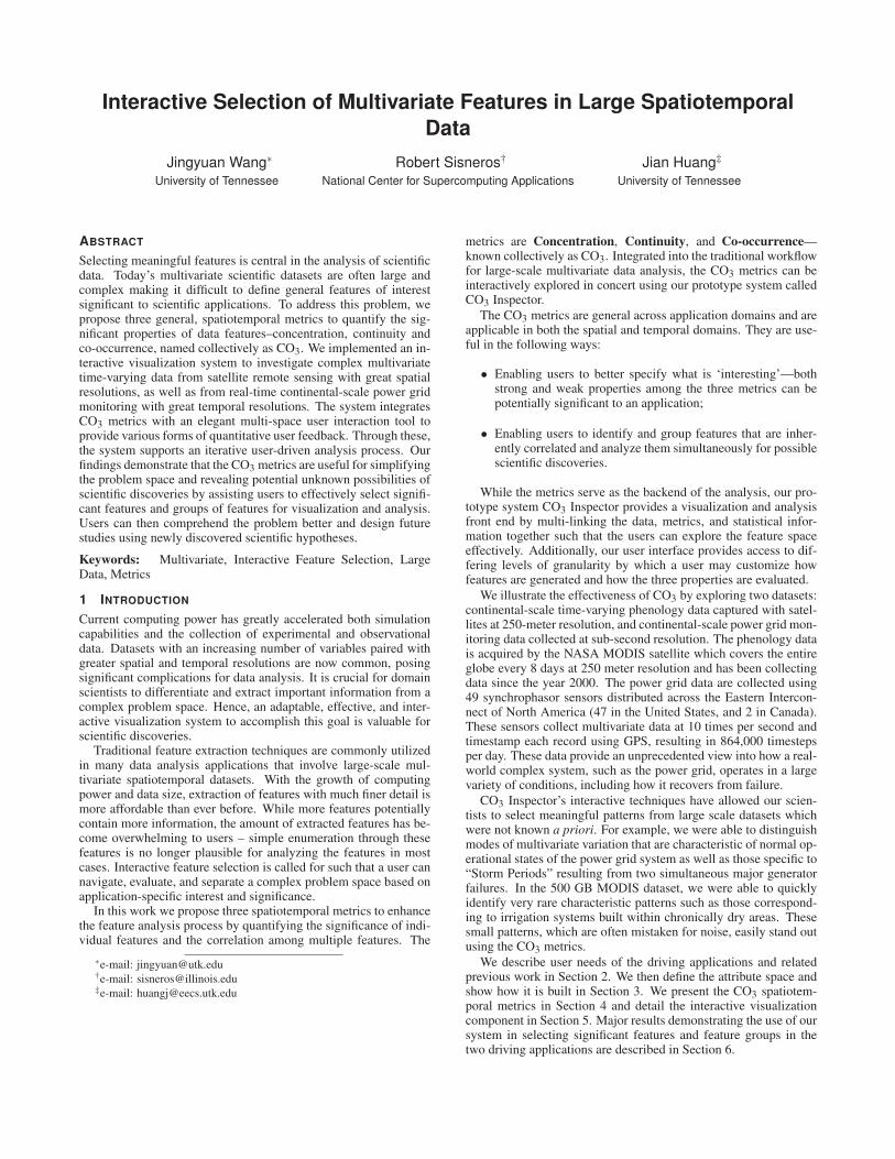
Figure 5: A highly continuous and concentrated feature in the MODISdata that captures areas of salt plains and white sands - The Bon-neville Salt Flats (1), White Sands National Monument (2), and othersalt flats (3) are highlighted. (Year 2000, 15km bin size)

(in red) is small but has a relatively high concentration and con-tinuity. The map in View D shows the geographic locations withthe phenological properties defined by the phenostate selected. Thethree labeled regions in the figure represent salt flats and areas withwhite sands. The Bonneville Salt Flats near the Great Salt Lake isthe most contiguous and concentrated feature. The other areas in-cluding the White Sands National Monument capture similar phe-nological properties— areas of the United States that remain a verywhite color year round (in contrast with snow, which is seasonal)and have absolutely no vegetation.

Example 2 (FNET): Similarly, in the FNET dataset, a smallnumber of features standing out from the majority in the metricspace represent possibilities of discovery. A tiny, highly concen-trated and continuous feature (in the top left of Figure 6(b) and thetop right of Figure 6(c)) proves to be unique after further study.The corresponding operation state dominantly appears across mostof the Eastern Interconnect but only within a very short period afterthe two generators’ temporary failure (shown by the solitary tall barin the temporal histogram). This feature has an exceptionally lowfrequency but a large phase angle shift. Its dominance indicatesthat this state is characteristic of the gradual process of the grid re-covering to normal operation. Further study of this would assist inunderstanding the recovery process and help technicians respondquickly to severe power grid failures.

(a)

(b) (c)

Figure 6: An example from the FNET data showing a highly concen-trated and continuous feature, with an exceptionally low frequencybut a large phase angle shift. Temporal histogram (a) shows this fea-ture is exclusive to a small window of time after the “Storm Period”.(1s bin size)

6.2 Selecting Significant Groups of Features

Selecting significant individual features can become overwhelmingfor a large number of features. As discussed earlier, simple enumer-ation is no longer plausible in actual analysis and discovering theimportant correlations among features in a complex feature spaceis very challenging. The co-occurrence graph layout of the CO3

Inspector, linked with the other metric views, enables users to navi-gate through the feature space, and select both interesting individualfeatures as well as interesting groups of features.

Example 1 (MODIS): Exploring the co-occurrence graph relat-ing to the salt flat phenostate mentioned above, we find a relatedfeature group spreading out sparsely over the whole continentalU.S. By further drilling down on some of the co-occurring phenos-tates, a set of small phenostates shows very interesting spatial dis-tribution and is illustrated in Figure 7. The three labeled areas in thefigure are representative of arid lands that contain significant greenareas because of human activity and irrigation. These clusters arephenologically similar to the salt plains in that they are regions witha severe lack of available water.

(a)

(b)

Figure 7: An example feature group in the MODIS data. The se-lection starts from the example feature of salt flats and white sands.After a series of navigation and selection refinement steps, users areable to discover such a feature group. These phenostates reside insome large irrigated lands in dry areas. (Year 2000, 15km bin size)

Example 2 (MODIS): Starting from the co-occurrence metric inthe MODIS dataset with a 5km bin size, we notice a feature groupin the co-occurrence graph which is highlighted in the spatial view(Figures 8(a) and 8(b)). It appears that this feature group repre-sents the outline of the Central California Valley and other areas inthe Southern Great Plains, both of which undergo rather irregulargrowing patterns due to the terrain of the Sierra Nevada mountainrange and the highly varied weather patterns in the southern part ofthe Great Plains. By looking at an earlier stage of the graph layoutconvergence process, as shown in Figures 9(b) and 9(d), we can seethat the original feature group is now expanded into two distinctareas. The top half of the group gives a near-exact outline of theCentral California Valley.

We iteratively adjust the bin size to 20km (Figures 8(c) and 8(d)).We notice that the group of clusters gets tighter. However, the twomain parts in the original group of features become separated whenthe bin size is 20km, leaving the Central California Valley directlyselectable without going back to the earlier layout process. In thisresult, with larger bin sizes, we were able to select structures be-longing to larger spatial scales.

Example 3 (FNET): With the FNET dataset, we can analyzethe uncommon event called a “Storm Period” by computing the co-occurrence graph composed solely of the features that occurred dur-ing that time (Figure 10). The co-occurrence graph layout clearlyreveals 6 characteristic groups that provide additional informationupon further examination. Figure 10(a) reveals that one group(highlighted in red) involves features with both high frequency vari-

(a) (b)

(c) (d)

Figure 8: An example feature group in the MODIS data. The spa-tial distribution a the feature group containing areas in the SouthernGreat Plains and the outline of the Central California Valley (Year2003, (a, b) 5km bin size, (c, d) 20km bin size).

ation and high voltage variation and occurred most frequently dur-ing the first half of the day (UTC time 00:43:12 to 08:52:48). Fig-ure 10(b) shows another feature group that had a heavier presencein the second half of the day (UTC time 12:00:00 to 21:07:12) andexhibited smaller variations in frequency but larger ones in voltage.As visualized by the parallel coordinate rendering in Figure 10(e)vs. Figure 10(f), the contrasting behavior could help to motivatefurther domain science research to explain the cause and progres-sion of a “Storm Period”.

Discussion: The feature groups identified in the above exam-ples show characteristic multivariate properties that might be sig-nificant to domain-specific users. However, without a proper tool,it is difficult to select these groups of features from the clutteredattribute space.

As an example, the first feature group representing salt flats andwhite sands contains 17 clusters, all of which are small with nodistinguishing traits in terms of concentration or continuity. Se-lecting individual features from among the whole population is notstraightforward. Even enumerating all features in the attribute space(223 clusters) would not help much in this case since each is toosimilar to the others to attract a user’s attention. //none of them isunique enough to attract the user’s attention. Also, these featuresmight be well hidden among other small features and mistakenlyconsidered to be noise. By selecting them, the spatial distributionreveals a meaningful and significant pattern.

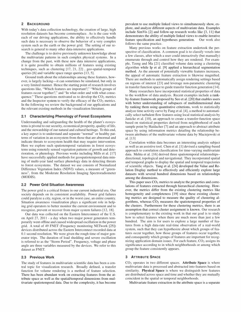
There are many existing approaches for multivariate feature vi-sualization. Using parallel coordinates, users are able to specifyranges for one or multiple variables to select a subset of all the fea-tures. Figure 11(b) is a parallel coordinates plot corresponding tothe first selected feature group shown in Figure 7. All features inthe same attribute space are plotted in orange and shown in Fig-ure 11(a). Here, the selected features share similar variation pat-terns while the actual values of the vegetation indices are not par-ticularly close to each other. In Figure 11(a), the multi-dimensionalcurves of all features do not show a clear structure or pattern toassist users in making a selection, as in Figure 11(b).

Similarly, Figures 11(c) and 11(d) demonstrate the advantage ofselecting a significant group of features using our tool. In these twofigures, the original features are colored in orange and the featuregroups selected using our tool are colored in red. Figures 11(c)and 11(d) correspond to the example feature group illustrated in

(a) (b)

(c) (d)

Figure 9: We expand the graph in Figure 8(b) and refine the selec-tion to two individual parts that initially appeared together. The areashowed on the top row is almost totally correlated to the Central Cal-ifornia Valley. (Year 2003, 5km bin size)

Figures 10(a) and 10(b), respectively. Additionally, we highlighttwo example selections of features using two different range queriesin the same plot (blueish color). The queries are conducted on fre-quency (11(c)) and frequency variation (11(d)) variable, based onthe exact distribution of the corresponding example feature group.In Figures 11(c) and 11(d), the total number of features is 1680.The queries on parallel coordinates results in selections of 1059 and684 features respectively while the selection using CO3 Inspectorcontains only 52 and 32 characteristically similar features. In bothcases, simple compound range queries could not reveal the patternsfound using our tool.

7 CONCLUSION AND DISCUSSION

CO3 represents a new possible solution to facilitate visual and in-teractive feature analysis and selection by developing quantitativemetrics that combine physical and attribute domains. Our capabil-ity to effectively select significant groups of features demonstratesthe power of the CO3 metrics in exposing previously unknown pos-sibilities to users. The feature selection capability we demonstrateis crucial as datasets consistently and quickly grow in size and com-plexity. CO3 metrics are especially useful to summarize physicalspace properties of features extracted from attribute space. Our useof coarse grained bins is general and novel for handling high res-olutioned spatial and temporal datasets. Our domain experts fromclimate modeling and power systems find CO3 metrics and the In-spector system to be useful for analyzing historical data. They wereintrigued by the feature groups discovered by the Inspect system,and expressed a perception of a high level of utility and future po-tential. Our work also has a few limitations. First, our methodrequires non-trivial parallel preprocessing. Next, the color schemewe employed was chosen out of convenience. Finally, our methodwould not offer significant benefit over previous methods, if thedataset is relatively manageable or the feature set is already wellunderstood.

8 ACKNOWLEDGEMENT

We thank Dr. Richard Mills and Forrest Hoffman of Oak Ridge Na-tional Laboratory for inspiring us to undertake this research topicand for their insightful and substantive feedback. We also thank Dr.Wesley Kendall of University of Tennessee for his help with refin-ing the scope of this work. Our work was supported in part by NSF

(a) (b)

(c) (d)

(e) (f)

Figure 10: Two example feature groups in the FNET data; both oc-curred in a “Storm Period”. Both are inherently correlated in termsof co-occurrence, but contain highly contrasting distribution patterns.(1s bin size)

Office of Cyber Infrastructure under ARRA-NSF-OCI-0906324,DOE SciDAC Ultrascale Visualization Institute (DOE DE-FC02-06ER25778), and by the Engineering Research Center Program ofNSF and DOE under NSF-EEC-1041877.

REFERENCES

[1] C.-K. Chen, C. Wang, K.-L. Ma, and A. Wittenberg. Static correla-

tion visualization for large time-varying volume data. In IEEE Pacific

Visualization Symposium, pages 27–34, 2011.

[2] H. Doleisch, M. Gasser, and H. Hauser. Interactive feature specifica-

tion for focus+context visualization of complex simulation data. In

VisSym, pages 239–248, 2003.

[3] H. Doleisch, M. Mayer, M. Gasser, P. Priesching, and H. Hauser. Inter-

active feature specification for simulation data on time-varying grids.

SimVis, pages 291–304, 2005.

[4] Z. Fang, T. Moller, G. Hamarneh, and A. Celler. Visualization and ex-

ploration of time-varying medical image data sets. In Proc. of Graph-

ics Interface, pages 281–288, 2007.

[5] M. Glatter, J. Huang, S. Ahern, J. Daniel, and A. Lu. Visualizing

temporal patterns in large multivariate data using modified globbing.

IEEE Trans. Vis. Comput. Graphics, 14(6):1467–1474, 2008.

[6] M. Hadwiger, F. Laura, C. Rezk-Salama, T. Hollt, G. Geier, and T. Pa-

bel. Interactive volume exploration for feature detection and quan-

tification in industrial ct data. IEEE Trans. Vis. Comput. Graphics,

14(6):1507–1514, 2008.

[7] M. Haidacher, D. Patel, S. Bruckner, A. Kanitsar, and M. Groller.

Volume visualization based on statistical transfer-function spaces. In

IEEE Pacific Visualization Symposium, pages 17–24, 2010.

[8] S. Ingram, T. Munzner, V. Irvine, M. Tory, S. Bergner, and T. Moller.

Dimstiller: Workflows for dimensional analysis and reduction. In

IEEE Symp. on Visual Analytics Sci. & Technology, pages 3–10, 2010.

[9] C. Y. Ip, A. Varshney, and J. JaJa. Hierarchical exploration of volumes

using multilevel segmentation of the intensity-gradient histograms.

IEEE Trans. Vis. Comput. Graphics, 18:2355–2363, 2012.

[10] H. Janicke, A. Wiebel, G. Scheuermann, and W. Kollmann. Multi-

field visualization using local statistical complexity. IEEE Trans. Vis.

Comput. Graphics, 13(6):1384–1391, 2007.

[11] J. Kehrer, F. Ladstadter, P. Muigg, H. Doleisch, A. Steiner, and

H. Hauser. Hypothesis generation in climate research with interac-

tive visual data exploration. IEEE Trans. Vis. Comput. Graphics,

14(6):1579–1586, 2008.

[12] R. Klump and J. Weber. Real-time data retrieval and new visualization

(a) (b)

(c) (d)

Figure 11: Traditional parallel coordinates plots of example featuregroups (rendered with the other features in the same attribute spacein different colors): (a, b) Figure 7, (c) Figure 10(a), (d) Figure 10(b).The features that selected using CO3 Inspector are colored in red.The features selected by specifying variable ranges (c and d) areplotted in bluish color. The rest are colored in orange.

techniques for the energy industry. In Proc. of the Annual Hawaii Int.

Conference on System Sciences, pages 712–717, 2002.

[13] R. Maciejewski, Y. Jang, I. Woo, H. Janicke, K. Gaither, and D. Ebert.

Abstracting attribute space for transfer function exploration and de-

sign. IEEE Trans. Vis. Comput. Graphics, PP(99):1, 2012.

[14] R. Maciejewski, I. Woo, W. Chen, and D. Ebert. Structuring feature

space: A non-parametric method for volumetric transfer function gen-

eration. IEEE Trans. Vis. Comput. Graphics, 15(6):1473–1480, 2009.

[15] S. Martin, W. M. Brown, R. Klavans, and K. W. Boyack. Openord:

an open-source toolbox for large graph layout. In Proc. SPIE 7868,

Visualization and Data Analysis, 2011.

[16] S. Mehta, S. Parthasarathy, and R. Machiraju. Visual exploration of

spatio-temporal relationships for scientific data. In IEEE Symposium

on Visual Analytics Science And Technology, pages 11–18, 2006.

[17] R. T. Mills, F. M. Hoffman, J. Kumar, and W. W. Hargrove. Clus-

ter analysis-based approaches for geospatiotemporal data mining of

massive data sets for identification of forest threats. Procedia CS,

4:1612–1621, 2011.

[18] T. J. Overbye. Transmission system visualization for the smart grid

(panel summary). In Proc. of Power Systems Conference and Exposi-

tion, pages 1–2, 2009.

[19] A. Rosenberg and J. Hirschberg. V-measure: A conditional entropy-

based external cluster evaluation measure. In Proc. of Joint Conf. on

Empirical Methods in Natural Language Processing and Computa-

tional Natural Language Learning, pages 410–420, 2007.

[20] J. Seo and B. Shneiderman. A rank-by-feature framework for interac-

tive exploration of multidimensional data. Information Visualization,

4(2):99–113, 2005.

[21] F.-Y. Tzeng and K.-L. Ma. A Cluster-Space Visual Interface for Arbi-

trary Dimensional Classification of Volume Data . In Proc. of VisSym,

pages 17–24, 2004.

[22] J. Wei, H. Yu, J. Chen, and K.-L. Ma. Parallel clustering for visu-

alizing large scientific line data. In IEEE Symposium on Large Data

Analysis and Visualization, pages 47–55, 2011.

[23] I. Woo, R. Maciejewski, K. P. Gaither, and D. S. Ebert. Feature-driven

data exploration for volumetric rendering. IEEE Trans. Vis. Comput.

Graphics, 18(10):1731–1743, 2012.

[24] J. Yang, D. Hubball, M. Ward, E. Rundensteiner, and W. Ribarsky.

Value and relation display: Interactive visual exploration of large data

sets with hundreds of dimensions. IEEE Trans. Vis. Comput. Graph-

ics, 13(3):494–507, 2007.

[25] Y. Zhang, P. Markham, T. Xia, L. Chen, Y. Ye, Z. Wu, Z. Yuan,

L. Wang, J. Bank, J. Burgett, R. Conners, and Y. Liu. Wide-area fre-

quency monitoring network (fnet) architecture and applications. IEEE

Trans. Smart Grid, 1(2):159–167, 2010.