Masteruppsats i matematisk statistikMaster Thesis in Mathematical Statistics

Interest Rate Derivatives: An analysis ofinterest rate hybrid products

Taurai Chimanga

Masteruppsats 2011:3Matematisk statistikMars 2011

www.math.su.se

Matematisk statistikMatematiska institutionenStockholms universitet106 91 Stockholm

Mathematical StatisticsStockholm UniversityMaster Thesis 2011:3

http://www.math.su.se

Interest Rate Derivatives: An analysis of

interest rate hybrid products

Taurai Chimanga∗

March 2011

Abstract

The globilisation phenomena is causing an increasing interaction

between different markets and sectors. This has led to the evolution

of derivative instruments from ”single asset” instruments to complex

derivatives that have underlying assets from different markets, sectors

and sub-sectors. These are the so-called hybrid products that have

multi-assets as underlying instruments. This article focuses on inter-

est rate hybrid products. In this article an analysis of the application

of stochastic interest rate models and stochastic volatility models in

pricing and hedging interest rate hybrid products will be explored.

∗Postal address: Mathematical Statistics, Stockholm University, SE-106 91, Sweden.

E-mail:t chimanga@yahoo.com . Supervisor: Thomas Hoglund.

“ There is only one good, knowledge, and one evil, ignorance.”Socrates

I dedicate this thesis to my grandmother. Thank you for being my pillarof strength.

2

Contents

1 Introduction 4

2 A Primer on Interest Rate Products 52.1 Term Structure of Interest Rates . . . . . . . . . . . . . . . . 52.2 Combining Asset Classes . . . . . . . . . . . . . . . . . . . . . 7

3 Stochastic Interest Rates 83.1 Deterministic vs Stochastic Rates of Interest . . . . . . . . . . 83.2 Affine Term Structure . . . . . . . . . . . . . . . . . . . . . . 93.3 Pricing a Cap . . . . . . . . . . . . . . . . . . . . . . . . . . . 103.4 Calibration . . . . . . . . . . . . . . . . . . . . . . . . . . . . 103.5 Analysing the Rate-Stock Correlation . . . . . . . . . . . . . . 103.6 Pricing the Hybrid . . . . . . . . . . . . . . . . . . . . . . . . 12

3.6.1 Analytical Solution . . . . . . . . . . . . . . . . . . . . 123.7 Hedging . . . . . . . . . . . . . . . . . . . . . . . . . . . . . . 13

4 Stochastic Volatility 144.1 Change of Numeraire . . . . . . . . . . . . . . . . . . . . . . . 154.2 Pricing . . . . . . . . . . . . . . . . . . . . . . . . . . . . . . . 164.3 Hedging . . . . . . . . . . . . . . . . . . . . . . . . . . . . . . 24

5 Hedging Accuracy Tests 255.1 Conclusion . . . . . . . . . . . . . . . . . . . . . . . . . . . . . 30

6 Data 31

3

1 Introduction

Globilisation has created an increasing interaction between different mar-kets, sectors and sub-sectors. It is typical that a single investor might havesimultaneous open position in different markets or asset classes. This hasprompted the financial engineering of complex financial products called hy-brid products. A hybrid product is a financial instrument whose payout islinked to underlyings belonging to different, but usually correlated, markets.The focus of this paper is on interest rate hybrid products. In this article ananalysis of the application of stochastic interest rate models and stochasticvolatility models in pricing and hedging interest rate hybrid products will beexplored.

In this paper we keep in mind that a complicated model is harder toimplement in practice. We will thus analyse the impact of using stochasticinterest rates and stochastic volatility on an interest rate hybrid product.These models will be dealt with in a manner to keep the problem tractable.Stochastic interest rates will be introduced first and thereafter stochasticvolatility will be included. We will thus compare how the models performbased on how well they hedge the hybrid.

The rest of this paper will be arranged as follows. Section 2 will give abrief introduction of the interest rate products. Section 3 will look at theimpact of stochastic interest rates in pricing hybrid products. The specifichybrid product to be analysed in this article will be introduced and otherclasses that can be combined with interest rates in creating hybrid productswill be discussed. Section 4 will look at the inclusion of stochastic volatilitymodels in the hybrid setting. Section 5 compares how the models performbased on how well they hedge the hybrid and will give concluding remarks.

4

2 A Primer on Interest Rate Products

In pricing derivatives, modelling is usually done under a risk neutral measureor a martingale measure Q. Under Q, the standard numeraire is the moneyaccount. The dynamics of the money account are governed by the evolutionof the interest rate. Thus in valuing any contingent claim, interest rates playa vital role. We take for instance the price of a call option on a stock:

Pricecall(t) = e−r(T−t)EQ[(ST −K)+|Ft] (1)

where r represents the interest rate.If the derivative has the interest rate as the underlying eg. options on

bonds, swaptions and captions, the modelling of the interest rate becomesincreasingly important. As interest rate derivative prices are sensitive to thepricing of interest rate dependant assets, it would thus not make much senseto use a model to price the derivatives which hardly prices the underlyingassets accurately. The simplest interest rate product is a zero coupon bondwhich pays its full face value at maturity T . The price of a zero coupon bondat time t, P (t, T ), is given by

P (t, T ) = e−R(t,T )(T−t) (2)

where R(t, T ) is the continuously compounded spot rate.

2.1 Term Structure of Interest Rates

We try to model an arbitrage-free family of zero coupon bonds. We assumethat under the objective probability measure P, the short rate process followsthe SDE

drt = µ(t, rt)dt + σ(t, rt)dW (3)

We assume the existence of an arbitrage free market and a market for T-bonds for every choice of T. Furthermore, we assume that the price of aT-bond has the form

P (t, T ) = F (t, rt, T ) (4)

where F is a smooth function of three variables with simple boundary con-dition

F (T, r, T ) = 1 ∀ r (5)

5

In an arbitrage free bond market, F must satisfy the term structure equation:

Ft + (µ− σλ)Fr +1

2σ2Frr − rF = 0 (6)

F (T, r, T ) = 1. (7)

λ is exogenous and represents the market price of risk whereas Fr denotesthe partial derivative of F with respect to variable r. The Feynman-Kacrepresentation of F from (6) and (7) implies that the T-bond prices aregiven by

F (t, r, T ) = EQ[e−

∫ Tt rs ds

](8)

where Q denotes that the expectation is taken under the martingale measurewith the short rate following the SDE

drs = (µ− λσ)ds + σdW (9)

As there are many interest rate products, they are combined to form theyield curve usually expressed in terms of zero coupon bond prices. Struc-tured interest products are usually replicated with simpler instruments. Ifthe combination of the simpler instruments mimics the payoff of the struc-tured product then under standard arbitrage arguments, the price of thestructured product must be equal to the value of the combination of thesimpler instruments. Other complex structures can not be replicated withsimpler instruments thus numerical procedures are used for their valuations.

We will look at an example of an interest rate product called a cap. Acap is a portfolio of call options used to protect the holder from a rise in theinterest rate. Each of the individual options constituting a cap is known as acaplet. At the exercise dates, if the reference rate rises above the strike price,the holder receives the difference between the strike price and the referencerate on the succesive coupon date.

As a cap is a portfolio of caplets, its value is equal to the value of thecaplets. If the ith caplet runs from Ti−1 to Ti, exercise decision is made ondate Ti−1 and the payment is received on date Ti. Assuming that the refer-ence rate is the LIBOR, K represents the strike price and δi represents theday count fraction of the ith period. The value of the ith caplet as seen onits exercise date is

ci(Ti−1) = P (Ti−1, Ti)δi

(LIBORi −K

)+(10)

which is equivalent to a European call option on the LIBOR struck at K.

6

2.2 Combining Asset Classes

Interest rate hybrid products have claims which are contingent upon move-ments in the interest rate and other asset classes. Although interest ratehybrids can be constructed with more than two asset classes, we restrict ouranalysis to only two asset classes. The hybrid we will consider will thus de-pend on interest rates and another asset class from either equity, inflation,foreign currency exchange or credit.

In this article we will look at a particular hybrid product which has acoupon payment similar to that of a caplet. We look at the hybrid best-ofproducts, which at time Ti pays coupons of the form

max{irate, a · (VTi/VTi−1

− 1)} (11)

where a represents the participation rate, irate represents the interest ratefor the coupon period eg. 3 month LIBOR, determined at time Ti−1 and Vt

represents the price of another asset class other than interest rates at timet. We are interested in analysing the properties of this hybrid product underdifferent assumptions. We assume that the hybrid will pay coupons quarterlyie δi = 0.25. We will use the equity class for V , 100% participation rate andthe 3 month LIBOR rate for irate for the rest of this article. As the interestcomponent is known at Ti−1 we can simplify the coupon payment at Ti as

max{δiLIBORi, STi

/STi−1− 1

}(12)

7

3 Stochastic Interest Rates

3.1 Deterministic vs Stochastic Rates of Interest

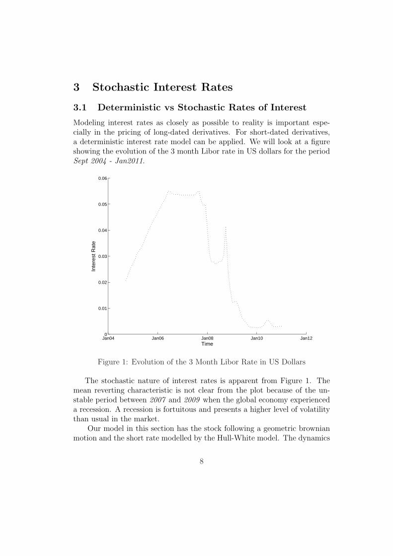
Modeling interest rates as closely as possible to reality is important espe-cially in the pricing of long-dated derivatives. For short-dated derivatives,a deterministic interest rate model can be applied. We will look at a figureshowing the evolution of the 3 month Libor rate in US dollars for the periodSept 2004 - Jan2011.

Jan04 Jan06 Jan08 Jan10 Jan120

0.01

0.02

0.03

0.04

0.05

0.06

Time

Inte

rest

Rat

e

Figure 1: Evolution of the 3 Month Libor Rate in US Dollars

The stochastic nature of interest rates is apparent from Figure 1. Themean reverting characteristic is not clear from the plot because of the un-stable period between 2007 and 2009 when the global economy experienceda recession. A recession is fortuitous and presents a higher level of volatilitythan usual in the market.

Our model in this section has the stock following a geometric brownianmotion and the short rate modelled by the Hull-White model. The dynamics

8

for the stock and the short-rate are:

dSt = µtStdt + σst StdW s

t (13)

drt = (θt − κtrt)dt + σrt dW r

t (14)

where 〈dW rt , dW s

t 〉 = ρdt

3.2 Affine Term Structure

According to [4], if the term structure {p(t, T ); 0 ≤ t ≤ T, T > 0} has theform

p(t, T ) = V (t, rt, T ) (15)

where V has the form

V (t, rt, T ) = eA(t,T )−B(t,T )rt (16)

and where A and B are deterministic functions, then the model is said topossess the affine term structure. We consider the Hull-White with constantvolatility parameters, κt = κ and σr

t = σr. According to [4], if the drift andvolatility parameters for the short rate are time independent, a necessarycondition for the existence of an affine term structure is that the drift andthe volatility are affine in r. This implies that the Hull-White model withconstant volatility parameters has an affine term structure with bond pricesgiven by

p(t, T ) = eA(t,T )−B(t,T )rt ; (17)

where

B(t, T ) =1

κ

{1− e−κ(T−t)

}(18)

A(t, T ) =

∫ T

t

{1

2σrB2(t, T )− θsB(s, T )

}(19)

The yield curve is inverted by choosing θ such that the model matches initialbond prices. Choosing θ is equivalent to specifying a martingale measureas we have different martingale measures for different choices of the marketprice of risk, λ. The theoretical bond prices using the martingale measure Qare given by

p(t, T ) =p∗(0, T )

p∗(0, t)exp

{B(t, T )f ∗(0, t)− σ2

r

4κB2(t, T )(1− e−2κt)−B(t, T )rt

}

(20)

9

where variables with a superscript * are observed from the market.

3.3 Pricing a Cap

We use the affine term structure to price a cap. The value of a cap is equalto the value of the caplets. The ith LIBOR is given by

Li =1

δi

(1

P (Ti−1, Ti)− 1

)(21)

The value of the ith caplet as seen on its exercise date is therefore:

ci(Ti−1) = P (Ti−1, Ti)δi(Li −K)+ (22)

ci(Ti−1) = (1− P (Ti−1, P (Ti))(1 + Kδi))+ (23)

and using (20)

⇒ ci(Ti−1) =

(1− (1 + Kδi)

p∗(0, Ti)

p∗(0, Ti−1)exp

{B(Ti−1, Ti)f

∗(0, Ti−1)

− σ2r

4κB2(Ti−1, Ti)(1− e−2κTi−1)−B(Ti−1, Ti)rTi−1

})+

(24)

where δi is the day count fraction corresponding to the ith LIBOR period.

3.4 Calibration

Calibration is the process of determining the parameters that are used inthe term structure model. In the Hull-White model, the parameters to bedetermined are κ and σr

t . The procedure is to choose the parameters suchthat the implementation of the term structure model replicates, as muchas possible, liquid interest rate dependant instruments like floors, caps andswaptions. Usually the prices or volatilities of the options that are used tohedge the option in question are used for the calibration.

3.5 Analysing the Rate-Stock Correlation

Figure 2 does not show any relationship between the monthly 3M LIBORrate and the monthly stock return between Sept 2004 - Jan 2011. However,low interest rates (close to zero) on the graph are consistent with the recoveryof the global economy from the recession. We test the correlation between

10

Jan04 Jan06 Jan08 Jan10 Jan12−0.3

−0.2

−0.1

0

0.1

0.2

0.3

0.4

Time

Inte

rest

Rat

e/S

tock

Ret

urn

Monthly US 3m Libor RateMonthly Google Stock Returns

Figure 2: Plot showing 3M Libor Rate and Google Stock Returns

the interest rate and the stock return. The p-values for testing the nullhypothesis that there is no correlation between the stock return and the 3MLIBOR rate against the alternative that there is a non-zero correlation areshown below.

method correlation coefficient p valuePearson -0.0274 0.8130

Spearman -0.0295 0.7992Kendall -0.0195 0.8054

The p-values are too large, they are À 0.05 and thus for all the methods,we fail to reject the null hypothesis.

11

3.6 Pricing the Hybrid

3.6.1 Analytical Solution

Our hybrid has call options embedded in it and thus we will price it as aportfolio of forward starting call options. The ith coupon payment made attime Ti, with exercise decision made at Ti−1 valued at time t0 is:

Πt0 = EQ[e−

∫ Tit0

rsdsmax

{δiLi,

STi

STi−1

− 1

}∣∣∣∣Ft0

](25)

Πt0 = EQ[e−

∫ Ti−1t0

rsdsEQ[e− ∫ Ti

Ti−1rsds

max

{δiLi,

STi

STi−1

− 1

}∣∣∣∣FTi−1

]∣∣∣∣Ft0

]

(26)

We first deal with the inner expectation which using (21) simplifies to

EQ[e− ∫ Ti

Ti−1rsds

(δiLi + max

{0,

STi

STi−1

− 1

P (Ti−1, Ti)

})∣∣∣∣FTi−1

](27)

using that STi= STi−1

e∫ Ti

Ti−1rsds− 1

2σ2(Ti−Ti−1)+σ(WTi

−WTi−1)(27) becomes

EQ[P (Ti−1, Ti)max

{0, e

∫ TiTi−1

rsds− 12σ2(Ti−Ti−1)+σ(WTi

−WTi−1) − 1

P (Ti−1, Ti)

}∣∣∣∣FTi−1

]

+ 1− P (Ti−1, Ti) (28)

=EQ[max

{0, e−

12σ2(Ti−Ti−1)+σ(WTi

−WTi−1) − 1

}∣∣∣∣FTi−1

]+ 1− P (Ti−1, Ti)

(29)

=Call(S = 1, K = 1, σ, r = 0, τ = Ti − Ti−1) + 1− P (Ti−1, Ti) (30)

Call(S = 1, K = 1, σ, r = 0, τ = Ti − Ti−1) is a call option valued in a worldwith zero interest rate. The volatility of the underlying is the unknown inputand thus it will determine the price of the option. The call option is struckat the money thus using the Black Scholes formula we get the value of thisoption as:

Call(S = 1, K = 1, σ, r = 0, τ = Ti − Ti−1) = N(d+)−N(d−) (31)

where:N(·) is the cumulative standard normal distribution function;

12

d+ =(log(S/K) + 0.5σ2τ

)/(σ

√τ)

d− = d+ − σ√

τ

Inserting the inner expectation back to (26) yields:

Πt0 =EQ[e−

∫ Ti−1t0

rsds

{N(d+)−N(d−) + 1− P (Ti−1, Ti)

}∣∣∣∣Ft0

]

Πt0 =P (t0, Ti−1)

{N(d+)−N(d−) + 1

}− P (t0, Ti) (32)

We notice that P (t0, Ti−1) and P (t0, Ti) are observed from the market andthus the pricing of the hybrid is invariant under stochastic interest rates.The volatility of the underlying will thus determine the price of the hybrid.

3.7 Hedging

In this section, we let N(d+)−N(d−) + 1 = c. The interest rate is the onlysource of risk and thus to make our portfolio delta neutral, we have to hedgeagainst interest rate movements. We use a T ∗ bond to hedge the interestrate risk where T ∗ > Ti. We thus seek to determine how many T ∗ bonds werequire to hedge the interest rate delta. Let x be the number of T ∗ bondsrequired.

∂

∂r

{cP (t0, Ti−1)− P (t0, Ti)

}=

∂

∂r

{xP (t0, T

∗)}

(33)

We know that P (t, T ) = exp(−r(T − t)) thus we get that

x =∂

∂r

{cP (t0, Ti−1)− P (t0, Ti)

}/∂

∂r

{P (t0, T

∗)}

(34)

= −{(

Ti − t0)P (t0, Ti)− c(Ti−1 − t0)P (t0, Ti−1)

}/{(T ∗ − t0)P (t0, T

∗)}

(35)

13

4 Stochastic Volatility

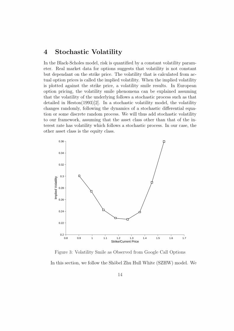
In the Black-Scholes model, risk is quantified by a constant volatility param-eter. Real market data for options suggests that volatility is not constantbut dependant on the strike price. The volatility that is calculated from ac-tual option prices is called the implied volatility. When the implied volatilityis plotted against the strike price, a volatility smile results. In Europeanoption pricing, the volatility smile phenomena can be explained assumingthat the volatility of the underlying follows a stochastic process such as thatdetailed in Heston(1993)[2]. In a stochastic volatility model, the volatilitychanges randomly, following the dynamics of a stochastic differential equa-tion or some discrete random process. We will thus add stochastic volatilityto our framework, assuming that the asset class other than that of the in-terest rate has volatility which follows a stochastic process. In our case, theother asset class is the equity class.

0.8 0.9 1 1.1 1.2 1.3 1.4 1.5 1.6 1.70.2

0.22

0.24

0.26

0.28

0.3

0.32

0.34

0.36

Strike/Current Price

Impl

ied

Vol

atili

ty

Figure 3: Volatility Smile as Observed from Google Call Options

In this section, we follow the Shobel Zhu Hull White (SZHW) model. We

14

present a slight change of notation to the dynamics of the stock and interestrate processes and assume that the volatility process follows an Ornstein-Uhlenbeck process. The dynamics for the stock process, volatility processand interest rate process are as follows:

dSt = µtStdt + vtStdW st (36)

dvt = κ[ω − vt]dt + σvdW vt (37)

drt = (ζ − ηtrt)dt + σrdW rt (38)

〈dW vt , dW s

t 〉 = ρsvdt

〈dW rt , dW s

t 〉 = ρrsdt

〈dW vt , dW r

t 〉 = ρrvdt

(39)

4.1 Change of Numeraire

We change the numeraire to a T-bond and thus change our measure from Qto a T-forward measure, QT . By changing the numeraire, we hope to loseone variable and be left with two variables to deal with. We introduce theforward price

Ft =St

P (t, T )(40)

Recalling the Hull-White affine term structure framework given in (20), thedynamics for the discount process under Q are given by

dP = rtPdt− σrB(t, T )PdW rt (41)

Applying Ito’s lemma to (40) yields

dF = (σ2rB

2r (t, T ) + ρrsvtσrB(t, T ))Fdt + vtFdW s

t + σrB(t, T )FdW rt (42)

Ft is a martingale under QT and thus we have the following transformationsfrom the Q measure to the QT measure:

dW rt 7→ dW T

r (t)− σrB(t, T )dt

dW st 7→ dW T

s (t)− ρrsσrB(t, T )dt

dW vt 7→ dW T

v (t)− ρrvσrB(t, T )dt

15

Thus under QT , vt and Ft can be written as

dv(t) = κ[ω − ρrvσrσvB(t, T )

κ− vt]dt + σvdW T

v (t) (43)

dF (t) = vtFdW Ts (t) + σrB(t, T )FdW T

r (t) (44)

We can simplify (44) by using a log transformation and switching fromdW T

r (t) and dW Ts (t) to dW T

F (t). We let y(t) = log(F (t)) and use Ito’s lemmato get:

dv(t) = κ[θ − vt]dt + σvdW Tv (t) (45)

dy(t) = −1

2ϕ2

F (t)dt + ϕF (t)dW TF (t) (46)

with

ϕ2F (t) = v2 + 2ρrsvtσrB(t, T ) + σ2

rB2(t, T )

θ = ω − ρrvσrσvB(t, T )

κ(47)

4.2 Pricing

According to the Meta Theorem in [4], a market is incomplete if the numberof random sources in the model is greater than the number of traded assets.This implies that the model with stochastic volatility presents an incompletemarket as there are at least two driving Weiner processes and only one tradedasset. We now seek for a characteristic function for the forward log-assetprice. We apply the Feynman-Kac theorem which transforms the probleminto solving a PDE.

According to the the Feynman-Kac theorem, the characteristic functiongiven by

f(t, y, v) = EQT [exp(iuy(T ))|Ft

](48)

is the solution to the PDE

0 = ft − 1

2ϕ2

F (t)fy + κ(θ − v)fv +1

2ϕ2

F (t)fyy (49)

+ (vσvρsv + ρrvσvσrB(t, T ))fyv +1

2σ2

vfvv

f(T, y, v) = exp(iuy(T )) (50)

The solution to this problem is presented in [15]. We present the solutionhere and for proof, the reader is refered to the [15].

16

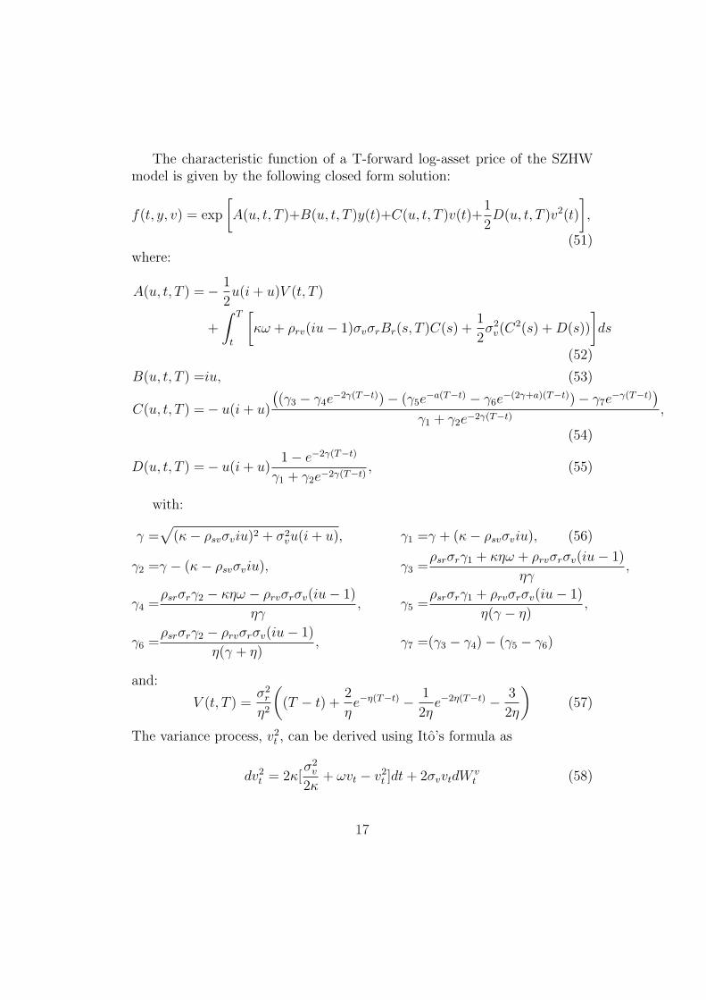
The characteristic function of a T-forward log-asset price of the SZHWmodel is given by the following closed form solution:

f(t, y, v) = exp

[A(u, t, T )+B(u, t, T )y(t)+C(u, t, T )v(t)+

1

2D(u, t, T )v2(t)

],

(51)where:

A(u, t, T ) =− 1

2u(i + u)V (t, T )

+

∫ T

t

[κω + ρrv(iu− 1)σvσrBr(s, T )C(s) +

1

2σ2

v(C2(s) + D(s))

]ds

(52)

B(u, t, T ) =iu, (53)

C(u, t, T ) =− u(i + u)

((γ3 − γ4e

−2γ(T−t))− (γ5e−a(T−t) − γ6e

−(2γ+a)(T−t))− γ7e−γ(T−t)

)

γ1 + γ2e−2γ(T−t),

(54)

D(u, t, T ) =− u(i + u)1− e−2γ(T−t)

γ1 + γ2e−2γ(T−t), (55)

with:

γ =√

(κ− ρsvσviu)2 + σ2vu(i + u), γ1 =γ + (κ− ρsvσviu), (56)

γ2 =γ − (κ− ρsvσviu), γ3 =ρsrσrγ1 + κηω + ρrvσrσv(iu− 1)

ηγ,

γ4 =ρsrσrγ2 − κηω − ρrvσrσv(iu− 1)

ηγ, γ5 =

ρsrσrγ1 + ρrvσrσv(iu− 1)

η(γ − η),

γ6 =ρsrσrγ2 − ρrvσrσv(iu− 1)

η(γ + η), γ7 =(γ3 − γ4)− (γ5 − γ6)

and:

V (t, T ) =σ2

r

η2

((T − t) +

2

ηe−η(T−t) − 1

2ηe−2η(T−t) − 3

2η

)(57)

The variance process, v2t , can be derived using Ito’s formula as

dv2t = 2κ[

σ2v

2κ+ ωvt − v2

t ]dt + 2σvvtdW vt (58)

17

which can be written as the familiar square root process [used by Cox, In-gersoll, and Ross(1985)]

dv∗t = κ∗[θ∗ − v∗t ]dt + σ∗v√

v∗t dW vt (59)

with

v2t = v∗t , κ∗ = 2κ

θ∗ =σ2

v

2κ+ ωvt, σ∗v = 2σv (60)

where κ∗ is called the “speed of mean reversion”,√

θ∗ the “long vol”, σ∗v the“vol of vol” and the initial value v∗0 the “short vol”.According to [12] thevol of vol and the correlation can be thought as the parameters responsiblefor the skew whereas the other parameters control the term structure of themodel. We can see from (59) that the Heston model is as special case of ourmodel.

When pricing our hybrid, we have to price it as a forward starting option.We follow the method proposed by [8]. The value of the hybrid at time t0 isgiven by:

Πt0 = P (t, Ti)EQT

[max

{δLi,

STi

STi−1

− 1

}∣∣∣∣Ft0

](61)

= P (t0, Ti−1)EQT

[P (Ti−1, Ti)E

QT

[max

{δLi,

ST

STi−1

− 1

}∣∣∣∣FTi−1

∣∣∣∣]Ft0

]

(62)

= P (t0, Ti−1)EQT

[P (Ti−1, Ti)E

QT

[δLi +

{STi

STi−1

− 1

P (Ti−1, Ti)

}+∣∣∣∣FTi−1

]∣∣∣∣Ft0

]

(63)

= P (t0, Ti−1)EQT

[P (Ti−1, Ti)δLi + P (Ti−1, Ti)E

QT

{STi

STi−1

− 1

P (Ti−1, Ti)

}+∣∣∣∣FTi−1

]∣∣∣∣Ft0

]

(64)

= P (t0, Ti−1)EQT

[P (Ti−1, Ti)δLi

∣∣∣∣Ft0

](65)

+ P (t0, Ti)EQT

[EQT

[{STi

STi−1

− 1

P (Ti−1, Ti)

}+∣∣∣∣FTi

]∣∣∣∣Ft0

](66)

18

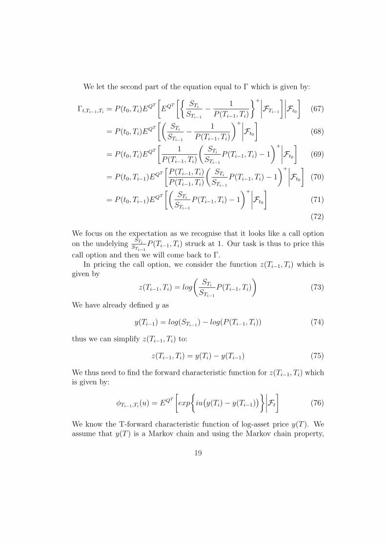
We let the second part of the equation equal to Γ which is given by:

Γt,Ti−1,Ti= P (t0, Ti)E

QT

[EQT

[{STi

STi−1

− 1

P (Ti−1, Ti)

}+∣∣∣∣FTi−1

]∣∣∣∣Ft0

](67)

= P (t0, Ti)EQT

[(STi

STi−1

− 1

P (Ti−1, Ti)

)+∣∣∣∣Ft0

](68)

= P (t0, Ti)EQT

[1

P (Ti−1, Ti)

(STi

STi−1

P (Ti−1, Ti)− 1

)+∣∣∣∣Ft0

](69)

= P (t0, Ti−1)EQT

[P (Ti−1, Ti)

P (Ti−1, Ti)

(STi

STi−1

P (Ti−1, Ti)− 1

)+∣∣∣∣Ft0

](70)

= P (t0, Ti−1)EQT

[(STi

STi−1

P (Ti−1, Ti)− 1

)+∣∣∣∣Ft0

](71)

(72)

We focus on the expectation as we recognise that it looks like a call option

on the undelyingSTi

STi−1P (Ti−1, Ti) struck at 1. Our task is thus to price this

call option and then we will come back to Γ.In pricing the call option, we consider the function z(Ti−1, Ti) which is

given by

z(Ti−1, Ti) = log

(STi

STi−1

P (Ti−1, Ti)

)(73)

We have already defined y as

y(Ti−1) = log(STi−1)− log(P (Ti−1, Ti)) (74)

thus we can simplify z(Ti−1, Ti) to:

z(Ti−1, Ti) = y(Ti)− y(Ti−1) (75)

We thus need to find the forward characteristic function for z(Ti−1, Ti) whichis given by:

φTi−1,Ti(u) = EQT

[exp

{iu

(y(Ti)− y(Ti−1)

)}∣∣∣∣Ft

](76)

We know the T-forward characteristic function of log-asset price y(T ). Weassume that y(T ) is a Markov chain and using the Markov chain property,

19

y(Ti−1) and y(Ti) are independent given that ∃ t∗ where Ti−1 < t∗ < Ti s.ty(t∗) exists. We assume that such a t∗ exists. A characteristic function forthe difference of two independent random variables x and y is given by:

φx−y(u) = φx(u)φy(−u) (77)

Thus the forward characteristic function for z(Ti−1, Ti) is given by:

φTi−1,Ti(u) = EQT

[exp

{iuy(Ti)

}∣∣∣∣Ft

]EQT

[exp

{− iuy(Ti−1)

}∣∣∣∣Ft

](78)

= f(Ti, y, v, u)f(Ti−1, y, v,−u) (79)

Once we have the forward characteristic function, we use Fourier FastTranform(FFT) method proposed by [6]. We use a value of 1.25 for α forthe modified call option given by:

cT (k) = exp(αk)P (t0, Ti)EQT

[(eZ(Ti−1,Ti) − ek

)+](80)

wherek = log(K).

The transform of the call as given by [8] is:

ψ(t0, Ti−1, Ti) = P (t0, T )φTi−1,Ti

(u− (α + 1)i)

(α + iu)(α + 1 + iu)(81)

We can thus calculate the price of the forward starting call using theinverse FFT. Let Cfwd(t0, Ti−1, Ti) denote the price of this forward startingoption. Returning to Γ, we get that:

Γt0,Ti−1,Ti= P (t0, Ti−1)C

fwd(t0, Ti−1, Ti) (82)

In Section 3, we showed that

P (t, Ti−1)EQT

[P (Ti−1, Ti)δLi

∣∣∣∣Ft

]= P (t0, Ti−1)− P (t0, Ti) (83)

thus the price of the hybrid is given by:

Πt = P (t0, Ti−1)

{1 + Cfwd(t0, Ti−1, Ti)

}− P (t0, Ti) (84)

We note that the prices of the bonds P (t0, Ti−1) and P (t0, Ti) are observedfrom the market.

20

0.51

1.52

2.53

0.8

0.9

1

1.1

1.2

1.30.4

0.6

0.8

1

1.2

1.4

1.6

1.8

Maturity

Volatility Surface for our model with starting time = .25

strike

Impl

ied

Vol

atili

ty

Figure 4: Volatility Surface for our Model with Ti−1 = .25yr, S0 = 1, V0 =.2, κ = 2, η = 2, ω = .08, σr = .02, ρsv = .5, ρsr = .5, ρrv = .5, r0 = .02

21

0.8 0.85 0.9 0.95 1 1.05 1.1 1.15 1.2 1.250.9

1

1.1

1.2

1.3

1.4

1.5

Moneyness

Impl

ied

Vol

atili

ty

Skew Volatility for our model with starting time = .25

Figure 5: Skew Volatility for our Model with: Ti−1 = .25yr, S0 = 1, V0 =.2, κ = 2, η = 2, ω = .08, σr = .02, ρsv = .5, ρsr = .5, ρrv = .5, r0 = .02

22

0.51

1.52

2.53

0.8

0.9

1

1.1

1.2

1.30.7

0.8

0.9

1

1.1

1.2

1.3

1.4

1.5

1.6

Maturity

Volatility Surface for our model with ω = .16

strike

Impl

ied

Vol

atili

ty

Figure 6: Volatility Surface for our Model with Ti−1 = .25yr, S0 = 1, V0 =.2, κ = 2, η = 2, ω = .16, σr = .02, ρsv = .5, ρsr = .5, ρrv = .5, r0 = .02

23

1.5

2

2.5

3

3.5

0.8

0.9

1

1.1

1.2

1.30.5

0.6

0.7

0.8

0.9

1

1.1

1.2

1.3

Maturity

Volatility Surface for our model with starting time = 1yr

strike

Impl

ied

Vol

atili

ty

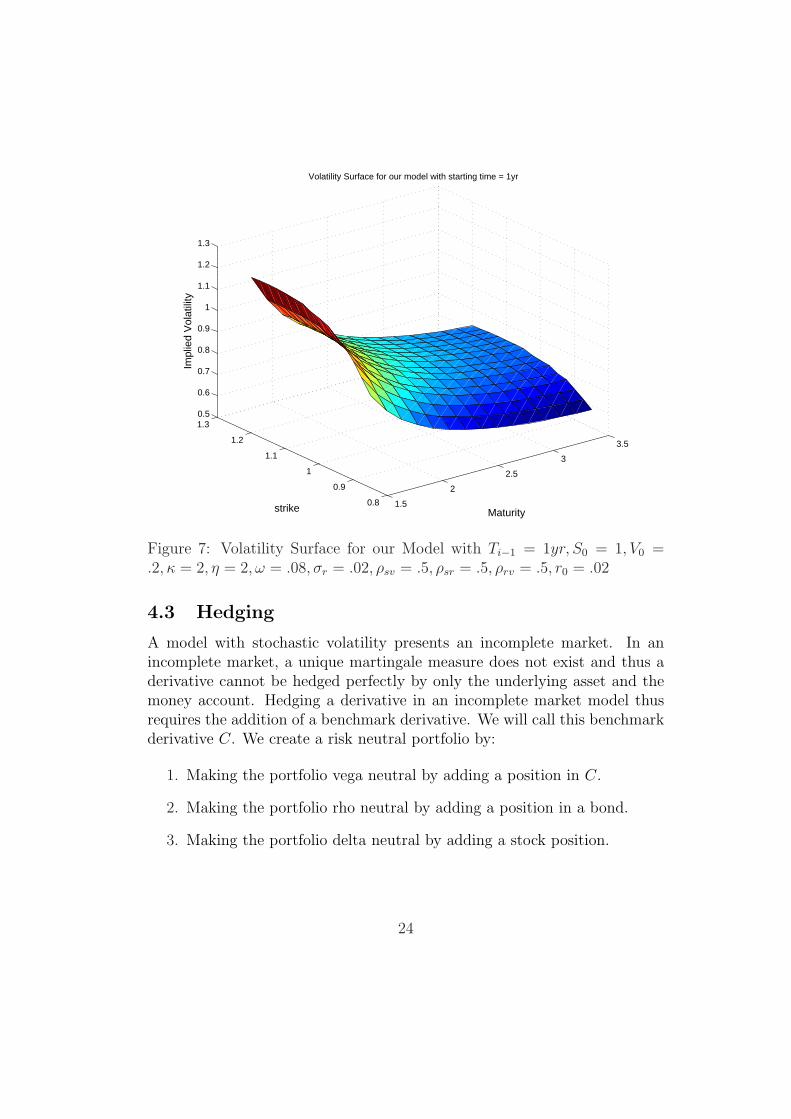
Figure 7: Volatility Surface for our Model with Ti−1 = 1yr, S0 = 1, V0 =.2, κ = 2, η = 2, ω = .08, σr = .02, ρsv = .5, ρsr = .5, ρrv = .5, r0 = .02

4.3 Hedging

A model with stochastic volatility presents an incomplete market. In anincomplete market, a unique martingale measure does not exist and thus aderivative cannot be hedged perfectly by only the underlying asset and themoney account. Hedging a derivative in an incomplete market model thusrequires the addition of a benchmark derivative. We will call this benchmarkderivative C. We create a risk neutral portfolio by:

1. Making the portfolio vega neutral by adding a position in C.

2. Making the portfolio rho neutral by adding a position in a bond.

3. Making the portfolio delta neutral by adding a stock position.

24

5 Hedging Accuracy Tests

In testing the performance of our models, we will evaluate how well the mod-els hedges perform. We highlighted in the stochastic interest rates sectionthat the volatility of the underlying is the only input into the model andthus determines the pricing of the hybrid. For the models to be comparable,we will use the implied volatility from the stochastic volatility and stochasticinterest rate model as the input to get the stochastic interest rate price. Incomparing the prices from the two different models, let Πt0(SISV ) denotethe price from the stochastic volatility and stochastic interest rate model andlet Πt0(SI) denote the price from the stochastic interest rate model.

Πt(SISV ) =P (t0, Ti−1)

{1 + Cfwd(t0, Ti−1, Ti)

}− P (t0, Ti) (85)

Πt0(SI) =P (t0, Ti−1)

{N(d+)−N(d−) + 1

}− P (t0, Ti) (86)

The two prices are similar and will be the same if and only if

N(d+)−N(d−) = Cfwd(t0, Ti−1, Ti) (87)

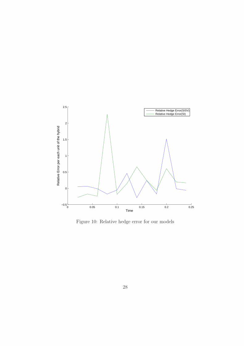
We compare how the hedges perform for a three month period whererebalancing is done weekly. We use Ti−1 = .25 and Ti = .5. We first comparethe two models seperately and then we compare the relative errors of themodels. The data set used for the hedging tests is shown in the appendix.

In comparing the models, we get more information by comparing thestandard errors of the error term. The summation of the squared relativeerrors give us the variance of the error term. Dividing the standard deviationof the errors by the square root of the number of data points used gives usthe standard error. The table below shows the standard errors of the twomodels.

Model Standard ErrorSI 72.56%

SISV 47.74%

We note that the standard error is greater for the stochastic interest ratemodel. This implies that it is better to use the SISV holding all else constant.

25

0 0.05 0.1 0.15 0.2 0.25−2

−1.5

−1

−0.5

0

0.5

1x 10

−3

Time

Val

ue p

er e

ach

unit

of th

e hy

brid

∆ Hedge

∆ Hybrid PriceHedge Error

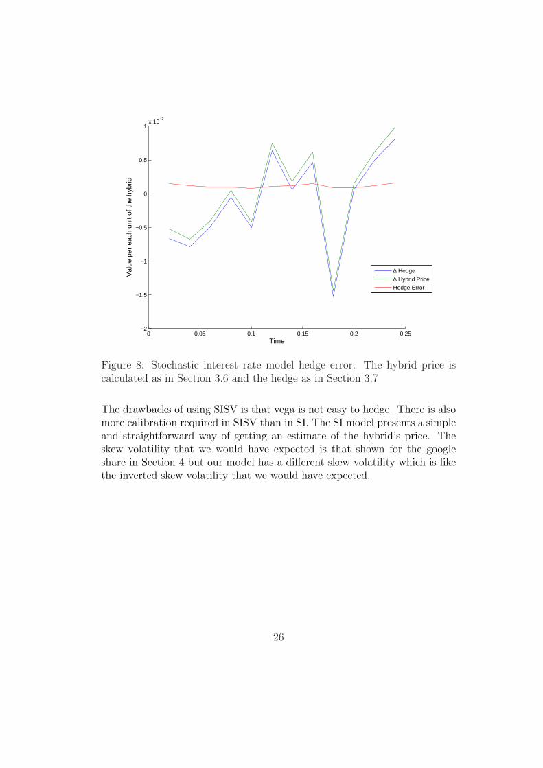
Figure 8: Stochastic interest rate model hedge error. The hybrid price iscalculated as in Section 3.6 and the hedge as in Section 3.7

The drawbacks of using SISV is that vega is not easy to hedge. There is alsomore calibration required in SISV than in SI. The SI model presents a simpleand straightforward way of getting an estimate of the hybrid’s price. Theskew volatility that we would have expected is that shown for the googleshare in Section 4 but our model has a different skew volatility which is likethe inverted skew volatility that we would have expected.

26

0 0.05 0.1 0.15 0.2 0.25−2.5

−2

−1.5

−1

−0.5

0

0.5

1

1.5

2x 10

−3

Time

Val

ue p

er e

ach

unit

of th

e hy

brid

∆ Hedge

∆ Hybrid PriceHedge Error

Figure 9: Stochastic interest rate and stochastic volatility model hedge error.The hybrid price is calculated as in Section 4.2 and the hedge as in Section4.3

27

0 0.05 0.1 0.15 0.2 0.25−0.5

0

0.5

1

1.5

2

2.5

Time

Rel

ativ

e E

rror

per

eac

h un

it of

the

hybr

id

Relative Hedge Error(SISV)Relative Hedge Error(SI)

Figure 10: Relative hedge error for our models

28

0 0.05 0.1 0.15 0.2 0.250

1

2

3

4

5

6

Time

Squ

are

Rel

ativ

e E

rror

per

eac

h un

it of

the

hybr

id

Square of Relative Hedge Error(SI)Square of Relative Hedge Error(SISV)

Figure 11: Square relative hedge error for our models

29

5.1 Conclusion

In this article we have discussed pricing methods for an interest rate hybridproduct. We have priced the hybrid in two ways; using stochastic interestrates alone and also using stochastic interest rates and stochastic volatility.We have found that the pricing of the hybrid is invariant under stochasticinterest rates. We have compared how the models used perform based on howwell they hedge the hybrid. We have found that the stochastic interest ratemodel gives us a simple and straightforward solution but gives us a greatererror than the model with stochastic interest rates and stochastic volatility.We have mentioned that although the stochastic interest rate and stochasticvolatility model is attractive, it is harder to calibrate as well as hedge. Ouranalysis has a shortcoming in that we have priced a forward starting hybridand have only looked at the time before the hybrid has started. Furtherresearch can thus be done to look at the pricing of the hybrid after it hasstarted.

30

6 Data

Time Current Stock Price Current Instantaneous Volatility Current Short Rate0 1 0.2 0.02

0.02 1.115049126 0.200230098 0.0167235630.04 1.06749221 0.2001447 0.0128589470.06 0.599980722 0.19926816 0.0105654380.08 0.492904166 0.198912533 0.0105183250.1 0.506514443 0.198967457 0.0082892880.12 0.59134628 0.199300691 0.0115364840.14 0.877871633 0.200266364 0.012097040.16 0.886192738 0.200285347 0.0145519370.18 0.923664935 0.200370036 0.0080177690.2 0.990715299 0.200515488 0.0084839380.22 1.224401187 0.20098845 0.0108686510.24 0.667152074 0.200073718 0.014616501

31

References

[1] Kristina Andersson. Stochastic Volatility. 2003.

[2] Alexander Batchvarov. Hybrid Products. Risk Books, 2005.

[3] Eric Benhamou and Pierre Gauthier. Impact of Stochastic Interest Ratesand Stochastic Volatility on Variable Annuities. 2009.

[4] Tomas Bjork. Arbitrage Theory in Continuous Time. Oxford UniversityPress, USA, 1999.

[5] Fischer Black and Myron Scholes. The Pricing of Options and CorporateLiabilities. The Journal of Political Economy, 81(3):637–654, 1973.

[6] Peter Carr and Dilip B. Madan. Option Valuation Using the FastFourier Transform. 1999.

[7] Anurag Gupta and Marti G. Subrahmanyam. Pricing and hedging inter-est rate options: Evidence from capfloor markets. European of Bankingand Finance, 29:701–733, 2005.

[8] George Hong. Forward Smile and Derivative Pricing. 2004.

[9] Susanne Kruse. On the Pricing of Forward Starting Options underStochastic Volatility. 2003.

[10] Nimalin Moodley. The Heston Model: A Practical Approach. 2005.

[11] Mikiyo Kii Niizeki. Option Pricing Models: Stochastic Interest Ratesand Volatilities. 1999.

[12] Marcus Overhaus. Equity Hybrid Derivatives. Wiley, 2007.

[13] Rainer Schobel and Jianwei Zhu. Stochastic Volatility With an Orn-steinUhlenbeck Process: Extension. European Finace Review, 3(1):23–46, 1999.

[14] Alexander van Haastrecht. Valuation of long-term hybrid equity-interestrate options. 2008.

32

[15] Alexander van Haastrecht, Roger Lord, Antoon Pelsser, and DavidSchrager. Pricing long-maturity equity and fx derivatives with stochasticinterest rates and stochastic volatility. 2005.

[14, 1, 5, 7, 3, 13, 11, 10, 9, 8, 15, 6, 12, 2, 4]

33