Pricing Interest Rate Derivatives:A General ApproachGeorge ChackoHarvard University
Sanjiv DasSanta Clara University
The relationship between affine stochastic processes and bond pricing equations in expo-nential term structure models has been well established. We connect this result to thepricing of interest rate derivatives. If the term structure model is exponential affine, thenthere is a linkage between the bond pricing solution and the prices of many widelytraded interest rate derivative securities. Our results apply to m-factor processes with ndiffusions and l jump processes. The pricing solutions require at most a single numeri-cal integral, making the model easy to implement. We discuss many options that yieldsolutions using the methods of the article.
The literature on term structure modeling has evolved from one-factor diffu-sion models such as Vasicek (1977) and Cox, Ingersoll, and Ross (1985) tomultifactor models such as Brennan and Schwartz (1977), Duffie and Single-ton (1997), Longstaff and Schwartz (1992), and Balduzzi, Das, and Foresi(1998), as well as jump-diffusion models such as Ahn and Thompson (1988),Bakshi and Madan (2000), Das and Foresi (1996), Das (1998), and Duffie,Pan, and Singleton (2000). The motivation for this evolution in term struc-ture models has come from empirical articles such as Chan et al., Sanders(1992) and Ait-Sahalia (1996).1 However, as work proceeds on better match-ing the dynamics of the short rate to the observed term structure, the areaof fixed income derivative pricing, the main application for modeling theshort rate process, has lagged behind. In this article we attempt to bridgethe gap between the multifactor, jump-diffusion models of the short rate thatare commonly used and the pricing of fixed income derivatives. Specifically
This is a substantially revised version of the article “Pricing Average Interest Rate Options: A GeneralApproach” (1998) based on the original article “Average Interest” (NBER Working Paper no. 6045 [1997]).A substantial part of the work of the second author was done while at Harvard University and the Universityof California, Berkeley. We are indebted for the many helpful comments of the editor and an anonymousreferee who have helped tremendously in improving the content and exposition of the article. Thanks alsoto Marco Avellaneda, Steven Evans, Eric Reiner, Rangarajan Sundaram, Vladimir Finklestein, Alex Levin,Jun Liu, Daniel Stroock, and seminar participants at the Courant Institute of Mathematical Sciences, NewYork University, the Computational Finance Group at Purdue University, University of Texas, Austin, and theRisk99 conference for their comments. Address correspondence to the authors at Harvard University, GraduateSchool of Business Administration, Morgan Hall, Soldiers Field, Boston, MA 02163.
1 Many other articles including those by Brown and Dybvig (1989), Litterman and Scheinkman (1991), andStambaugh (1988) have similar conclusions.
we show that any interest rate process (with any number of factors includingstochastic volatility, stochastic central tendency, etc., or utilizing diffusion orjump-diffusion processes) that leads to an exponential term structure modelalso lends itself to analytic solutions for three large classes of fixed incomesecurities. These methods support numerical techniques which allow for easyimplementation in the context of a no-arbitrage approach. It is our hope thatthe results of this article will allow both researchers and practitioners tofocus on the appropriate stochastic process for the short rate and its factors,and obviate concerns as to whether specific forms of the short rate lead totractable solutions for popular fixed income securities.
The benchmark article of Duffie and Kan (1996) established the linkbetween affine stochastic processes and exponential affine term structuremodels.2 They showed that the factor coefficients of these term structuremodels are solutions to a system of simultaneous Riccati equations and thatthese coefficients are functions of the time to maturity. The kernel of ourtechnique resides in the fact that the solution for different types of inter-est rate options solves an almost identical system of equations. The onlydifference between the two sets of equations is in the constant terms under-lying the equations. By manipulating the Riccati equations and varying theconstant terms, we develop a procedure to price options using the knownsolution components of the original term structure model. Thus we essen-tially show that once the exponential affine term structure model is derived,the pricing formulas for a wide range of popular fixed-income derivatives canbe written by inspection from the components of the term structure model.3
Specifically, we show that this approach is feasible for three large classes offixed income derivatives: those with (1) payoffs that are linear in the shortrate and factors; (2) payoffs that are exponential affine in the short rate andfactors; and (3) payoffs that are an integral over time of a linear combinationof the short rate and factors. These three payoff structures encompass manypopular fixed-income derivatives.
Our technique is general in that it applies to any multifactor, exponentialaffine term structure model with multiple Wiener and jump processes. Nomatter how many jump-diffusion stochastic processes are used, for standardderivatives, our approach involves evaluation of at most two one-dimensionalintegrals, resulting in easy computation. Furthermore, in the final sectionof this article we show that the techniques can be easily extended beyondthe exponential affine class to the class of term structure models we call“exponential separable” models, such as those of Constantinides (1992) andLongstaff (1989). In addition, we also show how to utilize the results of the
2 Dai and Singleton (1997) provide a characterization of the exponential affine class of term structure modelsas they unify and generalize this class.
3 See also Duffie, Pan, and Singleton (2000) and Bakshi and Madan (2000), who developed results that parallelsome of those derived in this article.
196
Pricing Interest Rate Derivatives
article in the context of no-arbitrage models, such as those of Hull and White(1990) and Black, Derman, and Toy (1991), which allow for exact calibrationwith observed data.
To demonstrate the technique we provide closed-form solutions for optionsunder a jump-diffusion model. We price options on bonds, futures, and inter-est rate caps and floors, since these are the most common forms of termstructure derivatives. We also price options on average interest rates, in orderto demonstrate a parsimonious approach based on expansion of the statespace.4 An important tool in our approach is the use of Fourier inversionmethods as in Heston (1993).5. Though the results of this article pertain toterm structure models, the techniques provided extend to several other marketsettings.
The plan of the article is as follows. In Section 1 we specify the interestrate process and the term structure model. We then introduce the pricing tech-nology for fixed income securities that have general payoff functions of theinterest rate process. We proceed in Sections 2–4 to develop analytic solu-tions, in terms of the components of the term structure model in Section 1,for the three categories of derivative payoff functions considered in the arti-cle: linear payoffs in the state variables are handled in Section 2, exponentialaffine payoffs in Section 3, and integro-linear (or a payoff function that isan integral over time of a linear combination of the factors) payoffs aredealt with in Section 4. The details of these derivations are described in theappendix, which contains many analytical features of interest. Section 5 dis-cusses model implementation. Section 6 provides examples of the procedureslaid out in the article. Section 7 presents extensions and Section 8 concludes.
1. Generalized Option Valuation
In this section we present the setup for the general valuation principles inthe article. We specify the general interest rate process and the term structuremodel for which we will be able to derive general option valuation formu-las. The restrictions on the interest rate dynamics imposed here are the sameas those specified in Duffie and Kan (1996) for jump-diffusion processes.These restrictions lead to an exponential affine term structure model. Withthe aid of the Feynman–Kac theorem, which is stated below, we derive a
4 The idea very simply is to expand the state space from that of a traditional Black and Scholes (1973) andMerton (1973) setup with m-state variables to m+1-state variables where the additional variable is the average(i.e., arithmetic integral) of the underlying. Bakshi and Madan (2000) provide a spanning analysis of this idea.
5 Fourier methods have been used subsequently in many articles in finance including Eydeland and Geman(1994), Scott (1995), Bates (1996), Chacko (1996, 1998), Das and Foresi (1996), Bakshi, Cao, and Chen(1997), Bakshi and Madan (1997, 2000), Singleton (1997), and Duffie, Pan, and Singleton (2000), Davydovand Linetsky (1999), Heston and Nandi (1999), Jagannathan and Sun (1999), Leblanc and Scaillet (1998),Levin (1998), Van Steenkiste and Foresi (1999). Bakshi and Madan (1997, 2000) link Fourier transformmethods to a state-price framework, while Duffie, Pan, and Singleton (1998) describe the application of thesetechniques to problems in the area of equity, interest rate and default risk options. Van Steenkiste and Foresi(1999) show how to derive state prices in the same general framework and apply Fast–Fourier methods toprice American options.
197
The Review of Financial Studies / v 15 n 1 2002
general valuation equation for fixed-income securities. Our task in subse-quent sections will be to solve this equation for large classes of fixed-incomesecurities using only the components of the term structure model presentedin this section.
1.1 Interest rate dynamicsThe economy is a continuous-trading economy with a trading interval �0� T �for a fixed T > 0. The uncertainty in the economy is characterized by a prob-ability space �� �Q� which represents the risk-neutral probability measurein the economy.6 Dynamic evolution of the system over time takes place withrespect to a filtration � t� � t ≥ 0� satisfying the conditions in Protter (1990,chap. V).
Let Nt represent a vector l of orthogonal Poisson processes, and let Wt
represent a vector of n Wiener processes. Each Poisson, or jump process, canbe thought of as a counter. When a jump occurs, the jump process incrementsupward by 1 unit. The jump intensities of the Poisson processes are given by�i ≥ 0, i = 1� � � l, and are constant over �0� T �.
The term structure of zero-coupon bond prices is formed from the instan-taneous interest rate and a set of m factors in the economy. The risk-neutralprocesses governing the interest rate and the factors are given by a vector ofstrong Markov processes:
drt = �rv�xv� dt+� ′rv�xv� dW+J′r dN (1)
dxt = �xt� dt+�xt� dW+Jx dN (2)
The m×1 vector, xt , represents a set of Markov factors which influence themarginal productivity of capital, and thus the interest rate, in the economy.We assume that the parameters of the drift, diffusion, and jump coefficients inthe SDE are bounded [in the sense of Gihman and Skorohod (1979, pp. 128–130)], and are such that a unique, strong solution to Equation (1) exists [theconditions in Pardoux (1997) are met] [see also Kurtz and Protter (1996a,b)]. The magnitudes of the Poisson processes are defined by the l×1 vectorJr and the m× l matrix Jx of correlated random variables. It is assumedthat the conditional distribution of the jump size is independent of the statevariables.
We assume that the instantaneous diffusion covariance matrix of the statevariables is given by �xt�, while the vector of instantaneous diffusioncovariances between the state variables xi� t� i = 1� � � m, and rt is given by�xt�.
1.2 Fundamental principlesOur derivations of solutions for the models explored in this article use theFeynman–Kac theorem7 and the Fourier inversion theorem extensively. In
6 Unless indicated otherwise, all computations reported in the article are with respect to the risk-neutral proba-bility measure and not the objective probability measure.
7 See Duffie (1996) for more details regarding the Feynman–Kac relation.
198
Pricing Interest Rate Derivatives
this section we state these for reference and establish the conditions for theirapplicability.
Definition 1. (Feynman–Kac). For any variable X (satisfying the regularityconditions stated below) determined by a stochastic differential equation ofthe form
dXt = �xXt�dt+�xXt�dW + J Xt�dN���the solution, F Xt�, to the expression
Et[e−
∫ Tt gXv�dvf XT �
]�
where f � g ∈�2�1, is determined by the equation
�F Xt�= gXt�F �
where � is the differential operator defined by
�F Xt�=12�2x
&2F
&X2t
+�x&F
&Xt− &F
&'+�Et−�F Xt+ J �−F Xt��(
The boundary condition for this partial differential difference equation isgiven by F XT �= f XT �.
This is simply the univariate version of the differential operator (see note 8for the multivariate version). We will utilize multivariate versions of thistheorem throughout the article. To apply Feynman–Kac, certain regularityconditions must be satisfied by the underlying processes. We require in thisarticle that the processes given in Equations (1) and (2) satisfy these condi-tions, which is stated in univariate form in the following definition.
Definition 2. (Conditions for Feynman–Kac). The process Xt in Remark(1) must satisfy the necessary growth and Lipshitz conditions. [See Duffie(1996, pp. 292–295) or Karatzas and Shreve (1988, p. 366) for explicitdetails. Additional details are available from the exposition in Duffie, Pan,and Singleton (1998).] The conditions required are
1. The functions in question, that is, f � g�����F are continuous.2. The polynomial growth condition is satisfied: �F Xt� t�� ≤ A1 +
Xq�, for some constants A�q > 0.3. f Xt� ≥ 0, or it satisfies a polynomial growth condition in Xt . [Con-
ditions 2 and 3 are either/or type, see Karatzas and Shreve (1988,condition (7.10), p. 366).]
4. For the jump, we will require that the jump transform∫� expcv�dJ v��
c ∈� be well defined.
We also utilize a version of the Fourier inversion formula that relates thecumulative distribution of a density function to its Fourier transform. In thearticle, we regularly solve for the Fourier transform of a density and invertthis transform to get at the cumulative distribution function, which is neededfor security pricing.
199
The Review of Financial Studies / v 15 n 1 2002
Theorem 3. (Fourier Inversion). If the density function f satisfies the fol-lowing conditions [see Shephard (1991)],
1. f is integrable in the Lebesgue sense, that is, f ∈ L.2. Its characteristic function is well defined as -.�= ∫�
−� ei.xf x�dx,
and is integrable [and the characteristic is “well behaved” in thesense defined by Duffie, Pan, and Singleton (1998)].
3. /�-.� exp−i.x�/i.� is uniformly bounded, where /1.� ≡1.�+ 1−.�, then the probability function can be obtained byFourier inversion,
F x�= 12− 1
22
∫ �
0/.
[-.�e−i.x
i.
](
1.3 Bond pricesWith the risk-neutral interest rate process known, we can write an expressionfor the price of any traded security in the economy. Specifically, let Ptr�x4 '�represent the price at time t of a security that matures after a period of time ' .Then, we have the following partial differential difference equation (PDDE)for the price of a bond [Black and Scholes (1973), Merton (1973), Courtadon(1982), Cox, Ingersoll, and Ross (1985), see Ahn and Gao (1999)]:
0 =�Pt+d s′Pt (3)
where d is a row vector of constants and � represents the usual differentialoperator.8 s = �rt�xt�1� is a row vector comprising the current levels of theshort rate and the factors, and an additional parameter required for specialforms of payoff functions.
In the case of traded securities, d = d∗ ≡ �−1�0�0�, but we will assumefor now that d is an arbitrary vector of constants. We do this because insubsequent sections we will utilize transformations to Equation (3) wherepartial differential equations with d �= d∗ will result. For a zero-couponbond that pays off $1 at maturity, the boundary condition that is satisfiedby Equation (3) is P' = 0�= 1.
8 The differential operator applied to a function Pt is defined as
�Pt =12
n∑i=1
�2i rt �xt �
&2Pt&r2
+ 12
m∑i=1
m∑j=1
6ij xt �&2Pt&xi&xj
+m∑i=1
�ixt �&2Pt&r&xi
+�r�xt �&Pt&r
+m∑i=1
�ixt �&Pt&xi
+ &Pt&t
+l∑i=1
�iE�Pr+ Jr�i�xt +Ji�x 4'�−Pr�x4'���
where the expression Ji�x represents a modified version of the matrix Jx of jump magnitudes. Jx is modifiedso that all but the ith column of Jx is zero. This is a direct consequence of Ito’s lemma.
200
Pricing Interest Rate Derivatives
As is well known, we can use the Feynman–Kac theorem to write thesolution to Equation (3) as
P'�= Et[e−
∫ Tt rv dv1
]�
which is the standard discounted form for a discount bond price.We need to impose restrictions on the drift and diffusion terms in Equa-
tions (1) and (2) in order to ensure that the solution to Equation (3) is expo-nential affine. From Duffie and Kan (1996), we know that the term structuresof zero-coupon bond prices are of the exponential affine class, that is, thoseof the form
Pt'�= exp[A'�rt+
m∑i=1
Bi'�xi+C'�]� (4)
where A'��Bi'�� i= 1� � � � �m, and C'� are functions of time to maturityonly if the drift terms and the square of each diffusion term of Equations (1)and (2) are linear in the interest rate and the factors, and if the jump magni-tudes of Equations (1) and (2) have linear (in the interest rate and the factors)moment-generating functions.
The solutions to these functions are each determined by a separate sys-tem of ordinary differential equations (ODEs). Associated with each ODEis a unique boundary condition. For the remainder of the article we willneed to be concerned only with the cases where the boundary conditionsfor Equation (3) are such that resulting boundary conditions on A'�, Bi'��i = 1� � � � �m� and C'� are given by
A0�= a
B10�= b1
((( (5)
Bm0�= bm
C0�= c�
where a�b1� � � � � bm� c are constants. In the case of zero-coupon bond prices,the exponential affine form of these prices allows us to break up Equation (3)using the well-used technique of separation of variables into a set of Ric-cati equations for A'�, Bi'�� i = 1� � � � �m, and C'�. If the boundaryconditions for the system of Riccati equations are given by Equation (5),then the solutions to A'�, B1'�� � � � ,Bm'�, C'� depend on the specificstructure of the drifts, variances, and covariances of the interest rate and thefactors. We denote the solutions to the differential equations governing thesefunctions specifically as A∗;4 '�b�d�, B∗
1;4 '�b�d�� � � � �B∗m;4 '�b�d�,
201
The Review of Financial Studies / v 15 n 1 2002
C∗;4 '�b�d�, respectively, where ; denotes the vector of parameters gov-erning the stochastic processes, and b =�a� b1� � � � � bm� c� denotes the vectorof constants that make up the boundary conditions in Equation (5).
Remark 1. The main result of this article is that the prices of a widerange of common fixed-income derivatives can be characterized solely interms of the functions A∗;4 '�b�d�, B∗
1;4 '�b�d�, � � � , B∗m;4 '�b�d�,
C∗;4 '�b�d�. Therefore we will show that if the interest rate model,regardless of how complicated it is, leads to exponential bond prices, thenthe prices of many interest rate-dependent claims can be easily calculated interms of these functions.
In the case of a discount bond, the holder receives a dollar at maturity,and the boundary condition for the bond can be stated as
PT 0�= 1 = exp[
0rt+m∑i=1
0xi� t+0]( (6)
Therefore the specific boundary conditions for each Riccati equation are allzero, that is, b = 0. Hence the price of the bond is given by
Pt'�=exp[A∗;4'�0�d∗�rt+
m∑i=1
B∗i ;4'�0�d
∗�xi�t+C∗;4'�0�d∗�]( (7)
Virtually all of the term structure models developed in the literature to datebegin with interest rate/factor processes that lead to bond prices of the expo-nential affine form given by Equation (7). Therefore our goal in this articleis to derive pricing implications for derivatives written on this specific classof interest rate processes.
1.4 ExampleWe now present an example of the term structure model discussed in theprevious sections. The example is based on a jump-diffusion model. Thisexample will be continued and extended in subsequent sections of the articlein order to illustrate the use of the theoretical results of the article and,hopefully, to make them more concrete.
Consider the risk-neutral interest process given by the dynamics
dr = <;− r�dt+� dW + Ju dNu�u�− Jd dNd�d�� (8)
where <, ;, � , �u, and �d are constants, while Ju and Jd are exponentiallydistributed random variables with positive means 1u and 1d, respectively. Theinterest rate in this specification displays persistence as well as skewness andexcess kurtosis. The one-jump version of this process was considered in Dasand Foresi (1996). A two-jump model was considered in Duffie, Pan, and
202
Pricing Interest Rate Derivatives
Singleton (2000). The version of Equation (3) that holds for this process isgiven by
12�2Prr +<;− r�Pr −P' +�uE�Pr+ Ju�−Pr��
+�dE�Pr− Jd�−Pr��=−drP�where the subscripts on Pr� denote partial derivatives. The general boundarycondition on Pr� that leads to Equation (5) is given by
Pr� ' = 0�= exp�ar+ c�(Under this boundary condition, the solution to the PDDE is of the form givenby Equation (4):
Pr�= exp�A'�r+C'��� (9)
where A'� and C'� satisfy ordinary differential equations
dA
d'= −<A+d
dC
d'= 1
2�2A2 +<;A+�uE�eAJu −1�+�dE�e−AJd −1�
= 12�2A2 +<;A+�u
(1uA
1−1uA)−�d
(1dA
1+1dA)
with boundary conditions A' = 0� = a and C' = 0� = c. Following theconvention of the previous section, we label the vector �a� c�= b. The solu-tions, labeled A∗'�b�d� and C∗'�b�d�, are given by
A∗'�b�d� = u1e−<' +u2
C∗'�b�d� = u21�
2
4<1− e−2<'�+
[u1u2�
2 +<;u1
<
]1− e−<'�
+[u2
2�2
2+<;u2 −�u−�d
]'
+ �u<−d1u
log
∣∣∣∣ 1−1uu2�e<' −1uu1
1−1uu1 −1uu2
∣∣∣∣+ �d<+d1d
log
∣∣∣∣ 1+1du2�e<' +1du1
1+1du1 +1du2
∣∣∣∣+ cu1 = a−u2
u2 = d
<(
203
The Review of Financial Studies / v 15 n 1 2002
As mentioned in the previous section, in the special case that b= �0�0� andd =−1, the solution to Equation (9) is the price of a zero-coupon bond withmaturity ' . Henceforth throughout the article, we will utilize this example toillustrate the theoretical pricing relationships and numerical methods derivedin the article in the hope of making these results concrete and accessible.To begin, we specify a base set of parameters and price the bond using theequation above. The results are presented in Table 1.
Increasing the upward jump frequency of the short rate causes the bondprice to fall, while the opposite happens as we increase the downward jumpfrequency. Intuitively, as the upward jump frequency increases, the likelihoodof higher future rates increases, and since the bond price is a discountedvalue of these rates, bond prices drop. As both upward and downward jumpfrequency increase, the bond price increases slightly. For example, as bothjump frequencies rise from 3 to 6 jumps per annum, the bond price risesfrom 0.951419 to 0.951424. This is due to the convexity of bond prices withrespect to the short rate. Therefore an equal magnitude upward jump in theshort rate has less effect on bond prices than an equal magnitude downwardjump.
In the following sections we illustrate how to utilize the term structuresolutions to price different options.
1.5 Option pricesIn this section we write a general equation for the pricing of European optionswhere the option payoff may be a general function of the interest rate r . Wedenote the “payoff function” at time T as fT r�x� '�, where r represents thesample path of interest rates and state variables, x, up to time T . In addition,' is a “terminal time period” parameter, which allows the payoff function todepend on a period of time of length ' beyond time T . Therefore the payoffof the option on its expiration date can be expressed as
This table presents bond prices when there are two jumps. The parameters are presented, followed by the prices for varyingjump intensities, �u and �d . The jump intensities for both jumps are set at 5 jumps a year. The jumps are symmetric, in thatthe mean jump size for the positive and negative jumps is 50 basis points. The discount bond price is computed to be 0(9514.We then show bond prices as we vary the jump intensities from 3 to 12 jumps per annum.
204
Pricing Interest Rate Derivatives
where we use the notation Ft'4 '� to represent the price of an option at timet with a period of time ' to expiration written on an underlying security withremaining maturity ' . As a result T = t+ ' . We can use the Feynman–Kacrelation9 to write the price of the option as the discounted expected value ofthe terminal payoff,
Ft'4 '�= Et[e−
∫ Tt rv dv max�fT r�x� '�−K�0�
]� (10)
where the expectation is taken under the risk-neutral measure.10 To simplifynotation, we introduce the variable Zt , defined as
Zt'�=∫ T
trv dv(
We now decompose the price of the option into two expressions as follows:
Ft'4 '� = Et[e−Zt fT r�x� '�1 fT r�x�'�≥K�
]−Et[e−ZtK1 fT r�x�'�≥K�]
= Et[e−Zt fT r�x� '�
]Et
[e−Zt fT r�x� '�1 fT r�x�'�≥K�
Et[e−Zt fT r�x� '�
] ](11)
−KEt�e−Zt �Et[e−Zt1 fT r�x�'�≥K�
Et�e−Zt �
]� (12)
where 1 fT r�x�'�≥K� is an indicator function for when the option finishes up inthe money. However, Et�e
−Zt � is the price of a discount bond that matures attime T ≡ t+ ' . So, Et�e
−Zt �= Pt'� . We define A0�t = Et�e−Zt fT r�x� '��,
which is the present value of the underlying function that determines thepayoff. Now we can rewrite the expression above as
Ft'4 '� = A0� tEt
[e−Zt fT r�x� '�1 fT r�x�'�≥K�
Et�e−Zt fT r�x� '��
]−KPtT �Et
[e−Zt1 fT r�x�'�≥K�
Et�e−Zt �
](
It is clear that Et�e−Zt fT r�x�'�1 fT r�x�'�≥K�
Et �e−Zt fT r�x�'��
� and Et�e−Zt 1 fT r�x�'�≥K�
Et �e−Zt � � are probabili-
ties. For convenience, we denote these two probabilities as A1� t and A2� t ,respectively. The price of the option is restated as
Ft'4 '�=A0�tA1�t−KPt'�A2�t ( (13)
The task at hand is to evaluate A0� t and the two probabilities A1� t andA2� t . The specific equations for A1� t and A2� t may be calculated solely
9 See Duffie (1996) for a exposition of the use of these methods.10 All expectations from this point onward are under the risk-neutral measure unless indicated otherwise.
205
The Review of Financial Studies / v 15 n 1 2002
in terms of the functions A∗;4 '�b�d�, B∗1;4 '�b�d�, � � � , B∗
m;4 '�b�d�,C∗;4 '�b�d� through the application of the Feynman–Kac theorem, whichessentially allows us to solve for any expression of the form in Equation (10)by restating the expression as a solution to a PDDE.
In the next several sections we utilize the Feynman–Kac theorem to tacklethree different types of terminal payoff functions for the pricing of interestrate derivatives:
1. Payoffs that are linear functions of the state variables. These may beused to price caps, floors, yield options, and slope options.
2. Payoffs that are exponential in the state variables, used to price bondoptions, forwards, and futures options.
3. Payoffs that are integrals of the state variables, as in the case of aver-age rate options on the short rate and Asian options on yields.
We now examine each one in turn.
2. Option Pricing for Linear Payoffs
In this section we consider the case when the payoff function is given by alinear function of the interest rate and state variables:
fT r�x� '�= k0rT +k1x1� T +· · ·+kmxm�T +km+1� (14)
where k0� � � � � km+1 are constants. As indicated by Equation (13), the priceof a European call option for this payoff function is given by
Ft'4 '�=A0�tA1�t−KPt'�A2�t ( (15)
We now derive the function A0� t and the two probabilities A1� t and A2� t
for the linear payoff function. Substituting these solutions into Equation (15)will then yield the general option pricing formula for a linear terminal payofffunction.
Proposition 4. (A) The solution for A0� t is given by
A0� t ={B0� t
[&A∗;4 '�b0�d∗�
&Crt+
m∑i=1
&B∗i ;4 '�b0�d∗�
&Cxi�t
+ &C∗;4 '�b0�d∗�&C
]}C=0
206
Pricing Interest Rate Derivatives
where
B0�t = exp[A∗;4 '�b0�d∗�rt+
m∑i=1
B∗i ;4 '�b0�d∗�xi�t+C∗;4 '�b0�d∗�
]
b0 =
Ck0
Ck1(((
CkmCkm+1
(
(B) The characteristic function for A1� t is given by
A1� t =1A0� t
{1iB1� t
[&A∗;4 '�b1�d∗�
&.rt+
m∑i=1
&B∗i ;4 '�b1�d∗�
&.xi�t
+ &C∗;4 '�b1�d∗�&.
]}where
B1�t = exp[A∗;4 '�b1�d∗�rt+
m∑i=1
B∗i ;4 '�b1�d∗�xi�t+C∗;4 '�b1�d∗�
]
b1 =
i.k0
i.k1(((
i.kmi.km+1
(
(C) The characteristic function for A2� t is given by
A2� t =1
Pt'�B1� t (
(D) The characteristic functions in (B) and (C), Ak� t , k = 1�2 , may beinverted to obtain the probabilities Ak�t using a version of Fourier’s theorem(stated earlier):11
Ak�t =12+ 12
∫ �
0Re
(1i.e−i.KAk�t
)d.� k = 1�2
Proof. See the appendix.
We now price specific options that fall into this category of payoffs.
11 Fourier’s inversion theorem for distribution functions can be found in Kendall, Ord, and Stuart (1987) andShephard (1991)
207
The Review of Financial Studies / v 15 n 1 2002
2.1 Interest rate caps and floors, and exoticsAn interest rate cap is an option that pays off when the terminal interestrate exceeds the strike K.12 These options are one of the most widely tradedinstruments in the fixed-income derivatives markets. Many uses are envis-aged. (i) They are routinely used by corporations to cap their funding costs.(ii) Money management companies use floors to ensure a base level of returnin their portfolios. (iii) Caps and floors bear an equivalence to swaps, whichalso makes them useful in managing swaps portfolios. (iv) A collar is a posi-tion containing a long cap and short floor, and one popular version of thesecontracts is a zero-cost collar. For example, investors with a view that interestrates will rise will buy a cap and subsidize themselves by selling a floor.
While the plain vanilla form of the interest-rate cap is now widepsread inusage, more exotic options are being traded, to which the technology of thissection may be put to full use. Examples are as follows: (i) Options on creditspreads are now popular, and the modeling of the term structure of spreadslends itself easily to the pricing of derivatives. (ii) With the introduction ofinflation-indexed bonds, options on inflation may be valued easily, since theterm structure of inflation rates is now becoming available. These optionsmay trade off the TIPS (Treasury inflation-protection securities) market orREALs (an older OTC version of the same security). (iii) An even moreexotic application is one where options on volatility levels may be priced,provided a means of ascertaining volatility is available. Implied volatilitiesare now readily available, and term structures of volatility are also routinelydeveloped, making this an envisageable product. (iv) Finally, these techniquesare also useful for the commodities markets in the pricing of options on con-venience yields. Convenience yields are actively traded, and hedges againstbackwardation and contango risk may be easily set up using options on theterm structure of convenience yields.
A short rate cap may also be viewed as an average rate option where theaveraging period is the last instant before the contract expires. If the capcontract matures at time T , its payoff is given by
CT = rT −K�1rT≥K( (16)
From Equation (16) we have the following pricing result for an interest ratecap:
C0 = EQt �e−ZT rT −K�1rT≥K�( (17)
This option is easily priced using the formula in Proposition 4 by setting theconstants k0 > 0 and k1 = k2 = · · · = km+1 = 0.
12 This is but one possible specification of the cap, making it different from a standard option on a zero couponbond. In another popular market convention, a cap is an option on which the payoff is based on the interest rateat option maturity, but the payment takes place at the end of the period for which the underlying interest rateapplies. We take this up later in this section of Interest, the mathematical treatment for these two conventionsfor caps is quite different.
208
Pricing Interest Rate Derivatives
2.2 Yield caps and floorsWe also consider the case when the cap payoff is made based on yields for anunderlying period. We denote this period �. We price a cap maturing at timeT where the applicable interest rate (denoted R) is based on compoundingover period length �. The payoff at time T +� is given by
�max�0�R−K��which translates into an equivalent payoff at time T of
PrT � T � T +���max�0�R−K�� (18)
where PrT � T � T +�� is the price of the bond with remaining maturity �,denoted as P�� to simplify the notation. Noting that 1+R� = P��−1, wehave
R=(
1P��
−1)
1�(
Using Equation (18) we may write the value of the cap at time 0 as follows:
capt=0 = �E0�e−ZT max 0� P��R−P��K��
= �E0
[e−ZT max
{0� P��
(1
P��−1
)1�−P��K
}]= E0
[e−ZT max 0�1−P��−�P��K�]
= E0�e−ZT max 0�1−P��1+�K���
= 1+�K�E0
[e−ZT max
{0�
11+�K −P��
}]�
which is straightforward to value since the expression above embeds theformula for a put option of maturity T , on a zero-coupon bond of maturityT +��, with a strike price of 1/1+�K�. The formula for these options isdeveloped in the following sections.
Yield options may be priced more generally by choosing the weightsappropriately in the linear payoff function to match the coefficientsof the yield equation. In order to price a cap on �-maturity yield,Proposition 4 applies with k0 = A∗;4��0�d∗�, k1 = B∗
1;4��0�d∗�, � � � ,km = B∗
m;4��0�d∗�, km+1 = C∗;4��0�d∗�, and recall that d∗ = �−1�0�0�.This version of the model may be used for caps and floors on Libor yields.
2.3 Yield combo optionsA “combo” option is one where the payoff depends on a basket of yields,weighted in any chosen proportions. If the payoff is determined based on nyields with weights xi� i = 1((n and maturities �i� i = 1((n, then the option
209
The Review of Financial Studies / v 15 n 1 2002
is priced using the result in Proposition 4 with the constants set as fol-lows: k0 = ∑n
i=1 xiA∗;4�i�0�d∗�, k1 = ∑n
i=1 xiB∗1;4�i�0�d∗�, � � � , km =∑n
i=1 xiB∗m;4�i�0�d∗�, km+1 =
∑ni=1 xiC
∗;4�i�0�d∗�.There are many types of combo options in the market. (i) A special case
of combo options are yield curve “slope” options, based on the differenceof two yields [see Duffie, Pan, and Singleton (2000)]. (ii) Differences inthe levels of term structures in different markets may be exploited in thesemodels. For example, “diff swaps” have been in place for quite a while—yield combo options are another way to achieve the benefits of diff swapsusing packages of options. These “basis rate” transactions are gaining inpopularity as markets across the world develop much tighter interactions andlinkages. (iii) In the foreign currency markets, we have “currency couponswaps” which are options on two different LIBOR rates. These transactionshave become popular with the onset of the European Monetary System. (iv)“Basket” yield options allow trading on a basket of different interest rates,usually reducing corporation hedging costs.13
2.4 ExampleUnder the parameters of the two-jump example of the previous section, weprice a cap on the short rate, at an exercise level of 10%. Using the equationsfrom Proposition 4, we present the formula as:(A) The solution for A0� t is given by (b0 = �C�0��d∗ = �−1�0�)
A0� t ={B0� t
[&A∗;4 '�b0�d∗�
&Crt+
&C∗;4 '�b0�d∗�&C
]}C=0
B0� t = exp�A∗;4 '�b0�d∗�rt+C∗;4 '�b0�d∗��(
(B) The characteristic function for A1� t is given by (b1 = �i.�0�)
A1� t =1A0� t
{1iB1� t
[&A∗;4 '�b1�d∗�
&.rt+
&C∗;4 '�b1�d∗�&.
]}B1� t = exp�A∗;4 '�b1�d∗�rt+C∗;4 '�b1�d∗��(
(C) The characteristic function for A2� t is given by
A2� t =1
Pt'�B1� t (
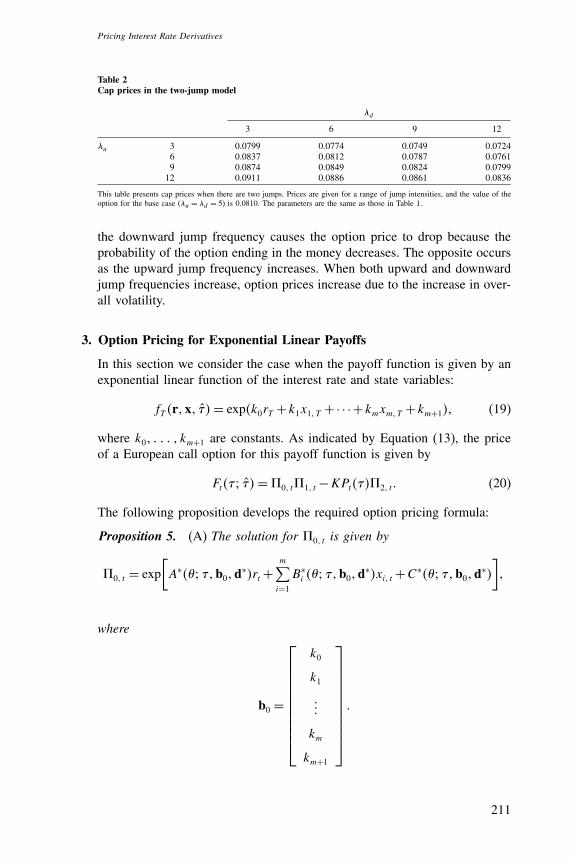
For illustration, we compute prices for caps given a range of jump inten-sities, and the results are summarized in Table 2. The value of the option forthe base case (�u = �d = 5) is 0(0810. As one would expect, an increase in
13 It is fortuitous that so many options may be priced as linear combinations of yields. The simplicity of thesetechniques is obviated, however, when nonlinear combinations of yields need to be considered or for nonlinearcombinations of bond prices.
This table presents cap prices when there are two jumps. Prices are given for a range of jump intensities, and the value of theoption for the base case (�u = �d = 5) is 0(0810. The parameters are the same as those in Table 1.
the downward jump frequency causes the option price to drop because theprobability of the option ending in the money decreases. The opposite occursas the upward jump frequency increases. When both upward and downwardjump frequencies increase, option prices increase due to the increase in over-all volatility.
3. Option Pricing for Exponential Linear Payoffs
In this section we consider the case when the payoff function is given by anexponential linear function of the interest rate and state variables:
fT r�x� '�= expk0rT +k1x1� T +· · ·+kmxm�T +km+1�� (19)
where k0� � � � � km+1 are constants. As indicated by Equation (13), the priceof a European call option for this payoff function is given by
Ft'4 '�=A0� tA1� t−KPt'�A2� t ( (20)
The following proposition develops the required option pricing formula:
Proposition 5. (A) The solution for A0� t is given by
A0� t = exp[A∗;4 '�b0�d∗�rt+
m∑i=1
B∗i ;4 '�b0�d∗�xi� t+C∗;4 '�b0�d∗�
]�
where
b0 =
k0
k1
(((
km
km+1
(
211
The Review of Financial Studies / v 15 n 1 2002
(B) The characteristic function for A1� t is given by
A1� t =1A0� t
exp[A∗;4 '�b1�d∗�rt+
m∑i=1
B∗i ;4 '�b1�d∗�xi�t
+C∗;4 '�b1�d∗�]� (21)
where
b1 =
1+ i.�k0
1+ i.�k1
(((
1+ i.�km
(
(C) The characteristic function for A2� t is given by
A2� t =1
Pt'�exp
[A∗;4 '�b2�d∗�rt+
m∑i=1
B∗i ;4 '�b2�d∗�xi�t
+C∗;4 '�b2�d∗�]� (22)
where
b2 =
i.k0
i.k1
(((
i.km
(
(D) We invert Ak� t to obtain the probability Ak�t using a version of Fourier’stheorem:
Ak�t =12+ 12
∫ �
0Re
(1i.e−i.KAk� t
)d.� k = 1�2(
Proof. See the appendix.
The following three sections consider specific cases of this class of payofffunction.
212
Pricing Interest Rate Derivatives
3.1 Discount bond optionsBond options have been traded since the late 1970s and are the oldest formof interest rate option contract.14 A European call option on a discount bondat strike K is the right but not the obligation to purchase a discount bondwith remaining maturity ' on the expiration date of the option. The optionpayoff is
FT 04 '�= max�PT '�−K�0�(
The price of the bond option is the discounted expected value of the terminalpayoff:
Ft'4 '� = Et[e−
∫ Tt rvdv max�PT '�−K�0�
]= Et
[e−Zt'�PT '�
]A1� t−KPt'�A2�t
= Pt'+ '�A1� t−KPt'�A2� t ( (23)
This is easily priced, an examination of the results of Proposition 5 revealsthat setting the constants to the following values provides the value ofthe bond option: k0 = A∗;4��0�d∗�, k1 = B∗
1;4��0�d∗�� � � � , km = B∗m
;4��0�d∗�, km+1 = C∗;4��0�d∗�.
3.2 Futures and forwards on discount bondsWe begin with a derivation of forward and futures prices. Let Fd� t'4 '�denote the '-period-ahead forward price of a '-period bond at time t. Bydefinition, the forward price is simply the ratio of the ' + '�-period bondprice over the '-period bond price:
Fd� t'4 '�=Pt'+ '�Pt'�
( (24)
Let Fu� t'4 '� denote the '-period-ahead futures price of a '-period bond attime t. The futures price is given by a simple application of the exponentialmodel:
Fu� t'4 '� = exp[A∗;4 t+ '�b�d�rt+
m∑i=1
B∗i ;4 t+ '�b�d�xi� t
+C∗;4 t+ '�b�d�]� (25)
14 Pricing formulas for bond options were available as early as that of the Vasicek (1977) model and the Cox,Ingersoll, and Ross (1985) model. Since then, many other articles have dealt with bond option models:Courtadon (1982), Ho and Lee (1986), Jamshidian (1989), Carverhill and Clewlow (1990), Shirakawa (1991),Heath, Jarrow, and Morton (1992), Longstaff and Schwartz (1992), Geman and Yor (1993), Heston (1993),Naik and Lee (1993), Yor (1993), Eydeland and Geman (1994), Das and Foresi (1996), Das (1997), Duffie,Pan, and Singleton (2000), Leblanc and Scaillet (1998), and Heston and Nandi (1999).
213
The Review of Financial Studies / v 15 n 1 2002
where
b =
A∗;4 t+ '�0�d∗�
B∗1;4 t+ '�0�d∗�
(((
B∗m;4 t+ '�0�d∗�
C∗;4 t+ '�0�d∗�
d = �0�0�0�(
Note here that d �= d∗ as in the previous subsection.
3.3 Discount bond futures optionsFutures options are traded on exchanges and are typically liquid contracts. AEuropean call option on a discount bond future at strike K is the right butnot the obligation to purchase a bond future with remaining maturity ' onthe expiration date of the option. Let Ft'4 '� '
′� be the price of an optionwith time-to-expiration ' , written on a futures contract with time to maturity' that calls for the delivery of a discount bond with time to maturity ' ′. Theoption payoff is
FT 04 '� '′�= max�Fu�T '4 '
′�−K�0�(
The futures option is easily priced using the results of Proposition 5. Settingthe constants to the following values provides the value of the bond option:k0 = A∗;4��0�d�, k1 = B∗
1;4��0�d�� � � � , km = B∗m;4��0�d�, km+1 =
C∗;4��0�d�, where d = �0�0�0�. A common type of contract to whichthese techniques apply are Euro-currency futures options.
3.4 ExampleAs an example of the models in this section, we price bond options ondiscount bonds of half-year remaining maturity ' = 0(5�, where the optionmaturity is also a half year ' = 0(5�. The representative equations fromProposition 5 are as follows:
(A) The solution forA0� t is given by (b0 = �A∗;4 '�b0�d∗��C∗;4 '�b0�d∗��,d∗ = �−1�0�)
A0� t = exp�A∗;4 '�b0�d∗�rt+C∗;4 '�b0�d∗��(
(B) The characteristic function for A1� t is given by
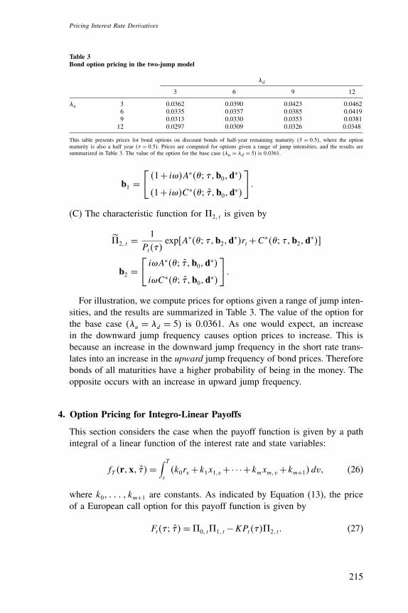
This table presents prices for bond options on discount bonds of half-year remaining maturity ' = 0(5�, where the optionmaturity is also a half year ' = 0(5�. Prices are computed for options given a range of jump intensities, and the results aresummarized in Table 3. The value of the option for the base case (�u = �d = 5) is 0(0361.
b1 =[1+ i.�A∗;4 '�b0�d∗�
1+ i.�C∗;4 '�b0�d∗�
](
(C) The characteristic function for A2� t is given by
A2� t =1
Pt'�exp�A∗;4 '�b2�d∗�rt+C∗;4 '�b2�d∗��
b2 =[i.A∗;4 '�b0�d∗�
i.C∗;4 '�b0�d∗�
](
For illustration, we compute prices for options given a range of jump inten-sities, and the results are summarized in Table 3. The value of the option forthe base case (�u = �d = 5) is 0(0361. As one would expect, an increasein the downward jump frequency causes option prices to increase. This isbecause an increase in the downward jump frequency in the short rate trans-lates into an increase in the upward jump frequency of bond prices. Thereforebonds of all maturities have a higher probability of being in the money. Theopposite occurs with an increase in upward jump frequency.
4. Option Pricing for Integro-Linear Payoffs
This section considers the case when the payoff function is given by a pathintegral of a linear function of the interest rate and state variables:
fT r�x� '�=∫ T
tk0rv+k1x1�v+· · ·+kmxm�v+km+1�dv� (26)
where k0� � � � � km+1 are constants. As indicated by Equation (13), the priceof a European call option for this payoff function is given by
Ft'4 '�=A0� tA1� t−KPt'�A2� t ( (27)
215
The Review of Financial Studies / v 15 n 1 2002
Proposition 6. (A) The solution for A0� t is given by
A0� t ={Et×
[&A∗;4 '�0�d0�
&Crt+
m∑i=1
&B∗i ;4 '�0�d0�
&Cxi�t
+ &C∗;4 '�0�d0�
&C
]}C=0
�
where
Et = exp[A∗;4 '�0�d0�rt+
m∑i=1
B∗i ;4 '�0�d0�xi�t+C∗;4 '�0�d0�
]
d′0 =
Ck0 −1
Ck1
(((
Ckm
Ckm+1
(
(B) The characteristic function for A1� t is given by
A1� t =1A0� t
{Et×
[&A∗;4 '�0�d0�
&Crt+
m∑i=1
&B∗i ;4 '�0�d0�
&Cxi� t
+ &C∗;4 '�0�d0�
&C
]}C=i.
(
(C) The characteristic function for A2� t is given by
A2� t =1
Pt'�exp
[A∗;4 '�0�d0�rt+
m∑i=1
B∗i ;4 '�0�d0�xi� t
+C∗;4 '�0�d0�
]C=i.
(
(D) We invert Ak� t to obtain the probability Ak�t using a version of Fourier’stheorem:
Ak�t =12+ 12
∫ �
0Re
(1i.e−i.KAk� t
)d.� k = 1�2(
Proof. See the appendix.
This payoff class relates to the pricing of average (Asian) options on shortrates and yields.
216
Pricing Interest Rate Derivatives
4.1 Asian optionsAsian options15 have several uses: (i) Banks and corporations use them tohedge their financing costs over an extended period of time rather than relyon more traditional contracts such as caps, floors, and collars. (ii) Corpora-tions that have cash flows over a period of time may use an Asian optioninstead of a series of conventional options to hedge the risks associated withthese cash flows. Asian options are often cheaper than regular options, whichmakes hedging cost effective. (iii) The writers of caps and floors may useAsian options to hedge their risk on these contracts over several maturities.(iv) Interest differentials are known to follow mean-reverting processes, andAsian options written on the average interest differential of two currenciesmay be used to hedge risk in a portfolio of long-term foreign currency optionsover a range of maturities. (v) Binary Asian options may be used to cover“event risk”, such contracts pay off a fixed amount only if an event occurs.An example of such contracts is one where two parties contract on whethermarket convergence between two interest rates will occur or not. In this set-ting, the rationale for the binary Asian option lies in the fact that interest rateswill be in one of two regimes (high or low) depending on the outcome ofconvergence. Since regimes are often difficult to detect empirically, writingoptions on the average of a financial variable over a period of time is morelikely to ensure that a financial variable actually resides within a regime thanwhen a variable is examined only at one point in time. (vi) Asian options areless susceptible to market manipulation by the option’s counterparties, sinceit is harder to manipulate a market over an extended period of time. (vii)And finally, Fed funds futures and options are contingent on the average Fedfunds rate during a month.16
Proposition 6 provides the pricing of Asian options on the short rate andyields. This complements the work of Longstaff (1995), who has developeda similar single-factor model using different methods. Geman and Yor (1993)use Bessel process methods to value perpetuities in both the O-U and square-root process models.17 In this article, alternative methods for finite timeintegrals of mean-reverting Brownian motions are developed by means ofstate-space expansion.18
15 In the literature on Asian options, various analytical solutions have been obtained. Geman and Yor (1993)provide a solution for the arithmetic average option when the underlying follows a Bessel process. Mostof the work done on techniques for pricing Asian options focuses on numerical techniques such as MonteCarlo simulation or lattice-based methods. Examples of interesting numerical techniques for the Asian optionproblem with geometric Brownian motions include Yor (1993), De-Schepper, Teunen, and Goovaerts (1994),and Dewynne and Wilmott (1995) Barraquand and Pudet (1996). In addition, the overwhelming majority ofwork has focused on Asian options written on a stock price or a foreign exchange rate, where the use ofgeometric Brownian motion may be deemed appropriate.
16 We are grateful to the referee for suggestions of possible contracts that may be priced using these techniques.17 Perpetuities are also integrals of exponentials of a Brownian motion and hence are logically subsumed within
the framework of Geman and Yor (1993). This issue also connects with the work on perpetuities by Dufresne(1990). See also Bouaziz, Briys, and Crouhy (1994).
18 In an earlier version of the article, our method for binary Asian options on jump diffusion processes hadnot been extended to standard Asian options, developed originally by Bakshi and Madan (1997, 2000),
217
The Review of Financial Studies / v 15 n 1 2002
Asian options on the short rate are priced using a special case of Proposition 6where k0 > 0� k1 = k2 = · · · = km+1. However, Asian options on yields are farmore widely used, such as in the case of options on the average of the 3-or6-month yield. These are also amenable to Proposition 6 with k0 = A∗;4�,0�d∗�� k1 =B∗
where the option is written on the average of the �-maturity yield.
4.2 ExampleAs an example, we extend the two-jump model to the pricing of an Asian optionon the short rate. The option maturity is a half year ' = 0(5� and the exerciselevel of the average rate is 10%. The equations from Proposition 6 are(A) The solution forA0� t is given by
A0� t ={Et×
[&A∗;4 '�0�d0�
&Crt+
&C∗;4 '�0�d0�
&C
]}C=0
Et = exp�A∗;4 '�0�d0�rt+C∗;4 '�0�d0��
d′0 =
[C−1
0
](
(B) The characteristic function forA1� t is given by
A1� t =1A0� t
{Et×
[&A∗;4 '�0�d0�
&Crt+
&C∗;4 '�0�d0�
&C
]}C=i.
(
(C) The characteristic function forA2� t is given by
A2� t =1
Pt'�exp�A∗;4 '�0�d0�rt+C∗;4 '�0�d0��C=i.(
While the jump example is merely illustrative, numerical examples for theAsian option model and other models are provided in Section 6.
5. Model Implementation
Thesolutionsprovided in theprevious sectionsprovideaconvenient setof resultsthat should allow researchers to write down pricing solutions to exponential termstructure models in one quick step. However, the implementation of these modelsfor actual pricing purposes requires calibration of the base term structure modelagainst a set of data. In this section we extend the approach in Duffie and Kan(1996) to show how calibration can readily be accomplished, and subsequentlywe show how to implement option pricing using the calibrated model.
for diffusion processes. Here we provide complete solutions to all Asian-type contracts in the particularframework of this article, which complements the results of Bakshi and Madan, and more recently, for jumpdiffusions, by Duffie, Pan, and Singleton (2000).
218
Pricing Interest Rate Derivatives
Calibration of the model using a cross-section of bond prices provides one wayof obtaining the risk-neutral parameters required for derivative security pricing.In the class of models investigated in this article, it is possible to obtain parameterestimates directly off the Riccati equations for the term structure model. We callthis approach “pricing by estimation of primitives.”
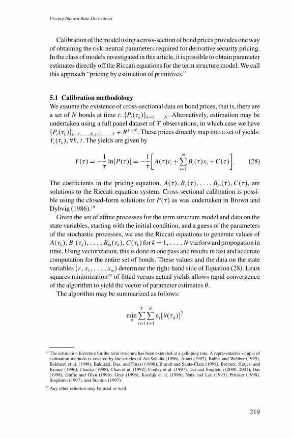
5.1 Calibration methodologyWe assume the existence of cross-sectional data on bond prices, that is, there area set of N bonds at time t� Pt'k��k=1� � � � �N . Alternatively, estimation may beundertaken using a full panel dataset of T observations, in which case we have Pt'k��k=1� � � � �N �t=1� � � � �T ∈ RT×N . These prices directly map into a set of yields:Yt'k��∀k� t. The yields are given by
Y '�=−1'
ln�P'��=−1'
[A'�rt+
m∑i=1
Bi'�xi+C'�]( (28)
The coefficients in the pricing equation, A'��B1'�� � � � �Bm'��C'�, aresolutions to the Riccati equation system. Cross-sectional calibration is possi-ble using the closed-form solutions for P'� as was undertaken in Brown andDybvig (1986).19
Given the set of affine processes for the term structure model and data on thestate variables, starting with the initial condition, and a guess of the parametersof the stochastic processes, we use the Riccati equations to generate values ofA'k��B1'k�� � � � �Bm'k��C'k� fork= 1� � � � �N via forward propogation intime. Using vectorization, this is done in one pass and results in fast and accuratecomputation for the entire set of bonds. These values and the data on the statevariables r� x1� � � � � xm� determine the right-hand side of Equation (28). Leastsquares minimization20 of fitted versus actual yields allows rapid convergenceof the algorithm to yield the vector of parameter estimates ;.
The algorithm may be summarized as follows:
min;
T∑t=1
N∑k=1
Gt�;'k��2
19 The estimation literature for the term structure has been extended at a galloping rate. A representative sample ofestimation methods is covered by the articles of Ait-Sahalia (1996), Attari (1997), Babbs and Webber (1995),Balduzzi et al. (1998), Balduzzi, Das, and Foresi (1998), Brandt and Santa-Clara (1998), Brenner, Harjes, andKroner (1996), Chacko (1998), Chan et al. (1992), Conley et al. (1997), Dai and Singleton (2000, 2001), Das(1998), Duffie and Glyn (1996), Gray (1996), Koedijk et al. (1996), Naik and Lee (1993), Pritsker (1998),Singleton (1997), and Stanton (1997).
20 Any other criterion may be used as well.
219
The Review of Financial Studies / v 15 n 1 2002
subject to
Gt�;'k��=Y 'k�+1'
[A'k�rt+
m∑i=1
Bi'k�xit+C'k�]
&A
&'= 1
2
n∑i=1
�2r� iA
2 +�rA+d� ∀'k�d =−1�A0�= 0
&B1
&'= 1
2
m∑i=1
n∑j=1
62x1� ij
BiBj +m∑i=1
�x1� iABi+
n∑i=1
�2x1� iA2
+�x1A+
m∑i=1
�x1� iBi� ∀'k� �B10�� � � � �Bm0��
′ = 0
(((
&Bm&'
= 12
m∑i=1
n∑j=1
6xm� ijBiBj +
m∑i=1
�xm� iABi+n∑i=1
�2xm� iA2
+�xmA+m∑i=1
�xm� iBi ∀'k� �B10�� � � � �Bm0��′ = 0
&C
&'= 1
2
n∑j=1
�jA2 +�A+ 1
2
m∑i=1
n∑j=1
6ijBiBj
+m∑i=1
�iBi+m∑i=1
�iABi+l∑i=1
�i
× (E[eAJr� i+B1Jx�1i+···+BmJx�mi]−1
) ∀'k�C0�= 0(
(29)
This approach has many useful features. First, since the Riccati equation sys-tem [Equation (29)] consists entirely of first-order ordinary differential equa-tions, generation of the value set A'k��B1'k�� � � � �Bm'k��C'k� for a given; is very accurate.21 Second, since the calibration equation is linear, and theobjective function is quadratic, we obtain a well-behaved optimization problem.Third, we retain thechoiceofundertakingcalibrationeither for theentirepanelofdata or for a single cross-section only. Fourth, since the information used relatesdirectly to the prices of derivative securities, all estimated parameters are withrespect to the risk-neutral measure and may be used for pricing immediately.22
21 Indeed, standard mathematical packages yield highly accurate results. We found the ode45 function in Matlabto be extremely fast and accurate. This is but one example of the power of using the original Riccati equations.Other facile implementations using characteristic function estimators are considered in Chacko (1998) andSingleton (1997).
22 Appendix B gives an example of the implementation for the Vasicek (1997) model. Extending the estimationprocedure to calibration off option prices involves only one extra dimension in the ODE generator for theparameter .. See the following section.
220
Pricing Interest Rate Derivatives
5.2 The implementation of option pricingAs an example, we consider the pricing of bond options for which the equationis Ft'4 '�= Pt'+ '�A1� t−KPt'�A2� t , whereK is the strike price. There arefour components to this model: (i) an underlying bond of maturity ' + '�, (ii)a bond of the same maturity (') as the option, (iii) the probability of the optionfinishing in the money (A2� t), and (iv) the present value of a dollar conditionalon the option finishing in the money (A1� t). Since the first two components aredirectly observable from the market, we need only compute the two probabilityvalues.
Since A2� t is not directly computable, we obtain its characteristic func-tion, A2� t , which is the solution to the Riccati differential equation system[Equation (29)]. We propogate the differential equation system forward totime T , beginning with the appropriate initial conditions, which are (seeProposition 5)
b =
i.A∗;4 '�0�d∗�
i.B∗1;4 '�0�d∗�
(((
i.B∗m;4 '�0�d∗�
i.C∗;4 '�0�d∗�
( (30)
The valuesA∗;4'�0�d∗��B∗1;4'�0�d∗�� � � � �B∗
m;4 '�0�d∗��C∗;4'�0�d∗�are the coefficients from boundary conditions that have been computed from thecalibration step and are therefore already available. Hence the vector b is com-pletelyknown,and formsanobservable initial condition for forwardpropogationvia the Riccati system. For implementation purposes we discretize the state spaceon which the Fourier inversion parameter. resides, that is, generate a finite sup-port set. ∈ 0�.1�.2� � � � � .�with equal intervals/.. This generates via theRiccati system a set of values of the probability A2� t.� for each value of ..Fourier inversion yields the probabilitiesA1� t andA2� t .
23
6. Illustrative Examples
In this section we present examples illustrating the techniques of the article. Thepurpose of the section is not to develop pricing solutions for new models but
23 Since the Fourier inversion involves a complex integral from zero to infinity, it is often numerically unstable. Oneapproach is to simply use an integration package such as that available from Mathematica. Otherwise a suitablediscretization also leads to fairly accurate results. Since the upper limit of the integral is infinity, any numericalscheme that truncates the integral needs to check carefully that the tail of the integral has died out before thetruncation point. For a similar discussion, see also the use of Fourier inversion via integration in estimationtechnology developed in Singleton (1997). Singleton provides an extensive discussion of the appropriate choiceof discrete grid for the implementation of the procedure.
221
The Review of Financial Studies / v 15 n 1 2002
instead is to illustrate how to use the techniques developed in earlier sections ofthis article. This is best done in the context of simple models. We analyze exoticoptions such as range-Asians and credit spread calls, and we provide results for aversion of the jump diffusion example that has been used throughout this article.
6.1 Range-Asian optionsWe explore a more exotic option, the range-Asian. The process on which thisoption is written is the simple Vasicek model, that is, Equation (8) devoid of thejump component. The range-Asian is an interesting option to analyze because itoffers a good setting in which the joint effects of the mean rate, ;, and the rateof mean reversion, k, may be examined. In general, a range option is one thatpays off a certain amount each day if the value of the underlying variable lieswithin a pre specified range. The range-Asian pays off each day that the currentaverage up to that date remains within prespecified limits. These options havedaily payoffs that are based on whether the average interest rate up to time t lieswithin a prespecified range �at�� bt��� at� < bt�� ∀t ∈ �0� T �. In the articlewe assume that at� = a and bt� = b, without loss of generality. The value ofthese options is simply
R�at�� bt�� T � = 1
d
d∑j=1
�Qat�� t�−Qbt�� t��
d = FlrT ∗365�
t = j
365�
where Q(� is the value of a binary Asian option, and Flrx� is a function thatreturns the greatest integer less than or equal toK. Our analyses utilize both thesquare-root and the O-U process models.
Pricing examples for range-Asian options are presented in Table 4. Theseprices increasewhentherangewidens.Whenthemeanrate; lies inside therange,increases in mean reversion (k) drive the price upward. This is because, ask rises,the likelihood of the interest rate remaining within the range increases, therebyraising value. When the mean lies outside the range, option prices decrease whenk increases because the interest rate is less likely to remain in the desired range.This is true of both cases, when the mean is above and below the range, that is,; = 0(15 and ; = 0(05, respectively.
6.2 The jump diffusion modelIn this section we analyze the pricing of Asian options in a jump diffusion frame-work. In particular, we extend the results of Das and Foresi (1996) to the pricingof Asian options on jump diffusions. The underlying interest rate process is asfollows:
dr = k;− r�dt+� dz+ J J���dQ��(
222
Pricing Interest Rate Derivatives
Table 4Pricing range-Asian options
Range k = 0(5 k = 1(5 k = 2(5
; = 0(05a= 0(09� b = 0(11 0.3718 0.3539 0.3075a= 0(08� b = 0(12 0.6631 0.6461 0.5923a= 0(07� b = 0(13 0.8388 0.8353 0.8066
; = 0(10
a= 0(09� b = 0(11 0.3818 0.4120 0.4424a= 0(08� b = 0(12 0.6741 0.7132 0.7488a= 0(07� b = 0(13 0.8435 0.8714 0.8922
; = 0(15
a= 0(09� b = 0(11 0.3823 0.3810 0.3406a= 0(08� b = 0(12 0.6717 0.6646 0.6150a= 0(07� b = 0(13 0.8374 0.8265 0.7938
The following table presents the values of the range-Asian option. This option is written over a fixed number of days. Everyday the option pays off if the average interest rate up to that day lies within a range a� b�. The payoff is a dollar divided bythe number of days the option is written for. The values in this table are for a range-Asian option with maturity T = 0(2 years,that is, 73 days. The parameters that are varied are (a) mean reversion ( k), (b) lower range limit (a), and (c) upper range limit(b). The base parameters used are initial interest rate (r0 = 0(1), time to maturity (T = 0(2), mean rate (; = 0(1), market priceof risk (K = 0), volatility (1 = 0(2).
Here, k is the rate of mean reversion, ; is the long-run mean of the interest rate,� is the coefficient of diffusion volatility, and dz is the Wiener increment. Thejump portion has a point process Q with jump arrival intensity � and the jumpJ has a sign determined by parameter J, which represents the probability of apositive jump. The parameter� > 0 defines the jump size and is the distributionparameter for an exponential distribution, such that it has mean 1
�, that is, the
probability density function is given by f J �= �e−�J . As an example, we pricebonds and options with the following base case parameters:
k ; � � � J r '
2 0.1 0.02 5 50 1 0.1 3
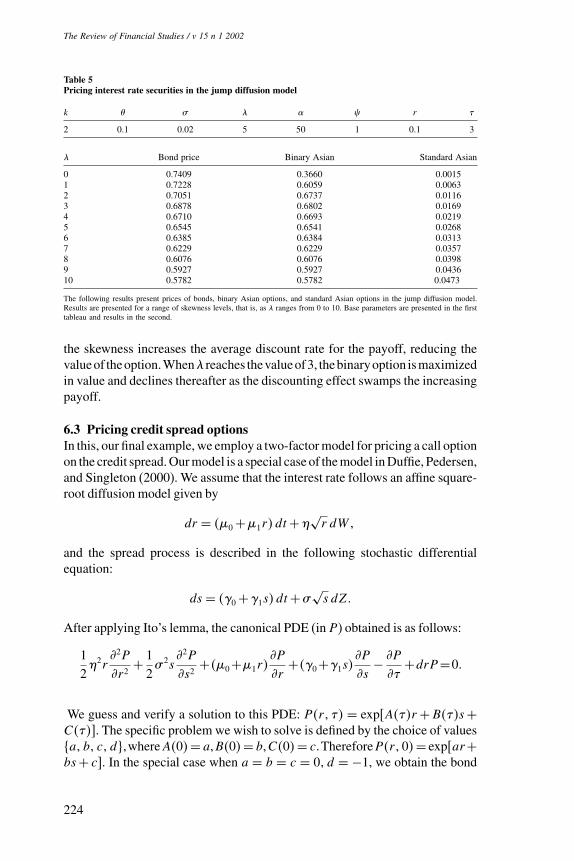
Bondmaturity isdenoted' .This results inadiscountbondpriceofP0(1�3�=0(6545. As an illustration we choose one interesting case, that is, J = 1, whichindicates that there will only be positive jumps, and this diminishes the proba-bility of negative interest rates, but also injects a substantial quantity of positiveskewness in interest rates. We shall vary the jump intensity �� from 0 to 10 tosee how increasing skewness affects the price of the binary Asian option and thestandard Asian option.
Pricing results are presented in Table 5. The standard Asian option of coursehas lower values, and since it is probability weighted, the payoff effect is alwaysstrong enough to outweigh the discounting effect, resulting in a monotonicallyincreasing option value as skewness increases.
As� increases, thevalueof thebinaryAsianoptionfirst risesand thendeclines.The intuition for this is straightforward. Increasing positive skewness forces thebinary option further into the money, making it more valuable. At the same time,
223
The Review of Financial Studies / v 15 n 1 2002
Table 5Pricing interest rate securities in the jump diffusion model
The following results present prices of bonds, binary Asian options, and standard Asian options in the jump diffusion model.Results are presented for a range of skewness levels, that is, as � ranges from 0 to 10. Base parameters are presented in the firsttableau and results in the second.
the skewness increases the average discount rate for the payoff, reducing thevalueof theoption.When� reaches thevalueof3, thebinaryoption ismaximizedin value and declines thereafter as the discounting effect swamps the increasingpayoff.
6.3 Pricing credit spread optionsIn this, our final example, we employ a two-factor model for pricing a call optionon the credit spread. Our model is a special case of the model in Duffie, Pedersen,and Singleton (2000). We assume that the interest rate follows an affine square-root diffusion model given by
dr = �0 +�1r�dt+1√r dW�
and the spread process is described in the following stochastic differentialequation:
ds = M0 +M1s�dt+�√s dZ(
After applying Ito’s lemma, the canonical PDE (in P ) obtained is as follows:
1212r
&2P
&r2+ 1
2�2s
&2P
&s2+�0+�1r�
&P
&r+M0+M1s�
&P
&s− &P
&'+drP=0(
We guess and verify a solution to this PDE: Pr� '� = exp�A'�r +B'�s+C'��. The specific problem we wish to solve is defined by the choice of values a� b� c�d�,whereA0�= a,B0�= b,C0�= c.ThereforePr�0�= exp�ar+bs+ c�. In the special case when a = b = c = 0�d = −1, we obtain the bond
224
Pricing Interest Rate Derivatives
price. Solving the PDE by separation of variables, we obtain three ODEs whichwe solve entirely in closed form. The solutions are as follows:
A'�a�d� = 212
(�2u2 +a12�u1e
u1' − �2u1 +a12�u2eu2'
�2u1 +a12�eu2' − �2u2 +a12�eu1'
)B'� b�d� = 2
�2
(�2v2 +b�2�v1e
v1' − �2v1 +b�2�v2ev2'
�2v1 +b�2�ev2' − �2v2 +b�2�ev1'
)C'� c�d� = c+ 2�0
12ln(
2�u1 −u2�
�2u1 +a12�eu2' − �2u2 +a12�eu1'
)+ 2M0
�2ln(
2�v1 −v2�
�2v1 +b�2�ev2' − �2v2 +b�2�ev1'
)u1 = �1 +
√�2
1 −2d12
2
u2 = �1 −√�2
1 −2d12
2
v1 = M1 +√M2
1 −2dM2
2
v2 = M1 −√M2
1 −2dM2
2(
The spread call is given by a payoff that is based on a face value of $100,000and is paid off on the difference between the spread at maturity and the strikespread (K). We apply Proposition 4 to the model here. Simple inspection givesthe vectors b0 = �0�C�0��b1 = �0� i.�0�(
We computed option values for a range of spread levels and spread volatilities,the results are presented in Table 6.
Thus we have demonstrated with several numerical examples that the solu-tions derived in this article are easy to implement in practice. Since the solution
This table presents option values for credit spread options. Option values are computed for a range of spread levels andspread volatilities. The first tableau presents the parameters and the second presents the option prices.
225
The Review of Financial Studies / v 15 n 1 2002
equations are merely a few lines and do not contain more than a single integral,they are easy to write computer code for, and implementation with a mathemat-ical software package is simple.
7. Extensions
In this section we conclude the paper by showing that the pricing model can beapplied insettingsbeyondthosedescribed thusfar in thearticle.Thefirst setting isthat of a no-arbitrage model, where the short-rate process is allowed to have time-varying components, allowing for an exact match with the current term structureof interest rates, volatilities, etc. Thus even in settings where calibration of themodel to currently observed data must be exact, the general pricing formulasderived above can still be used for pricing popular fixed-income securities. Thesecond setting is the case where the term structure model is no longer exponentialaffine, but is exponential separable, that is, where log bond prices are given by
logPt'�= A1'�rt+q∑i=2
Ai'�firt�xt�+B'�� (31)
wherePt'� represents the price of a bond maturing in ' periods,Ai'� andB'�represent functions of time to maturity only, and firt�xt� represents (possibly)nonlinear functions of any factors determining bond prices. The generalizationhere from the exponential affine class is to allow for nonlinear functions of fac-tors, but to restrict the nonlinear structure so that the time-varying componentmay still be separated out from the factors. In this setting, the pricing formulasderived above continue to hold, but with the factors, xt , in each pricing formulareplaced by their respective nonlinear functions, firt�xt�.
7.1 No-arbitrage modelsExact calibration of pricing models to currently observable data is an importantrequirement for most practitioners. One class of no-arbitrage models that allowsfor this defines the short-rate process with time-varying components in the drift,volatility, and/or jump terms and uses these time-varying components as freevariables to match up to observed data. Examples of this class of models includeBlack, Derman, and Toy (1991), Burnetas and Ritchken (1996), and Heath, Jar-row, and Morton (1992). We now show via our jump diffusion example how touse the pricing formulas derived above in the context of such models in whichthe bond price is also exponential affine.
We first extend the one-factor, jump diffusion example we have been usingthroughout this article to allow for a time-varying central tendency. The interestrate process is defined by
dr = <�;t�− r�dt+� dW + JudNu�u�− JddNd�d��
226
Pricing Interest Rate Derivatives
where the central tendency is now a time-varying function, ;t�, rather than aconstant. In this case the generalized term structure model is given by
exp�A∗'�b�d�rt+C∗'�b�d���
where
A∗'�b�d� =(a− d
k
)e−<' + d
k
C∗'�b�d� = −u21�
2
4<'e−2<' −1�+ u1u2�
2
<e−<' −1�
+[u2
2�2
2−�u+�d
]'
�u<+d1u
log �1+1uu2�e<' −1uu1�
− �u<+d1u
log �1+1du2�e<' −1du1�
+ c−a+∫ '
0<;v�A∗v�b�d�dv
u1 = a−u2
u2 = d
<(
Here the bond price (formed when a = 0� c = 0, d = −1) is a function of thetime-varying function ;t�, which appears in the expression for C∗'�b�d�.Therefore, by choosing the function for ;t� appropriately, the current termstructure of interest rates, volatilities, etc., can be matched perfectly. Further-more, because the price of a bond is exponential affine here, all of the pricingformulas for fixed-income derivatives derived in the article apply with this modelas well. Consequently, once calibration of this model to currently observed datais accomplished, pricing formulas for popular fixed-income securities can bewritten by inspection using the formulas derived earlier.
7.2 Exponential separable modelsConsiderable research is now being focused on nonaffine term structure models.While few such models have been found with closed-form solutions, we want toallow for the use of the formulas derived above for a certain class of models whichseem promising: the exponential separable class. Bond prices for this class ofmodels have the form given in Equation (31). Examples of this class for whichclosed-form solutions exist include Longstaff (1989) and Constantinides (1992).
It is easy to show that the pricing models derived in this article can easilyaccomodate term structure models of this class with minor changes. Specifi-cally, we first introduce the new variables yi, i = 2� � � � � q. These variables are
227
The Review of Financial Studies / v 15 n 1 2002
defined as
y2 = f2rt�xt�
y3 = f3rt�xt�
(((
yq = fqrt�xt�(
Notice now that the term structure model is now exponential affine in the interestrate and these new variables. Therefore, from Duffie and Kan (1996), we knowthat the stochastic differential equations governing must have linear drifts andinstantaneous variances. Thus the interest rate and the new factors, yi, now havelinear drifts and variances in yi. Thus the transformed term structure model fitsinto the exponential affine class of models and all of the pricing results derivedin this article apply. Consequently the results of this article apply to exponen-tial separable models as well, but with the individual factors, xt� in the pricingformulas replaced by their nonlinear function counterparts, firt�xt�, from thegeneralized exponential separable term structure model.
8. Concluding Comments
Duffie and Kan (1996) established the relationship between affine stochasticprocesses and bond pricing equations in exponential term structure models. Weextend the results in their article to the pricing of interest rate derivatives. Thisarticle shows that if an exponential affine structure is assumed for the term struc-ture, there is a fundamental link between the components of the bond pricingsolution and the prices of many widely traded interest rate derivative securities.
The intuition for our results stems from the fact that derivative prices arederived fromasetofdifferential equations that are similar to those forbondpricesup to a modification of constant terms. Our results apply to multifactor processeswithmultiplediffusionsandjumpprocesses.Regardlessof thenumberofshocks,the pricing solutions require at most a single numerical integral, making themodel easy to implement. In addition, we show that the results of the article canbe easily extended to no-arbitrage models of the type developed in Heath, Jarrow,and Morton (1992), with time-varying components in the short rate or factors,as well as a class of nonlinear term structure models: exponential separable termstructure models, such as that in Constantinides (1992).
We provide many examples of options that yield solutions using the methodsof the article. While the general approach is the same, the mathematical detailsfor each option vary, resulting in three separate option models, based on thestructure of the payoff function.
228
Pricing Interest Rate Derivatives
Appendix A. Solving for the Probability Functions
In this section we solve for various probability functions needed for the different options priced inthis article. Each probability function varies in subtle ways from the other and requires differenttechniques for their solution. The following subsections are categorized by the structure of thepayoff function.
1.1 Linear payoff functions
1.1.1 Solution for �0� t with linear payoffs. To solve for the function A0�t = Et�e−Zt T �k0rT +
k1x1�T +· · ·+kmxm�T +km+1��, we first note that
Et[e−Zt T �k0rT +k1x1�T +· · ·+kmxm�T +km+1�T �
]=
{&
&CEt[e−Zt T �eCk0rT +k1x1�T +···+kmxm�T +km+1�T �
]}C=0
(
To justify the interchange of the expectation and differentiation operators, we need to imposecertain restrictions such that the expectation above is well behaved. Define the linear functionfT r�x� '�≡ k0rT +k1x1�T +· · ·+kmxm�T +km+1�T . We require that the drift, diffusion, and jumpcomponents of the interest and factors be restricted so that E�fT r�x� '��k� be bounded for anyconstant k. Furthermore, the derivative taken in the second line above must be well behaved, andso we require the function E exp�CfT r�x� '��� to be uniformly bounded at C= 0.
With these restrictions established, the justification of the interchange of the expectation anddifferentiation operators now follows. First, notice that we can rewrite the expectation above in thecomplex domain: {
&
&CEt[e−Zt T �eCk0rT +k1x1�T +···+kmxm�T +km+1�T �
]}C=0
= 1i
{&
&CEt[e−Zt T �eiCk0rT +k1x1�T +···+kmxm�T +km+1�T �
]}C=0
(
Since the right-hand side of this equation is the derivation of the first moment from the characteristicfunction, intuitively the assumption of boundedness on the payoff function should ensure that thisexpectation is bounded as well. We now show this more formally:
&
&CEt[e−Zt T �eiCfT r�x�'�
]−Et[e−Zt T �ifT r�x� '�eiCfT r�x�'�]
= Et[e−Zt T �eiC+��fT r�x�'�
]−Et[e−Zt T �eiCfT r�x�'�]�
−Et[e−Zt T �ifT r�x� '�eiCfT r�x�'�
]= Et
[e−Zt T �eiCfT r�x�'�ei�fT r�x�'�−1�
]�
−Et[e−Zt T �ifT r�x� '�eiCfT r�x�'�
]= Et
[e−Zt T �eiCfT r�x�'�
ei�fT r�x�'�−1− i�fT r�x� '���
](
The integrand in the final equation can be shown to be dominated by 2�fT r�x� '�� and goes to0 with �; therefore the expected value goes to 0 by the dominated convergence theorem, and wehave the result that
&
&CEt[e−Zt T �eiCfT r�x�'�
]= Et[e−Zt T �ifT r�x� '�eiCfT r�x�'�
](
229
The Review of Financial Studies / v 15 n 1 2002
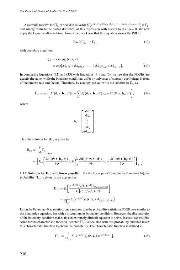
As a result, to solve forA0�t we need to solve forEt�e−Zt T �eCk0rT +k1x1�T +···+kmxm�T +km+1�T ��≡ B0�t
and simply evaluate the partial derivative of this expression with respect to C at C = 0. We nowapply the Feynman–Kac relation, from which we know that this equation solves the PDDE
In comparing Equations (32) and (33) with Equations (3 ) and (6), we see that the PDDEs areexactly the same, while the boundary conditions differ by only a set of constant coefficients in frontof the interest rate and factors. Therefore, by analogy, we can write the solution to B0�t as
B0�t = exp[A∗;4 '�b0�d∗�rt+
m∑i=1
B∗i ;4 '�b0�d∗�xi�t+C∗;4 '�b0�d∗�
]� (34)
where
b0 =
Ck0
Ck1
(((
CkmCkm+1
(
Thus the solution for A0�t is given by
A0�t =&
&CB0�t
∣∣∣∣C=0
={B0�t
[&A∗;4 '�b1�d∗�
&Crt+
m∑i=1
&B∗i ;4 '�b1�d∗�
&Cxi�t+
&C∗;4 '�b1�d∗�&C
]}C=0
(
1.1.2 Solution for �1� t with linear payoffs. For the linear payoff function in Equation (14), theprobability A1�t is given by the expression
A1�t = Et
[e−Zt T �fT r�x� '�1 fT r�x�'�≥K�
Et[e−Zt fT r�x� '�
] ]
= 1A0�t
Et[e−Zt T �fT r�x� '�1 fT r�x�'�≥K�
](
Using the Feynman–Kac relation, one can show that the probability satisfies a PDDE very similar tothe bond price equation, but with a discontinuous boundary condition. However, the discontinuityof the boundary condition makes this an extremely difficult equation to solve. Instead, we will firstsolve for the characteristic function, denoted A1� t , associated with this probability and then invertthis characteristic function to obtain the probability. The characteristic function is defined as
A1� t =1A0� t
Et[e−Zt T �fT r�x� '�ei.fT r�x�'�
]� (35)
230
Pricing Interest Rate Derivatives
where i =√−1 and . is a real-valued dummy variable. We can rewrite the characteristic functionas follows:
A1� t =1A0�t
1i
&
&.Et[e−Zt ei.fT r�x�'�
]= 1A0�t
1i
&
&.B1�t � (36)
where B1�t ≡ Et�e−Zt ei.fT r�x�'��.
We justify the interchange of the differentiation and expectation operators. We require that thedrift, diffusion, and jump components of the interest rate and factors satisfy the restrictions thatE��f r�x� '��k� be bounded for any k and E exp�CfT r�x� '��� be uniformly bounded at C = 0.The proof now follows:
&
&.Et[e−Zt T �ei.fT r�x�'�
]−Et[e−Zt T �ifT r�x� '�ei.fT r�x�'�]
= Et[e−Zt T �ei.+��fT r�x�'�
]−Et[e−Zt T �ei.fT r�x�'�]�
−Et[e−Zt T �ifT r�x� '�ei.fT r�x�'�
]= Et
[e−Zt T �ei.fT r�x�'�ei�fT r�x�'�−1�
]�
−Et[e−Zt T �ifT r�x� '�ei.fT r�x�'�
]= Et
[e−Zt T �ei.fT r�x�'�
ei�fT r�x�'�−1− i�fT r�x� '��
](
The integrand in the final equation can be shown to be dominated by 2�fT r�x� '�� and goes to 0with �; therefore the expected value goes to 0 by the dominated convergence theorem, and we havethe result that
&
&.Et[e−Zt T �ei.fT r�x�'�
]= Et[e−Zt T �ifT r�x� '�ei.fT r�x�'�
](
Note that B1�t is equivalent to B0�t evaluated at C = i.. Therefore, from the solution for B0�t inEquation (34), we have the solution for B1�t :
B1�t = exp[A∗;4 '�b1�d∗�rt+
m∑i=1
B∗i ;4 '�b1�d∗�xi�t+C∗;4 '�b1�d∗�
]� (37)
where
b1 =
i.k0
i.k1
(((
i.km+1
(
Then we have the solution for A1�t :
A1�t =1A0�t
{1iB1�t
[&A∗;4 '�b1�d∗�
&.rt+
m∑i=1
&B∗i ;4 '�b1�d∗�
&.xi�t+
&C∗;4 '�b1�d∗�&.
]}( (38)
231
The Review of Financial Studies / v 15 n 1 2002
1.1.3 Solution for �2� t with linear payoffs. For the linear payoff function in Equation (14), theprobability A2�t is given by the expression
A2�t = Et
[e−Zt T �1 fT r�x�'�≥K�
Et�e−Zt �
]= 1Pt'�
Et�e−Zt T �1 fT r�x�'�≥K��(
It is easy to show that A2�t satisfies a PDDE very similar to the bond price equation, but as withA1�t above, this PDDE has a discontinuity in its boundary condition which makes the equationextremely difficult to solve. Therefore, just as we solved for A1�t , we will solve for A2�t by firstcalculating the characteristic function A2�t associated with A2�t and then invert this characteristicfunction to obtain A2�t . The characteristic function is defined as
A2�t =1
Pt'�Et�e
−Zt T �ei.fT r�x�'��(
However, Et�e−Zt T �ei.fT r�x�'�� was calculated above in the derivation for A1�t :
Et[e−Zt T �ei.fT r�x�'�
]= B1�t (
Thus we have the result
A2�t =1
Pt'�B1�t
= 1Pt'�
exp[A∗;4 '�b1�d∗�rt+
m∑i=1
B∗i ;4 '�b1�d∗�xi�t+C∗;4 '�b1�d∗�
]�
where
b1 =
i.k0
i.k1
(((
i.kmi.km+1
(
2.2 Exponential linear payoffs
2.2.1 Solution for �0� t with exponential linear payoffs. From Equation (13),
A0�t = Et[e−Zt T �fT r�x� '�
]= Et
[e−Zt T � expk0rT +k1x1�T +· · ·+kmxm�T +km+1�T �
](
We now apply the Feynman–Kac relation, from which we know that this equation solves the PDDE
Notice that this is the exact same PDDE and boundary condition as Equations (32) and (33) withC= 1. Therefore we can write the solution for A0�t as
A0�t = exp[A∗;4 '�b0�d∗�rt+
m∑i=1
B∗i ;4 '�b0�d∗�xi�t+C∗;4 '�b0�d∗�
]� (41)
where
b0 =
k0
k1
(((
kmkm+1
(
2.2.2 Solution for �1� t with exponential linear payoffs. For the exponential linear payofffunction in Equation (19), the probability A1�t is given by the expression
A1�t = Et
[e−Zt T �fT r�x� '�1 fT r�x�'�≥K�
Et[e−Zt fT r�x� '�
] ]
= 1A0�t
Et[e−Zt T �fT r�x� '�1 fT r�x�'�≥K�
]= 1A0�t
Et[e−Zt T �fT r�x� '�1 log fT r�x�'�≥logK�
](
As with the linear payoff function, A1�t satisfies a PDDE similar to the bond price equation, butwith a discontinuous boundary condition. As we did withA1�t in the linear payoff function, we willfirst solve for the characteristic function, denoted A1�t , associated with this probability and theninvert this characteristic function to obtain the probability. The characteristic function is defined as
A1�t =1A0�t
Et[e−Zt T �fT r�x� '�ei. log fT r�x�'�
]= 1A0�t
Et[e−Zt T � exp
[1+ i.�k0rT +k1x1�T +· · ·+kmxm�T �
]]( (42)
From the Feynman–Kac relation, it is easy to see that A0�tA1�t satisfies
This is the same PDDE and boundary condition as Equations (32) and (33) with C = 1+ i..Therefore we can write the solution for A1�t as
A1�t =1A0�t
exp[A∗;4 '�b0�d∗�rt+
m∑i=1
B∗i ;4 '�b0�d∗�xi�t+C∗;4 '�b0�d∗�
]� (45)
233
The Review of Financial Studies / v 15 n 1 2002
where
b0 =
1+ i.�k0
1+ i.�k1
(((
1+ i.�km1+ i.�km+1
(
2.2.3 Solution for �2� t with exponential linear payoffs. For the exponential linear payofffunction in Equation (14), the probability A2�t is given by the expression
A2�t = Et
[e−Zt T �1 fT r�x�'�≥K�
Et�e−Zt T ��
]= 1Pt'�
Et[e−Zt T �1 log fT r�x�'�≥logK�
](
It is easy to show thatA2�t satisfies a PDDE very similar to the bond price equation, but as withA1�t
above, this PDDE has a discontinuity in its boundary condition, which makes the equation extremelydifficult to solve. Therefore, just as we solved for A1�t , we will solve for A2�t by first calculatingthe characteristic function,A2�t , associated withA2�t and then inverting this characteristic functionto obtain A2�t . The characteristic function is defined as
A2�t =1
Pt'�Et[e−Zt T �ei. log fT r�x�'�
]= 1Pt'�
Et[e−Zt T � exp�i.k0rT +k1x1�T +· · ·+kmxm�T +km+1�T ��
](
From the Feynman–Kac relation, it is easy to see that Pt'�A1�t satisfies
The boundary condition for this equation is ET = 1. Since this is the same PDDE and boundarycondition as Equations (3) and (6), but with d = d0, where
d′0 =
Ck0 −1Ck1
(((
CkmCkm+1
�
we can immediately calculate the solution for Et :
Et = exp[A∗;4 '�0�d0�rt+
m∑i=1
B∗i ;4 '�0�d0�xi�t+C∗;4 '�0�d0�
]( (52)
From Equation (51) we then have the solution for A0�t :
A0�t ={Et×
[&A∗;4 '�0�d0�
&Crt+
m∑i=1
&B∗i ;4 '�0�d0�
&Cxi�t+
&C∗;4 '�0�d0�
&C
]}C=0
( (53)
24 Given that e−CYt−Zt is bounded in time and the interest rate process r�x� is strong Markov, the dominatedconvergence theorem holds. Therefore the application of Fubini’s theorem is permitted here.
25 The justification for interchanging the differentiation and expectation operators follows along the lines of thatset out in the solution for A0�t in Section 1.1.1.
235
The Review of Financial Studies / v 15 n 1 2002
3.3.2 Solution for �1� t with integro-linear payoffs. For the integro-linear payoff, A1�t inEquation (27) is defined as
A1�t = Et
[e−Zt T �YtT �1 Yt T �≥K�Et�e
−Zt T �YtT ��
](54)
= 1A0�t
Et[e−Zt T �YtT �1 Yt T �≥K�
]( (55)
Using the Feynman–Kac relation,A1�t satisfies a PDDE similar to the bond price equation, but witha discontinuous boundary condition. Therefore we will first solve for the characteristic function,denoted A1�t , associated with this probability and then invert this characteristic function to obtainthe probability. The characteristic function is defined as
A1�t =1A0�t
Et[e−Zt T �YtT �e
i.Yt T �]( (56)
Notice, however, that Et[e−Zt T �+CYt T �
]was calculated already in the derivation for A0�t for
Equation (27). In this derivation Et[e−Zt T �+CYt T �
]was defined as Et and solved in Equation (52).
Therefore, we can write the solution to A1�t as26
A1� t =1A0�t
&E
&C
∣∣∣∣∣C=i.
= 1A0�t
{Et×
[&A∗;4 '�0�d0�
&Crt+
m∑i=1
&B∗i ;4 '�0�d0�
&Cxi�t+
&C∗;4 '�0�d0�
&C
]}C=i.
( (57)
3.3.3 Solution for �2� t with integro-linear payoffs. For the integro-linear payoff function inEquation (26), the probability A2�t is given by the expression
A2�t = Et
[e−Zt T �1 fT r�x�'�≥K�
Et[e−Zt T �
] ]
= 1Pt'�
Et[e−Zt T �1 Yt T �≥K�
](
It is easy to show thatA2�t satisfies a PDDE very similar to the bond price equation, but as withA1�t
above, this PDDE has a discontinuity in its boundary condition, which makes the equation extremelydifficult to solve. Therefore, just as we solved for A1�t , we will solve for A2�t by first calculatingthe characteristic function,A2�t , associated withA2�t and then inverting this characteristic functionto obtain A2�t . The characteristic function is defined as
A2� t =1
Pt'�Et[e−Zt T �ei.Yt T �
]= 1Pt'�
Et[e−Zt T �+i.Yt T �
](
26 The justification for interchanging the differentiation and expectation operators follows along the lines of thatset out in the solution for A1�t in Section 1.1.2.
236
Pricing Interest Rate Derivatives
However, Et[e−Zt T �+i.Yt T �
]≡Et , which has already been calculated in Equation (52). Therefore,we have the solution for the characteristic function:
A2�t =Et
Pt'�
∣∣∣∣∣C=i.
(58)
= 1Pt'�
exp[A∗;4 '�0�d0�rt+
m∑i=1
B∗i ;4 '�0�d0�xi�t+C∗;4 '�0�d0�
]C=i.
( (59)
Appendix B. Illustrative Callibration: The Vasicek Model
The interest rate process used is one with constant coefficients,
drt = ��O− rt� dt+1dWt�
where � is the coefficient of mean reversion, O is the long-run mean of the interest rate, and 1 isthe volatility coefficient for the driving Wiener process dWt . The estimation problem is a particularversion of the system in Equation (29):
min;
T∑t=1
N∑k=1
Gt�;'k��2
subject to � ; = ��O�1�
Gt�;'k�� = Y 'k�+1'�A'k�rt+C'k��
&A
&'= −�A−1� ∀'k�A0�= 0
&C
&'= 1
212A2 +�OA� ∀'k�C0�= 0(
We employed a panel of monthly data from the well-known McCulloch–Kwon database. Thisdata has zero-coupon yields for several maturities from 1 month to 20 years. We used the period8/1985–2/1991, because the database for this period is constructed from noncallable bonds and isnot confounded with options effects. The estimation exercise took a few seconds and resulted in thefollowing parameter estimates: [�= 1(6074�O= 0(0874�1 = 0(0408]. The estimated parametersmay be used directly in the pricing of interest rate derivatives.
ReferencesAhn, C. M., and H. E. Thompson, 1988, “Jump-Diffusion Processes and Term Structure of Interest Rates,”Journal of Finance, 43, 155–174.
Ahn, D.-H., and B. Gao, 1999, “A Parametric Nonlinear Model of Term Structure Dynamics,” Review ofFinancial Studies, 12, 721–762.
Ait-Sahalia, Y., 1996, “Testing Continuous-Time Models of the Interest Rate,” Review of Financial Studies, 9,385–426.
Attari, M., 1997, “Discontinuous Interest Rate Processes: An Equilibrium Model for Bond Option Prices,”working paper, University of Madison, Wisconsin; Ph.D. dissertation, University of Iowa.
Babbs, S. H., and N. J. Webber, 1995, “A Theory of the Term Structure with an Official Short Rate,” workingpaper, University of Warwick.
237
The Review of Financial Studies / v 15 n 1 2002
Bakshi, G., C. Cao, and Z. Chen, 1997, “Empirical Performance of Alternative Option Pricing Models,” Journalof Finance, 52, 2003–2049.
Bakshi, G., and D. Madan, 1997, “Average Rate Contingent Claims,” working paper, University of Maryland.
Bakshi, G., and D. Madan, 2000, “Spanning and Derivative Security Valuation,” Journal of Financial Economics,55, 205–238.
Balduzzi, P., G. Bertola, S. Foresi, and L. Klapper, 1998, “Interest Rate Targeting and the Dynamics ofShort-Term Rates,” Journal of Money, Credit and Banking, 30, 26–50.
Balduzzi, P., S. Das, and S. Foresi, 1998, “The Central Tendency: A Second Factor in Bond Yields,” Review ofEconomics and Statistics, 80, 60–72.
Barraquand, J., and T. Pudet, 1996, “Pricing of American Path-Dependent Contingent Claims,” MathematicalFinance, 6, 17–51.
Bates, D. S., 1996, “Jumps and Stochastic Volatility: Exchange Rate Processes Implicit in DM Options,” Reviewof Financial Studies, 9, 69–107.
Black, F., E. Derman, and W. Toy, 1991, “A One-Factor Model of Interest Rates and Its Application to TreasuryBond Options,” Financial Analysts Journal, January–February, 33–39.
Black, F., and M. Scholes, 1973, “The Pricing of Options and Corporate Liabilities,” Journal of PoliticalEconomy, 81, 637–654.
Bouaziz, L., E. Briys, and M. Crouhy, 1994, “The Pricing of Forward-Starting Asian Options,” Journal ofBanking and Finance, 18, 823–839.
Brandt, M., and P. Santa-Clara, 1998, “Simulated Likelihood Estimation of Diffusions with an Application toInterest Rates,” working paper, University of California, Los Angeles.
Brennan, M., and E. Schwartz, 1977, “A Continuous Time Approach to the Pricing of Bonds,” Journal ofBanking and Finance, 3, 133–155.
Brenner, R., R. Harjes, and K. Kroner, 1996, “Another Look at Models of the Short-Term Interest Rate,” Journalof Financial and Quantitative Analysis, 31, 85–107.
Brown, S., and P. Dybvig, 1986, “The Empirical Implications of the Cox, Ingersoll, Ross Theory of the TermStructure of Interest Rates,” Journal of Finance, 41, 616–628.
Burnetas, A. N., and P. Ritchken, 1996, “On Rational Jump-Diffusion Models in the Flesaker–HughstonParadigm,” working paper, Case Western Reserve University.
Carverhill, A. P., and L. J. Clewlow, 1990, “Valuing Average Rate (Asian) Options,” Risk, 3, 25–29.
Chacko, G., 1996, “A Stochastic Mean/Volatility Model of Term Structure Dynamics in a Jump-DiffusionEconomy,” unpublished manuscript, Harvard Business School.
Chacko, G., 1998. “Continuous-Time Estimation of Exponential Term Structure Models,” unpublishedmanuscript, Harvard Business School.
Chan, K. C., G. A. Karolyi, F. A. Longstaff, and A. B. Sanders, 1992, “An Empirical Comparison of AlternativeModels of the Short-Term Interest Rate,” Journal of Finance, 47, 1209–1228.
Conley, T. G., L. P. Hansen, E. G. J. Luttmer, and J. A. Scheinkman, 1997, “Short-Term Interest Rates asSubordinated Diffusions,” Review of Financial Studies, 10, 525–577.
Constantinides, G., 1992. “A Theory of the Nominal Term Structure of Interest Rates,” Review of FinancialStudies 5, 531–552.
Courtadon, G., 1982, “The Pricing of Options on Default Free Bonds,” Journal of Financial and QuantitativeAnalysis, 17, 75–100.
Cox, J. C., J. E. Ingersoll, and S. A. Ross, 1985, “A Theory of the Term Structure of Interest Rates,” Econometrica,1985, 385–407.
238
Pricing Interest Rate Derivatives
Dai, Q., and K. Singleton, 2000, “Specification Analysis of Affine Term Structure Models,” Journal of Finance,55, 1943–1978.
Dai, Q., and K. Singleton, 2001, “Expectation Puzzles, Time-Varying Risk Premia, and Dynamic Models of theTerm Structure,” working paper, Stanford University.
Das, S., 1997, “Discrete-Time Bond and Option Pricing for Jump-Diffusion Processes,” Review of DerivativesResearch, 1, 211–244.
Das, S., 1998 “The Surprise Element: Jumps in Interest Rates,” forthcoming in Journal of Econometrics.
Das, S., and S. Foresi, 1996, “Exact Solutions for Bond and Option Prices with Systematic Jump Risk,” Reviewof Derivatives Research, 1, 7–24.
Davydov, D., and V. Linetsky, 1999, “ The Valuation of Path-Dependent Options on One-Dimensional Diffu-sions,” working paper, University of Michigan.
De-Schepper, A., M. Teunen, M. Goovaerts, 1994, “An Analytical Inversion of a Laplace Transform Related toAnnuities,” Insurance: Mathematics and Economics, 14, 33–37.
Dewynne, J. N., and P. Wilmott, 1995, “Asian Options as Linear Complementary Problems: Analysis andFinite-Difference Solutions,” Advances in Options and Futures Research, 8, 145–173.
Duffie, D., 1996, “Dynamic Asset Pricing Theory, 2nd ed.,” Princeton University Press, Princeton, NJ.
Duffie, D., and P. Glyn, 1996, “Estimation of Continuous-Time Markov Processes Samples at Random TimeIntervals,” working paper, Stanford University.
Duffie, D., and R. Kan, 1996, “A Yield-Factor Model of Interest Rates,” Mathematical Finance, 6, 379–406.
Duffie, D., J. Pan, and K. Singleton, 2000, “Transform Analysis and Option Pricing for Affine Jump-Diffusions,”Econometrica, 68, 1343–1376.
Duffie, D., L. H. Pedersen, and K. Singleton, 2000, “Modeling Sovereign Yield Spreads: A Case Study ofRussian Debt,” working paper, Stanford University.
Duffie, D., and K. Singleton, 1997, “An Econometric Model of the Term Structure of Interest-Rate Swap Yields,Journal of Finance, 52, 1287–1321.
Dufresne, D., 1990, “The Distribution of a Perpetuity, with Applications to Risk Theory and Pension Funding,”Scandinavian Actuarial Journal, 90, 39–79.
Eydeland, A., and H. Geman, 1994, “Asian Options Revisited: Inverting the Laplace Transform,” mimeo,ESSEC.
Geman, H., and M. Yor, 1993, “Bessel Processes, Asian Options and Perpetuities,” Mathematical Finance, 3,349–375.
Gihman, I. I., and A. V. Skorohod, 1979, “Controlled Stochastic Processes,” Springer-Verlag, New York.
Gray, S. F., 1996, “Modeling the Conditional Distribution of Interest Rates as a Regime-Switching Process,”Journal of Financial Economics, 42, 27–62.
Heath, D., R. Jarrow., and A. Morton, 1992. “Bond Pricing and the Term Structure of Interest Rates: A NewMethodology for Contingent Claims Valuation,” Econometrica, 60, 77–106.
Heston, S., 1993, “A Closed-Form Solution for Options with Stochastic Volatility with Applications to Bondand Currency Options,” Review of Financial Studies, 6, 327–343.
Heston, S., and S. Nandi, 1999, “A Two-Factor Model for Pricing Bonds and Interest Rate Derivatives withGARCH Volatility: Analytical Solutions and Their Applications, working paper, Goldman Sachs.
Ho, T., and S. Lee, 1986, “Term Structure Movements and Pricing Interest Rate Contingent Claims,” Journalof Finance, 41, 1011–1029.
239
The Review of Financial Studies / v 15 n 1 2002
Hull, J., and A. White, 1990, “Pricing Interest-Rate Derivative Securities,” Review of Financial Studies, 3,573–592.
Jagannathan, R., and G. Sun, 1999, “Valuation of Swaps, Caps and Swaptions,” working paper, NorthwesternUniversity.
Jamshidian, F., 1989, “An Exact Bond Option Formula,” Journal of Finance, 44, 205–209.
Karatzas, I., and S. Shreve, 1988, “Brownian Motion and Stochastic Calculus,” Springer-Verlag, New York.
Kendall, M. G., J. K. Ord, and A. Stuart, 1987, “Kendall’s Advanced Theory of Statistics,” Oxford UniversityPress, New York.
Koedijk, K. G., F. G. J. A. Nissen, P. C. Schotman, and C. C. P. Wolff, 1996, “The Dynamics of the Short-TermInterest Rate Volatility Reconsidered,” unpublished manuscript, University of Limburg.
Kurtz, T. G., and P. E. Protter, 1996a, “Weak Convergence of Stochastic Integrals and Differential Equations.Probabilistic Models for Nonlinear Partial Differential Equations” (Montecatini Terme, 1995), 1–41, LectureNotes in Math, 1627, Springer, Berlin.
Kurtz, T. G., and P. E. Protter, 1996b. “Weak Convergence of Stochastic Integrals and Differential Equations II.Infinite-Dimensional Case. Probabilistic Models for Nonlinear Partial Differential Equations” (MontecatiniTerme, 1995), 197–285, Lecture Notes in Math, 1627, Springer, Berlin.
Leblanc, B., and O. Scaillet, 1998, “Path Dependent Options on Yields in the Affine Term Structure Model,”Finance and Stochastics, 2, 349–367.
Levin, A., 1998, “Deriving Closed-Form Solutions for Gaussian Pricing Models: A Systemic Time-DomainApproach,” International Journal of Theoretical and Applied Finance, 1, 349–376.
Longstaff, F., 1989, “A Nonlinear General Equilibrium Model of the Term Structure of Interest Rates,” Journalof Financial Economics, 23, 195–224.
Longstaff, F. A., 1995. “Hedging Interest Rate Risk with Options on Average Interest Rates,” Journal of FixedIncome, March, 37–45.
Longstaff, F. A., and E. Schwartz, 1992, “Interest Rate Volatility and the Term Structure: A Two-Factor GeneralEquilibrium Model,” Journal of Finance, 48, 1259–1282.
Merton, R., 1973, “Rational Theory of Option Pricing,” Bell Journal of Economics and Management Science,4, 141–183.
Naik, V., and M. H. Lee, 1993, “Yield Curve Dynamics with Discrete Shifts in Economic Regimes: Theory andEstimation,” working paper, University of British Columbia.
Pardoux, E., 1997, “Generalized Discontinuous Backward Stochastic Differential Equations,” in N. El Karouiand L. Mazliak (eds), Backward Stochastic Differential Equations, Pitman Research Notes in MathematicsSeries Addison Wesley, Longman, UK.
Pritsker, M., 1998, “Nonparametric Density Estimation of Tests of Continuous Time Interest Rate Models,”Review of Financial Studies, 11, 449–488.
Protter, P. E., 1990, “Stochastic Integration and Differential Equations,” Springer-Verlag, New York.
Scott, L., 1995, “Pricing Stock Options in a Jump-Diffusion Model with Stochastic Volatility and Interest Rates:Applications of Fourier Inversion Methods,” working paper, University of Georgia.
Shephard, N. G., 1991, “From Characteristic Function to Distribution Function: A Simple Framework for theTheory,” Econometric Theory, 7, 519–529.