rsta.royalsocietypublishing.org Research Cite this article: Baptist S, Hepburn C. 2013 Intermediate inputs and economic productivity. Phil Trans R Soc A 371: 20110565. http://dx.doi.org/10.1098/rsta.2011.0565 One contribution of 15 to a Discussion Meeting Issue ‘Material efficiency: providing material services with less material production’. Subject Areas: materials science Keywords: material intensity, material efficiency, intermediate inputs, productivity, total factor productivity, economic growth Author for correspondence: Cameron Hepburn e-mail: [email protected]Intermediate inputs and economic productivity Simon Baptist and Cameron Hepburn Vivid Economics Ltd., London School of Economics, London, UK Many models of economic growth exclude materials, energy and other intermediate inputs from the production function. Growing environmental pressures and resource prices suggest that this may be increasingly inappropriate. This paper explores the relationship between intermediate input intensity, productivity and national accounts using a panel dataset of manufacturing subsectors in the USA over 47 years. The first contribution is to identify sectoral production functions that incorporate intermediate inputs, while allowing for heterogeneity in both technology and productivity. The second contribution is that the paper finds a negative correlation between intermediate input intensity and total factor productivity (TFP)—sectors that are less intensive in their use of intermediate inputs have higher productivity. This finding is replicated at the firm level. We propose tentative hypotheses to explain this association, but testing and further disaggregation of intermediate inputs is left for further work. Further work could also explore more directly the relationship between material inputs and economic growth— given the high proportion of materials in intermediate inputs, the results in this paper are suggestive of further work on material efficiency. Depending upon the nature of the mechanism linking a reduction in intermediate input intensity to an increase in TFP, the implications could be significant. A third contribution is to suggest that an empirical bias in productivity, as measured in national accounts, may arise due to the exclusion of intermediate inputs. Current conventions of measuring productivity in national accounts may overstate the productivity of resource-intensive sectors relative to other sectors. 1. Introduction Since the industrial revolution, energy and material costs have fallen dramatically and rapid economic c 2013 The Author(s) Published by the Royal Society. All rights reserved. on July 7, 2018 http://rsta.royalsocietypublishing.org/ Downloaded from
Transcript
rsta.royalsocietypublishing.org
ResearchCite this article: Baptist S, Hepburn C. 2013Intermediate inputs and economicproductivity. Phil Trans R Soc A 371: 20110565.http://dx.doi.org/10.1098/rsta.2011.0565
One contribution of 15 to a Discussion MeetingIssue ‘Material efficiency: providing materialservices with less material production’.
Subject Areas:materials science
Keywords:material intensity, material efficiency,intermediate inputs, productivity, total factorproductivity, economic growth
Intermediate inputs andeconomic productivitySimon Baptist and Cameron Hepburn
Vivid Economics Ltd., London School of Economics, London, UK
Many models of economic growth exclude materials,energy and other intermediate inputs from theproduction function. Growing environmental pressuresand resource prices suggest that this may beincreasingly inappropriate. This paper explores therelationship between intermediate input intensity,productivity and national accounts using a paneldataset of manufacturing subsectors in the USA over47 years. The first contribution is to identify sectoralproduction functions that incorporate intermediateinputs, while allowing for heterogeneity in bothtechnology and productivity. The second contributionis that the paper finds a negative correlationbetween intermediate input intensity and total factorproductivity (TFP)—sectors that are less intensivein their use of intermediate inputs have higherproductivity. This finding is replicated at the firmlevel. We propose tentative hypotheses to explain thisassociation, but testing and further disaggregation ofintermediate inputs is left for further work. Furtherwork could also explore more directly the relationshipbetween material inputs and economic growth—given the high proportion of materials in intermediateinputs, the results in this paper are suggestive offurther work on material efficiency. Depending uponthe nature of the mechanism linking a reductionin intermediate input intensity to an increase inTFP, the implications could be significant. A thirdcontribution is to suggest that an empirical bias inproductivity, as measured in national accounts, mayarise due to the exclusion of intermediate inputs.Current conventions of measuring productivity innational accounts may overstate the productivity ofresource-intensive sectors relative to other sectors.
1. IntroductionSince the industrial revolution, energy and materialcosts have fallen dramatically and rapid economic
development has occurred along an energy- and material-intensive growth path. Over thetwentieth century, despite a quadrupling of the population and a 20-fold increase in economicoutput, available material resources became more plentiful, relative to manufactured capitaland labour, and technological advances continued to drive down their prices. Economists oftenomitted natural and environmental resources from production functions altogether, as capital andlabour were more important determinants of output, and measurement issues meant that it wasdifficult to glean insights from data on material inputs.
This material-intensive economic model has substantially increased pressure on (i)environmental resources, such as the climate, fisheries and biodiversity, and (ii) natural resourcesand commodities. In a variety of domains, the so-called ‘planetary boundaries’ appear to havebeen exceeded [1]. Commodity prices have increased by almost 150 per cent in real terms overthe last 10 years, after falling for much of the twentieth century [2], and 44 million people fell intopoverty because of rising food prices in the second half of 2010 [3].
Current environmental and resource pressures seem likely to increase as the humanpopulation swells from 7 to 9–10 billion and as the number of middle-class consumers growsfrom 1 to 4 billion people [4].1 If increases in living standards are to occur without social andenvironmental dislocation, major improvements in the efficiency and productivity with whichwe use materials and other intermediate inputs will be required.
Given these pressures, omitting intermediate inputs, particularly material inputs, fromeconomic production functions, as is common in macroeconomic modelling, appears increasinglyunwise. Production functions with capital and labour as the sole ‘factors of production’ may havebeen justified a century ago; it was a sensible modelling strategy to ignore materials, given theirrelative abundance and the absence of useful data. However, results in this paper indicate that itis worth exploring the possibility that omitting material inputs may lead to biased estimates ofproductivity.2
This paper explores the important relationship between intermediate inputs (of whichmaterials are a major component) and productivity. Understanding of the role of materials inthe economy is currently limited by a number of elements of the standard economic approach toproductivity measurement. The two most important limitations, discussed further in §2, are thefollowing.
— The use of value added aggregate measures. Value added is defined as the value of totaloutput minus the cost of raw materials, energy and other intermediate inputs. Thismeasure is useful for analyses of economy-wide income and economic growth becausethe sum of the value added across all entities in the economy equates with total grossdomestic product (GDP). However, value-added measures have two major drawbacksin working with materials. First, they tend to require the assumption of constant anduniform use of materials over time and across sectors. Second, they exclude material useas an explanatory factor in generating national income and productivity.
— Conceptual and practical limitations on data on ‘material’ inputs. Data collected for nationalaccounts on purchases of raw materials are not normally separated out from data onpurchases of other physical intermediate inputs, such as components, or sometimes evenfrom all intermediate inputs. This is partly due to conceptual problems of distinguishingbetween raw materials and processed intermediate components.
1Middle-class consumers are defined as those with daily per capita spending of between $10 and $100 in purchasing powerparity terms [4].2Omitting materials also reflects an inaccurate assumption about scarcity and value. For instance, this type of assumption hasled to the adoption of national accounts, which do not include genuine balance sheets measuring wealth and other stocks;the focus is almost entirely on flows, although earlier studies [5–7] provide notable exceptions. One consequence is that manynations, such as Australia, effectively account for the extraction of natural resources as a form of income, rather than as apartial asset sale.
on July 7, 2018http://rsta.royalsocietypublishing.org/Downloaded from
In this paper, we focus primarily on addressing the first limitation. We do so by using a ‘gross-output’ production function, rather than a ‘value-added’ production function. This restricts ourability to draw robust conclusions on an economy-wide scale—because many of the outputsof one firm are inputs to another firm—but it does allow us to account for heterogeneity inboth intermediate input intensity and productivity across economic sectors. Generalizing theanalysis in this way places additional demand on the data required for empirical analysis,which means that it is not possible to simultaneously and comprehensively address the secondlimitation without compromising on statistical reliability. Accordingly, our empirical strategy isfirst to establish robustly the relationship between economic productivity and the wider notionof intermediate inputs, as used in national accounts. The application to a narrower definition ofintermediate inputs is left to future work when the required data becomes available.
While we would prefer to distinguish material inputs alone, data limitations mean that in thispaper an empirical analysis based solely on material inputs was not possible, and intermediateinputs are used instead. Intermediate inputs are defined as the sum of the real values of physicalintermediate inputs, energy and purchased services (calculated by applying National Bureau ofEconomic Research (NBER) deflators to the nominal monetary values of each input).3
The primary analysis of the paper uses data on industrial subsectors from the USA over the 47years from 1958 to 2005. Material costs largely declined over this period until just after 2000, atwhich point they increased rapidly [8]. A secondary analysis employs firm-level data from SouthKorea to demonstrate that the results are not an artefact of sectoral composition. We also usethe South Korean data to empirically explore the relationship between gross-output and value-added measures of productivity. In both cases, we estimate or use production functions thatexplicitly account for the role of intermediate inputs, and then explore the association betweenthe intermediate intensity of production (defined as the cost share of intermediate inputs in totalcost) and total factor productivity (TFP). Productivity is commonly defined as a ratio of a volume(not value) measure of output (such as gross output or value added) to a volume measure ofinput use [9]. In contrast, TFP accounts for impacts on total output that are not explained by the(measured) inputs, including capital and labour, as discussed in §2 below.
The analysis in this paper indicates that lower intermediate input intensity is positivelyassociated with higher TFP, both across the US subsectors and across the South Korean firms.In other words, firms and industries that employ modes of production that use more labour andfewer intermediate inputs appear to have overall higher TFP. The results in this paper suggestthat policies which encourage less intermediate input-intensive sectors or reduce the intermediateinput intensity of production may lead to increases in average productivity. Policies to promotematerial efficiency (or more general reductions in material intensity) should thus be explored,given the possible microeconomic and macroeconomic benefits.
The paper proceeds as follows. Section 2 sets out the theoretical economics of materialefficiency, reviewing research that has employed production functions incorporating materials,in some form or other, and exploring the relationship with economic productivity. This sectionalso provides the theoretical basis for the empirical part of the paper, presented in §3. Section 3describes the data, methodology and results of our analysis of US manufacturing subsectorsand South Korean firms. Section 4 explores the policy implications of our analysis and§5 concludes.
2. Theoretical economics of material efficiencyMaterial efficiency is often defined as the provision of more goods and services with fewermaterials [10]. As foreshadowed, the definition of materials within the engineering literature isoften different to that employed in economics. Engineers and scientists have tended to definematerials to mean physical inputs, such as iron ore and steel, often measured in units of mass. By
3This follows the definitions used in the primary dataset we employ. While intermediate inputs are not disaggregated furtherin the dataset used for the main analysis, the US Annual Survey of Manufactures indicates that intermediate inputs arecomprised around 72 per cent physical inputs, 23 per cent services and 5 per cent energy inputs.
on July 7, 2018http://rsta.royalsocietypublishing.org/Downloaded from
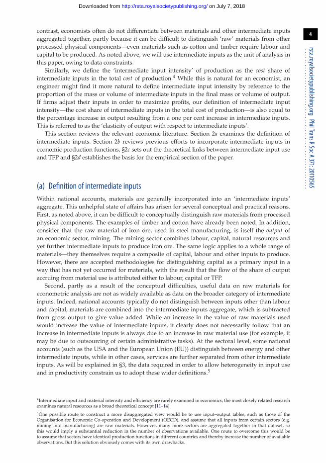
contrast, economists often do not differentiate between materials and other intermediate inputsaggregated together, partly because it can be difficult to distinguish ‘raw’ materials from otherprocessed physical components—even materials such as cotton and timber require labour andcapital to be produced. As noted above, we will use intermediate inputs as the unit of analysis inthis paper, owing to data constraints.
Similarly, we define the ‘intermediate input intensity’ of production as the cost share ofintermediate inputs in the total cost of production.4 While this is natural for an economist, anengineer might find it more natural to define intermediate input intensity by reference to theproportion of the mass or volume of intermediate inputs in the final mass or volume of output.If firms adjust their inputs in order to maximize profits, our definition of intermediate inputintensity—the cost share of intermediate inputs in the total cost of production—is also equal tothe percentage increase in output resulting from a one per cent increase in intermediate inputs.This is referred to as the ‘elasticity of output with respect to intermediate inputs’.
This section reviews the relevant economic literature. Section 2a examines the definition ofintermediate inputs. Section 2b reviews previous efforts to incorporate intermediate inputs ineconomic production functions, §2c sets out the theoretical links between intermediate input useand TFP and §2d establishes the basis for the empirical section of the paper.
(a) Definition of intermediate inputsWithin national accounts, materials are generally incorporated into an ‘intermediate inputs’aggregate. This unhelpful state of affairs has arisen for several conceptual and practical reasons.First, as noted above, it can be difficult to conceptually distinguish raw materials from processedphysical components. The examples of timber and cotton have already been noted. In addition,consider that the raw material of iron ore, used in steel manufacturing, is itself the output ofan economic sector, mining. The mining sector combines labour, capital, natural resources andyet further intermediate inputs to produce iron ore. The same logic applies to a whole range ofmaterials—they themselves require a composite of capital, labour and other inputs to produce.However, there are accepted methodologies for distinguishing capital as a primary input in away that has not yet occurred for materials, with the result that the flow of the share of outputaccruing from material use is attributed either to labour, capital or TFP.
Second, partly as a result of the conceptual difficulties, useful data on raw materials foreconometric analysis are not as widely available as data on the broader category of intermediateinputs. Indeed, national accounts typically do not distinguish between inputs other than labourand capital; materials are combined into the intermediate inputs aggregate, which is subtractedfrom gross output to give value added. While an increase in the value of raw materials usedwould increase the value of intermediate inputs, it clearly does not necessarily follow that anincrease in intermediate inputs is always due to an increase in raw material use (for example, itmay be due to outsourcing of certain administrative tasks). At the sectoral level, some nationalaccounts (such as the USA and the European Union (EU)) distinguish between energy and otherintermediate inputs, while in other cases, services are further separated from other intermediateinputs. As will be explained in §3, the data required in order to allow heterogeneity in input useand in productivity constrain us to adopt these wider definitions.5
4Intermediate input and material intensity and efficiency are rarely examined in economics; the most closely related researchexamines natural resources as a broad theoretical concept [11–14].5One possible route to construct a more disaggregated view would be to use input–output tables, such as those of theOrganisation for Economic Co-operation and Development (OECD), and assume that all inputs from certain sectors (e.g.mining into manufacturing) are raw materials. However, many more sectors are aggregated together in that dataset, sothis would imply a substantial reduction in the number of observations available. One route to overcome this would beto assume that sectors have identical production functions in different countries and thereby increase the number of availableobservations. But this solution obviously comes with its own drawbacks.
on July 7, 2018http://rsta.royalsocietypublishing.org/Downloaded from
(b) Intermediate inputs in economic production functionsMaterials have occasionally been included in the production functions of theoretical economicgrowth models exploring the sustainability of economic growth. For instance, theory indicatesthat sustainable growth may be possible, provided that human-made capital and otherreplacement resources substitute for depleted natural resources [11]. Technological advancesand capital accumulation might also offset declining natural resources, provided the rate oftechnological advance is high enough [14].6 Empirically, however, it appears that currentinvestments in human and manufactured capital by several countries are insufficient to offsetthe depletion of natural capital [6].
The increases in energy prices in the 1970s stimulated much research into energy consumptionand its relationship with gross output [15,16], including work on input–output formulations [17].This led to an interest in directly accounting for intermediate inputs such as materials, energyand services, in the production function. Since then, many studies have estimated KLEM (capital,labour, energy and materials) and KLEMS (capital, labour, energy, materials and services)production functions, for data as early as 1947 [18].7 These various research efforts provide auseful starting point for this paper, but do not provide any investigation of the relationshipbetween material inputs and productivity.
More generally, rather than material use, research in this broad area has focused instead eitheron the relationship between productivity and energy consumption [16,24,26,27] or on energyprices [15,28,29]. For instance, empirical studies of the US economy have shown long-term trendsin the relationship between energy use and productive efficiency [16,26], and Jorgenson [30]found that declining energy intensity is correlated with higher productivity in manufacturingindustries in the USA, although this may not have been caused by improvements in energyefficiency. However, no research has considered whether such results for energy use are observedfor material use.
(c) Total factor productivityProductivity has different definitions in different contexts. In national accounts, it is typicallymeasured as the ratio of outputs, measured by value (not mass or volume), to inputs, measured byvalue (not mass or volume) [9]. In the economic growth literature, there are various productivitymeasures, including ‘labour productivity’—value added per worker—and as ‘TFP’, which isthe constant term in the production function (loosely, that part of the output which cannot beexplained after accounting for the application of defined inputs, including capital and labour).
TFP is not directly measured, but emerges as the residual in the regression of total output onmeasured inputs. So, for instance, if important inputs are omitted, measured TFP may be biasedupwards. Measures of TFP from the early economic growth literature [31,32] were subsequentlyused as the basis for analysis of productivity growth across firms, industries and countries [33–36].Early studies tended to estimate TFP by representing the production process using a value-addedfunction [37], in which value added, V, is related to gross output, Y, and intermediate inputs,M, as
V = Y − M. (2.1)
A value-added estimation approach is commonly employed to determine productivity. Thisis partly because it is consistent with aggregation up to the economy-wide scale, but alsobecause of a lack of data available to base the analysis on gross output. However, as notedabove, the value-added approach has several limitations [9]. By definition, because it adjusts
6The specific requirement is that the rate of technical change divided by the discount rate is greater than the output elasticityof resources [14].7It has long been argued that energy is an additional and significant input in the production function, and that it cannot simplybe substituted for by other inputs [12,19–22]. Ayres argues that ‘exergy services’—energy inputs multiplied by an overallconversion efficiency—are a key driver of economic growth, and that incorporating exergy as a factor of production increasesthe explanatory power of traditional production functions [23–25]. This literature is relevant here because it demonstrates theimpact of omitting relevant inputs from the production function.
on July 7, 2018http://rsta.royalsocietypublishing.org/Downloaded from
for all intermediate inputs, such as materials, it does not take into account the contribution ofinputs other than capital and labour. The value-added approach therefore implicitly assumes thattechnical change only operates on capital and labour inputs, and that all other inputs are usedin fixed proportions. Generally, the hypothesis that technology affects only primary inputs hasnot held up to empirical verification, and technical change has been observed to be a complexprocess, with some changes affecting all factors of production simultaneously, while other typesof change affect individual factors of production separately [38]. Furthermore, the value-addedapproach does not correspond directly to a specific model of production [39]. When data allow,the gross-output approach will be preferred [40] for some purposes, such as those in this paper,while the value-added approach will be preferred for others.
The relationship between TFP and ‘technology choice’—the choice of the mix of labour, capitaland intermediate inputs, represented formally by the coefficients of the production function—has not, to our knowledge, been explored in the literature. Yet, determining whether there is arelationship between the input intensity of different production techniques and productivity isimportant because it would help firms and policy makers to increase productivity. This paperattempts to conduct such an analysis using empirical methods, examining the relationshipbetween TFP and the intermediate input intensity of production, as measured by the outputelasticity of intermediate inputs. The next section explains our methodological strategy.
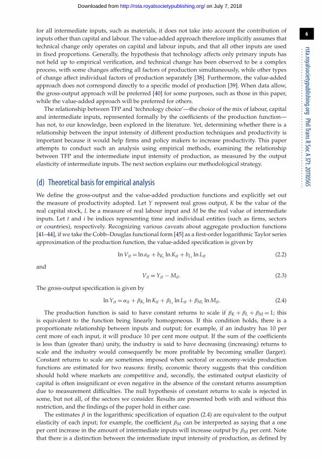
(d) Theoretical basis for empirical analysisWe define the gross-output and the value-added production functions and explicitly set outthe measure of productivity adopted. Let Y represent real gross output, K be the value of thereal capital stock, L be a measure of real labour input and M be the real value of intermediateinputs. Let t and i be indices representing time and individual entities (such as firms, sectorsor countries), respectively. Recognizing various caveats about aggregate production functions[41–44], if we take the Cobb–Douglas functional form [45] as a first-order logarithmic Taylor seriesapproximation of the production function, the value-added specification is given by
The production function is said to have constant returns to scale if βK + βL + βM = 1; thisis equivalent to the function being linearly homogeneous. If this condition holds, there is aproportionate relationship between inputs and output; for example, if an industry has 10 percent more of each input, it will produce 10 per cent more output. If the sum of the coefficientsis less than (greater than) unity, the industry is said to have decreasing (increasing) returns toscale and the industry would consequently be more profitable by becoming smaller (larger).Constant returns to scale are sometimes imposed when sectoral or economy-wide productionfunctions are estimated for two reasons: firstly, economic theory suggests that this conditionshould hold where markets are competitive and, secondly, the estimated output elasticity ofcapital is often insignificant or even negative in the absence of the constant returns assumptiondue to measurement difficulties. The null hypothesis of constant returns to scale is rejected insome, but not all, of the sectors we consider. Results are presented both with and without thisrestriction, and the findings of the paper hold in either case.
The estimates β in the logarithmic specification of equation (2.4) are equivalent to the outputelasticity of each input; for example, the coefficient βM can be interpreted as saying that a oneper cent increase in the amount of intermediate inputs will increase output by βM per cent. Notethat there is a distinction between the intermediate input intensity of production, as defined by
on July 7, 2018http://rsta.royalsocietypublishing.org/Downloaded from
the coefficients of the production function, and the physical volume of intermediate inputs thata firm or sector uses. The production function determines the output that would be expectedto be generated from a certain set of inputs; but the exact choice of input factor ratios will bedetermined by the reactions of a profit-maximizing firm, subject to the fixed constraints of factorprices, and the production function. The ratio of intermediate inputs to other factors of production(e.g. intermediate inputs per worker) will vary with factor prices, even if the production functionis fixed (i.e. lower intermediate input prices will mean more intermediate input use, but not adifferent intermediate input intensity using our measure).
The value-added production function is valid if all intermediate inputs, including materials,are separable from other inputs, there is perfect competition, no changes in the rate of outsourcingand homogeneous technology. Biases from value-added production functions can arise if anyof these conditions is not met, which is why employing the gross-output production functionto derive econometric estimates of TFP is preferred for our analysis. Furthermore, we showthat there is a systematic divergence between measures of TFP based upon the gross-outputand value-added production functions, and that the size of this divergence is a function of theintermediate input intensity of production. Value added is an important concept, not only becauseit is the dominant specification for accounting for cross- and within-country income differences,but also because it forms the analytical underpinning for national accounting of GDP. Value-added measures also capture the extent to which an industry generates national income (ratherthan output). It is therefore of great interest to understand the nature and extent of any impact onproductivity measurements from the exclusion of intermediate inputs.
Consider the relationship between the gross output and value-added measures of TFP: whatif the gross-output model is given by equation (2.4) but we estimate equation (2.2)? The first-order conditions for profit maximization can be derived by taking the marginal product of eachfactor, i.e. the derivatives of the three-factor gross-output production function in equation (2.4),and setting these equal to factor prices and solving the three resulting simultaneous equations forthe input quantities of K, L and M. Letting pF represent the price of factor F and letting A = eα , wehave
M =[
YA
(pK
βK
)βK(
pL
βL
)βL(
βM
pM
)βK+βL]1/(βK+βL+βM)
. (2.5)
Without loss of generality, we assume constant returns to scale for simplicity and writeequation (2.5) as M = γ (Y/A) (note that prices and the output elasticities are taken to be fixedso γ is a constant). In order to understand the bias in the coefficients in equation (2.2), we want toexpress the true model of production (firms physically produce gross output, e.g. tonnes of steel,rather than value added, which is rather an accounting construct derived from gross output)in a form that corresponds to the value-added model and then compare coefficients. Repeatedsubstitution of equation (2.4) into equation (2.2), using equations (2.3) and (2.5), and suppressingsubscripts for notational clarity, gives
ln V = ln Y + ln(
1 − MY
)
= ln A + βK ln K + βL ln L + βM ln M + ln(
1 − γ
A
)= ln A + βK ln K + βL ln L + βM[ln Y − ln A + ln γ ] + ln
(1 − γ
A
)
= ln A + βM
1 − βMln γ + ln
(1 − γ
A
)+ βK
1 − βMln K + βL
1 − βMln L. (2.6)
In our three-factor model with constant returns to scale, the relationship between the value-addedand gross-output coefficients is therefore
ln a = ln A + βM
1 − βMln γ + ln
(1 − γ
A
), bK = βK
βK + βLand bL = βL
βK + βL. (2.7)
on July 7, 2018http://rsta.royalsocietypublishing.org/Downloaded from
Equation (2.7) shows that estimates of TFP from a value-added production function will bebiased estimates of gross-output TFP and the size of this bias will be increasing in βM. Value addedis a useful summary statistic for discussing the distribution of income and in deriving measuresof productivity that reflect the extent to which economy-wide income cannot be explained bythe accumulation of capital and labour. However, the omission of intermediate inputs and theresultant divergence in measures of TFP means that the underlying productivity of the productionprocess is better measured using the gross-output production function.
In the empirical work that follows in §3, we investigate the observed pattern betweenunderlying productivity and intermediate input intensity using the gross-output specification.
3. Empirical analysisIn this section, we use sectoral and firm-level data to investigate the hypothesis that a higherintermediate input intensity is associated with lower underlying TFP. We also use firm-leveldata to show that estimates of value-added TFP are indeed divergent in the manner derived inequation (2.7).
It is worth emphasizing the stringent data requirements in order to relax the conventionalassumptions that intermediate inputs enter the production function in an identical way forall sectors and that productivity is unrelated to intermediate input use. In order to obtain asingle data point with these generalizations, it is necessary to estimate a production function.The estimated production function coefficients and the estimate of TFP then provide a singleobservation, which can be used to investigate the question of the nature of the relationshipbetween intermediate input intensity and TFP. Therefore, it is necessary to collect enough datato estimate each relevant production function, and then to repeat the process a sufficient numberof times in order to have enough data points for the ultimate analysis. Note also that each ofthe observations in the ultimate analysis must be sufficiently related such that it is sensible tocompare them.
The dataset we have employed satisfies these stringent data requirements. In order to obtainenough observations to allow for heterogeneity to investigate the relationship between input useand TFP at the sectoral level, we have had to accept a level of aggregation of inputs that is higherthan we would prefer (i.e. intermediate inputs rather than materials).
(a) DataWe investigate our hypothesis primarily using the NBER-CES manufacturing industry database,and full details of variable definitions and database construction are available from the website ofthe NBER [46]. The dataset is a panel of 473 manufacturing industries defined to the six-digit level(based upon NAICS codes) from 1958 to 2005. The data are unbalanced in that some industriesenter or leave manufacturing due to a change in the industry coding structure in 1996, but all datahave been coded so that they are consistent with the current sectoral definitions.
The dataset contains annual industry-level data on employment and hours, nominal value ofshipments, value added, capital stock and intermediate inputs, along with price indices for sales,capital stock and intermediate inputs. Firm gross output is constructed as the value of shipmentsplus the change in inventories, using the price index for shipments to deflate into real values.Hours worked are calculated by multiplying total employment by the average hours worked byproduction workers: the hours of non-production workers are not available and so we assumethat non-production workers in a sector put in the same number of hours as production workers.Real value added is calculated by using the price indices for shipments and materials, with theprice index for shipments being used as a deflator for inventories. Two NAICS industries—334 111(computers) and 334 413 (semiconductors)—are excluded from the analysis due to difficulties inconstructing accurate price deflators. We do not have data on human capital, such as averageeducation of workers, at the subsectoral level but, in the context of models with heterogeneoustechnology, human capital can be controlled by the inclusion of intercept and time trend termsunder plausible conditions [47].
on July 7, 2018http://rsta.royalsocietypublishing.org/Downloaded from
(b) Specification of intermediate input intensity and parameter heterogeneityIn this analysis, ‘technology’ is used to refer to the set of coefficients βK, βL, βM, while TFP isdefined as the constant term α, and is allowed to vary over time and across sectors throughthe inclusion of binary dummy variables. The least restrictive assumption we could make ontechnology in this context would be to allow each six-digit industry to have its own set ofproduction function coefficients, possibly varying over time. However, this would have thedisadvantage of reducing the sample size available for each estimated production function, wouldnot allow for the exploitation of the panel dimension of the dataset and, most importantly, wouldnot allow unrestricted TFP evolution as there would be insufficient observations to include yeardummies. We therefore allow for technological heterogeneity at the three-digit level (i.e. theindustries defined in table 1), and assume that every six-digit subsector of a three-digit industryhas common technology. Technology is also held to be fixed within a three-digit industry overtime.8 This is, of course, more restrictive than allowing technology to differ by six-digit subsector,but less restrictive than estimating a production function at the level of aggregate manufacturingor of the aggregate economy. It has recently been argued that the focus in the literature on cross-country and cross-sectoral production functions on matters of endogeneity and specificationhas neglected the important possible role of parameter heterogeneity [47]. This paper presentsevidence that one critical element of this heterogeneity is in the role of intermediate inputsin production.
8This, along with the inclusion of time dummies, means that secular trends in productivity and the share of intermediateinputs are not the cause of our results; rather, they are driven by the cross-sectional variation between sectors.
on July 7, 2018http://rsta.royalsocietypublishing.org/Downloaded from
If prices of inputs and technology are taken to be exogenous and there is perfect competitionand constant returns to scale, then the first-order conditions of profit maximization inequation (2.4) imply that the share of intermediate inputs in total cost will be equal to βM.An augmented condition holds if these restrictions do not apply. While only the exogeneityrestrictions are imposed in our modelling, we use this result as a motivation for our empiricaldefinition of intermediate input intensity: a sector is said to be more intensive if the coefficient βM
is higher, and this paper aims to investigate the relationship between TFP and intermediate inputintensity by estimating production functions for different subsectors of US manufacturing.9
(c) Estimation strategyWe employ econometric methods to estimate the parameters of an aggregate production functionand express productivity in terms of the estimated parameters. Our approach is different tothe standard ‘growth accounting’ approach [38,48]. The growth accounting approach is touse a non-parametric technique that weights different types or qualities of factors by incomeshares [49,50]. While the growth accounting approach has often been preferred due to its lessstringent data requirements, it requires five key assumptions in order to be valid. First, it assumesa stable relationship between inputs and outputs at various levels of the economy, with marginalproducts that are measurable by observed factor prices [51]. Second, the production functionused must exhibit constant returns to scale [49]. Third, the approach assumes that producersbehave efficiently, minimizing costs and maximizing profits [49]. Fourth, the approach requiresperfectly competitive markets within which participants are price takers who can only adjustquantities [49]. Fifth, a particular form of technical change must be assumed.
In contrast, the econometric methods we employ do not require the a priori assumptionsof the growth accounting method. Rather, they enable these assumptions to be tested [52].Equations (2.2) and (2.4) are estimated using a range of econometric techniques.10 Identificationproblems [41] can be overcome using the plausible and widely made assumption that the pricesfor inputs and outputs vary across subsectors.11
We employ four different econometric techniques: ordinary least squares (OLS), the standardpanel data fixed effect (FE) estimator, the mean group (MG) estimator [54] and the commoncorrelated effects mean group estimator (CCEMG) [55]. These latter two estimators allow for moregeneral forms of cross-sectional and time-series dependence, as well as forms of heterogeneityin the error structure. The OLS estimator will be valid if statistical error for each observationis independently and normally distributed. A FE estimator relaxes this assumption by allowingfor common time-invariant factors within a subsector. The MG estimator will yield consistentestimates so long as there is not heterogeneity in unobserved variables and errors are stationary.The CCEMG estimator allows for heterogeneity in the unobservables and allows for cross-sectional dependence resulting from unobserved factors common between sectors (e.g. commonshocks affecting more than one subsector). These issues would require a fuller treatment in order
9Equation (2.4) shows why material or intermediate input per unit of output is not an appropriate measure to investigate ourhypotheses, as an increase in TFP (i.e. α) will trivially decrease material per unit of output.10The literature on estimating production functions, particularly in the context of panel data with a long time-series dimensionis rapidly evolving. One of the key difficulties in this literature has been finding a specification and an estimation methodthat achieve both economic and econometric regularity [38]. A recent survey of the state of production function estimationis given by Eberhardt & Teal [47], which contains a full discussion of the different estimation techniques available and theconditions required for each of them to produce unbiased and efficient estimates of the true underlying parameters.11If all inputs are costlessly adjustable and chosen optimally then, if prices are common, a Cobb–Douglas production functionwill be unidentified [53]. Taking the first derivative of a Cobb–Douglas production function leads to a first-order conditionwhere quantities are functions of prices and the (sector or firm-specific) TFP term. So, with common prices, inputs are allcollinear with the TFP term and so are unidentified. This problem is mitigated in the presence of adjustment costs or wheresectors face different factor prices. Note that input prices faced by sectors can still differ, even if one were to believe that inputmarkets are perfect. For example, the effective price of labour will differ with commuting distances; the price of capital willdiffer with proximity and expertise of repair and maintenance firms, which themselves may be sector specific, or with creditconstraints. Contracts for the supply of raw materials will contain prices that will vary depending on when the contract wassigned and the relative use of spot or forward markets. Transport costs for physical intermediate inputs will also be firmand sector specific, and so on. Even if prices were to be identical between sectors, the identification problem can be solvedprovided adjustment costs between inputs differ by firm or sector, as would be expected.
on July 7, 2018http://rsta.royalsocietypublishing.org/Downloaded from
to precisely identify the production function parameters and to make possible statements about acausal impact of intermediate input intensity on TFP, and so we do not make claims of causalityin this paper. Rather, we seek to demonstrate that intermediate input intensity is related to TFPand that the relationship is robust to a number of different econometric approaches.
The key results of this paper—that sectors with higher intermediate input intensity tend tohave lower levels of TFP and that value-added estimates of TFP have a bias that is increasing inintermediate input intensity—are robust to these choices of estimation technique. We present theresults from all four estimation methods graphically, in each case with and without imposing theassumption of constant returns to scale. For the sake of brevity, only the OLS results are presentedin table form in the main body of the paper, but the results from the other estimators in table formare available from the authors upon request.
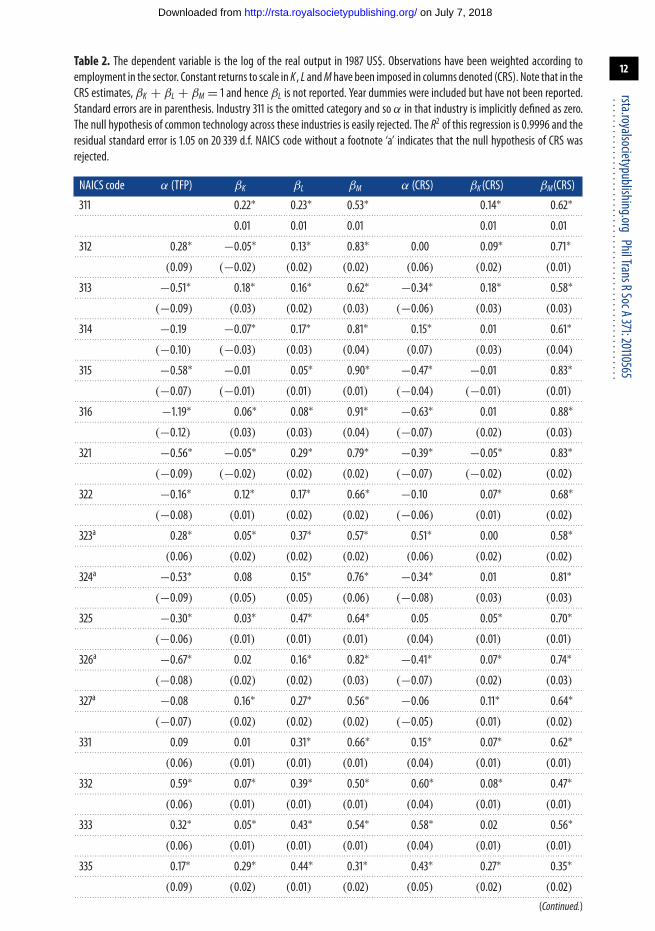
(d) Results and discussionThe results from the OLS regression for each of the 20 industries considered are presented intable 2. The production function coefficients are generally plausible: the coefficients on labour andintermediate inputs are all positive, as are the majority of those on capital. Owing to difficultiesin the valuation of capital stock, it is not uncommon for some estimates of βK to be negativeor poorly identified, and constant returns to scale are often imposed to achieve regularity giventhat the condition should be satisfied in an industry in equilibrium.12 For example, Burnside [56]concludes that constant returns to scale is probably an appropriate restriction for US sectoral-level production functions. Both the restricted and unrestricted results are presented here, andthe conclusions follow regardless.
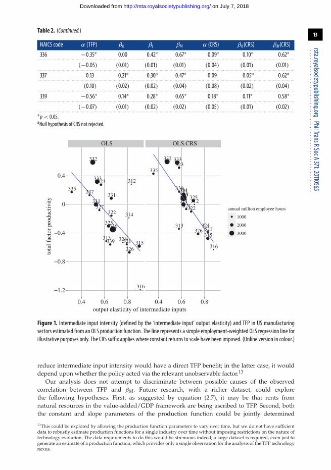
While our primary interest is in the pattern between the sets of coefficients α, βK, βL and βM,we first describe their absolute estimates to give a feel for the results. The highest intermediateinput intensity (as measured by βM) is observed in the apparel (315) and leather (316) sectors,where intermediate inputs account for around 90 per cent of total inputs; the lowest is found inelectrical equipment (335) and furniture (337) manufacturing, where the share is under 50 percent. TFP is highest in fabricated metal products (332) and machinery (333) and lowest in leatherproducts (316) and plastics and rubber (326).
The relationship between the intermediate intensity of an industry and its TFP is shown infigure 1. There is a clear relationship in the pattern of coefficients across industries: those sectorswith a higher intermediate input intensity tend to have lower TFP. This pattern is repeated for theFE estimator, shown in figure 2, and the MG and CCEMG estimators, shown in figure 3.
The β coefficients of the production function sum to a quantity close to unity for all industrieswhere the estimation is unrestricted. Therefore, a negative pattern between βM and TFP impliesthat there is likely a positive pattern between TFP and at least one of the other coefficients. Figure 4depicts the observed pattern between the labour output elasticity and TFP using the results fromtable 2. There is a strong positive relationship: sectors that are more intensive in their use of labourinputs tend to have higher TFP. There is no clear pattern in relation to capital intensity, which isnot shown for brevity. The fact that labour-intensive sectors have higher TFP and intermediateinput-intensive sectors have lower TFP is reminiscent of the (controversial) ‘double dividend’hypothesis that replacing labour taxes with environmental taxes might reduce the costs imposedby the tax system [57].
Because TFP is, by its very nature, capturing unobserved elements of the production process, itis not possible to infer from this analysis the precise nature of the relationship between the two. Itmay be the case that reducing intermediate input intensity causes changes in unobserved factorsthat lead to increase TFP directly, or it may be that changes in an associated unobservable factorresult both in a lower share of intermediate inputs and higher TFP. In the former case, policies to
12Recall that because α is defined as the constant term in a logarithmic equation, negative values simply refer to levels of TFPof between zero and one and are not cause for concern.
on July 7, 2018http://rsta.royalsocietypublishing.org/Downloaded from
Table 2. The dependent variable is the log of the real output in 1987 US$. Observations have been weighted according toemployment in the sector. Constant returns to scale in K , L andM have been imposed in columns denoted (CRS). Note that in theCRS estimates, βK + βL + βM = 1 and hence βL is not reported. Year dummies were included but have not been reported.Standard errors are in parenthesis. Industry 311 is the omitted category and so α in that industry is implicitly defined as zero.The null hypothesis of common technology across these industries is easily rejected. The R2 of this regression is 0.9996 and theresidual standard error is 1.05 on 20 339 d.f. NAICS code without a footnote ‘a’ indicates that the null hypothesis of CRS wasrejected.
0.4 0.6 0.8 0.4 0.6 0.8output elasticity of intermediate inputs
tota
l fac
tor
prod
uctiv
ity
annual million employee hours
1000
2000
3000
Figure 1. Intermediate input intensity (defined by the ‘intermediate input’ output elasticity) and TFP in US manufacturingsectors estimated from an OLS production function. The line represents a simple employment-weighted OLS regression line forillustrative purposes only. The CRS suffix applies where constant returns to scale have been imposed. (Online version in colour.)
reduce intermediate input intensity would have a direct TFP benefit; in the latter case, it woulddepend upon whether the policy acted via the relevant unobservable factor.13
Our analysis does not attempt to discriminate between possible causes of the observedcorrelation between TFP and βM. Future research, with a richer dataset, could explorethe following hypotheses. First, as suggested by equation (2.7), it may be that rents fromnatural resources in the value-added/GDP framework are being ascribed to TFP. Second, boththe constant and slope parameters of the production function could be jointly determined
13This could be explored by allowing the production function parameters to vary over time, but we do not have sufficientdata to robustly estimate production functions for a single industry over time without imposing restrictions on the nature oftechnology evolution. The data requirements to do this would be strenuous indeed; a large dataset is required, even just togenerate an estimate of a production function, which provides only a single observation for the analysis of the TFP technologynexus.
on July 7, 2018http://rsta.royalsocietypublishing.org/Downloaded from
Figure 2. Intermediate input intensity (defined by the ‘intermediate input’ output elasticity) and TFP in US manufacturingsectors estimated using the FE estimator. The line represents a simple OLS regression line for illustrative purposes only. Notethat all subsectors of each three-digit sector have the same intermediate input intensity coefficient by construction. The CRSsuffix applies where constant returns to scale have been imposed. (Online version in colour.)
fundamental parameters of the production function. Third, the pattern of outsourcing and verticalintegration both between sectors and within a sector over time might differ in such a way that issystematically related to TFP. This list of possible drivers of the correlation is not exhaustive.
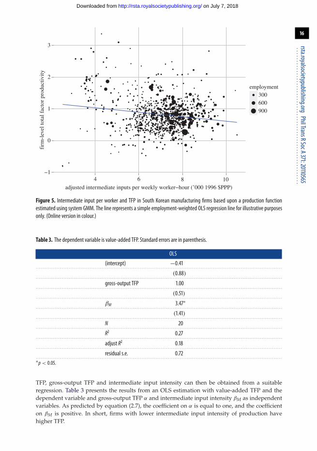
We conduct a further piece of analysis to address a possible concern that the sectoralrelationship is an artefact of the aggregation of firms, and that any variation can be solelyaccounted for by sectoral composition alone rather than by intermediate input intensity. If theinverse relationship between TFP and intermediate input intensity also holds at the firm level aswell as the sectoral level, this would suggest that results are not merely an artefact of sectoralcomposition. Figure 5 presents some indicative evidence at the firm level that this relationshipbetween intermediate input intensity and TFP is not purely a sectoral one. The dataset usedis a panel of 863 medium-sized manufacturing firms14 from South Korea observed for threeyears from 1996 to 1998 from a survey conducted by the World Bank, see Hallward-Driemeieret al. [58] for a full description of the dataset (the ideal comparison, a panel of US firms from thesectors and years of the sectoral data was not accessible). TFP is calculated using a productionfunction previously estimated using this data [59], and intermediate input intensity is calculatedas intermediate inputs per unit of labour input.15
Finally, we return to the value-added specification and the hypothesis derived in equation (2.7)that value-added estimates of TFP are biased estimates of underlying TFP, and that the size of thisbias is increasing in intermediate input intensity. Value-added TFP is calculated by estimatingequation (2.2) using OLS with constant returns to scale imposed (because income shares mustnecessarily sum to one in the value-added framework). The relationship between value-added
14From the textile, garments, machinery, electronics and wood products sectors.
15Because a single production function was estimated for this dataset, βM is the same for all firms, so an alternative measureof factor intensity was required. Using intermediate inputs per unit of output could not be used because this could generate aspurious relationship: a hypothetical exogenous increase in TFP would increase output per intermediate input, even if therewas no change in the manner in which intermediate inputs were used in the production process.
on July 7, 2018http://rsta.royalsocietypublishing.org/Downloaded from
0.6 0.7 0.5 0.6 0.7 0.8output elasticity of intermediate inputs
gros
s-ou
tput
TFP
annual million employee hours
1000
2000
3000
Figure 3. Intermediate input intensity (defined by the ‘intermediate input’ output elasticity) and TFP in US manufacturingsectors estimated using theMG and CCEMG techniques. The line represents a simple OLS regression line for illustrative purposesonly. Sectors with 10 or fewer groups have been excluded as these estimators perform poorly in such situations. The CRS suffixapplies where constant returns to scale have been imposed. (Online version in colour.)
labour output elasticity
tota
l fac
tor
prod
uctiv
ity
−1.0
0.1 0.2 0.3 0.4 0.1 0.2 0.3 0.4
−0.5
0
0.5
OLS
311
332
312
335
313
337
314
315
316
321
322
323
324
325
326
327
331
333
336
339
OLS.CRS
311
313
315321
322
323
324
325
326
327
331
332333
335
312336
314337
316
339annual million employee hours
500
1000
1500
2000
2500
3000
3500
Figure 4. Labour intensity and TFP in USmanufacturing sectors estimated fromanOLS production function. The line representsa simple employment-weighted OLS regression line for illustrative purposes only. (Online version in colour.)
on July 7, 2018http://rsta.royalsocietypublishing.org/Downloaded from
Figure 5. Intermediate input per worker and TFP in South Korean manufacturing firms based upon a production functionestimated using system GMM. The line represents a simple employment-weighted OLS regression line for illustrative purposesonly. (Online version in colour.)
Table 3. The dependent variable is value-added TFP. Standard errors are in parenthesis.
TFP, gross-output TFP and intermediate input intensity can then be obtained from a suitableregression. Table 3 presents the results from an OLS estimation with value-added TFP and thedependent variable and gross-output TFP α and intermediate input intensity βM as independentvariables. As predicted by equation (2.7), the coefficient on α is equal to one, and the coefficienton βM is positive. In short, firms with lower intermediate input intensity of production havehigher TFP.
on July 7, 2018http://rsta.royalsocietypublishing.org/Downloaded from
4. Policy implicationsSome of the policy implications from our empirical results depend upon the conceptual basisfor the relationship discovered between intermediate input intensity and TFP; that is, theprecise nature of the unobserved factors driving TFP which are associated with intermediateinput intensity. We find at least two possibilities plausible. First, because TFP captures allunobservables, if there are more positive spillovers from one factor of production thanothers, a higher intensity in that factor of production will be associated with higher TFP. Forinstance, it may be that there are positive externalities from human capital accumulation in theworkforce [60]. This would explain why TFP is higher in industries that are more labour intense.Other things equal (or indeed if capital use involves some positive externalities), it would followthat intermediate input-intensive industries, with lower intensity of capital and labour inputs,will be associated with lower TFP. Whether policies to reduce intermediate input use directlywould themselves lead to increased TFP would depend upon the nature of the externalities.
Second, by analogy to Porter & van der Linde [61], it may be that firms that search for waysof lowering their intermediate input intensity also have higher TFP, either because the questfor reducing intermediate inputs creates other opportunities that are captured by the firms or,perhaps more likely, firms that are well managed are able to both reduce their intermediate inputintensity and also deliver greater TFP as a result of superior management practices.
The broad observation that lower intermediate input intensity is associated with higherTFP potentially is consistent with at least three specific policy recommendations (and there arepotentially many others). First, irrespective of causality underpinning our results, it seems likelythat productivity could be improved, and environmental and resource pressure reduced, by areduction in the subsidies spent annually on materials and resource use. Such subsidies provideincentives for firms to increase intermediate input intensity that, as we have seen, is associatedwith lower TFP. Perhaps US$1 trillion is spent every year on directly subsidizing the consumptionof resources [62]. This includes subsidies of approximately $400 billion on energy [63], around$200–300 billion of equivalent support on agriculture [64], very approximately US$200–300 billionon water [62] and approximately US$15–35 billion on fisheries [65]. To take one perverse example,subsidies worth 0.5 per cent of EU GDP are spent annually on providing tax relief for companycars, which increases greenhouse gas emissions by between 4 and 8 per cent [66].
While these direct subsidies are vast, they pale in comparison with the indirect subsidies inthe form of natural assets that governments have failed to properly price. The indirect subsidyassociated with lack of payments for biodiversity loss and other environmental costs is estimatedat perhaps as much as $6.6 trillion [67].16 Of this, US$1 trillion, very approximately, takes theform of subsidies for the use of the atmosphere as a sink for greenhouse gas emissions [62].By comparison, global GDP is around US$60 trillion at 2010 prices. Various countries, includingNorway, Brazil and Australia have imposed explicit resource taxes, but taxes in one area do notundo the problems created by subsidies in another.
Second, productivity might be increased by other policies focused on reducing materialintensity, beyond reducing perverse subsidies. One obvious example of this would be shifting thetax base away from labour, the factor input that correlates with higher TFP, and towards materialsand resources, the factor correlated with lower TFP. This follows regardless of whether the resultsin this paper are driven by sectoral composition effects, or whether the relevant unobservablesare directly related to material use within sectors. Taxing environmental externalities is obviouslyeconomically rational, as is taxing mineral rents [68], irrespective of other considerations. Forinstance, in contrast to the very substantial tax rates on labour, only a very small proportion of taxrevenues are raised globally from taxation of resource use. For instance, even in OECD countries,environmental taxes comprise only 6 per cent of total tax revenues based on 2008 data; in the USA,the proportion is around 3 per cent, in the UK, it is around 6 per cent, whereas in The Netherlands,it is above 10 per cent [69].
16This estimate should be viewed with high methodological scepticism. Nevertheless, it can be taken as an indication that thescale of the ‘subsidy’ is extremely large.
on July 7, 2018http://rsta.royalsocietypublishing.org/Downloaded from
Third, our results suggest that value-added measures of productivity, as commonly embodiedin national accounting frameworks, may overstate the underlying gross-output productivity ofintermediate input-intensive sectors. As data from national accounts inform economic policy, itis possible that this systematic difference has led to policies which have sub-optimally increasedthe size of material-intensive sectors in the economy. National accounts should also endeavourto measure material use as well. If possible, material use should be further decomposed toseparate energy and services from other natural resources and raw materials from purchasedcomponents.
5. ConclusionThis paper investigated the relationship between intermediate input intensity and TFP. Thiswas achieved through the estimation of gross-output production functions for US industrialsubsectors allowing for subsectoral heterogeneity in both of the key variables of interest: TFPand intermediate input intensity. The main limitations of the analysis, from the perspective ofan interest in material use, because of stringent data requirements, were that results were basedon data on intermediate inputs, of which materials form a major (but not exclusive) part, andwere at the subsector level. A robustness check—using firm-level data—did not overturn the keyconclusions.
There were three key results from our empirical analysis. First, there is a negative relationshipbetween intermediate input intensity and TFP in the data examined. Second, there is a positiverelationship between labour intensity and TFP. Those sectors that are more intensive in their useof humans, rather than raw materials and other intermediate inputs, have higher levels of TFP,which means that a greater level of output is achieved from any given level of inputs. Firm-levelevidence indicates that this relationship may not just be a result of sectoral composition. However,the determination of a causal impact within a sector of a reduction in intermediate input intensityincreasing TFP is left to future research, as is further narrowing to a definition of material inputsalone. Third, value-added measures of productivity, inherent in the national accounts of almostall countries, may systematically overstate the output-based productivity of material-intensivesectors. Changing national accounting frameworks to include material inputs, and improving thescope and quality of their measurement, should be a priority if natural resources are to be usedefficiently and productivity maximized.
We are grateful to Julian Allwood, Alex Bowen, Eric Beinhocker, Nicola Brandt, John Daley, Markus Eberhardt,Simon Dietz, Ross Garnaut, Elizabeth Garnsey, Carlo Jaeger, Alan Kirman, Eric Neumayer, Carl Obst, AlanSeatter and three anonymous referees, among others, for useful discussions about the issues addressed in thispaper. We are extremely grateful to Hyunjin Kim for outstandingly diligent and helpful research assistance.C.H. is grateful to the Grattan Institute in Melbourne, Australia, for hospitality while working on the paper.C.H. also thanks the ESRC Centre for Climate Change Economics and Policy and the Grantham ResearchInstitute at the LSE for support. All errors remain our own.
References1. Rockström J. et al. 2009 A safe operating space for humanity. Nature 461, 472–475.
(doi:10.1038/461472a)2. Dobbs R, Oppenheim J, Thompson F. 2011 A new era for commodities. McKinsey Quarterly,
1–3 November 2011.3. Ivanic M, Martin W, Zaman H. 2011 Estimating the short-run poverty impacts of the 2010–11
surge in food prices. World Bank Policy Research Working Paper 5633, Washington, DC.4. Kharas H. 2010 The emerging middle class in developing countries. OECD Development
Centre Working Paper 285, January, Paris, France.5. World Bank. 1997 Expanding the measure of wealth: indicators of environmentally sustainable
development, vol. 17. ESD Studies and Monographs Series. Washington, DC: World Bank.6. Arrow K et al. 2004 Are we consuming too much? J. Econ. Perspect. 18, 147–172. (doi:10.1257/
0895330042162377)
on July 7, 2018http://rsta.royalsocietypublishing.org/Downloaded from
7. Arrow K, Dasgupta P, Goulder L, Mumford KJ, Oleson K. 2012 Sustainability and themeasurement of wealth. Environ. Dev. Econ. 17, 317–353. (doi:10.1017/S1355770X12000137)
8. Garnaut R, Howes S, Jotzo F, Sheehan P. 2008 Emissions in the platinum age: the implicationsof rapid development for climate-change mitigation. Oxf. Rev. Econ. Policy 24, 377–401.(doi:10.1093/oxrep/grn021)
9. OECD. 2001 Measuring productivity: Measurement of aggregate and industry-level productivitygrowth. Paris, France: OECD.
10. Allwood J, Ashby M, Gutowski T, Worrell E. 2011 Material efficiency: a white paper. Resour.Conserv. Recycl. 55, 362–381. (doi:10.1016/j.resconrec.2010.11.002)
11. Solow R. 1974 The economics of resources or the resources of economics. Am. Econ. Rev. 64,1–14.
12. Georgescu-Roegen N. 1975 Energy and economic myths. South. Econ. J. 41, 347–381.(doi:10.2307/1056148)
13. Dasgupta P, Heal G. 1979 The optimal depletion of exhaustible resources. Rev. Econ. Stud. 41,3–28. (doi:10.2307/2296369)
14. Stiglitz JE. 1974 Growth with exhaustible natural resources: efficient and optimal growthpaths. Rev. Econ. Stud. 41, 123–137. (doi:10.2307/2296377)
15. Berndt ER. 1982 Energy price increases and the productivity slowdown in United Statesmanufacturing. Federal Reserve Bank, Boston, MA, USA.
16. Schurr S. 1984 Energy use, technological change, and productive efficiency: aneconomic-historical interpretation. Annu. Rev. Energy 9, 409–425. (doi:10.1146/annurev.eg.09.110184.002205)
17. Hannon B, Blazeck T, Kennedy D, Illyes R, 1983 A comparison of energy intensities: 1963, 1967and 1972. Resour. Energy 5, 83–102. (doi:10.1016/0165-0572(83)90019-1)
18. Berndt E, Khaled M. 1979 Parametric productivity measurement and choice among flexiblefunctional forms. J. Political Econ. 87, 1220–1245. (doi:10.1086/260833)
19. Costanza R. 1980 Embodied energy and economic valuation. Science 210, 1219–1224.(doi:10.1126/science.210.4475.1219)
20. Daly HE. 1991 Elements of an environmental macroeconomics. In Ecological economics (ed.R Costanza), pp. 32–46. Oxford, UK: Oxford University Press.
21. Cleveland CJ, Ruth M. 1997 When, where, and by how much do biophysical limits constrainthe economic process?; a survey of Nicholas Georgescu-Roegen’s contribution to ecologicaleconomics. Ecol. Econ. 22, 203–223. (doi:10.1016/S0921-8009(97)00079-7)
22. Stern D. 2011 The role of energy in economic growth. Ecol. Econ. Rev. 1219, 26–51.23. Ayres R, Warr B. 2005 Accounting for growth: the role of physical work. Struct. Change Econ.
Dyn. 16, 181–209. (doi:10.1016/j.strueco.2003.10.003)24. Ayres R. 2007 On the practical limits to substitution. Ecol. Econ. 61, 115–128. (doi:10.1016/
j.ecolecon.2006.02.011)25. Ayres R, Warr B. 2009 The economic growth engine: how energy and work drive material prosperity.
Cheltenham, UK: Edward Elgar Publishing.26. Schurr S. 1985 Productive efficiency and energy use. Ann. Oper. Res. 2, 229–238. (doi:10.1007/
BF01874741)27. Schurr S, Netschert B. 1960 Energy and the American economy, 1850–1975. Baltimore, MA: Johns
Hopkins University Press.28. Brown S, Yucel M. 2002 Energy prices and aggregate economic activity: an interpretative
survey. Q. Rev. Econ. Finance 42, 193–208. (doi:10.1016/S1062-9769(02)00138-2)29. Hamilton J. 1983 Oil and the macroeconomy since world war II. J. Political Econ. 91, 228–248.
(doi:10.1086/261140)30. Jorgenson D. 1984 The role of energy in productivity growth. Energy 5, 11–26.
(doi:10.5547/ISSN0195-6574-EJ-Vol5-No3-2)31. Tinbergen J. 1942 Zur theorie der langfristigen wirtschaftsentwicklung (on the theory of long-
term economic growth). Weltwirtschaftliches Arch. 55, 511–549.32. Solow R. 1957 Technical change and the aggregate production function. Rev. Econ. Stat. 39,
312–320. (doi:10.2307/1926047)33. Kravis I. 1976 A survey of international comparisons of productivity. Econ. J. 86, 1–44.
(doi:10.2307/2230949)34. Link A. 1987 Technological change and productivity growth. Chur, Switzerland: Taylor & Francis.35. Christensen L, Cummings D, Jorgenson D. 1980 Economic growth, 1947–73; an international
comparison. In New developments in productivity measurement (eds JW Kendrick, BN Vaccara),pp. 595–698. Cambridge, MA: NBER.
on July 7, 2018http://rsta.royalsocietypublishing.org/Downloaded from
36. Maddison A. 1987 Growth and slowdown in advanced capitalist economies: techniques andquantitative assessment. J. Econ. Lit. 25, 649–698.
37. Beaudreau B. 1995 The impact of electric power on productivity: a study of US manufacturing1950–1984. Energy Econ. 17, 231–236. (doi:10.1016/0140-9883(95)00025-P)
38. Feng G, Serletis A. 2008 Productivity trends in U.S. manufacturing: evidence from the NQ andaim cost functions. J. Econ. 142, 281–311. (doi:10.1016/j.jeconom.2007.06.002)
39. Bruno M. 1978 Duality, intermediate inputs and value added. In Production economics: adual approach to theory and applications, vol. 2, ch. 1 (eds M Fuss, D McFadden), pp. 1–16.Amsterdam, The Netherlands: Elsevier.
40. Basu S, Fernald JG. 1995 Are apparent productive spillovers a figment of specification error?J. Monetary Econ. 35, 165–188. (doi:10.1016/0304-3932(95)01208-6)
41. Koopmans TC. 1949 Identification problems in economic model construction. Econometrica 17,125–144. (doi:10.2307/1905689)
42. Fisher FM. 1969 The existence of aggregate production functions. Econometrica 37, 553–577.(doi:10.2307/1910434)
43. Johansen L. 1972 Production functions. Amsterdam, The Netherlands: North Holland.44. Sato K. 1975 Production functions and aggregation. Amsterdam, The Netherlands: North
Holland.45. Cobb CW, Douglas PH. 1928 A theory of production. Am. Econ. Rev. 18, 139–165.46. Becker RA, Gray WB. 2009 NBER-CES manufacturing industry database. The National Bureau
of Economic Research. See www.nber.org/data/nbprod2005.html.47. Eberhardt M, Teal F. 2011 Econometrics for grumblers: a new look at the literature on
cross-country growth empirics. J. Econ. Surveys 25, 109–155. (doi:10.1111/j.1467-6419.2010.00624.x)
48. Jorgenson DW, Griliches Z. 1967 The explanation of productivity change. Rev. Econ. Stud. 34,349–383. (doi:10.2307/2296675)
49. Mawson P, Carlaw K, McLellan N. 2003 Productivity measurement: alternative approachesand estimates. New Zealand Treasury Working Paper, Wellington, New Zealand.
50. Hulten C. 2010 Growth accounting. Amsterdam, The Netherlands: Elsevier.51. Barro RJ. 1999 Notes on growth accounting. J. Econ. Growth 4, 119–137. (doi:10.1023/
A:1009828704275)52. Berndt E, Wood D. 1975 Technology, prices, and the derived demand for energy. Rev. Econ.
Stat. 57, 259–268. (doi:10.2307/1923910)53. Bond S, Söderbom M. 2005 Adjustment costs and the identification of Cobb–
Douglas production functions. The Institute for Fiscal Studies Working Paper Series,WP05/04, London, UK.
54. Pesaran M, Smith R. 1995 Estimating long-run relationships from dynamic heterogenouspanels. J. Econ. 68, 79–113. (doi:10.1016/0304-4076(94)01644-F)
55. Pesaran M. 2006 Estimation and inference in large heterogenous panels with a multifactorerror structure. Econometrica 74, 967–1012. (doi:10.1111/j.1468-0262.2006.00692.x)
56. Burnside C. 1996 Production function regressions, returns to scale and externalities.J. Monetary Econ. 37, 177–201. (doi:10.1016/S0304-3932(96)90033-1)
57. Goulder LH. 1994 Environmental taxation and the double dividend: a reader’s guide. Int. TaxPublic Finance 2, 157–183. (doi:10.1007/BF00877495)
58. Hallward-Driemeier M, Iarossi G, Sokoloff KL. 2002 Exports and manufacturing productivityin East Asia: a comparative analysis with firm-level data. NBER Working PaperSeries 8894, Cambridge, MA.
59. Baptist S. 2008 Technology, human capital and efficiency in manufacturing firms. DPhil thesis,Oxford University, Oxford, UK.
60. Acemoglu D. 1996 A microfoundation for social increasing returns in human capitalaccumulation. Q. J. Econ. 111, 779–804. (doi:10.2307/2946672)
61. Porter ME, van der Linde C. 1995 Toward a new conception of the environment–competitiveness relationship. J. Econ. Perspect. 9, 97–118. (doi:10.1257/jep.9.4.97)
62. Dobbs R, Oppenheim J, Thompson F, Brinkman M, Zornes M, 2011 Resource revolution: meetingthe world’s energy, materials, food and water needs. McKinsey Global Institute, London, UK.
63. International Energy Agency (IEA). 2011 World energy outlook 2011. Paris, France: IEA.64. OECD. 2011 Agricultural policy monitoring and evaluation 2011: OECD countries and emerging
economies. Paris, France: OECD.
on July 7, 2018http://rsta.royalsocietypublishing.org/Downloaded from
65. United Nations Environment Programme (UNEP). 2008 Fisheries subsidies: a critical issue fortrade and sustainable development at the WTO. Geneva, Switzerland: UNEP.
66. Copenhagen Economics. 2010 Company car taxation. Working paper no. 22, European Union,Luxembourg.
67. United Nations Environment Programme Finance Initiative Principles for ResponsibleInvestment. 2011 Universal ownership: why environmental externalities matter toinstitutional investors. Principles for Responsible Investment Association and United NationsEnvironment Programme Finance Initiative. See http://unepfi.org/fileadmin/document.
68. Garnaut, Clunies-Ross A. 1983 Taxation of mineral rents. Oxford, UK: Oxford University Press.69. OECD. 2010 Taxation, innovation and the environment. Paris, France: OECD.
on July 7, 2018http://rsta.royalsocietypublishing.org/Downloaded from