Internal Management Directive Library/IMD-DevConLimitsFacilities.pdfIMD: Developing Concentration...

Developing Concentration Limits at Permitted Solid Waste Facilities

Internal Management Directive

Last updated: February 2011 By: Audrey Eldridge DEQ Solid Waste Program 11-LQ-033

3 3

IMD: Developing Concentration Limits at Permitted Solid Waste Facilities February 2011

Table of Contents

Introduction ............................................................................................................. 5

Overview .................................................................................................................. 6

Chapter 1: Selecting Monitoring Wells and Parameters for Long-Term Monitoring and Compliance .................................................................................. 7

Chapter 2: Managing Groundwater Quality Data ........................................... 15

Chapter 3. Concentration Limits for Permitted Facilities ............................... 22

Chapter 4. Using Statistics to Establish Concentration Limits ....................... 24

Chapter 5. Conducting Long-Term Compliance Monitoring.......................... 31

Appendix A: Parameter Groups – Solid Waste Facilities ................................. 35

Appendix B – Boxplot ........................................................................................... 37

Appendix C - Shapiro Wilk Example ................................................................. 38

Appendix D – Non Parametric Comparison with Pooled Data ....................... 40

Attachment 1 – Associated Tables from US EPA Unified Guidance, 2009

3

4 4


Acronyms/Abbreviations

AL Action limit CLV Concentration limit varianceDAF Dilution attenuation factorDEQ Department of Environmental QualityEMP Environmental monitoring planEPA Environmental Protection AgencyERPC EPA reference power curvesGWQPR Groundwater quality protection rules (OAR 340‐40)HCU Hydrogeologic compliance unitIMD Internal management directiveIPA Informal preliminary assessmentIQR Interquartile rangeLOD Limit of detectionLOQ Limit of quantificationMCL Maximum concentration limitMRL Method reporting limitMS Matrix spike NELAP National Environmental Laboratory Accreditation Program ORELAP Oregon Environmental Laboratory Accreditation Program PA Preliminary assessmentPOC Parameters of concernPSCL Permit specific concentration limitQA/QC Quality assurance/quality controlROS Regression on order statisticsRPD Relative percent differenceRSD Relative standard deviationSSL Site specific limitSW Solid waste SWFPR Site wide false positive rateTDS Total dissolved solidsUPL Upper prediction limitVOC Volatile organic compound

4

5 5


Introduction

The purpose of this internal management directive (IMD) is to promote consistent interpretation and implementation of the Department of Environmental Quality (DEQ or the ‘Department’) regulations governing groundwater monitoring at permitted solid waste facilities in Oregon. Specifically, this directive will provide technically sound methods for the DEQ Solid Waste hydrogeologists to assist permittees with their permit compliance, including: developing a groundwater quality database, selecting long-term monitoring parameters, conducting a statistical evaluation of groundwater monitoring data to develop concentration limits, and developing a compliance monitoring program. Elements of this document were developed by an advisory group comprised of DEQ and consulting hydrogeologists, permittees and other environmental professionals affiliated with DEQ permitted solid waste facilities.

Methods other than those discussed in this document may also be acceptable. However, if other methods are used, the permittee will need to provide documentation that an alternative approach is as protective as those detailed in this document. Staff may want to advise the permittee that such alternate approaches may result in a significant commitment of the permittees time and resources.

This document will assist the Department’s solid waste hydrogeologists to confirm that permittees are in compliance with all appropriate state and federal rules and regulations including, but not limited to, 40 CFR 258, the Solid Waste Rules (OAR 340-93-96) and the Groundwater Quality Protection Rules (GWQPRs, OAR 340-40.)

5

6 6


Overview

This IMD provides a framework and recommendations for statistical analysis of groundwater monitoring data to determine whether groundwater has been impacted by site activities.

This document is not a textbook of statistical methods but rather provides technically sound methods for the DEQ Solid Waste hydrogeologists to assist permittees with permit compliance. Statistical methods are identified, but their application is not described in extraordinary detail. Specific details and examples on the statistical methods can be found in many standard references manuals. This document draws upon experience gained in the past several decades while implementing the Solid Waste groundwater monitoring program in recommending acceptable methods. This document is divided into the following five sections: Section 1 describes a process for developing an effective long-term detection and compliance monitoring program. This includes selecting a representative monitoring well network and appropriate groundwater monitoring indicator parameters. Section 2 describes a process for developing and managing a high quality groundwater data base needed for statistical analysis. Section 3 identifies the various types of concentration limits that may be used at permitted solid waste facilities. Section 4 describes several statistical methods for determining groundwater compliance limits. Section 5 describes methods for measuring compliance with long term detection and compliance monitoring. This includes determining significant changes of water quality, exceedances of concentration limits, as well as re-sampling and notification requirements.

6

7 7


Chapter 1: Selecting Monitoring Wells and Parameters for Long-Term Monitoring and Compliance

A successful detection/compliance monitoring program involves two major components: selecting a representative network of monitoring wells and choosing meaningful groundwater monitoring parameters. These two components are critical in determining compliance limits and conducting long-term compliance monitoring.

1.1 OPTIMIZING THE GROUNDWATER MONITORING WELL NETWORK Before concentration limits can be set and long term monitoring can begin, DEQ staff should verify the effectiveness of the existing monitoring well network. Staff should evaluate monitoring well design and placement relative to the site’s hydrostratigraphy and groundwater flow direction, and whether the monitored analytes are relevant in detecting a release from the permitted facility. If not, then DEQ staff should work with the permittee to optimize the network and/or parameter list before attempting to establish long-term compliance points or to calculate concentration limits. 1.1.1 Identifying Hydrogeologic Compliance Units It is very important to understand if the existing monitoring well network is capable of detecting any release from the permitted facility. A thorough review of the network will include identification of the various vertical and spatial hydrogeologic compliance units present. A hydrogeologic compliance unit (HCU) could be individual aquifer(s) or vertical zone(s) within an aquifer or an area within a single aquifer. A facility that could impact more than one aquifer or vertically more than one zone within an aquifer may need separate concentration limits for each aquifer or zone. Additionally, a facility monitoring an aquifer over a very large area may find that, spatially, there are some distinct water quality differences in the aquifer. This could be the result of variable upgradient influences or spatial geologic differences. DEQ staff should understand the direction of groundwater movement underneath the site to the compliance wells and how each of these areas is best monitored.

7

8 8


The following steps can assist in identifying Hydrogeologic Compliance Unit(s) (HCU):

• Identify the aquifers of concern - Review the geology and hydrogeology of the site and determine how many aquifers are present that are or might be impacted by the facility’s operation.

• Determine if the aquifers are of similar natural water quality - Review the geology/hydrogeology and groundwater quality of the site and determine if each of the aquifers identified is homogeneous in both hydrogeology and groundwater quality. If not, determine if the aquifer can somehow be broken into distinct areas in which each area is homogenous.

• Determine the groundwater flow in each aquifer of concern - Review (or construct if necessary) seasonal groundwater contour maps for each aquifer of interest identifying flow paths between background and compliance wells.

• Determine if the monitoring network is adequate - Review the existing monitoring well network and determine if each of the aquifers, zones, or “homogenous” areas are clearly represented by both background monitoring wells and compliance wells.

• Break the aquifers into Hydrogeologic Compliance Units - Identify the HCU at the site and designate background, detection, and compliance wells for each unit.

If DEQ Staff determines that there are HCU at risk where the monitoring well network is not adequate (i.e., there is not sufficient background, compliance and/or detection wells to cover all HCU) then the Department hydrogeologist should discuss the need for installing any additional monitoring well(s) to cover those areas with the permittee. 1.2 IDENTIFYING PARAMETERS OF CONCERN Parameters of concern are those chemical constituents present in the facility’s wastewater/ leachate or which will be released by the facilities activities which have the potential to adversely impact groundwater quality at the facility. The parameters of concern can vary from site to site. DEQ hydrogeologists and the permittee should work together to develop the list of parameters of concern, unless parameters of concern are already specified in the facility’s permit, monitoring plan, or other regulatory document. Parameters of concern should factor in the potential release of any chemicals and other substances used at the site. Potential parameters of concern include contaminants that might be released from the soils/sediments due to site activities, or from the treatment the wastewater/leachate. DEQ hydrogeologists should evaluate the groundwater information for the site to compare existing conditions to the potential of a release. The list of parameters of concern for the site can be developed based on this evaluation. The final long-term monitoring plan may

8

9 9


include additional constituents and field parameters, even if limits are not set for these constituents. DEQ considers the long-term use of large, generic lists of constituents as ineffective for long-term monitoring because some or many of these constituents (1) are typically not found in the source materials, (2) are not mobile, (3) attenuate through chemical or physical processes, or (4) are not easily detected at concentrations that contrast significantly with background groundwater chemistry. An example is heavy metals, which are included in the permit-specific list of analytical parameters at many solid waste facilities, and generally do not provide the earliest or most consistent indication of a leachate release to groundwater,

The DEQ hydrogeologist will encourage permittees to propose their site-specific parameter of constituent lists for the long-term monitoring using parameter optimization, a means to facilitate the overall success of the long-term monitoring program. Parameter optimization benefits include the following:

• Reduces the monitoring constituents to primarily those found or expected to be found or derived from site-specific source materials. This will also reduce the number of false-positive results, since only those that could indicate a release are monitored.

• Uses constituents that contrast significantly with groundwater. This eliminates those parameters that could lead to false-positive results due merely to temporal or spatial variability in the components of the natural groundwater chemistry.

• Makes fewer statistical comparisons by optimizing wells and constituents. This controls the site-wide false-positive rate and enhances the statistical power (or effectiveness) of the monitoring program (Gibbons, 1992, 1994; USEPA, 1992).

Reducing the list of monitoring constituents has a profound effect on the statistical power (i.e., the ability to detect real contamination) of the groundwater monitoring program. The EPA recommends a site wide false positive rate of 0.1 or 10 %. The site wide false positive rate is based on number of wells, frequency of sampling, number of background samples and constituents analyzed. The more parameters included in the long-term monitoring, the higher the statistical limit will have be to in order to avoid excessive false-positive statistical decisions.

As the number of constituents decrease, so does the size of the statistically-derived concentration limit necessary to meet the recommended site-wide false-positive rate. That will directly decrease the false-negative error rate. The smallest number of compliance monitoring constituents that provide a clear signal of a potential site impact should be the only constituents routinely evaluated statistically at a site. The Department’s re-sampling standards (known as “1 of

9

10 10


2”) dramatically reduces the site-wide false positive rate by allowing for more comparisons before reaching a potential site-wide false positive rate of 10%.

Therefore those parameters that have clearly demonstrated little to no site-specific effect on groundwater quality are candidates for elimination from the long-term monitoring program.

The parameter selection criteria should be based on the following performance factors:

• Parameter concentration and contrast.

• Parameter minimization.

• Parameter persistence.

• Parameter mobility.

A phased approach, considering the criteria above, should be used to identify the most appropriate parameters of concern for the site. A discussion of each criterion is presented below.

1.2.1 Parameter Concentration and Contrast

The first step in selecting parameters of concern is to identify the leachate constituents -including the potential daughter products - and compare these with background groundwater concentrations. The concentration of a specific parameter in the leachate must be sufficiently high to produce a clear contrast to background concentrations. This approach allows for the identification of contaminants that may adversely impact groundwater quality. Upgradient/ background groundwater data can be analyzed to generate prediction limits using statistical methods in this document or other methods approved by the Department (See Chapter 4.)

These prediction limits are then compared with the maximum concentration of constituents in the wastewater/leachate samples to evaluate whether sufficient contrast exists to identify a release during long-term compliance monitoring. Sufficient contrast is assumed when the leachate concentration is consistently and sufficiently higher than the upgradient prediction limit (assumed to be a minimum of five times higher) to account for the effects of dilution and attenuation. Use of a dilution attenuation factor (DAF) of 5 is considered conservative based on USEPA guidance, which identifies typical DAFs of between 10 and 20 (USEPA, 1996). If insufficient contrast exists for a specific analyte (leachate concentration is consistently at or below the background groundwater prediction limit), then that parameter may be a candidate for elimination from further consideration for compliance monitoring.

10

11 11


In some situations, the release of leachate to groundwater may cause certain geochemical reactions to occur. This may result in some constituents found in the compliance well that are not present in the leachate or are present at lower levels, yet are the result of leachate impacts to the groundwater. These situations should be evaluated by the DEQ hydrogeologist and the permittee on a case-by-case basis. For instance, decomposing woodwaste may mobilize naturally iron or manganese from the formation underlying the fill area even though it is not present in large concentrations within the woodwaste itself.

1.2.3 Parameter Minimization

Some parameters may be present but not be at a significant concentration level to be detectable using laboratory analyses. Parameter detectability is defined as the ability of a laboratory to detect a given parameter at relatively low concentrations. In general, labs analyzing data should use a method with a limit of detection (LOD)1 that is as low as possible. As a guideline, DEQ SW hydrogeologists recommend that LOD not be greater than 10% or less of any state or federal drinking water standard (whichever is less.)

Further refinement of the set of effective indicator parameters can be achieved by eliminating parameters that are redundant. Inorganic parameters historically monitored in groundwater samples that may exhibit redundancies include total dissolved solids (TDS) and specific conductance; bicarbonate and total alkalinity; and calcium and hardness and total hardness.

• Although the utmost care is taken to ensure the quality of field measurements, uncertain field conditions, the use of multiple field instruments, as well as multiple users can affect the data quality collected in the field. For analytes where comparable laboratory measurements can be made, samples are reanalyzed in the laboratory to ensure the quality of data collected in the field. Analytes commonly analyzed in both the field and the laboratory include: pH, conductivity, dissolved oxygen, and turbidity.

• TDS and specific conductance both provide a quantitative measurement of the dissolved mineral content of a water sample. To minimize redundancies in the monitoring program, and unless the lab data are needed as a check on the field data, consider retaining the analysis of TDS and eliminating lab specific conductance analysis from the long-term monitoring program. Field specific conductance is an important parameter to gauge purge stabilization, and should be retained. If there is a question regarding proper storage and transport of the samples, then lab specific conductance can be useful as a check.

1 The LOD is an estimate of the minimum amount of a substance that an analytical process can reliably detect. A LOD is analyte-and matrix-specific and may be laboratory-dependent.

11

12 12


• If background monitoring indicates that the bicarbonate ion represents the predominant form of alkalinity in groundwater at the site, then analysis of total alkalinity is redundant with bicarbonate analysis, as total alkalinity typically consists wholly of the bicarbonate ion. Consequentially, bicarbonate alkalinity should be included in the long-term monitoring program and total alkalinity should be eliminated. If the pH of the sample is 8.0 or greater, then analysis for both total alkalinity and carbonate is appropriate.

• Total hardness is not an empirical measure of any single constituent. Calcium and magnesium cations (in complexes with carbonate or bicarbonate anions) are the major contributors to total hardness in natural waters. Since the concentrations of calcium, magnesium, and bicarbonate ions will routinely be analyzed, total hardness can be determined. Therefore, total hardness can be eliminated from a long-term monitoring program when it is demonstrated that the location-specific total hardness concentrations are completely accounted for by calcium and magnesium analysis.

1.2.4 Parameter Persistence

Persistence is defined as the ability of a parameter to migrate through the site subsurface without degrading to non-detectable concentrations or to other by-products. A parameter’s persistence can be further defined by its ability to remain nearly constant (under natural conditions) through time, demonstrating a lack of significant temporal variability. In considering parameter persistence, dilution and attenuation are ignored in order to provide a high degree of conservatism. Consequentially, only a parameter’s temporal variability is considered. It is important to note that daughter products can be more toxic than the parent, so use of persistence as a measure of discarding a parameter may have some severe limitations.

Parameter-specific time series plots at background locations can be used to evaluate parameter persistence. If historical results show a large degree of temporal variability and/or excessive increases or decreases (i.e., sporadic detections), that parameter should not be considered for long-term compliance monitoring. The degree of variability for an individual parameter can be quantified using the parameter’s percent relative standard deviation (%RSD) over time. That is, the parameter’s standard deviation is normalized using the mean (i.e., the ratio of standard deviation to the mean). Constituents with %RSD greater than or equal to 100% are generally considered to be poor candidates for long-term compliance monitoring programs, since their signal-to-noise ratio is too large for a meaningful analysis, and the observed range of the background data may underestimate the true range of the data.

12

13 13


1.2.5 Parameter Mobility

Parameter mobility describes the ease with which a given constituent can migrate through the subsurface. Some parameters are easily adsorbed onto clay minerals or organic matter. Sometimes the valance state of an ion can be a factor in mobility. For instance, a cation with a higher valance state (3+ vs. 2+) is absorbed more readily than the lower valance state cation. Within the same valance state, a cation with a smaller radius will be adsorbed more strongly than a cation with a larger radius (Cr3+ vs. Fe3+.) Trace metals can be expected to be adsorbed more strongly than major metals such as sodium, potassium, calcium and magnesium. This would be the case with Cu2+ ion in water that can displace a Ca2+ ion on the soil surface.

1.3. SELECTING PARAMETERS OF CONCERN FOR SOLID WASTE FACILITIES

The Solid Waste Program has a standard list of parameters in the permits for all municipal landfills. That list is often reduced after 9 quarters of analytical data are reported. Municipal waste landfill permits generally require the permittee to sample for both inorganic and volatile organic compounds. See Appendix A for this list. 1.3.1 Volatile Organic Compounds (VOCs) Based on a review of the detection frequencies of Appendix IX (40 CFR Part 264) analytes for numerous existing and new municipal solid waste facilities, VOCs as a class are detected more frequently than any other class of organic compounds in municipal solid waste landfill leachate (Cravy et al., 1990; Plumb 1991).

VOCs are important tools for groundwater compliance monitoring because they are mobile, do not occur naturally in groundwater, and are common constituents of municipal solid waste leachate. These characteristics make VOCs good indicator compounds of a release at a municipal solid waste facility, less so at most industrial solid waste facilities. VOCs are generally not detected in background samples. As a result, VOCs should constitute an integral part of long-term monitoring at the municipal solid waste landfills in Oregon.

As previously mentioned, the Department expects the labs analyzing VOC data will use a method with a Limit of Detection (LOD) as low as possible, and DEQ prefers LODs that are not greater than 10% of any state or federal drinking water standard (whichever standard is less.)

1.3.2 Inorganic Parameters Identifying the inorganic parameters to include in a long-term compliance monitoring program should be accomplished using the phased approach described in this Chapter. The approach should include a thorough characterization of

13

14 14


leachate quality, and establish background (upgradient or intrawell) groundwater quality at the site.

Note that for permitted municipal solid waste facilities, groundwater samples collected from compliance (and detection) monitoring wells are generally analyzed for all major cations and anions, even if a subset of them are eliminated from the statistical evaluation program using the optimization approach previously described. The cation and anion analytical data is useful for the following purposes: (1) calculate cation-anion balances, (2) geochemical analysis using Piper (trilinear) diagrams and Stiff plots, and (3) groundwater quality trend analysis.

14

15 15


Chapter 2: Managing Groundwater Quality Data DEQ staff will need to evaluate whether monitoring data have been collected in accordance with the facility’s most recent Environmental Monitoring Plan, before evaluating any concentration limit proposals. This Environmental Monitoring Plan specifies the methods and procedures the permittee must use for collecting and reviewing laboratory quality assurance/quality control (QA/QC) data.

DEQ staff should confirm that samples were collected, handled, and managed so that any statistical analysis will yield meaningful results. This chapter guides staff on how to conduct this review.

2.1 MONITORING PARAMETERS

The facility permit or facility’s environmental monitoring plan should specify: the parameters for monitoring the facility; the collection techniques; and the laboratory analysis. The solid-waste disposal permits initially specify a broad range of parameters which are later pared down when more site-specific information is available.

Appendix A summarizes the analytical parameters typically required in solid waste permits.

2.2 VALIDATING LABORATORY RESULTS

EPA recommends basing statistical analyses on data that have met their associated QA/QC criteria. The DEQ SW hydrogeologists should review data used for statistical analyses, determine if all QA/QC criteria were met, or if any other circumstance may have affected the data quality.

2.2.1 QA/QC Each laboratory analytical report contains internal laboratory QA/QC information as well as the sample-specific analytical data. The intent of the DEQ staff’s QA/QC review is to confirm that the laboratory data meet certain minimum QA/QC standards described either in the approved facility monitoring plan or in the ORELAP/NELAP2 certification. Staff should review the following information:

• Method Blanks are samples prepared in the laboratory from ultrapure laboratory water. The detection of any analyte in a method blank sample indicates potential laboratory contamination. The blank is subjected to the usual analytical and measurement process to establish a zero baseline or

2 Oregon Environmental Lab Accreditation Program (ORELAP). National Environmental Lab Accreditation Program (NELAP)

15

16 16


background value and can sometimes be used to adjust or correct routine analytical results.

• Matrix Spikes (MS) are samples prepared by adding a known mass of a target analyte to a specified amount of matrix sample for which an independent estimate of target analyte concentration is available. Matrix spikes are used, for example, to determine the effect of the matrix on methods recovery efficiency.

• Relative percent difference (RPD) between two analyses of MS samples. The purpose is to determine laboratory precision. Precision measures the reproducibility of a sample result and provides a measure of the variability that results from the analytical procedures employed.

Staff should also:

• Cross-check which analyses were requested in the chain-of-custody documentation against analyses performed in the laboratory report. Determine if all required samples were submitted and the appropriate analyses requested.

• Check for anomalies (e.g., typographic errors, surrogate recoveries, MS duplicate, RPDs, MS percent recovery calculations, and laboratory control samples) and evaluate whether those anomalies are true results by contacting the laboratory for explanation, when reasonably possible. If there is a mistake with the reported data, ask the permittee or the laboratory to clarify and document the issue. If there is no obvious reason for the anomaly, then flag the data in the database, and decide if the flagged data should be used in future statistical processes.

• Check computerized entries for data-entry errors and correct if necessary.

• Check whether detection and quantification limits obtained by the laboratory meet the Limit of Detection (LOD) and Limit of Quantification (LOQ)3 stated in the facility monitoring plan. If the detection and/or quantification limits are above the LOD/LOQ, contact the lab or permittee for a re-examination of the detection limit.

• Calculate or review the cation-anion balances, if necessary. If the cation-anion balances are not within 10-15 percent (dependant on total dissolved solids), then assess the potential of: (a) influence on the balance from some significant anion or cation that is not being captured in the monitoring program; or (b) the possibility that some of the balance parameters analyses are in error.

3 LOQ (Limits of Quantitation) is an estimate of the minimum amount of a substance that can be reported with a specific degree of confidence. LOQ is synonymous with the older term “Method Reporting Level.”

16

17 17


• Assessing trip blank, method blank, and equipment blank contamination, if present. If blanks are contaminated, then flag the associated data in the database.

• Compare duplicate and primary parameter concentration results using relative percent difference calculations. If the two samples are considerably different (for most analyses +20%), then evaluate if this is due to relatively low concentration levels (less than 5 times the LOQ) , or if there was a need for corrective action. If the data are below 5x LOQ, then it can remain in the statistical database.

• Review holding times and determine if these have been met. Flag any result that does not meet holding times in the database and evaluate the necessity of eliminating these data from future statistical processes.

• Check field sampling documentation to assess whether any outlier or

anomaly was associated with the sampling process (i.e., Was the sample field filtered if required? Was there higher than usual total suspended solids in the well? Were sampling protocols followed?) Flag the outlier/anomaly in the database if there was a change in sampling protocols that was not approved in advance. Resolve this sampling issue before the next event.

• Some data may not meet all QA/QC criteria. It is always advisable to contact the laboratory that produced the results when there are quality data questions. Some data can be corrected, such as when the laboratory can provide documentation of why the original results were in error. Some data cannot be corrected (i.e. precision greater than +20% due to low concentration levels). Finally, some data that do not meet their QA/QC requirements should be flagged and removed from future statistical considerations.

• Thoroughly reviewed data found to conform to their QA/QC criteria should be deemed “valid” and can be used for statistical analysis.

2.2.2 Statistical Review for Anomalies Outliers or anomalies are data from a well that are inconsistently small or large compared to historic data from the well. This could be the result of concentrations being affected by improper sampling, handling, laboratory analytical methods, transcription errors, or by chance alone. Compare the analytical results for each parameter to the historical well results to ensure only high quality data are used for statistics and to help identify possible outliers or anomalies. Plotting the data on a times-series graph and developing a box plot for

17

18 18


each parameter of interest (at the individual well level) can help accomplished this review. If the review described in Chapter 2.2.1 identifies an outlier or anomaly, then the data should not be used in statistical calculations for setting concentration limits or evaluating trends. However, if the cause of the outlier or anomaly is not found, the DEQ SW hydrogeologist should consider directing the permittee to resample the well for the affected parameter as outlined in their permit and/or OAR 340-040-0030(5)(a).

2.3 MANAGING THE DATA

2.3.1 Review the Master Database

Permittees typically keep environmental monitoring data in an electronic form so they can easily analyze and present the data in their annual monitoring reports. DEQ staff should recommend to permittees that maintaining their data in either spreadsheet or database software is a practical way to manage this information. There are several commercially available products that can perform the task of electronic storage and data manipulation. Permittees should use whatever software design and construction meets their business needs. The master database of “original” data is essentially an electronic copy of the original analytical reports and any modifications made through data validation. When reviewing a database for quality and completeness, staff should check to make sure the permittee has maintained all data qualifiers and reported significant digits. 2.3.2 Data Presentation Permittees normally present and interpret water-quality data with tables, graphs, and maps. These tools are an essential first step in data evaluation and analysis. Hydrogeologists can identify the kinds of graphs and tables to be provided to DEQ either in the facility permit, the approved monitoring plan, or by written communication with the permittee. Although the Master Database should contain all the spatial and temporal data collected for the site, the permittee does not need to present all of it in every report. Methods to display and organize water quality data include tabular and graphical presentations. Tables, the most common form for reporting analytical results, may be arranged by well, parameter, and/or sampling event. Graphical presentation can aid in visualizing spatial distribution of contaminants, identifying changes in water quality with time, and comparing water of different compositions. Graphical presentation methods might include time plots, box plots, scatter plots, contour maps, cross-sections, histograms, Stiff diagrams,

18

19 19


trilinear diagrams, etc. Some of these methods are discussed in more detail below. 2.3.2.1 Data Tables Permittees typically present groundwater quality and water level data in tables to aid with evaluation and discussion of the data. DEQ staff should ensure that, at a minimum, any proposal to establish concentration limits includes a table that presents the data to be used in a concentration limit proposal and the summarize both the statistics (e.g., number of samples, mean, standard deviation, etc.) and the dataset characteristics (e.g., background well, compliance well, date of sample collection, duplicate samples, etc.) for the analyses. In addition, presentation of the groundwater data should be separated from other media data. Water quality and water level data from wells monitoring different zones (i.e., uppermost alluvial aquifer, fractured basalt, etc.) should be prepared. Wells should be grouped according to upgradient, detection, or compliance designation for each hydrogeologic compliance unit. Anion-cation balances are a special type of data table often used in the solid waste program. The major dissolved-constituent values accuracy can be checked by calculating the cation-anion balance (Hem, 1985) [assuming a reasonably complete chemical analysis of a water sample.] When there is little difference between the anions and cations (approximately + 10-15%, depending on the total dissolved solids concentration) then DEQ staff should consider the cations and anions to be in good agreement. When the difference is much larger, the reasons are either a problem with the QA/QC for the dissolved-constituent values, or significant presence of a parameter influencing the balance that was not included in the suite of analyses. Under no circumstance should DEQ staff use a cation-anion balance to determine the quality of other non-related analytical procedures (e.g., volatile organic compounds, dissolved species such as mercury that are analyzed using a laboratory procedure that differs completely from the procedure used to evaluate the majority of the constituents, etc.) 2.3.2.2 Graphs Box plots and time-series graphs are generally the first graphical tools used in evaluating and presenting groundwater data. Whichever graphical presentation is used, DEQ staff should ensure that the scale allows for observing any trends in the data, or that temporal fluctuations (like seasonality) will be evident yet not unduly exaggerated. The following are some types of plots and graphs that are often useful when evaluating any proposal for concentration limits. Box Plots Box plots, also known as box-and-whisker plots, are useful tools to judge the variability of data sets and to identify suspicious data. They are also useful in

19

20 20


comparing data set characteristics between wells. Box plots from a single well can be constructed to represent each season (as necessary) to illustrate seasonal variations in the data for that well. Box plots are constructed using ranked data for each statistically evaluated parameter. The box part of the plot includes the first quartile, the median, and the third quartile. The whiskers are generally constructed to represent 1.5 times the inter-quartile range (IQR) (1st to 3rd quartile). Data beyond the whiskers are noted as points, and generally considered to be outliers. (See Appendix B for an example of a box plot.) Time Plots Time plots, also known as time-series plots, are very useful in illustrating the change in concentrations of a single parameter within a well over time. These plots may also highlight possible outliers or seasonality within the data. Plotting multiple wells on a single time plot allows for a quick comparison between wells over time. Time plots are constructed with increasing time (past to present) plotted on the x-axis and parameter concentrations plotted on the y-axis. Each plot typically presents only one parameter per graph. However, constructing separate plots can show variations of multiple parameters within a single well over time. DEQ staff should make sure that each time plot includes all necessary historic data, as outlined in the permittee’s EMP. Hydrographs Hydrographs are plots that show water level measurements over time. A hydrograph is a graph that has time plotted on the x-axis and water level plotted on the y-axis. Typically, annual monitoring reports include a single graph for all monitoring locations, although for more complicated sites, several graphs at appropriate scales are provided to simplify cluttered graphs. DEQ staff should make sure the hydrographs include all the historic data, not just the current year, as outlined in the permittee’s EMP. Other Charts and Diagrams Generally, other types of charts or diagrams are not routinely needed to develop concentration limits. However, DEQ may need other graphical methods to understand the relationships or characteristics of the data set. Some common types of graphs are summarized below; if allowed by the permit, these can be requested of the permittee via written correspondence:

• XY Charts, also called scatter plots, are used to show the relationship between two variables.

• Trilinear Diagrams, also called Piper diagrams, use major anions and cations to classify natural waters. These diagrams are often used to show the similarities or differences in two or more sources of water and may be

20

21 21


• Stiff Diagrams are also a tool used to characterize the general water chemistry. Again, major cations and anions are plotted on either side of an axis, resulting in a characteristic shape for specific water types.

21

22 22


Chapter 3. Concentration Limits for Permitted Facilities Developing concentration limits can occur after the collection of sufficient background data to characterize the groundwater. DEQ and the permittee should agree upon the parameters used for long-term detection monitoring. The following types of groundwater concentration limits are used at solid waste facilities:

• Permit-Specific Concentration Limits (PSCL): a concentration limit that can be statistically derived. DEQ can base PSCL for new facilities on background water quality data, using statistical methods outlined in this document (see Section 4) or other valid approaches. DEQ can also establish PSCLs for existing solid waste facilities in Oregon at levels as high as Table 1 or 2 of the Groundwater Quality Protection rules. In general, DEQ can set PSCLS for constituents with established Maximum Concentration Limits, or those considered hazardous in nature.

• Site Specific Limit (SSL): a statistically derived concentration limit used at some landfills for non-hazardous parameters (cations, anions [except sulfate], and some leachate indicator parameters. SSLs are established using either the statistical methods in this guidance, or other valid methods. DEQ can set SSLs at new and existing landfills in Oregon. Prior to establishing any SSLs at an existing facility, DEQ will need to determine that the compliance wells have not been affected by landfilling activities.

• Action Limit (AL): a concentration limit generally based on groundwater data from existing solid waste facilities with pre-existing groundwater impacts. ALs can be developed using a valid non-parametric statistical method, or by establishing cleanup levels or goals for hazardous constituents as justified by an endangerment assessment, risk assessment, remedial investigation, or other investigative information.

• Concentration Limit Variance (CLV): a concentration limit established by formal approval by the DEQ Director, the Solid Waste Program – Land Quality Division or the EQC, consistent with OAR 340-040-030(4). CLVs are granted on a case-by-case basis as an alternative to other concentration limits (i.e., PSCLs, SSLs, or ALs) when the facility needs limits that are higher than Tables 1-3 in OAR 340-040. If background groundwater is above these table levels, then a PSCL can be established based on background water quality.

22

23 23


For a given parameter, the statistical limit represents the lowest concentration that could indicate a potential release from the facility. The statistical limits are generally based on the historical mean (magnitude), the standard deviation (variability) of the data during the historical (background) monitoring period, and a subsequent adjustment for false-positive or false-negative rates. These statistical limits can be based on either of the following:

• Intrawell statistical comparisons, in which the chemistry of a sample is compared with its own historical data; or.

• Interwell statistical comparisons, in which the chemistry of a sample is compared with upgradient well data (also referred to as upgradient-to-downgradient comparisons.)

23

24 24


Chapter 4. Using Statistics to Establish Concentration Limits The purpose of this Chapter is to address some of the most common statistical issues for SW permitted facilities. Much of the information in this section is contained in EPA Statistical Analysis of Groundwater Monitoring Data at RCRA Facilities – Unified Guidance (March 2009) and available at the following link: http://www.epa.gov/waste/hazard/correctiveaction/resources/guidance/sitechar/gwstats/index.htm The EPA Unified Guidance document (hereto referred to as the Unified Guidance) contains a wealth of information regarding statistical analyses and issues, and should be a valuable tool for regulators, consultants and permittees alike. This IMD should assist DEQ SW hydrogeologists with the development of prediction limits, but does not limit other valid approaches that permittees may want to use in developing compliance limits.

DEQ staff should evaluate the following items when reviewing concentration limit proposals:

• groundwater characteristics, • whether sufficient data are available to conduct the desired statistical test, • whether unresolved outliers were flagged and removed from the data set

proposed for statistical analyses, and • agreement between the DEQ and the permittee on the parameters to be

used for the compliance monitoring program, based on the parameter optimization process.

This section focuses on constructing compliance limits with statistics. Selected sites may have limits established that are not based on statistics or background groundwater quality, but rather by using a risk-based approach (i.e., Remedial Action Concentration Limits for older landfills with existing impacts to groundwater.) See Section 3 for more information on all compliance limits. 4.1. COMMON ASSUMPTIONS Site-Specific Considerations: Concentration limits are unique to each site, and take into consideration whether the facility is considered by OAR 340-040 as a ‘new’ facility (i.e., built after October 27,1989); if the site consists solely of older unlined cells/lagoons/etc; or if the facility has a mix of old and new waste management units (cells, lagoons, etc.) An important factor for consideration is the construction of each waste management units, as some (i.e., western Subtitle D landfill cells built since 1993) may include secondary collection systems. These secondary collection systems are capable of providing the first indication of a potential release from the facility.

24

http://www.epa.gov/waste/hazard/correctiveaction/resources/guidance/sitechar/gwstats/index.htm

http://www.epa.gov/waste/hazard/correctiveaction/resources/guidance/sitechar/gwstats/index.htm

25 25


Graphical and Statistical Data: Generally when a site is ready for concentrations limits, the permittee has generated several plots for the parameters of concern. DEQ’s assessment of the following plots will be the most useful when re-evaluating which statistical test is appropriate:

• Box Plots • Time Series Plots/Scatter Plots • Histograms • Probability Plots

These plots, coupled with the typical descriptive statistics information (mean, median, standard deviation, etc.) for each parameter that will have a compliance limit developed, provide most of the data needed to determine if the data are normally distributed, and if any outliers exist.

Types of Concentration Limits: EPA now recommends developing prediction limits or Shewart-CUSUM control charts (both with retesting) as the preferred statistical methods to develop compliance limits for RCRA facilities. Prediction limits allow for a facility to maintain a low false positive rate while achieving a high degree of power to detect actual contamination. EPA no longer recommends tolerance limits as one of the best statistical methods for evaluating groundwater data at RCRA sites, as the statistical power of the limit and the false positive rate are difficult to determine. Because of EPA’s recent decision, this section will focus on parametric and non-parametric prediction limits.

EPA Recommendations: EPA strongly recommends two common statistical performance criteria they believe are fundamental to a good design of a detection monitoring program: (1) using a site-wide false positive rate (SWFPR) at 10% a year; and (2) using EPA reference power curves (ERPC) to describe the annual (and cumulative) statistical power of a given test to detect a level of contamination above background.

The SWFPR of 10% translates to each semi-annual monitoring event having a 5% FPR or each quarterly event a 2.5% FPR. The ERPC assumes background data is normally distributed, and over a single year any individual parametric prediction limit test should have the ability to detect 3 to 4 standard deviation increases against background at power levels at least as high as the reference curves. The calculation of an ERPC or the power rating of a test is complex, and can be approximated using an EPA generated program known as “Park” for parametric data, or better determined by using R-Script (www.r-project.org), and the 1-of-m Retesting script.

25

http://www.r-project.org/

26 26


If Tables 2-5 of this IMD are used when calculating upper prediction limits, there is no need to determine the EPRC, as it has already been factored into the constants. The EPA Optimal Rank Value Calculator program, which was released with the Unified Guidance, also determines the power ratings of the non-parametric tests when calculating non-parametric UPL. This can be found at: http://www.epa.gov/waste/hazard/correctiveaction/resources/guidance/sitechar/gwstats/opt-rank06.exe 4.2. HOW TO MANAGE DATA BELOW THE DETECTION LIMIT

It is counter-productive to develop a statistical limit for a given parameter if 100% of the data are below the detection limit. EPA recommends that States not establish concentration limits for parameters not generally found in the groundwater. A better alternative is to re-evaluate the need of establishing any concentration limit for such a parameter. If this is an important parameter and will be included in the long-term compliance monitoring, then use a future Limit of Quantification (LOQ) of this compound as the criteria for re-sampling. If the re-sampling confirms the original detection, treat this as a significant change of water quality (see Section 5.2.). This approach will not reduce the power of the site prediction limits by adding additional comparisons into the mix. This also is consistent with EPA’s recommendation of using an initial detection confirmed by re-sampling as the criterion for determining an exceedance at a compliance well.

Left-Censored Data: Use a simple substitution of ½ the LOQ if less than 10-15% of the data are non-detections. If the data are up to 50% non-detect, and there are at least 8-10 sample results, then use either the Kaplan-Meier or Robust Regression on Order Statistics (ROS) method for determining the appropriate data set values (mean, standard deviation.) Review censored probability plots to determine if the data can be normalized and if the left-censored data should be manipulated. If the data with significant non-detects can be normalized, then estimates of the mean (µ) and the standard deviation (σ) can be used. There are several computer programs that allow for this type of calculation. If the above adjustments are not suitable, or if more than 50% of the data are non-detections, then the DEQ hydrogeologist should re-evaluate the need to establish a concentration limit for this parameter of concern. A concentration limit can also be based using a non-parametric method, if this parameter is a critical component of the monitoring network and the associated data cannot be transformed to ‘parametric’ (normal data.)

26

http://www.epa.gov/waste/hazard/correctiveaction/resources/guidance/sitechar/gwstats/opt-rank06.exe

http://www.epa.gov/waste/hazard/correctiveaction/resources/guidance/sitechar/gwstats/opt-rank06.exe

27 27


4.3. DATA DISTRIBUTIONS: PARAMETRIC OR NON-PARAMETRIC

How the data in the data base are distributed is important to know before setting concentration limits. The DEQ hydrogeologist and the permittee should understand whether or not the water quality data are normally distributed for each specific parameter. Use normally distributed data to develop the facility parametric upper prediction limits. If the data do not seem to be normal, then evaluate if the data are log-normally distributed. If data are transformed to log-normal (or ln-normal) care must be taken to ensure the actual calculated limit has been transformed back. Calculate nonparametric upper prediction limits if the data set is neither normal nor lognormal. To help determine if the data are normal, and thus able to proceed with a parametric approach, evaluate the following conditions:

• If one or more outliers are present, and re-sampling did not confirm the outlier value(s), remove the outlier(s) and recalculate the statistics. If the statistical tests indicate the conditioned data set is normal, then use this modified data set for generating parametric upper prediction limit(s).

• The p-value should be greater than the α value4 . • Skewness should be less than 1 (in absolute value for a data set of

n< 25). • Kurtosis should be close to 3. • The SW statistic (from the Shapiro Wilk test) should not be smaller

than the appropriate level critical point (see Shapiro Wilk discussion in Appendix C.)

4.4. POOLED DATA It is sometimes possible to “pool” the data from background wells monitoring the same HCU. In order to do this, use a demonstration that corroborates the aquifer is homogeneous and data from all the wells (statistically) is from the same population. One way to achieve this is to compare the various statistical properties of the data sets. Evaluate each parameter of concern to determine the viability of combining data sets. Determining when it is appropriate to pool multiple data sets into a single data set may require several steps. In most instances, the use of more than one technique is preferred. This process starts with a visual comparison of box plots and direct comparisons of typical statistical characteristics such as mean, standard deviation, interquartile range, etc. for individual constituents from each well. If these 4 This is based on the facility-wide false annual positive rate of 10%. Quarterly sampling would have a α of 2.5%; semi-annually sampling would equate to a α of 5%

27

28 28


methods indicate that the data sets are similar, then use statistical comparison methods such as parametric or nonparametric analysis of variance and comparisons of means to test if the data sets are from the same population. Examine the data sets prior to choosing and using a statistical method. The data must meet the statistical methods assumptions. Assess whether the number of non-detects, the number of samples, whether the data are normally or non-normally distributed, etc., violate the test. The Shapiro-Wilk test is useful for determining data distribution. The following methods can be used for testing data sets for the purpose of pooling data: 4.4.1. Normal and Log-normal Pooled Data Sets Test the data sets for homogeneity of variance first, since the two-sample t-test on the mean depends on the variances being statistically similar. Data sets having a log-normal distribution will use log-based methods to calculate the mean and standard deviation. The following can be used to evaluate the data:

Test the similarities of the variances of the two data sets using the

One Way Parametric F-test. If the data sets are statistically similar, then apply the t-test (Unified Guidance Chapter 17).

Test the similarities of the means of the two data sets using the two-sample parametric t-test (Unified Guidance Chapter 16).

If both the variances and the means of the two data sets are similar, then it is appropriate to combine the data sets into a larger background data set.

Non-Normal (Non-parametric) Pooled Data Sets Test the data sets for homogeneity of variance and similarity of the means as follows:

Test the similarities of the variances of the two data sets using the Levene’s test. If the data sets are statistically similar, then apply the Kruskal-Wallis test. (Unified Guidance Chapter 17)

Test the similarities of the medians of the two data sets using the Kruskal-Wallis test.

If both the variances and the means of the two data sets are similar, then it is appropriate to combine the data sets into a larger background data set.

Non-parametric compliance limits will be needed if the data set is neither normal nor lognormal. An example of non-parametric comparisons with pooled background data can be found in Appendix D.

28

29 29


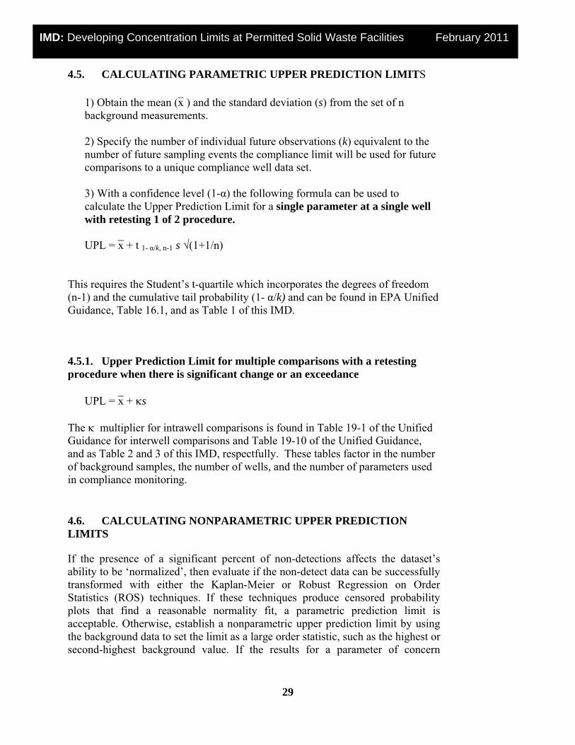
4.5. CALCULATING PARAMETRIC UPPER PREDICTION LIMITS 1) Obtain the mean (x̄ ) and the standard deviation (s) from the set of n background measurements. 2) Specify the number of individual future observations (k) equivalent to the number of future sampling events the compliance limit will be used for future comparisons to a unique compliance well data set. 3) With a confidence level (1-α) the following formula can be used to calculate the Upper Prediction Limit for a single parameter at a single well with retesting 1 of 2 procedure. UPL = x̄ + t 1- α/k, n-1 s √(1+1/n)

This requires the Student’s t-quartile which incorporates the degrees of freedom (n-1) and the cumulative tail probability (1- α/k) and can be found in EPA Unified Guidance, Table 16.1, and as Table 1 of this IMD.

4.5.1. Upper Prediction Limit for multiple comparisons with a retesting procedure when there is significant change or an exceedance

UPL = x̄ + κs

The κ multiplier for intrawell comparisons is found in Table 19-1 of the Unified Guidance for interwell comparisons and Table 19-10 of the Unified Guidance, and as Table 2 and 3 of this IMD, respectfully. These tables factor in the number of background samples, the number of wells, and the number of parameters used in compliance monitoring.

4.6. CALCULATING NONPARAMETRIC UPPER PREDICTION LIMITS If the presence of a significant percent of non-detections affects the dataset’s ability to be ‘normalized’, then evaluate if the non-detect data can be successfully transformed with either the Kaplan-Meier or Robust Regression on Order Statistics (ROS) techniques. If these techniques produce censored probability plots that find a reasonable normality fit, a parametric prediction limit is acceptable. Otherwise, establish a nonparametric upper prediction limit by using the background data to set the limit as a large order statistic, such as the highest or second-highest background value. If the results for a parameter of concern

29

30 30


contains all non-detect data, then construct a non-parametric prediction limit using the LOQ for that parameter.

It is important to know that using non-parametric prediction limits will require much more background data then normally needed. For example, 38 background samples are needed in order to predict two future samples with a 95% confidence. This is because we do not know the form of the underlying distribution of the non-parametric data.

The process for calculating an approximate non-parametric limit is as follows:

• Sort the background data by value/rank.

• Set the non-parametric upper prediction limit (UPL) equal to the largest or second-largest value (note: it is important to determine if any of the ranked data are outliers before conducting this step. Outliers should not be included in the dataset used to establish limits.)

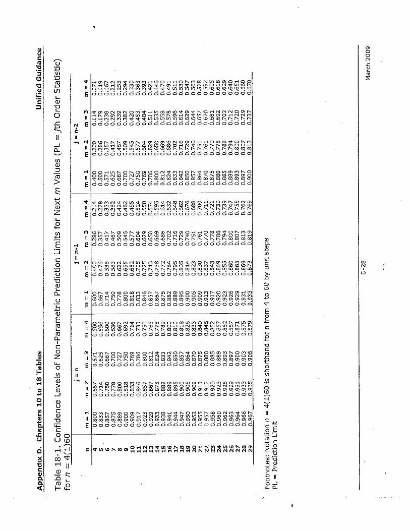
• Use Table 18-1 of the Unified Guidance (Table 4 of this IMD) o determine the confidence level (1-α) for predicting the next ‘m’ future compliance point samples.

• Compare each of the ‘m’ measurements to the UPL. Identify any significant exceedances.

• Because the risk of a false positive error driving a decision can be increased if the confidence limit falls below the target rate of 90-95%, the actual confidence level can be determined on a routine basis, using the following equation;

1-α = (j + m-1)* (j+m-2)…*(j+1)

.j

(n+m)*(n+m-1)…*(n+2)*(n+1) where n= sample size, j=rank of prediction limit value, and m=number of future samples to be compared to the limit

The above formula is appropriate for one constituent at a single compliance well. When multiple tests are required, determine the confidence level of the non-parametric UPL using Table 19.19 of the Unified Guidance (Table 5 of this IMD.) (note: be sure to include the 1 of 2 testing protocol.)

30

31 31


Chapter 5. Conducting Long-Term Compliance Monitoring The Department will approve a site-specific, long-term compliance monitoring program after background conditions are determined, a revised environmental monitoring plan (EMP) is approved, and concentration limits established. Compliance monitoring should include the collection and analysis of those parameters selected for concentration limits and other parameters that have been included in the approved EMP. Compliance monitoring should continue throughout the active life of the facility and the post-closure care period. As outlined in the permit, facilities will need to obtain the Department’s approval when there is a need to change the compliance-monitoring program.

5.1 PERIODIC REVIEW OF CONCENTRATION LIMIT VALUES

Every 5 years (at a minimum), DEQ staff should review the background groundwater quality data for facilities that used an inter-well statistical method of establishing concentration limits. This review should help determine if the existing concentration limits are still valid.

Similarly, staff should review those facilities that used an intra-well statistical method for establishing site-specific concentration limits. Once every five years (at a minimum), the facility groundwater quality data that do not exceed the approved concentration limits coupled with all appropriate historical data can be used to calculate new statistical limits.

These periods include both the permit renewal application and the 4-6 year Department review of any existing permit. These reviews and recalibration of limits improve the statistical power of the monitoring program by minimizing the frequency of false-positive and false-negative rates and decreasing result variances. Keeping these factors minimized can result in lower, statistically derived concentration limits.

5.2 EVIDENCE OF SIGNIFICANT CHANGE IN GROUNDWATER QUALITY

Evaluation of groundwater monitoring data continues during long-term compliance monitoring. This review should occur immediately after receipt of the results from the laboratory. Analytical results should be checked after every monitoring event to assess if the data meet QA/QC criteria. Such a review of the water quality data will determine if there is an exceedance of a concentration limit or an indication of a significant change of water quality.

31

32 32


A concentration limit exceedance would include the following:

• Parameter detected at a concentration above a permit-specific concentration limit (PSCL), concentration limit variance (CLV) or an action limit (AL), or

• Three or more parameters detected at a concentration above site-specific limits (SSL) in a specific monitoring location (if established).

The Groundwater Quality Protection rules (OAR 340-40) require re-sampling when monitoring indicates a significant increase (increase or decrease for pH). The rule does not define the term “significant increase (increase or decrease for pH)”. In order to minimize unnecessary and expensive re-sampling, the DEQ SW Program has used the following in permits as examples of a “significant change in water quality”:

• Quantification of a volatile organic compound (VOC), or other hazardous parameter, previously not detected during background groundwater quality monitoring, or

• A new exceedance of an OAR 340-40, Table 1, 2 or 3 reference or guidance level, unless the background groundwater quality also exceeds these numerical limits, or

• Exceeding any one federal primary drinking water standards (maximum contaminant levels [MCL]), established under the Safe Drinking Water Act, unless the background groundwater quality also exceeds these numerical limits, or

• Quantification of a compound at an order of magnitude higher than background.

Some permits direct the permittee to notify DEQ if the monitoring results identify either an exceedance of one or more concentration limit(s), or indicate a significant change in groundwater quality. Many of the SW permits require immediate verification sampling when an exceedance or a significant change of water quality occurs. Permittees should check with the DEQ Hydrogeologists if they suspect a significant change of water quality has occurred, to confirm the need for any re-sampling activity.

Re-sampling may not be required, if the significant change in groundwater quality was previously detected and the permittee has confirmed that to the Department in writing.

The assigned Solid Waste hydrogeologist should provide guidance to the permittee to evaluate their options for complying with Oregon’s Groundwater Quality Protection Rules (OAR 340-40.)

32

33 33


5.3 VERIFICATION RESAMPLING AND PRELIMINARY ASSESSMENTS

If re-sampling results confirm the exceedance or significant change in groundwater quality, and if the change in groundwater quality cannot be explained after reviewing the original laboratory data, QA/QC reports and the re-sampling results, many of the permits direct the permittee to:

• Notify the Department in writing of the change in groundwater quality within 10 days of receipt of the laboratory results. The notification should identify the monitoring well(s) and associated parameter(s).

• If this is a Subtitle D landfill, perform assessment monitoring at the affected compliance well(s) within 90 days of confirmation of an exceedance. Assessment monitoring will not be required if there is a valid demonstration that the change in water quality is not attributable to landfill operations.

• Submit a preliminary assessment (PA) work plan to the Department within 30 days of confirmation to address the exceedance of one PSCL or a CLV of a previously undetected VOC, or other hazardous parameter is confirmed with resampling. The Department may approve an alternate schedule for submission of a PA work plan.

• If an AL or three or more SSLs are exceeded, then the permittee should submit an informal preliminary assessment (IPA) work plan to the DEQ SW Program within 30 days of confirmation, unless another schedule is approved by the Department.

No further action is needed if the resampling did not confirm the significant change. The permittee should resume long-term compliance monitoring. The original anomalous result should be flagged in the statistical database and replaced with the resample results when statistics are generated (per the 1 of 2 re-sampling protocol). The subsequent annual environmental monitoring report should discuss this event.

The inclusion of anomalies and systematic error values in the database used for statistical evaluations could cause misinterpretation of the database and result in high false positive (an indication of a release when none exists) or false negative (concluding there is no release when one exists) conclusions.

33

34 34


References

Cravy, TD., McIassac, P, and Gibbons, R.D., 1990. Evaluation of organic indicator para‐ meters using an Appendix VII/IX Database: presented at Waste Tech ’90 Landfill Technology: Back to Basics. San Francisco, CA. Gibbons. R.D., 1994. Intra‐well statistical methods for ground‐water monitoring at waste disposal sites. Chicago. July 25. Gibbons, R.D., 1996. Statistical methods for groundwater monitoring at WMX Columbia Ridge Landfill & Recycling Center. March 1. Hem, J. D., 1992. Study and Interpretation of the Chemical Characteristics of Natural Water. U.S. Geological Survey Water‐Supply Paper 2254. Plumb, R.H., 1991. The occurrence of Appendix IX organic constituents in disposal site groundwater. GWMR, 11(2):157‐164.

US EPA 1992. Statistical analysis of ground‐water monitoring data at RCRA facilities. Addendum to interim final guidance document. July.

US EPA 1996. Soil Screening Guidance: Users Guide. July.

US EPA 2009. Statistical analysis of groundwater monitoring data at RCRA facilities: Unified Guidance. March.

34

35 35


Appendix A: Parameter Groups – Solid Waste Facilities Group 1a: Field indicators

The following parameters comprise the field indicators parameter group:

Elevation of water level Specific Conductance pH Dissolved Oxygen Temperature Eh

These parameters must be measured in the field at the time samples are collected, either down-hole in situ, in a flow-through cell, or immediately following sample recovery, with instruments calibrated to relevant standards

Group 1b: Leachate indicators

The following parameters comprise the laboratory indicators parameter group Hardness (as CaCO3) Total Dissolved Solids (TDS) Total Alkalinity (as CaCO3) Total Suspended Solids (TSS) Total Organic Carbon (TOC) Chemical Oxygen Demand (COD) Specific Conductance (lab) pH (lab) Tannin/Lignin (woodwaste)

Sample handling, preservation, and analysis are determined by requirements for each individual analyte. Group 2a: Common anions and cations

The following parameters comprise the common anions and cations parameter group: Calcium (Ca) Manganese (Mn) Sulfate (SO4) Magnesium (Mg) Ammonia (NH3) Chloride (Cl) Sodium (Na) Carbonate (CO3) Nitrate (NO3) Potassium (K) Silica (SiO2) Bicarbonate (HCO3) Iron (Fe) Ammonium (NH4) Fluoride (F)

Dissolved concentrations must be measured. Samples must be field-filtered and field-preserved. Results reported in mg/L and meq/L.

Group 2b: Trace metals

The following parameters comprise the trace metals parameter group: Antimony (Sb) Chromium (Cr) Selenium (Se) Arsenic (As) Cobalt (Co) Silver (Ag) Barium (Ba) Copper (Cu) Thallium (Tl) Beryllium (Be) Lead (Pb) Vanadium (V) Cadmium (Cd) Nickel (Ni) Zinc (Zn)

35

36 36


If the Total Suspended Solids concentration is less than or equal to 100.0 mg/L in the sample then analyze metals for total concentrations (unfiltered). If the Total Suspended Solids concentration is greater than 100.0 mg/L in the sample then analyze metals for both dissolved (filtered) and total concentrations (unfiltered). Group 3: Volatile organic constituents Analysis for all compounds detectable by an appropriate EPA Method, including a library search to identify any unknown compounds present. EPA Method 8260 comprises the volatile organic constituent’ parameter group.

36

37 37 IMD: Developing Concentration Limits at Permitted Solid Waste Facilities February 2011

Appendix B – Boxplot

In descriptive statistics, a box plot or boxplot (also known as a box-and-whisker diagram or plot) is a convenient way of graphically depicting groups of numerical data through their five-number summaries (the smallest observation (sample minimum), lower quartile (Q1), median (Q2), upper quartile (Q3), and largest observation (sample maximum). A boxplot may also indicate which observations, if any, might be considered outliers.

Source: http://upload.wikimedia.org/wikipedia/commons/8/89/Boxplot_vs_PDF.png

37

http://en.wikipedia.org/wiki/Descriptive_statistics

http://en.wikipedia.org/wiki/Five-number_summary

http://en.wikipedia.org/wiki/Sample_minimum

http://en.wikipedia.org/wiki/Sample_minimum

http://en.wikipedia.org/wiki/Quartile

http://en.wikipedia.org/wiki/Median

http://en.wikipedia.org/wiki/Quartile

http://en.wikipedia.org/wiki/Sample_maximum

http://en.wikipedia.org/wiki/Outlier

38 38


Appendix C

Shapiro-Wilk Example

The Shapiro-Wilk test is the most reliable test of-normality/non-normality for a sample size of 3-50, and is suitable for use on un-altered data or on transformed data. The test will compute a Shapiro-Wilk statistic (SW) which is then compared to an α- critical level point. If the test statistic SW is greater than the α-critical level, there is significant evidence of normal distribution. If the test statistic SW is less than the α-critical level, there is significant evidence of non-normal distribution.

Shapiro-Wilk Example: How to compute a SW for a dataset with 20 samples from a single or pooled background well(s)

i

Xi

ranked

concentration

lowest to highest

X(n-i +1)

Column 2

in reverse

order

X(n-I +1) – Xi

Column 3-

Column 2

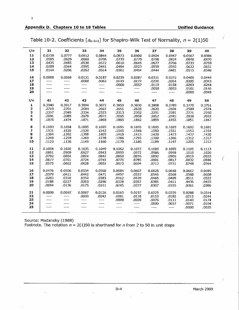
a(n-i+1)

from Table

10.2 in EPA

U.G.

bi

Column 4

multiplied by

Column 5 1 3.4 321 317.6 0.4734 150.35 2 4.0 271 267.0 0.3211 85.73 3 4.5 255 250.5 0.2565 64.25 4 5.6 150 144.4 0.2085 30.11 5 6.7 126 119.3 0.1686 20.11 6 10.0 120 110.0 0.1334 14.67 7 21 102 81.0 0.1013 8.21 8 33 98 65.0 0.0711 4.62 9 35 80 55.0 0.0422 2.32 10 63 65 2.0 0.0140 0.03 11 65 63 -2.0 12 80 35 -55.0 b = 380.40 13 98 33 -65.0 14 102 21 -81.0 15 120 10.0 -110.0 16 126 6.7 -119.3 17 150 5.6 -144.4 18 255 4.5 -250.3 19 271 4.0 -267.0 20 321 3.4 -317.6

38

39 39


SW = [ b/ (s)(√(n-1) ]2 [note: s = standard deviation]

SW = [ 380.4/ (95.83)(√(19) ]2

SW = 0.8293 From Table 10.3 of the EPA Unified Guidance, the α- critical level for 0.01 with 20 samples is 0.868. The calculated SW of 0.8298 is less than the α- critical level, thus the data set shows significant evidence of non-normality. The data can be transformed (log/ln) and normality rechecked before proceeding with a nonparametric procedure. Unified Guidance Tables that are important for the Shapiro-Wilk calculations are included in Table 6 of this IMD. Note: for data sets of n<10, α- critical level = 0.10; for datasets of 10<n<20, α- critical level = 0.05; for datasets greater than 20 and <50, α- critical level = 0.01. When n > 50, use the Shapiro-Francia test of normality.

39

40 40


Appendix D

Non Parametric Comparisons with Pooled Background Data Example

Sample Event

Concentration of a single parameter in pooled background wells (ug/L)

BG MW-1 BG MW-2 BG MW-3

Concentration in Compliance

Well CW-1 (ug/L)

1 7 <5 <5

2 6.5 <5 <5

3 <5 8 10.5 8

4 12 <5 <5 14

5 <5 9 <5 <5

6 6 10 9 7.5

Ranking the background data, n=18, the maximum value would be 12 ug/L.

The non-parametric UPL is set at 12.

Comparing the compliance well data to the UPL, one can see that in event 4, the value in CW-1 of 14 ug/L exceeds the UPL.

To better assess this ‘exceedance’, compute the confidence level and the false positive rate associates with the UPL Use the following constants:

o n = 18

o m = number of CW measurements (comparisons) = 4

o Confidence level = n/(n+m) = 18/22 = 82% 0r 0.82

o False positive rate (Type 1 error) = 1-0.82 = 18%

o The test is significant at α = 0.18.

In this example, there is an approximate one in five chance that the exceedance is falsely verified. Additional background data can help to lower the false positive rate.

40

41 41

41


Attachment 1

Associated Tables from US EPA Unified Guidance Document, 2009

Date post:	19-Jan-2020
Category:	Documents
Upload:	others
View:	7 times
Download:	0 times

Internal Management Directive Library/IMD-DevConLimitsFacilities.pdfIMD: Developing Concentration...

Documents