HAL Id: hal-00148529https://hal.archives-ouvertes.fr/hal-00148529v3

Submitted on 18 Dec 2007

HAL is a multi-disciplinary open accessarchive for the deposit and dissemination of sci-entific research documents, whether they are pub-lished or not. The documents may come fromteaching and research institutions in France orabroad, or from public or private research centers.

L’archive ouverte pluridisciplinaire HAL, estdestinée au dépôt et à la diffusion de documentsscientifiques de niveau recherche, publiés ou non,émanant des établissements d’enseignement et derecherche français ou étrangers, des laboratoirespublics ou privés.

Internal states of model isotropic granular packings. I.Assembling process, geometry and contact networks.

Ivana Agnolin, Jean-Noël Roux

To cite this version:Ivana Agnolin, Jean-Noël Roux. Internal states of model isotropic granular packings. I. Assemblingprocess, geometry and contact networks.. Physical Review E : Statistical, Nonlinear, and Soft MatterPhysics, American Physical Society, 2007, 76 (6), pp.061302. <10.1103/PhysRevE.76.061302>. <hal-00148529v3>

hal-

0014

8529

, ver

sion

3 -

18

Dec

200

7Internal states of model isotropic granular packings.

I. Assembling process, geometry and contact networks.

Ivana Agnolin∗ and Jean-Noel Roux†

Laboratoire des Materiaux et des Structures du Genie Civil‡, Institut Navier,

2 allee Kepler, Cite Descartes, 77420 Champs-sur-Marne, France

(Dated: December 18, 2007)

This is the first paper of a series of three, in which we report on numerical simulation studiesof geometric and mechanical properties of static assemblies of spherical beads under an isotropicpressure. The influence of various assembling processes on packing microstructures is investigated. Itis accurately checked that frictionless systems assemble in the unique random close packing (RCP)state in the low pressure limit if the compression process is fast enough, higher solid fractionscorresponding to more ordered configurations with traces of crystallization. Specific propertiesdirectly related to isostaticity of the force-carrying structure in the rigid limit are discussed. Withfrictional grains, different preparation procedures result in quite different inner structures thatcannot be classified by the sole density. If partly or completely lubricated they will assemble likefrictionless ones, approaching the RCP solid fraction ΦRCP ≃ 0.639 with a high coordination number:z∗ ≃ 6 on the force-carrying backbone. If compressed with a realistic coefficient of friction µ = 0.3packings stabilize in a loose state with Φ ≃ 0.593 and z∗ ≃ 4.5. And, more surprisingly, an idealized“vibration” procedure, which maintains an agitated, collisional regime up to high densities resultsin equally small values of z∗ while Φ is close to the maximum value ΦRCP. Low coordinationpackings have a large proportion (>10%) of rattlers – grains carrying no force – the effect of whichshould be accounted for on studying position correlations, and also contain a small proportion oflocalized “floppy modes” associated with divalent grains. Low pressure states of frictional packingsretain a finite level of force indeterminacy even when assembled with the slowest compression ratessimulated, except in the case when the friction coefficient tends to infinity. Different microstructuresare characterized in terms of near neighbor correlations on various scales, and some comparisons withavailable laboratory data are reported, although values of contact coordination numbers apparentlyremain experimentally inaccessible.

PACS numbers: 45.70.-n, 83.80.Fg, 46.65.+g, 62.20.Fe

I. INTRODUCTION

A. Context and motivations

The mechanical properties of solidlike granular pack-ings and their microscopic, grain-level origins are an ac-tive field of research in material science and condensed-matter physics [1, 2, 3]. Motivations are practical, origi-nated in soil mechanics and material processing, as wellas theoretical, as general approaches to the rheology ofdifferent physical systems made of particle assemblies outof thermal equilibrium [4] are attempted.

The packing of equal-sized spherical balls is a simplemodel for which there is a long tradition of geometric

characterization studies. Packings are usually classifiedaccording to their density or solid volume fraction Φ, andthe frequency of occurrence of some local patterns. Di-rect observation of packing microstructure is difficult, al-though it has recently benefitted from powerful imaging

∗Present address: Geoforschungszentrum, Haus D, Telegrafenberg,

D-14473 Potsdam, Germany‡LMSGC is a joint laboratory depending on Laboratoire Central

des Ponts et Chaussees, Ecole Nationale des Ponts et Chaussees

and Centre National de la Recherche Scientifique†Electronic address: jean-noel.roux@lcpc.fr

techniques [5, 6, 7]. The concept of random close pack-ing (RCP), is often invoked [8, 9], although some authorscriticized it as ill-defined [10]. It corresponds to the com-mon observation that bead packings without any traceof crystalline order do not exceed a maximum density,ΦRCP , slightly below 0.64 [8].

Mechanical studies in the laboratory have been per-formed on granular materials for decades in the realmof soil mechanics, and the importance of packing frac-tion Φ on the rheological behavior has long been rec-ognized [1, 11, 12, 13]. The anisotropy of the packingmicrostructure, due to the assembling process, has alsobeen investigated [14, 15], and shown to influence thestress-strain behavior of test samples [16], as well as thestress field and the response to perturbations of gravity-stabilized sandpiles or granular layers [17].

Discrete numerical simulation [18] proved a valuabletool to investigate the internal state of packings, as itis able to reproduce mechanical behaviors, and to iden-tify relevant variables other than Φ, such as coordinationnumber and fabric (or distribution of contact orienta-tions) [19, 20, 21, 22, 23]. In the case of sphere packings,simulations have been used to characterize the geometryof gravity-deposited systems [24, 25] or oedometricallycompressed ones [26], to investigate the quasistatic, hys-teretic stress-strain dependence in solid packings [27, 28],and their pressure-dependent elastic moduli in a com-

2

pression experiment [29, 30].However, in spite of recent progress, quite a few ba-

sic questions remain unresolved. It is not obvious howclosely the samples used in numerical simulations actu-ally resemble laboratory ones, for which density is oftenthe only available state parameter. Both simulations andexperiments resort to certain preparation procedures toassemble granular packings, which, although their influ-ence is recognized as important, are seldom studied, oreven specified. One method to produce dense packingsin simulations is to set the coefficient of intergranularfriction to zero [26, 27] or to a low value [28] in theassembling stage, while a granular gas gets compactedand equilibrated under pressure. On keeping friction-less contacts, this results, in the limit of low confin-ing stress, in dense systems with rather specific proper-ties [30, 31], related to isostaticity and potential energyminimization [32]. Examples of traditional proceduresin soil mechanics are rain deposition under gravity, alsoknown as air pluviation (which produces homogeneousstates if grain flow rate and height of free fall [33] aremaintained constant) and layerwise deposition and dryor moist tamping. Those two methods were observed toproduce, in the case of loose sands, different structuresfor the same packing density [34]. Densely packed parti-cle assemblies can also be obtained in the laboratory byvibration, or application of repeated “taps” [35, 36] to aloose deposit. How close are dense experimental spherepackings to model configurations obtained on simulatingfrictionless particles ? How do micromechanical parame-ters influence the packing structure ? Is the low pressurelimit singular in laboratory grain packings and in whatsense ?

B. Outline of the present study

The present paper provides some answers to such ques-tions, from numerical simulations in the simple caseof isotropically assembled and compressed homogeneouspackings of spherical particles. It is the first one of aseries of three, and deals with the geometric characteri-zation of low pressure isotropic states assembled by dif-ferent procedures, both without and with intergranularfriction. The other two, hereafter referred to as papersII [37] and III [38], respectively investigate the effectsof compressions and pressure cycles, and the elastic re-sponse of the different numerical packings, with compar-isons to experimental results. Although mechanical as-pects are hardly dealt with in the present paper, we insistthat geometry and mechanics are strongly and mutuallyrelated. We focus here on the variability of the coordi-nation numbers, which will prove important for mechan-ical response properties of granular packings, and showthat equilibrated packs of identical beads can have a rel-atively large numbers of “rattler” grains, which do notparticipate in force transmission. We investigate the de-pendence of initial states on the assembling procedure,

both with and without friction. We study the effectsof procedures designed to produce dense states (close toRCP), and we characterize the geometry of such stateson different scales.

It should be emphasized that we do not claim here tomimic experimental assembling procedures very closely.Rather, we investigate the results of several prepara-tion methods, which are computationnally convenient,maintain isotropy, and produce equilibrated samples withrather different characteristics. Those methods neverthe-less share some important features with laboratory pro-cedures, and we shall argue that the resulting states areplausible models for experimental samples.

The numerical model and the simulation procedures(geometric and mechanical parameters, contact law,boundary conditions) are presented in Section II, wheresome basic definitions and mechanical properties per-taining to granular packs are also presented or recalled.Part III discusses the properties of frictionless packings,and introduces several characterization approaches usedin the general case as well. Section IV then describes dif-ferent assembling procedures of frictional packings andthe resulting microstructures. Section V discusses per-spectives to the present study, some of which are pur-sued in papers II and III of the series. Appendices dealwith technical issues, and also present a more detailedcomparison with some experimental data.

This being a long paper, it might be helpful to specifywhich parts can be read independently. On first goingthrough the paper, the reader might skip Section III D,dealing with a rather specific issue. The properties statedor recalled in Section II C are used to discuss stability is-sues and isostatic values of coordination numbers, butthey can also be overlooked in a first approach. Finally,Section IV can be read independently from Section III,apart from the explanations about equilibrium conditions(in paragraph III B 2) and the treatment of rattlers (para-graph III E 1). Sections III and IV both have conclusivesubsections which summarize the essential results.

II. MODEL, NUMERICAL PROCEDURES,BASIC DEFINITIONS

A. Intergranular forces

We consider spherical beads of diameter a (the valueof which, as we ignore gravity, will prove irrelevant), in-teracting in their contacts by the Hertz law, relating thenormal force N to the elastic normal deflection h as :

N =E√

a

3h3/2. (1)

In Eqn. 1, we introduced the notation

E =E

1 − ν2,

3

E is the Young modulus of the beads, and ν the Poissonratio. For spheres, h, the elastic deflection of the contact,is simply the distance of approach of the centers beyondthe first contact. The normal stiffness KN of the contactis defined as the rate of change of the force with normaldisplacement:

KN =dN

dh=

E√

a

2h1/2 =

31/3

2E2/3a1/3N1/3 (2)

Although many geometric features of particle packingsdo not depend on the details of the model for contactelasticity, and could be observed as well with a simpler,unilateral elastic model, it is necessary to implement suit-able non-linear contact models to deal with the mechan-ical properties in papers II and III [37, 38]. Tangentialelasticity and friction in contacts are appropriately de-scribed by the Cattaneo-Mindlin-Deresiewicz laws [39],which we implement in a simplified form, as used e.g., inrefs. [29, 41]: the tangential stiffness KT relating, in theelastic regime, the increment of tangential reaction dT tothe relative tangential displacement increment duT is afunction of h (or N) alone (i.e., it is kept constant, equalto its value for T = 0):

dT = KT duT , with

KT =2 − 2ν

2 − νKN =

1 − ν

2 − νE√

ah1/2(3)

To enforce the Coulomb condition with friction coeffi-cient µ, T has to be projected back onto the circle ofradius µN in the tangential plane whenever the incre-ment given by eqn. 3 would cause its magnitude to ex-ceed this limit. Moreover, when N decreases to N − δN ,T is scaled down to the value it would have had if Nhad constantly been equal to N − δN in the past. Itis not scaled up when N increases. Such a procedure,suggested e.g., in [40], avoids spurious increases of elas-tic energy for certain loading histories. More details aregiven in Appendix A.

Finally, tangential contact forces have to follow the ma-terial motion. Their magnitudes are assumed here not tobe affected by rolling (i.e., rotation about a tangentialaxis) or pivoting (i.e., rotation about the normal axis),while their direction rotates with the normal vector dueto rolling, and spins around it with the average spinningrate of the two spheres (to ensure objectivity). The cor-responding equations are given in Appendix B.

In addition to the contact forces specified above, weintroduce viscous ones, which oppose the normal rela-tive displacements (we use the convention that positivenormal forces are repulsive):

Nv = α(h)h (4)

The damping coefficient α depends on h, and we chooseits value as a fixed fraction ζ of the critical dampingcoefficient of the normal (linear) spring of stiffness KN (h)(as given by (2)) joining two beads of mass m:

α(h) = ζ√

2mKN(h). (5)

From (2), α is thus proportional to h1/4, or to N1/6.The same damping law was used in [41]. Admittedly,the dissipation given by (4)-(5) has little physical justifi-cation, and is rather motivated by computational conve-nience. We shall therefore assess the influence of ζ on thenumerical results. The present study being focussed onstatics, we generally use a strong dissipation, ζ = 0.98,to approach equilibrium faster. This particular value isadmittedly rather arbitrary: the initial motivation forchoosing ζ < 1 is the computational inefficiency of over-damped contacts with ζ > 1 in the case of linear contact

elasticity. Yet we did not check whether values of 1 oreven higher would cause any problem with Hertzian con-

tacts. In the linear case, the restitution coefficient in abinary collision varies as a very fastly decreasing func-tion of ζ, and changes of ζ in the range between 0.7 and1 have virtually no detectable effect.

We do not introduce any tangential viscous force, andimpose the Coulomb inequality to elastic force compo-nents only. We choose the elastic parameters E = 70 GPaand ν = 0.3, suitable for glass beads, and the friction co-efficient is attributed a moderate, plausible value µ = 0.3.These choices are motivated by comparisons to experi-mental measurements of elastic moduli, to be carried outin paper III [38].

B. Boundary conditions and stress control

The numerical results presented below were obtainedon samples of n = 4000 beads, enclosed in a cubic orparallelipipedic cell with periodic boundary conditions.

It is often in our opinion more convenient to use pres-sure (or stress) than density (or strain) as a control pa-rameter (a point we discuss below in Section III). Wetherefore use a stress-controlled procedure in our sim-ulations, which is adapted from the Parrinello-Rahmanmolecular dynamics (MD) scheme [42]. The simulationcell has a rectangular parallelipipedic shape with lengthsLα parallel to coordinate axes α (1 ≤ α ≤ 3). Lα valuesmight vary, so that the system has 6N +3 configurationaldegrees of freedom,which are the positions and orienta-tions of the N particles and lengths Lα. Ω = L1L2L3

denotes the sample volume. We seek equilibrium stateswith set values (Σα)1≤α≤3 of all three principal stressesσαα. We use the convention that compressive stresses arepositive.

It is convenient to write position vectors ri, defining asquare 3 × 3 matrix with Lα’s on the diagonal, as

(1 ≤ i ≤ N) ri = L · si,

si denoting corresponding vectors in a cubic box of unitedge length. In addition to particle angular and linearvelocities, which read

(1 ≤ i ≤ N) vi = L · si + L · si,

one should evaluate time derivatives Li. Equations ofmotion are written for particles in the standard form,

4

i.e., (Fi denoting the total force exerted on grain i)

(1 ≤ i ≤ N) misi = L−1 · Fi, (6)

and the usual equation for angular momentum. Mean-while, lengths Lα satisfy the following equation of mo-tion, in which rij is the vector joining the center of i tothe center of j, subject to the usual nearest image con-vention of periodic boundary conditions:

MLα =1

Lα

L2α

∑

i

mi

(

s(α)i

)2

+∑

i<j

F(α)ij r

(α)ij

− Ω

LαΣα.

(7)

Within square brackets on the right-hand side of Eqn. 7,one recognizes the familiar formula [19, 43, 44] for Ωσαα,σ being the average stress in the sample:

σαβ =1

Ω

∑

i

mivαi vβ

i +∑

i<j

F(α)ij r

(α)ij

(8)

All three diagonal stress components should thus equatethe prescribed values Σα at equilibrium. The accelerationterm will cause the cell to expand in the correspondingdirection if the stress is too high, and to shrink if it istoo low. Eqn. 7 involves a generalized mass M associatedwith the changes of shape of the simulation cell. M is setto a value of the order of the total mass of all particles inthe sample. This choice was observed to result in collec-tive degrees of freedom Lα approaching their equilibriumvalues under prescribed stress Σ somewhat more slowly(but not exceedingly so) than (rescaled) positions s.

The original Parrinello-Rahman method was designedfor conservative molecular systems, in such a way thatthe set of equations is cast in Lagrangian form. Thisimplies in particular additional terms in (6), involving

L. Such terms were observed to have a negligible influ-ence on our calculations and were consequently omitted.Granular materials are dissipative, and energy conserva-tion is not an issue (except for some elastic properties, seepaper III [38]). Further discussion of the stress-controlledmethod is provided in Appendix C.

Equations (6) and (7), with global degrees of free-dom Lα slower than particle positions, lead to dynam-ics similar to those of a commonly used procedure ingranular simulation [45]. This method consists in re-peatedly changing the dimensions of the cell by verysmall amounts, then computing the motion of the grainsfor some interval of time. A “servo mechanism” can beused to impose stresses rather than strains [30]. Our ap-proach might represent a simplification, as it avoids sucha two-stage procedure. It should be kept in mind thatwe restricted our use of equation (7) to situations whenchanges in the dimensions of the simulation cell are veryslow and gradual. The perturbation introduced in themotion of the grains, in comparison to the more familiarcase of a fixed container, is very small.

C. Rigidity and stiffness matrices

We introduce here the appropriate formalism and statethe relevant properties of static contact networks. It isimplied throughout this section that small displacementsabout an equilibrium configurations are dealt with to firstorder (as an infinitesimal motion, i.e. just like veloci-ties), and related to small increments of applied forces,moments and stresses. In the following we shall exploit

the definitions of stiffness matrices K(1) (Eqn. 18) and

K(2) to discuss stability properties of packings. The

corrections to the degree of force indeterminacy due tofree mechanism motions, as expressed by relations (19)or (20), will also be used.

The properties are stated in a suitable form to the peri-odic boundary conditions with controlled diagonal stresscomponents, as used in our numerical study.

1. Definition of stiffness matrix

We consider a given configuration with bead centerpositions (ri, 1 ≤ i ≤ n) and orientations (θi, 1 ≤ i ≤ n),and cell dimensions (Lα, 1 ≤ α ≤ 3). The grain centerdisplacements (ui)1≤i≤n are conveniently written as

ui = ui − ǫ · ri,

with a set of displacements ui satisfying periodic bound-ary conditions in the cell with the current dimensions,and the elements of the diagonal strain matrix ǫ expressthe relative shrinking deformation along each direction,ǫα = −∆Lα/Lα. Gathering all coordinates of particle(periodic) displacements and rotation increments, alongwith strain parameters, one defines a displacement vector

in a space with dimension equal to the number of degreesof freedom Nf = 6n + 3,

U = ((ui, ∆θi)1≤i≤n, (ǫα)1≤α≤3) . (9)

Let Nc denote the number of intergranular contacts. Inevery contacting pair i-j, we arbitrarily choose a “first”grain i and a “second” one j. The normal unit vectornij points from i to j (along the line joining centers forspheres). The relative displacement δuij is defined forspherical grains with radius R as

δuij = ui + δθi × Rnij − uj + δθj × Rnij + ǫ · rij , (10)

in which rij is the vector pointing from the center ofthe first sphere i to the nearest image of the center ofthe second one j. The normal part δuN

ij of δuij is theincrement of normal deflection hij in the contact. (10)defines a 3Nc × Nf matrix G which transforms U intothe 3Nc-dimensional vector of relative displacements atcontacts δu:

δu = G · U (11)

5

In agreement with the literature on rigidity theory offrameworks [46] (−G is termed normalized rigidity ma-trix in that reference), we call G the rigidity matrix.

In each contact a force Fij is transmitted from i to j,which is split into its normal and tangential componentsas Fij = Nijnij + Tij . The static contact law (withoutviscous terms) expressed in Eqns. (1), (3), with the condi-tions stated in Section II A, relates the 3Nc-dimensionalcontact force increment vector ∆f , formed with the val-ues ∆Nij , ∆Tij of the normal and tangential parts of allcontact force increments, to δu:

∆f = K · δu. (12)

This defines the (3Nc×3Nc) matrix of contact stiffnessesK. K is block diagonal (it does not couple different con-tacts), and is conveniently written on using coordinateswith nij as the first basis unit vector. In simple cases the3 × 3 block of K corresponding to contact i, j, K

ijis di-

agonal itself and contains stiffnesses KN(hij) and (twicein 3 dimensions) KT (hij) as given by (2) and (3):

Kij

=

KN(hij) 0 00 KT (hij) 00 0 KT (hij)

. (13)

More complicated non-diagonal forms of Kij

, which actu-

ally depend on the direction of the increments of relativesdisplacements in the contact, are found if friction is fullymobilized (which does not happen in well-equilibratedconfigurations), or corresponding to those small motionsreducing the normal contact force. The effects of suchterms is small, with our choice of parameters, and is dis-cussed in paper III [38].

External forces Fi and moments Γi (at the center) ap-plied to the grains, and diagonal Cauchy stress compo-nents Σα can be gathered in one Nf -dimensional load

vector Fext:

Fext = ((Fi,Γi)1≤i≤n, (ΩΣα)1≤α≤3) , (14)

chosen such that the work in a small motion is equal toF

ext ·U. The equilibrium equations – the statements thatcontact forces f balance load F

ext – is simply written withthe tranposed rigidity matrix, as

Fext = T

G · f . (15)

This is of course easily checked on writing down all forceand moment coordinates, as well as the equilibrium formof stresses:

ΩΣα =∑

i<j

Fαijr

αij . (16)

As an example, matrices G and TG were written down

in [47] in the simple case of one mobile disk with 2 con-tacts with fixed objects in 2 dimensions, the authors re-ferring to − T

G as the “contact matrix”. The same defi-nitions and matrices are used in [48] in the more generalcase of a packing of disks.

Returning to the case of small displacements associatedwith a load increment ∆F

ext, one may write, to firstorder in U,

∆Fext = K ·U, (17)

with a total stiffness matrix K, comprising two parts,

K(1) and K

(2), which we shall respectively refer to as

the constitutive and geometric stiffness matrices. K(1)

results from Eqns. 11, 12 and 15:

K(1) = T

G · K · G. (18)

K(2) is due to the change of the geometry of the pack-

ing. Its elements (see Appendix B), relatively to to their

counterparts in K(1), are of order F/KNR ∼ h/R, and

therefore considerably smaller in all practical cases. Theconstitutive stiffness matrix is also called “dynamical ma-trix” [31, 41]. One advantage of decomposition (18) is toseparate out the effects of the contact constitutive law,contained in K and those of the contact network, con-tained in G. G is sensitive in general to the orientationsof normal unit vectors nij and to the “branch vectors”joining the grain centers to contact positions – which re-

duce to Rnij for spheres of radius R. K(2), on the other

hand, unlike G, is sensitive to the curvature of grain sur-faces at the contact point [49, 50].

2. Properties of the rigidity matrix

To the rigidity matrix are associated the concepts(familiar in structural mechanics) of force and velocity(or displacement) indeterminacy, of relative displacementcompatibility and of static admissibility of contact forces.Definitions and properties stated in [32] for frictionlessgrains, straightforwardly generalize to packings with fric-tion.

The degree of displacement indeterminacy (also calleddegree of hypostaticity [32]) is the dimension k of thekernel of G, the elements of which are displacements vec-tors U which do not create relative displacements in thecontacts: δu = 0. Such displacements are termed (first-order) mechanisms. Depending on boundary conditions,a grain packing might have a small number k0 of “triv-ial” mechanisms, for which the whole system moves asone rigid body. In our case, attributing common valuesof u to all grains gives k0 = 3 independent global rigidmotions.

The degree of force indeterminacy h (also called degreeof hyperstaticity [32]) is the dimension of the kernel ofTG, or the number of independent self-balanced contact

force vectors. If the coordinates of f are regarded asthe unknowns in system of equations (15), and if F

ext

is supportable, then there exists a whole h-dimensionalaffine space of solutions.

From elementary theorems in linear algebra one de-duces a general relation between h and k [32]

Nf + h = 3Nc + k. (19)

6

An isostatic packing is defined as one devoid of forceand velocity indeterminacy (apart from trivial mecha-nisms). Excluding trivial mechanisms (thus reducing Nf

to Nf − k0), and loads that are not orthogonal to them,one then has a square, invertible rigidity matrix. Toany load corresponds a unique set of equilibrium contactforces. To any vector of relative contact displacementscorresponds a unique displacement vector.

With frictionless objects, in which contacts only carrynormal forces, it is appropriate to use Nc-dimensionalcontact force and relative displacement vectors, contain-ing only normal components, and to define the rigiditymatrix accordingly [32]. Then (19) should be written as

Nf + h = Nc + k. (20)

In the case of frictionless spherical particles, all rotationsare mechanisms, hence a contribution of 3 to k. Thusone may in addition ignore all rotations, and subtract3n both from Nf and from k, so that (20) is still valid.In such a case, the rigidity matrix coincides (up to asign convention and normalization of its elements) withthe one introduced in central-force networks, trusses andtensegrity structures [51]. Donev et al., in a recent pub-lication on sphere packings [52], call rigidity matrix whatwe defined as its transpose T

G.

D. Control parameters

The geometry and the mechanical properties of spherepackings under given pressure P depends on a small setof control parameters, which can be conveniently definedin dimensionless form [23, 53].

Such parameters include friction coefficient µ and vis-cous dissipation parameter ζ, which were introduced inSec. II A.

The elastic contact law introduces a dimensionless

stiffness parameter κ, which we define as:

κ =

(

E

P

)2/3

. (21)

Note that κ does not depend on bead diameter a. Underpressure P , the typical force in a contact is of order Pa2.It corresponds to a normal deflection h such that Pa2 ∼E√

ah3/2 due to the Hertz law (1). Therefore, κ setsthe scale of the typical normal deflection h in Hertziancontacts, as h/a ∼ 1/κ.

In the case of monodisperse sphere packings in equi-librium in uniform state of stress σ, pressure P = trσ/3is directly related to the average normal force 〈N〉. Letus denote as Φ the solid fraction and z the coordinationnumber (z = 2Nc/n). As a simple consequence of theclassical formula for stresses recalled in Sec. II B (Eqn. 8in the static case, or Eqn. 16), one has, neglecting contactdeflections before diameter a,

P =zΦ〈N〉

πa2, (22)

whence an exact relation between P and contact deflec-tions:

〈h3/2〉a3/2

=π

zΦκ3/2.

The limit of rigid grains is approached as κ → ∞. κcan reach very high values for samples under their ownweight, but most laboratory results correspond to levelsof confining pressure in the 100 kPa range. Experimentaldata on the mechanical properties of granular materialsin quasistatic conditions below a few tens of kPa are veryscarce (see, however, [54] and [55]). This is motivated byengineering applications (100 kPa is the pressure below afew meters of earth), and this also results from difficultieswith low confining stresses. Below this pressure range,stress fields are no longer uniform, due to the influence ofthe sample weight, and measurements are difficult (e.g.,elastic waves of measurable amplitude are very stronglydamped).

We set the lowest pressure level for our simulation ofglass beads to 1 kPa or 10 kPa, which corresponds toκ ≃ 181000 and κ ≃ 39000. Such values, as we shallcheck, are high enough for some characteristic proper-ties of rigid sphere packings to be approached with goodaccuracy. Upon increasing P , the entire experimentalpressure range will be explored in the two companionpapers [37, 38].

Another parameter associated with contact elasticityis the ratio of tangential to normal stiffnesses (constantin our model), related to the Poisson ratio of the materialthe grains are made of. Although we did not investigatethe role of this parameter, several numerical studies [41,56] showed its influence on global properties to be verysmall.

The “mass” M of the global degrees of freedom is cho-sen to ensure slow and gradual changes in cell dimensions,and dynamical effects are consequently assessed on com-paring the strain rate ǫ to intrinsic inertial times, such asthe time needed for a particle of mass m, initially at rest,accelerated by a typical force Pa2, to move on a distancea. This leads to the definition of a dimensionless inertia

parameter :

I = ǫ√

m/aP. (23)

The quasistatic limit can be defined as I → 0. I wassuccessfully used as a control parameter in dense granu-lar shear flows [57, 58, 59], which might be modelled onwriting down the I dependence of internal friction anddensity [60, 61].

The sensitivity to dynamical parameters I and ζshould be larger in the assembling stage (as studied in thepresent paper) than in the subsequent isotropic compres-sion of solid samples studied in paper II [37], for whichone attempts to approach the quasi-static limit. In thefollowing we will assess the influence of parameters µ, κ,I and ζ on sample states and properties.

7

III. LOW-PRESSURE ISOTROPIC STATES OFFRICTIONLESS PACKINGS.

A. Motivations

Numerical samples are most often produced by com-pression of an initially loose configuration (a granulargas) in which the grains do not touch. If the frictioncoefficient is set to zero at this stage, one obtains densesamples, which depend very little on chosen mechani-cal parameters. These frictionless configurations are in aparticular reference state which was recently investigatedby several groups [31, 52]. We shall dwell on such an aca-demic model as assemblies of rigid or slightly deformablefrictionless spheres in mechanical equilibrium for severalreasons. First, we have to introduce various characteri-zations of the microstructure of sphere packings that willbe useful in the presence of friction too. Then, such sys-tems possess rather specific properties, which are worthrecalling in order to assess whether some of them couldbe of relevance in the general case. Frictionless packingsalso represent, as we shall explain, an interesting limitcase. Finally, one of our objectives is to establish thebasic uniqueness, in the statistical sense, of the internalstate of such packings under isotropic, uniform pressures,provided crystallization is thwarted by a fast enough dis-sipation of kinetic energy.

B. Assembling procedures

1. Previous results

Since we wish to discuss a uniqueness property, weshall compare our results to published ones wheneverthey are available. Specifically, we shall repeatedly referto the works of O’Hern, Silbert, Liu and Nagel [31], andof Donev, Torquato and Stillinger [52], hereafter respec-tively abbreviated as OSLN and DTS. Both are numeri-cal studies of frictionless sphere packings under isotropicpressures.

OSLN use elastic spheres, with either Hertzian or lin-ear contact elasticity. They control the solid fraction Φ,and record the pressure at equilibrium. Their samples(from a few tens to about 1000 spheres) are requested tominimize elastic energy at constant density. For each one,pressure and elastic energy vanish below a certain thresh-old packing fraction Φ0, which is identified to the classicalrandom close packing density. Above Φ0, pressure andelastic constants are growing functions of density. OSLNreport several power law dependences of geometric andmechanical properties on Φ − Φ0 which we shall partlyreview.

DTS differ in their approach, as unlike OSLN (andunlike us) they use strictly rigid spherical balls, andapproach the density of equilibrated rigid, frictionlesssphere packing from below. They use a variant of theclassical (event-driven) hard-sphere molecular dynamics

method [44, 62], in which sphere diameters are contin-uously growing, the Lubachevsky-Stillinger (LS) algo-rithm [63, 64], to compress the samples. DTS’s approxi-mation of the strictly rigid sphere packing as the limit ofa hard sphere glass with very narrow interstices (gaps)between colliding neighbors (contact forces in the staticpacking are then replaced by transfers of momentum be-tween neighbors), and their resorting to linear optimiza-tion methods [32, 65], enable them to obtain very accu-rate results in samples of 1000 and 10000 beads.

DTS expressed doubts as to whether numerical “soft”(elastic) sphere systems could approach the ideal rigidpacking properties, and both groups differ in their actualdefinition of jamming and on the relevance and definitionof the random close packing concept. Relying on our ownsimulation results, we shall briefly discuss those issues inthe following.

2. Frictionless samples obtained by MD

Our numerical results on packings assembled with-out friction are based on five different configurations ofn = 4000 beads prepared by compression of a granulargas without friction. First, spheres are placed on thesites of an FCC lattice at packing fraction Φ = 0.45 (be-low the freezing density, Φ ≃ 0.49 [66]). Then they areset in motion with random velocities, and left to inter-act in collisions that preserve kinetic energy, just likethe molecules of the hard-sphere model fluid studied inliquid state theory [44, 66]. We use the traditional event-driven method [62], in a cubic cell of fixed size, until theinitial crystalline arrangement has melted. Then, veloci-ties are set to zero, and the molecular dynamics methodof Section II is implemented with an external pressureequal to 10 kPa for glass beads (κ ≃ 39000). Energy isdissipated thanks to viscous forces in contacts, and thepacking approaches an equilibrium state. Calculationsare stopped when the net elastic force on each particleis below 10−4a2P , the elastic contributions to the stresscomponents equal the prescribed value P with relative er-ror smaller than 10−4 and the kinetic energy per particleis below 10−8Pa3. On setting all velocities to zero, it isobserved that the sample does not regain kinetic energybeyond that value, while the unbalanced force level doesnot increase. We have thus a stable equilibrium state.This is further confirmed by the absence of mechanism inthe force-carrying contact network, apart from the trivialfree translational motion of the whole set of grains as onerigid body. From (18), mechanisms coincide with “floppy

modes” of the constitutive stiffness matrix K(1) (i.e., the

elements of its kernel). The geometric stiffness K(2), as

checked in Appendix B, is a very small correction (com-

pared to those of K(1) the elements of matrix K

(2) are of

order κ−1).

In the following, such configurations assembled with-out friction will be referred to as A states.

8

In order to check for a possible influence of the assem-bling procedure on the final configurations, we simulatedanother, similar sample series, denoted as A’, for whichthe LS algorithm was used to bring the solid fraction from0.45 to 0.61, before equilibrating at the desired pressurewith Hertzian sphere molecular dynamics.

Observed geometric and mechanical characteristics ofA and A’ states are reported below and compared toother published results, in particuler those of OSLN andDTS. We also state specific properties of rigid frictionlesssphere packings, to which A configurations at high κ areclose. Unlike OSLN, we use pressure or stiffness level κas the control parameter. The state OSLN refer to as“point J”, which appears as a rigidity threshold Φ = Φ0

if solid fraction Φ is used as the control parameter, isapproached here as κ → ∞.

3. Compression rates and duration of agitation stage

Molecular dynamics is not the fastest conceivable routeto minimize the sum of elastic and potential energies, andthe MD approach does not necessarily find the nearestminimum in configuration space. For that purpose, thedirect conjugate gradient minimization approach, as usedby OSLN, which involves no inertia and follows a pathof strictly decreasing energy in configuration space is thebest candidate.

However, the time scales involved in the MD simula-tions can be compared to experimental ones. In sim-ulations, A configurations approach their final densitywithin a few tens of time τ =

√

m/(aP ), and come totheir final equilibrium with a few hundreds of τ . Com-parable laboratory experiments in which dense samplesare assembled are sample preparations with the pluvi-ation or rain deposition technique, in which grains aredeposited at constant flow rate under gravity, with a con-stant height of free fall [33, 34, 67, 68]. Such an assem-bling technique produces homogeneous samples. Grainsare first agitated near the free surface, and then subjectedto a quasistatic pressure increase as pouring procedes.The relevant pressure scale corresponds therefore to theweight of the agitated superficial layer of the sample be-ing assembled [67], typically of the order of 10 diameters,

hence P ∼ 10mg/a2 and τ ∼√

a/(10g), about 3×10−3 sfor a = 1 mm. Approximating the compaction time bythe time needed to renew entirely the agitated superficiallayer, we obtain a few times 10−2 s if this time is to beof order 10τ , as in our simulations. This corresponds toa fraction of a second to fill up a 10 cm high container, avalue within the experimental range. The main conclu-sion from this crude analysis is that laboratory assem-bling processes are rather fast, with typical compactiontimes similar to those of our simulated isotropic compres-sion procedure.

On the other hand, the LS procedure followed by DTS,which we used to produce our A’ samples, unavoidablyinvolves many collisions and a considerable level of agi-

tation while particle diameters grow at a prescribed rate.In practice, kinetic energy actually increases on imple-menting the LS algorithm: receding velocities after a col-lision have to be artificially increased in order to makesure particles that are continuously growing in diame-ter actually move apart after colliding [63, 64]. Veloci-ties have to be scaled down now and then for computa-tional convenience, a feature the actual compacting pro-cess, depending on the ratio of growing rate to quadraticvelocity average, is sensitive to. In our implementationthere were typically 110 collisions per sphere in the range0.49 ≤ Φ ≤ 0.58 (the most dangerous interval for crystalnucleation [66, 69]), and 90 collisions for 0.58 ≤ Φ ≤ 0.61.DTS report using expansion rates of 10−4, while oursstarted as 10−2, in units of the quadratic mean velocity.

Consequently, the order of simulation results, from thefastest, least agitated case to the slowest one is as follows:first the OSLN results, then our A, followed by our A’series, and finally the simulations by DTS (who used aslower implementation of the LS method than our A’one).

C. Energy minimization and density

1. What is “jamming” ?

In spite of a long tradition of studies on the geometryof sphere assemblies, the connection between mechanicalequilibrium and density maximization has seldom beenstressed. This property was presented, in slightly differ-ent forms, in the mathematics [70] and physics [32, 52]literature. It is worth recalling it here, as the purposeof this work is to discuss both geometric and mechan-ical properties of such particle packings. This connec-tion is simply expressed on noting that configurations ofrigid, frictionless, non-adhesive spherical particles in sta-ble equilibrium under an isotropic confining pressure arethose that realize a local minimum of volume in configu-ration space, under the constraint of mutual impenetra-bility. It is no wonder then that the isotropic compactionof frictionless balls is often used as a route to obtaindense samples [27, 30]. In DTS [52] and in other worksby the same group [65, 71], the authors use a definition ofstrictly jammed configurations of hard particles as thosefor which particles cannot move without interpenetratingor increasing the volume of the whole system. Their def-inition is therefore exactly equivalent to that of a stableequilibrium state with rigid, frictionless grains under anisotropic confining pressure.

If we now turn to elastic, rather than rigid, sphericalparticles, with Hertzian contacts as defined in Sec. II,then stable equilibrium states under given pressure Pare local minima of the potential energy defined as (Hdenotes the Heavside step function)

W = PΩ +∑

1≤i<j≤n

2E√

a

15h

5/2ij H(hij). (24)

9

As stiffness parameter κ increases, the second termof (24) imparts an increasing energetic cost to elasticdeflections hij , and the solution becomes an approxima-tion to a minimum of the first term, with impenetrabilityconstraints, i.e., a stable equilibrium state of rigid, fric-tionless balls. The value of κ is an indicator of the dis-tance to the ideal, rigid particle configuration, and it isarguably more convenient to use that the density, used byOSLN, because it does not vary between different sam-ples. OSLN had to adjust the density separately for eachsample in order to approach the limit of rigid grains, sothat the pressure approached zero, corresponding to arigidity threshold. Their definition of jamming is basedon a local minimum of elastic energy, and therefore alsocoincides with ours: a jammed state is a stable equilib-rium state.

2. Solid fractions

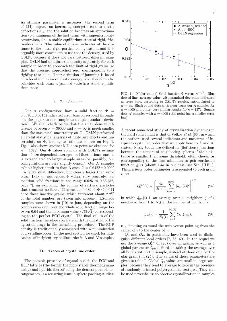
Our A configurations have a solid fraction Φ =0.6370±0.0015 (indicated error bars correspond through-out the paper to one sample-to-sample standard devia-tion). We shall check below that the small density dif-ference between κ = 39000 and κ → ∞ is much smallerthan the statistical uncertainty on Φ. OSLN performeda careful statistical analysis of finite size effects and un-certainty on Φ, leading to estimates shown on Fig. 1.Fig. 1 also shows another MD data point we obtained forn = 1372. Our Φ values coincide with OSLN’s estima-tion of size-dependent averages and fluctuations, once itis extrapolated to larger sample sizes (or, possibly, ourconfigurations are very slightly denser). Our A’ samplesexhibit higher densities than A ones, Φ = 0.6422±0.0002– a fairly small difference, but clearly larger than errorbars. DTS do not report Φ values very precisely, butmention solid fractions in the range 0.625 to 0.63 [52,page 7], on excluding the volume of rattlers, particlesthat transmit no force. This entails 0.639 ≤ Φ ≤ 0.644once those inactive grains, which represent about 2.2%of the total number, are taken into account. LS-madesamples were shown in [10] to jam, depending on thecompression rate, over the whole solid fraction range be-tween 0.64 and the maximum value π/(3

√2) correspond-

ing to the perfect FCC crystal. The final values of thesolid fraction therefore correlate with the duration of theagitation stage in the assembling procedure. The RCPdensity is traditionnally associated with a minimizationof crystalline order. In the next section we check for indi-cations of incipient crystalline order in A and A’ samples.

D. Traces of crystalline order

The possible presence of crystal nuclei, the FCC andHCP lattices (the former the more stable thermodynam-ically) and hybrids thereof being the densest possible ar-rangements, is a recurring issue in sphere packing studies.

0 0.01 0.02 0.03 0.04 0.05

n-1/2

0.63

0.635

0.64

0.645

Φ

A, n=4000, n=1372A’, n=4000OSLN regression

FIG. 1: (Color online) Solid fraction Φ versus n−1/2. Bluedotted line: average value, with standard deviation indicatedas error bars, according to OSLN’s results, extrapolated ton → ∞. Black round dots with error bars: our A samples forn = 4000 and other, very similar results for n = 1372. Squaredot: A’ samples with n = 4000 (this point has a smaller errorbar).

A recent numerical study of crystallization dynamics inthe hard sphere fluid is that of Volkov et al. [66], in whichthe authors used several indicators and measures of in-cipient crystalline order that we apply here to A and A’states. First, bonds are defined as (fictitious) junctionsbetween the centers of neighboring spheres if their dis-tance is smaller than some threshold, often chosen ascorresponding to the first minimum in pair corelationfunction g(r) (about 1.4a in our case, see Sec. III F 1).Then, a local order parameter is associated to each graini, as:

Qlocl (i) =

[

4π

2l + 1

m=l∑

m=−l

|qlm(i)|2]1/2

, (25)

in which qlm(i) is an average over all neighbors j of inumbered from 1 to Nb(i), the number of bonds of i:

qlm(i) =1

Nb(i)

Nb(i)∑

j=1

Ylm(nij), (26)

nij denoting as usual the unit vector pointing from thecenter of i to the center of j.

Q4 and Q6, in particular, have been used to distin-guish different local orders [7, 66, 69]. In the sequel weuse the average Qloc

6 of (26) over all grains, as well as aglobal parameter Q6, defined on taking the average overall bonds within the sample, instead of those of a partic-ular grain i in (25). The values of those parameters aregiven in table I. Global Q6 values are small in large sam-ples, because they tend to average to zero in the presenceof randomly oriented polycrystalline textures. They canbe used nevertheless to observe crystallization in samples

10

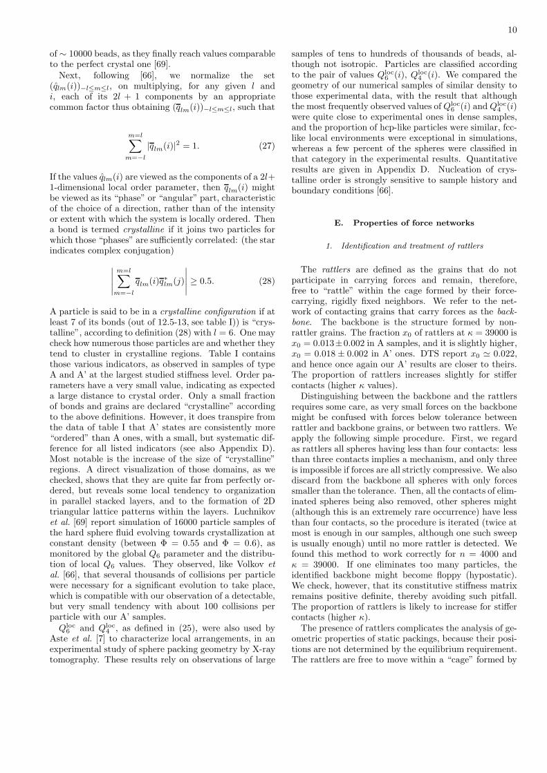
of ∼ 10000 beads, as they finally reach values comparableto the perfect crystal one [69].

Next, following [66], we normalize the set(qlm(i))−l≤m≤l, on multiplying, for any given l andi, each of its 2l + 1 components by an appropriatecommon factor thus obtaining (qlm(i))−l≤m≤l, such that

m=l∑

m=−l

|qlm(i)|2 = 1. (27)

If the values qlm(i) are viewed as the components of a 2l+1-dimensional local order parameter, then qlm(i) mightbe viewed as its “phase” or “angular” part, characteristicof the choice of a direction, rather than of the intensityor extent with which the system is locally ordered. Thena bond is termed crystalline if it joins two particles forwhich those “phases” are sufficiently correlated: (the starindicates complex conjugation)

∣

∣

∣

∣

∣

m=l∑

m=−l

qlm(i)q∗lm(j)

∣

∣

∣

∣

∣

≥ 0.5. (28)

A particle is said to be in a crystalline configuration if atleast 7 of its bonds (out of 12.5-13, see table I)) is “crys-talline”, according to definition (28) with l = 6. One maycheck how numerous those particles are and whether theytend to cluster in crystalline regions. Table I containsthose various indicators, as observed in samples of typeA and A’ at the largest studied stiffness level. Order pa-rameters have a very small value, indicating as expecteda large distance to crystal order. Only a small fractionof bonds and grains are declared “crystalline” accordingto the above definitions. However, it does transpire fromthe data of table I that A’ states are consistently more“ordered” than A ones, with a small, but systematic dif-ference for all listed indicators (see also Appendix D).Most notable is the increase of the size of “crystalline”regions. A direct visualization of those domains, as wechecked, shows that they are quite far from perfectly or-dered, but reveals some local tendency to organizationin parallel stacked layers, and to the formation of 2Dtriangular lattice patterns within the layers. Luchnikovet al. [69] report simulation of 16000 particle samples ofthe hard sphere fluid evolving towards crystallization atconstant density (between Φ = 0.55 and Φ = 0.6), asmonitored by the global Q6 parameter and the distribu-tion of local Q6 values. They observed, like Volkov et

al. [66], that several thousands of collisions per particlewere necessary for a significant evolution to take place,which is compatible with our observation of a detectable,but very small tendency with about 100 collisions perparticle with our A’ samples.

Qloc6 and Qloc

4 , as defined in (25), were also used byAste et al. [7] to characterize local arrangements, in anexperimental study of sphere packing geometry by X-raytomography. These results rely on observations of large

samples of tens to hundreds of thousands of beads, al-though not isotropic. Particles are classified accordingto the pair of values Qloc

6 (i), Qloc4 (i). We compared the

geometry of our numerical samples of similar density tothose experimental data, with the result that althoughthe most frequently observed values of Qloc

6 (i) and Qloc4 (i)

were quite close to experimental ones in dense samples,and the proportion of hcp-like particles were similar, fcc-like local environments were exceptional in simulations,whereas a few percent of the spheres were classified inthat category in the experimental results. Quantitativeresults are given in Appendix D. Nucleation of crys-talline order is strongly sensitive to sample history andboundary conditions [66].

E. Properties of force networks

1. Identification and treatment of rattlers

The rattlers are defined as the grains that do notparticipate in carrying forces and remain, therefore,free to “rattle” within the cage formed by their force-carrying, rigidly fixed neighbors. We refer to the net-work of contacting grains that carry forces as the back-

bone. The backbone is the structure formed by non-rattler grains. The fraction x0 of rattlers at κ = 39000 isx0 = 0.013±0.002 in A samples, and it is slightly higher,x0 = 0.018 ± 0.002 in A’ ones. DTS report x0 ≃ 0.022,and hence once again our A’ results are closer to theirs.The proportion of rattlers increases slightly for stiffercontacts (higher κ values).

Distinguishing between the backbone and the rattlersrequires some care, as very small forces on the backbonemight be confused with forces below tolerance betweenrattler and backbone grains, or between two rattlers. Weapply the following simple procedure. First, we regardas rattlers all spheres having less than four contacts: lessthan three contacts implies a mechanism, and only threeis impossible if forces are all strictly compressive. We alsodiscard from the backbone all spheres with only forcessmaller than the tolerance. Then, all the contacts of elim-inated spheres being also removed, other spheres might(although this is an extremely rare occurrence) have lessthan four contacts, so the procedure is iterated (twice atmost is enough in our samples, although one such sweepis usually enough) until no more rattler is detected. Wefound this method to work correctly for n = 4000 andκ = 39000. If one eliminates too many particles, theidentified backbone might become floppy (hypostatic).We check, however, that its constitutive stiffness matrixremains positive definite, thereby avoiding such pitfall.The proportion of rattlers is likely to increase for stiffercontacts (higher κ).

The presence of rattlers complicates the analysis of ge-ometric properties of static packings, because their posi-tions are not determined by the equilibrium requirement.The rattlers are free to move within a “cage” formed by

11

State dc/a Z Zcr Q6 Qloc6 Qloc,cr

6 xcr 〈ncr〉

A 1.35 12.36 ± 0.03 2.91 ± 0.06 (1.7 ± 0.3) × 10−2 0.392 ± 0.001 0.417 ± 0.003 0.080 ± 0.005 19.8

A’ 1.35 12.50 ± 0.02 3.13 ± 0.11 (1.9 ± 0.5) × 10−2 0.398 ± 0.0005 0.420 ± 0.002 0.104 ± 0.006 54.8

A 1.40 13.11 ± 0.02 2.94 ± 0.06 (1.6 ± 0.3) × 10−2 0.370 ± 0.001 0.394 ± 0.002 0.083 ± 0.006 22.8

A’ 1.40 13.20 ± 0.02 3.16 ± 0.11 (1.8 ± 0.3) × 10−2 0.377 ± 0.0006 0.397 ± 0.003 0.103 ± 0.006 64.5

TABLE I: Indicators of possible incipient crystalline order in states A and A’ at κ = 39000. Z is the coordination number offirst heighbors, Zcr the “crystalline bond” coordination number, Q6 and Qloc

6 the global and (average) local order parameters,

Qloc,cr6 its average value within crystalline regions, xcr the fraction of “crystalline” particles and 〈ncr〉 the mass average of the

number of particles in a “crystalline cluster”. First neighbors are defined here as those closer than distance dc = 1.35a ordc = 1.40a, near the first minimum in g(r).

their backbone neighbors, and there is no obvious way inprinciple to prefer one or another of their infinitely manypossible positions. This renders the evaluation of geo-metric data like pair correlations somewhat ambiguous.Moreover, rattlers, although scarce in frictionless pack-ings, can be considerably more numerous in frictionalones (see Section IV). We therefore specify whether theresults correspond to direct measurements on the con-figurations resulting from the simulations, with rattlersfloating in some positions resulting from compaction dy-namics, or whether rattlers have been fixed, each onehaving three contacts with the backbone (or some previ-ously fixed other rattler). To compute such fixed rattlerpositions with MD, we regard each backbone grain asa fixed object, exert small isotropically distributed ran-dom forces on all rattlers and let them move to a finalequilibrium position (assuming frictionless contacts). Athird possibility is to eliminate rattlers altogether beforerecording geometric data. These are three choices re-ferred to as I, II and III in the sequel, and we denoteobserved quantities with superscripts I, II or III accord-ingly.

Packings under gravity, if locally in an isotropic stateof stress, are expected to be in the same internal state andto exhibit the same properties as the ones that are simu-lated here. In such a situation, individual grain weightsare locally, within an approximately homogeneous sub-system, dominated by the externally imposed isotropicpressure. There is no rattler under gravity, but somegrains are simply feeling their own weight, or perhapsthat of one or a few other grains relying on them. Suchgrains are those that would be rattlers in the absence ofgravity. Instead of freely floating within the cage of theirbackbone neighbors, they are supported by the cage floor.The situation should therefore be similar to that of oursamples after all rattlers have been put in contact withthe force-carrying structure (treatment II), except thatthe small external forces applied to them are all directeddownwards.

2. Coordination numbers

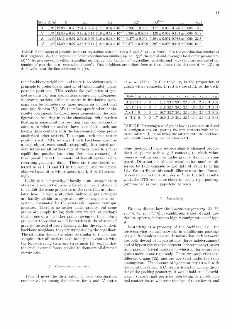
Table II gives the distribution of local coordinationnumber values among the spheres for A and A’ states

at κ = 39000. In this table, xi is the proportion ofgrains with i contacts. If rattlers are stuck to the back-

State x0 x1 x2 x3 x4 x5 x6 x7 x8 x9 x10 x11

A (I) 1.3 0 0 0 11.1 23.2 28.4 22.6 10.3 2.8 0.3 0.02

A’ (I) 1.8 0 0 0 11.6 22.5 28.2 22.3 10.6 2.8 0.3 0.01

A (II) 0 0 0 1.1 10.7 22.7 28.2 22.9 10.9 3.1 0.3 0.02

A’ (II) 0 0 0 1.7 10.9 21.9 28.2 22.5 11.4 3.1 0.3 0.01

TABLE II: Percentages xi of grains having i contacts in A andA’ configurations, on ignoring the rare contacts with or be-tween rattlers (I), or on fixing the rattlers onto the backbonewith small (randomly oriented) forces (II).

bone (method II), one records slightly changed propor-tions of spheres with n ≥ 3 contacts, to which valuesobserved within samples under gravity should be com-pared. Distributions of local coordination numbers ob-served by DTS coincide to the data of Table II within1%. We attribute this small difference to the influenceof contact deflections of order κ−1a in the MD results,while the DTS results are closer to ideally rigid packings(approached as open gaps tend to zero).

3. Isostaticity

We now discuss how the isostaticity property [32, 72,73, 74, 75, 76, 77, 78] of equilibrium states of rigid, fric-tionless spheres, influences high κ configurations of typeA.

Isostaticity is a property of the backbone, i.e. theforce-carrying contact network, in equilibrium packingsof rigid, frictionless spheres. It means that such networksare both devoid of hyperstaticity (force indeterminacy)and of hypostaticity (displacement indeterminacy), apartfrom possible trivial motions in which all force-carryinggrains move as one rigid body. These two properties havedifferent origins [32], and are not valid under the sameassumptions. The absence of hyperstaticity (h = 0 withthe notations of Sec. II C) results from the generic disor-der of the packing geometry. It would hold true for arbi-trarily shaped rigid particles interacting by purely nor-mal contact forces whatever the sign of those forces, and

12

it applies to the whole packing, whatever the contactsthe rattlers might accidentally have with the backbone.The absence of hypostaticity property (except for trivialmechanisms, k = k0), on the other hand, is only guar-anteed for spherical particles with compressive forces inthe contacts, and it applies to the sole backbone.

Due to the isostaticity property, the coordination num-ber should be equal to 6 in the rigid limit on the back-

bone. If Nc is the number of force-carrying contacts,then the global (mechanical) coordination number is

z =2Nc

n(possible contacts of the rattlers are discarded),

and the backbone coordination number is defined as

z∗ =2Nc

n(1 − x0)=

z

1 − x0. z∗, rather than z, has the

limit 6 as κ → +∞. In A samples (κ = 39000) onehas z∗ = 6.074± 0.002 (and hence z ≃ 5.995), the excessover the limit z∗ = 6 resulting from contacts that shouldopen on further decreasing the pressure.

The isostaticity property can be used to evaluate thedensity increase due to finite particle stiffness. To firstorder in the small displacements between P = 0 (orκ = +∞ ) and the current finite pressure state A, onemight use the theorem of virtual work [32], with the dis-placements that bring all overlaps hij to zero, and thecurrent contact forces. Such motions leading to a simul-taneous opening (hij = 0) of all contacts are only possi-ble on networks with no hyperstaticity, because there isno compatibility condition on relative normal displace-ments [32]. This yields an estimate of the increase of thesolid fraction ∆Φ over its value Φ0 in the rigid limit, as

1

Ω

∑

ij

Nijhij = P∆Φ

Φ. (29)

This equality can be rearranged using the Hertz contactlaw (1) to relate Nij to hij , and relation (22). We denoteas Z(α) the moment of order α of the distribution ofnormal forces Nij , normalized by the average over allcontacts:

Z(α) =〈Nα〉〈N〉α . (30)

(29) can be rewritten as:

∆Φ = 35/3Φ1/3Z(5/3)(π

z

)2/3

κ−1. (31)

In the isostatic limit which is approached at large κ, theforce distribution and its moments are determined bythe network geometry, and we observed Z(5/3) = 1.284.Taking for z and Φ the values at the highest studiedstiffness level κ (κ = 39000), this enables us to evalu-ate the density change between those configurations andthe rigid limit as ∆Φ ≃ 1.15 × 10−4. As announced be-fore this is smaller than the statistical uncertainty onΦ, and hence this does not improve our estimation ofthe solid fraction Φ0 of the packing of rigid particles(κ = +∞). Recalling κ−1 = (P/E)2/3, (31) means that

the macroscopic relation between pressure and densityhas the same power law form (P ∝ (∆Φ)3/2) as the con-tact law (N ∝ h3/2). This was observed by OSLN. Itwould hold, because of the isostaticity property in therigid limit, for whatever exponent m in the contact law,the prefactor of the macroscopic relation P ∝ (∆Φ)m

involving Z(1+1/m), a moment of the geometrically de-termined force distribution.

As a consequence of (31), one can simply relate thebulk modulus of frictionless packings to the pressure, asobserved by OSLN too, a property which will be used anddiscussed in paper III [38], which deals with elasticity ofpackings.

4. Force distribution

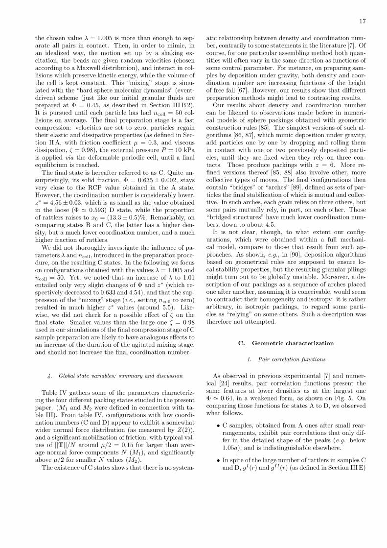
The force distribution we observe in A samples at highκ values approaches the one of a rigid packing, whichdue to isostaticity is a purely geometric property. It isrepresented on Figure 2. The data presented here are av-

0 1 2 3 4 5f

0.001

0.01

0.1

1P(

f)P(f) (A)P(f) (A’)DTS fit

FIG. 2: (Color online) Probability distribution function P (f)of normalized contact forces f = N/〈N〉 in A and A’ configu-rations at high κ. The dashed line is the fit proposed by DTS:P (f) = (3.43f2 + 1.45 − 1.18/(1 + 4.71f)) exp(−2.25f).

eraged over 5 samples. Because of relation (22), all sam-ples prepared at the same pressure have the same aver-age force, and this restores the “self-averaging” property,which OSLN observed to be lacking on using solid frac-tion instead of pressure as the control parameter. Thechoice of Φ as a state variable, because of the finite sizeof the sample causing fluctuations of the threshold Φ0

where P vanishes, is less convenient in that respect.

Fig. 2 also shows that the form proposed by DTS tofit their data is in very good agreement with our results,except perhaps for large forces, for which it is a better fitfor A’ data – thus providing additional evidence that A’samples are closer than A ones to the DTS results.

13

F. Geometric characterization

1. Pair correlation function

Pair correlations should preferably be measured eitherwith method I or method II, as there is no reason to elimi-nate rattlers before studying geometric properties. Com-parisons between pair correlation functions gI(r) andgII(r) (Fig. 3) show very little difference on the scale ofone particle diameter. Results of Fig. 3 are very similarto other published ones (e.g., in DTS), with an apparentdivergence as r → a and a split second peak, with sharpmaxima at r = a

√3 and r = 2a. The pair correlation

1 1.5 2r/a

0

1

2

3

g(r)

gI(r)=g

II(r), A (κ=39000)

FIG. 3: Pair correlation functions gI(r) and gII(r) versusr/a in A samples at κ = 39000. Both definitions coincide onthis scale (only the peak for r → a+ is slightly different).

function should contain a Dirac mass at r = a in thelimit of rigid grains, which broadens into a sharp peakfor finite contact stiffness. The weight of this Dirac termor peak in the neighbor intercenter distance probabilitydistribution function 4π n

Ωr2g(r) = 24(r2/a3)Φg(r) is co-ordination number z, and the shape of the left shoulderof the peak at finite κ is directly related to the forcedistribution P (N):

(For δ > 0) g(a − δ) =za3E

√aδ

48Φ(a − δ)2P (

E√

aδ3/2

3).

This explains the observation by OSLN [31] of the widthof the g(r) peak decreasing approximatively as ∆Φ, whileits height increases as (∆Φ)−1, as the threshold densityΦ0 is approached from above. The form of the distribu-tion of contact forces, which is determined by the geom-etry of the isostatic backbone, remains exactly the samefor all small enough values of ∆Φ, with a scale factorproportional to ∆Φ3/2, due to Eqns. 22 and 31.

The sharp drop of g(r) at r = a√

3 and r = 2a wasfound by DTS to go to a discontinuity in the rigid particlelimit. This can be understood as follows. Each spherehas a number of first contact neighbors (z on average)

at distance r = a if the grains are rigid, and a numberof second contact neighbors (i.e. particles not in contactwith it, but having a contact with at least one of itsfirst contact neighbors). Such second contact neighborswill make up for a significant fraction of particles withtheir centers at a distance r ≤ 2a, but none of them canbe farther away. Futhermore, this leads to a systematicdepletion of the corona 2a < r < 2a + δ (with 0 < δ < a)by steric exclusion.

2. Near neighbor correlations

As r → a+, pair correlations are conveniently ex-pressed with the gap-dependent coordination numberz(h). z(h) is the average number of neighbors of onesphere separated by an interstice narrower than h. z(0) isthe usual contact coordination number z. Function z(h)has three possible different definitions zI , zII and zIII

according to the treatment of rattlers. All three of themwere observed to grow as z(0)+ Ch0.6 for h smaller thanabout 0.3a, constant C taking slightly different values forzI , zII and zIII . zIII(h) is equal to z∗ for h = 0, and isvery well fitted with the value C = 11 found by DTS [52,Fig. 8]. z(h) deviates from this power law dependencecorresponding to the rigid limit for small h, of the or-der of the typical overlap κ−1, as shown on Fig. 4. Thispower law corresponds to g(r) diverging as (r − a)−0.4

as r → a+. Silbert et al., in a recent numerical study

10-3

10-2

10-1

h

10-1

100

101

z(h)

-6

zII(h), κ=39000

zII(h), κ=18000

zII(h), κ=8400

slope 0.6

FIG. 4: (Color online) Coordination number of near neighborsfunction of interstice h. The power law regime extends tosmaller and smaller h values as κ increases.

of states with high levels of rigidity [79] (κ > 106), re-port observing zI(h) to grow with an exponent closer to0.5, although somewhat dependent on the choice of theh interval for the fit. However this does not contradictour main conclusion that different numerical approachestrack the same RCP state in the rigid limit.

14

3. Other properties of contact networks

Ignoring rattlers (method III) one may record the den-sity of specific particle arrangements in the backbone.We thus find the contact network (joining all centers ofinteracting particles by an edge) to comprise a numberof equilateral triangles, such that on average each back-bone grain belongs to 2.04 ± 0.04 triangles. In the rigidlimit this gives a Dirac term for θ = π/3 in the distri-bution of angles θ between pairs of contacts of the samegrain. Tetrahedra are however very scarce (as observedby DTS), involving about 2.5% of the beads, and pairsof tetrahedra with a common triangle are exceptional (5such pairs in 5 samples of 4000 beads). Pairs of trianglessharing a common base are present with a finite density,which explains the discontinuous drop at r = a

√3 of

g(r), this being the largest possible distance for such apopulation of neighbor pairs.

G. Conclusions

We summarize here the essential results of Section III,about frictionless packings.

1. Uniqueness of the RCP state

Our numerical evidence makes a strong case in favorof the uniqueness of the simulated rigid packing statemade with frictionless spheres under isotropic pressure.Specifically, we observed quantitative agreements withother published results [31, 52] in the coordination num-bers, the force distributions, the pair correlations andthe frequency of occurrence of local contact patterns,even though different numerical methods have been used.The small remaining differences in solid fraction, propor-tion of rattlers, and probability of large contact forces allcorrelate with the duration of agitated assembling stage,which can be measured in terms of numbers of collisionsper grain at a given density. This duration directly cor-relates to the packing fraction and to the small amountof crystalline order in the samples. We therefore checkedin an accurate, quantitative way the traditional viewsabout random close packing (RCP). The RCP state canbe defined in practice as the unique state in which rigidfrictionless spherical beads assemble in a static equilib-rium state under isotropic pressure, in the limit of fastcompression, so that the slow evolution towards crystal-lization has a negligible influence. The Lubachevsky-Stillinger algorithm tends to produce packings with asmall but notable crystalline fraction.

2. Relevance of MD simulations, role of micromechanical

parameters

The uniqueness of the RCP implies that dynamical pa-rameters ζ and I have no influence on the frictionlesspacking structures, at least in the limit of fast compres-sion rates.

Standard MD methods compare well with specificallydesigned methods that deal with rigid particles, andprove able to approach the rigid limit with satisfactory, ifadmittedly smaller, accuracy. Recalling that κ = 39000corresponds to glass beads under 10 kPa, it seems thatlaboratory samples under usual conditions might in prin-ciple (if friction mobilization can be suppressed) ap-proach the ideal (rigid particle) RCP state.

Moreover, the time scales to assemble samples in MDsimulations, if compared to estimated preparation timesin the laboratory with such techniques as controlled plu-viation, has the right order of magnitude. This meansthat the assembling proces is rather fast in experimentalpractice when grains are deposited under gravity, whichexplains why densities above RCP are not directly ob-tained. Of course, in practice, many procedures produceanisotropic states. Anisotropic packings of rigid, fric-tionless balls, under other confining stresses than a hy-drostatic pressure, should differ from the RCP state, andthe numerical simulations of gravity deposited packingsof frictionless beads of refs. [24, 25] could be analysed inthis respect. We chose here to study ideal preparationmethods, and we only deal with isotropic systems.

3. Approach to isostaticity in the rigid limit

We checked that bead packings under typical labora-tory pressures such as 10 kPa might closely approach theisostaticity property of rigid frictionless packings. Weshowed that some observations made by O’Hern et al. [31]on pressure or bulk modulus dependence on density, andon the shape of the first peak of g(r) were direct conse-quences of this remarkable property.

IV. LOW-PRESSURE STATES OF FRICTIONALPACKINGS OBTAINED BY DIFFERENT

PROCEDURES

A. Introduction

It is well known that the introduction of friction ingranular packings tends in general to reduce density andcoordination number, as observed in many recent numer-ical simulations (see e.g. [24, 25, 26, 27]), and that fric-tional granular assemblies, unlike frictionless ones, canbe prepared in quite a large variety of different states.In the field of soil mechanics, sand samples are tradition-nally classified by their density [11, 12, 13], which deter-mines behaviors that have been observed in simulations

15

of model systems as well [21, 27]. (Inherent anisotropy

of the fabric, i.,e., the one due to the assembling pro-cess, rather than induced by anisotropic stresses, is asecondary, less influential state variable [14, 15]). Engi-neering studies on sands usually resort to a conventionaldefinition of minimum and maximum densities, based onstandardized procedures [80].

The motivation of the present study is to explore therange of accessible packing states, as obtained by dif-ferent numerical procedures that produce homogeneousand isotropic periodic samples. We therefore chose to by-pass the painstaking computations needed to mimic ac-tual laboratory assembling methods, but we argue thatour procedures produce plausible structures with similarproperties.

One key result is that density alone does not determinethe internal state of an isotropic packing, because thecoordination number can vary independently.

The A-type configurations obtained without friction inSection IVB are local density maxima in configurationspace (see Sec. III C 1). Hence compaction methods canbe regarded as strategies to circumvent the mobilizationof intergranular friction forces. Two such procedures arestudied here, in a simplified, idealized form: lubricationand vibration. We also simulate, as a reference, a statewhich can be regarded as a loose packing limit, at leastwith a definition relative to one assembling method andfriction coefficient µ = 0.3 ; and we prepare, as an in-teresting limit from a theoretical point of view, infinitefriction samples.

Assembling procedures are described in Section IVB,geometric aspects are studied in Section IV C, and con-tact network properties in Section IVD. Section IVEsummarizes the results.

B. Assembling processes for frictional grains

Just like in the frictionless case, for each one of thepacking states, we prepare 5 samples of 4000 beads, overwhich results are averaged, error bars corresponding tosample-to-sample fluctuations. The equilibrium criteriaare those of Section III B 2, supplemented with a similarcondition on moments. To identify rattlers, we use theprocedure defined in Section III E 1, which is adapted tothe case of frictional grains: spheres with as few as twocontacts may carry forces (even large ones, as we shallsee) and should not be regarded as rattlers.

1. Looser packings compressed with final friction coefficient

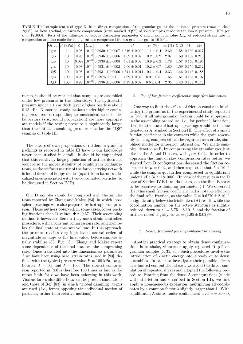
We used direct compression of a granular gas in thepresence of friction (µ = 0.3), another standard numer-ical procedure [26, 27, 28], in which the obtained den-sity and coordination number are decreasing functionsof µ [24, 25, 26, 27]. This produces rather loose sam-ples hereafter referred to as D (B and C ones, to be

defined further, denoting denser ones, closer to A, butarguably more “realistic”). D samples were made withexactly the same method as A ones (see Sec. III B 2),except that the friction coefficient µ = 0.3 was used in-stead of µ = 0. In principle, D configurations shoulddepend on initial compaction dynamics: increasing therate of compression could produce denser equilibratedpackings, just like a larger height of free fall, whencea larger initial kinetic energy, increases the density ofconfigurations obtained by rain deposition under grav-ity [67]. We request the reduced compression rate I, de-fined in (23), not to exceed a prescribed maximum valueImax. The choice of Imax = 10−3 and ζ = 0.98 yieldssolid fractions Φ = 0.5923±0.0006 and backbone coordi-nation numbers z∗ = 4.546±0.009, with a rattler fractionx0 = (11.1±0.4)%. These data correspond to P = 1 kPa(or κ ≃ 181000). Very similar results are obtained onusing a different, but low enough pressure, such as 10or even 100 kPa, as remarked in [41] (where 2D sam-ples were assembled by oedometric compression), and asindicated in table III. However, a quasistatic compres-sion from P = 1 kPa to 10 or 100 kPa produces slightlydifferent states at the same pressure. The influence of ζshould disappear in the limit of slow compression, I → 0.A practical definition of a (µ-dependent) limit of loosepacking obtained by direct compression, can thereforebe proposed as the I → 0 limit of our D states. Asreported in table III, a value of the damping parameterten times as small as the standard one ζ = 0.98 results inquite similar configuration properties, on compressing aloose granular gas under P = 10 kPa, with Imax = 10−3.So did in fact faster compressions, with Imax = 10−1 ,keeping ζ = 0.98. The data of Table III thus suggestthat we very nearly achieved the independence on dy-namical parameters that is expected in the I → 0 limitwith our choice of control parameters. We note, however,that other possible definitions of a random loose packing,such as the one by Onoda and Liniger [81] result in dif-ferent (smaller) solid fractions. Looser arrangements ofequal-sized spherical particles can also be stabilized withadhesive contact forces, e.g. on introducing the capillaryattractions produced by the menisci formed by a wettingfluid in the interstices between neighboring grains [82].

In addition to packing fraction Φ, coordination num-ber z∗, fraction of rattlers x0, Table III lists the reducedsecond moment Z(2) of the normal force distribution, asdefined in (30), the proportion of two-coordinated beads(to be discussed in Section IVD), x2, and the average val-ues of ratios ||T||/N (friction mobilization) among con-tacts carrying normal forces larger and smaller than theaverage, respectively denoted as M1 and M2. As a resultof some amount of quasistatic compression of the initialassembly, the width of the force distribution decreases,as witnessed by smaller values of Z(2) in table III, andso does the mobilization of friction, as measured by M1

and M2. The effects of compression on the structure andthe forces are further studied in paper II [37]. On com-paring numerically simulated loose packings to experi-

16

TABLE III: Isotropic states of type D, from direct compression of the granular gas at the indicated pressure (rows marked“gas”), or from gradual, quasistatic compression (rows marked “QS”) of solid samples made at the lowest pressure 1 kPa (orκ ≃ 181000). Tests of the influence of viscous dissipation parameter ζ and maximum value Imax of reduced strain rate incompression are also made for configurations compressed from a granular gas to 10 kPa.

Origin P (kPa) ζ Imax Φ z∗ x0 (%) x2 (%) Z(2) M1 M2

gas 1 0.98 10−3 0.5930 ± 0.0007 4.546 ± 0.009 11.1 ± 0.4 2.39 1.58 0.160 0.217

gas 10 0.98 10−3 0.5946 ± 0.0006 4.59 ± 0.02 10.2 ± 0.2 2.07 1.59 0.159 0.213

gas 10 0.098 10−3 0.5938 ± 0.0008 4.61 ± 0.02 10.9 ± 0.2 1.79 1.57 0.150 0.194

gas 10 0.98 10−1 0.5931 ± 0.0002 4.60 ± 0.01 10.2 ± 0.7 1.80 1.59 0.159 0.212

QS 10 0.98 10−3 0.5931 ± 0.0006 4.641 ± 0.011 10.1 ± 0.4 2.33 1.46 0.146 0.188

gas 100 0.98 10−3 0.5975 ± 0.001 4.69 ± 0.02 8.9 ± 0.5 1.66 1.61 0.153 0.197

QS 100 0.98 10−3 0.5936 ± 0.0006 4.79 ± 0.02 8.6 ± 0.4 2.05 1.40 0.138 0.178

ments, it should be recalled that samples are assembledunder low pressures in the laboratory: the hydrostaticpressure under a 1 cm thick layer of glass beads is about0.15 kPa. Numerical configurations under higher confin-ing pressures corresponding to mechanical tests in thelaboratory (e.g., sound propagation) are more appropri-ate models if the testing pressure is significantly largerthan the initial, assembling pressure – as for the “QS”samples of table III.

The effects of such proportions of rattlers in granularpackings as reported in table III have to our knowledgenever been studied in detail. It should be emphasizedthat this relatively large population of rattlers does notjeopardize the global stability of equilibrium configura-tions, as the stiffness matrix of the force-carrying networkis found devoid of floppy modes (apart from harmless, lo-calized ones associated with two-coordinated particles, tobe discussed in Section IVD).

Our D samples should be compared with the simula-tions reported by Zhang and Makse [83], in which loosesphere packings were also prepared by isotropic compres-sion. Those authors observed, in some cases, lower pack-ing fractions than D values, Φ ≃ 0.57. Their assemblingmethod is however different: they use a strain-controlledprocedure, with a constant compression rate, and then re-lax the final state at constant volume. In this approach,the pressure reaches very high levels, several orders ofmagnitude as large as the final value, before samples fi-nally stabilize [83, Fig. 3]. Zhang and Makse reportsome dependence of the final state on the compressingrate. Once translated into the dimensionless parameterI we have been using here, strain rates used in [83], de-fined with the typical pressure value P = 100 kPa, rangebetween I = 0.1 and I = 100. The slowest compres-sion reported in [83] is therefore 100 times as fast as theupper limit for ǫ we have been enforcing in this work.Viscous forces also differ between the present simulationsand those of Ref. [83], in which “global damping” termsare used (i.e., forces opposing the individual motion ofparticles, rather than relative motions).

2. Use of low friction coefficients: imperfect lubrication

One way to limit the effects of friction consist in lubri-cating the grains, as in the experimental study reportedin [84]. If all intergranular friction could be suppressedin the assembling procedure, i.e., for perfect lubrication,then the structure of isotropic packings would be the onedenoted as A, studied in Section III. The effect of a smallfriction coefficient in the contacts while the grain assem-bly is being compressed can be regarded as a crude, sim-plified model for imperfect lubrication. We made sam-ples, denoted as B, by compressing the granular gas, justlike in the A and D cases, with µ = 0.02. In order toapproach the limit of slow compression rates better, westarted from D configurations, decreased the friction co-efficient to µ = 0.02, and then requested that I < 10−4

while the samples got further compressed to equilibriumunder 1 kPa (κ ≃ 181000). (In view of the results in the Dcase of Section IVB 1, we do not expect the final B stateto be sensitive to damping parameter ζ.) We observedthat this small friction coefficient had a notable effect onthe final solid fraction, as the value Φ = 0.6270± 2.10−4

is significantly below the frictionless (A) result, while thecoordination number on the active structure is slightlyreduced, down to z∗ = 5.75± 8.10−3, and the fraction ofrattlers raised slightly, to x0 = (1.95 ± 0.02)%.

3. Dense, frictional packings obtained by shaking

Another practical strategy to obtain dense configura-tions is to shake, vibrate or apply repeated “taps” ongranular samples [5, 35, 36]. Such procedures involve theintroduction of kinetic energy into already quite denseassemblies. In order to investigate their possible effectsat a limited computational cost, we avoid the direct sim-ulation of repeated shakes and adopted the following pro-cedure. Starting from the dense A configurations (madewithout friction and described in Section III), we firstapply a homogeneous expansion, multiplying all coordi-nates by a common factor λ slightly larger than 1. Withequilibrated A states under confinement level κ = 39000,

17

the chosen value λ = 1.005 is more than enough to sep-arate all pairs in contact. Then, in order to mimic, inan idealized way, the motion set up by a shaking ex-citation, the beads are given random velocities (chosenaccording to a Maxwell distribution), and interact in col-lisions which preserve kinetic energy, while the volume ofthe cell is kept constant. This “mixing” stage is simu-lated with the “hard sphere molecular dynamics” (event-driven) scheme (just like our initial granular fluids areprepared at Φ = 0.45, as described in Section III B 2).It is pursued until each particle has had ncoll = 50 col-lisions on average. The final preparation stage is a fastcompression: velocities are set to zero, particles regaintheir elastic and dissipative properties (as defined in Sec-tion II A, with friction coefficient µ = 0.3, and viscousdissipation, ζ = 0.98), the external pressure P = 10 kPais applied via the deformable periodic cell, until a finalequilibrium is reached.

The final state is hereafter referred to as C. Quite un-surprisingly, its solid fraction, Φ = 0.635 ± 0.002, staysvery close to the RCP value obtained in the A state.However, the coordination number is considerably lower,z∗ = 4.56± 0.03, which is as small as the value obtainedin the loose (Φ ≃ 0.593) D state, while the proportionof rattlers raises to x0 = (13.3 ± 0.5)%. Remarkably, oncomparing states B and C, the latter has a higher den-sity, but a much lower coordination number, and a muchhigher fraction of rattlers.

We did not thoroughly investigate the influence of pa-rameters λ and ncoll, introduced in the preparation proce-dure, on the resulting C states. In the following we focuson configurations obtained with the values λ = 1.005 andncoll = 50. Yet, we noted that an increase of λ to 1.01entailed only very slight changes of Φ and z∗ (which re-spectively decreased to 0.633 and 4.54), and that the sup-pression of the “mixing” stage (i.e., setting ncoll to zero)resulted in much higher z∗ values (around 5.5). Like-wise, we did not check for a possible effect of ζ on thefinal state. Smaller values than the large one ζ = 0.98used in our simulations of the final compression stage of Csample preparation are likely to have analogous effects toan increase of the duration of the agitated mixing stage,and should not increase the final coordination number.

4. Global state variables: summary and discussion

Table IV gathers some of the parameters characteriz-ing the four different packing states studied in the presentpaper. (M1 and M2 were defined in connection with ta-ble III). From table IV, configurations with low coordi-nation numbers (C and D) appear to exhibit a somewhatwider normal force distribution (as measured by Z(2)),and a significant mobilization of friction, with typical val-ues of ||T||/N around µ/2 = 0.15 for larger than aver-age normal force components N (M1), and significantlyabove µ/2 for smaller N values (M2).

The existence of C states shows that there is no system-

atic relationship between density and coordination num-ber, contrarily to some statements in the literature [7]. Ofcourse, for one particular assembling method both quan-tities will often vary in the same direction as functions ofsome control parameter. For instance, on preparing sam-ples by deposition under gravity, both density and coor-dination number are increasing functions of the heightof free fall [67]. However, our results show that differentpreparation methods might lead to contrasting results.

Our results about density and coordination numbercan be likened to observations made before in numeri-cal models of sphere packings obtained with geometricconstruction rules [85]. The simplest versions of such al-gorithms [86, 87], which mimic deposition under gravity,add particles one by one by dropping and rolling themin contact with one or two previously deposited parti-cles, until they are fixed when they rely on three con-tacts. Those produce packings with z = 6. More re-fined versions thereof [85, 88] also involve other, morecollective types of moves. The final configurations thencontain “bridges” or “arches” [89], defined as sets of par-ticles the final stabilization of which is mutual and collec-tive. In such arches, each grain relies on three others, butsome pairs mutually rely, in part, on each other. Those“bridged structures” have much lower coordination num-bers, down to about 4.5.

It is not clear, though, to what extent our config-urations, which were obtained within a full mechani-cal model, compare to those that result from such ap-proaches. As shown, e.g., in [90], deposition algorithmsbased on geometrical rules are supposed to ensure lo-cal stability properties, but the resulting granular pilingsmight turn out to be globally unstable. Moreover, a de-scription of our packings as a sequence of arches placedone after another, assuming it is conceivable, would seemto contradict their homogeneity and isotropy: it is ratherarbitrary, in isotropic packings, to regard some parti-cles as “relying” on some others. Such a description wastherefore not attempted.

C. Geometric characterization

1. Pair correlation functions

As observed in previous experimental [7] and numer-ical [24] results, pair correlation functions present thesame features at lower densities as at the largest oneΦ ≃ 0.64, in a weakened form, as shown on Fig. 5. Oncomparing those functions for states A to D, we observedwhat follows.

• C samples, obtained from A ones after small rear-rangements, exhibit pair correlations that only dif-fer in the detailed shape of the peaks (e.g. below1.05a), and is indistinguishable elsewhere.

• In spite of the large number of rattlers in samples Cand D, gI(r) and gII(r) (as defined in Section III E)

18

TABLE IV: Isotropic states (κ ≃ 39000 for A and C, κ ≃ 181000 for B and D) for different assembling procedures.

Procedure Φ z∗ x0 (%) x2 (%) Z(2) M1 M2

A 0.6370 ± 0.0002 6.074 ± 0.0015 1.3 ± 0.2 0 1.53 0 0

B (µ0 = 0.02) 0.6271 ± 0.0002 5.80 ± 0.007 1.95 ± 0.02 ∼ 10−4 1.52 0.016 0.018

C (λ = 1.005) 0.635 ± 0.002 4.56 ± 0.03 13.3 ± 0.5 2.64 1.65 0.135 0.181

D 0.5923 ± 0.0006 4.546 ± 0.009 11.1 ± 0.4 2.39 1.58 0.160 0.217

FIG. 5: Pair correlation functions g(r) (definitions gI(r) andgII(r) coincide on this scale) for configurations B, C, D.

cannot be distinguished on the scale of Fig. 5.

• The depth of the trough between r/a = 1.1 andr/a = 1.5 increases with density.

• The integral below the peaks correlates with den-sity, but the height and sharpness of the drop atr/a =

√3 and r/a = 2 correlate with coordina-

tion number (which is larger for B than for C), inagreement with the interpretation of such featuressuggested in Sec. III F.

2. Near neighbor coordination numbers

The gap-dependent coordination number zII(h) isshown on Fig. 6 for samples A to D. Fig. 6 shows that,

FIG. 6: (Color online) Coordination number for neighbors atdistance ≤ h, zII(h), for configurations A (red, upper dashedline), B (blue, middle dashed line), C (black, solid line) andD (green, bottom dashed line).

as might have been intuitively expected, z(h) correlateswith coordination number for small h and with densityfor larger distances, h ≥ 0.04a. We preferably use defi-nition zII , which is obtained on bringing the rattlers incontact with the backbone with small, random forces, asexplained in Sec. III E. zII(h) can be thought of as morephysically meaningful than zI(h), which directly resultsfrom the simulation of the packing, and is somewhat am-biguously defined because the positions of the rattlers arenot specified. Functions zII(h) corresponding to B andC states cross each other for h ≃ 0.02a.

zI(h) and zII(h) might be fitted by power laws:

zI(h) = BI + AIhβI

zII(h) = BII + AIIhβII

(32)

Figs 7, 8 and 9 display zI(h) − BI and zII(h) − BII

as functions of h on logarithmic plots for samples D, Band C (due to the influence, at short distance, of contactdeflections on z(h) data, fit parameters BI and BII area little smaller than z and zII(0)). For h values smallerthan 10−4, the lowest limit on the axis on Figs. 7, 9 and 8,

19

the gap h is of the same order as elastic deflections, κ−1,and we do not observe simple power laws (as on Fig. 4).

These figures (on which the corresponding values of

FIG. 7: (Color online) zI(h) − z (blue) and zII(h) − zII(0)(black) versus h on doubly logarithmic plot for D samplesat lowest pressure. The slopes of the corresponding dottedstraight lines (power law fits) are βII = 0.51 and βI = 0.35(see Eqn. 32).

FIG. 8: (Color online) Same as Fig. 7, for B samples. Dottedlines have slopes βII = 0.56 and βI = 0.45.

z ≃ zI(0) and zII(0) are also provided) show that zI andzII have quite different h dependences. This should beaccounted for on studying the closing of contacts due tocompression (see paper II [37]). As a result of the com-putation leading to the equilibrated state, many pairs ofneighbors end up separated by a very small interstice,so that zI − z already reaches values larger than 0.3 forh = 10−4a in samples C and D. zI then grows with hmore slowly than zII , with βII > βI , and a power law fitof lesser quality. Exponent βII , which should be regardedas a more intrinsic quantity than βI , appears to correlatewith solid fraction. It has the same value 0.6 in samples

FIG. 9: (Color online) Same as Fig. 7, for C samples. Slopesof dotted straight lines: βII = 0.6 and βI = 0.37.

C and A (Figs 9 and 4), decreases to 0.55 in the inter-mediate density state B, and to 0.51 for the least denseone, D. The power-law form of zII extends to h ≃ 0.3 inconfiguration A, to about h ≃ 0.2 in configuration B, andonly to 0.04 and 0.05 for C and D. Such limited powerlaw ranges preclude comparisons with the experimentaldata of [7].

One has zI(0) ≃ z as a very good approximation, sincecontacts carrying no force in the equilibrated state ob-tained by MD are very scarce. zII(0), on the other hand,is the geometric coordination number once all rattlers arepushed against the backbone. It is larger than the me-

chanical coordination number, z. Specifically, becauseall rattlers, in treatment II, are dealt with as frictionless,one has:

zII(0) = z + 6x0 −2Nrr

n, (33)

in which Nrr is the final number of contacts betweenrattlers once they are positioned against the backbone.Value of zII(0) can be read on Fig. 6. As pointed outin Section III E 1, they can be compared to coordinationnumber values of samples under gravity. The results ofSilbert et al. [24, Figs. 2 and 3], with µ = 0.3, corre-spond approximately with our D samples: Φ ≃ 0.59 andzII(0) ≃ 5. The systems simulated in [24] are howevernot isotropic. None of the samples made under gravityin [24, 25] appears to resemble our C state.

3. Absence of crystalline order, local order parameters

All indicators of incipient crystalline order given in Ta-ble I for frictionless A samples take lower values in statesB and D, while C configurations, due to their geometricproximity, are close to A ones in this respect. Alreadyscant in dense configurations assembled without friction,traces of crystallization are thus negligible in looser ones

20

obtained with frictional beads. Like for A samples, nu-merical data on configurations around one sphere i, ascharacterized by the pair (Q4(i), Q6(i)), used by Aste et

al. [7], are presented for states B, C, and D and com-pared to their experimental results in Appendix D. Itis observed that local disordered environments aroundone grain are very similar in numerical and experimen-tal configurations of equal densities, while local HCP-likearrangements occur with similar (low) frequencies, andFCC-like ones are present in the laboratory, but not de-tected in simulations.

D. Properties of force networks

1. Local contact coordination numbers

The distribution of local coordinations is given in Ta-ble V, for both mechanical (I) and geometric (II) defini-

State x0 x1 x2 x3 x4 x5 x6 x7 x8 x9 x10

B (I) 1.95 0 0.05 0.5 16.3 26.9 27.5 18.4 7.1 1.4 0.1

C (I) 13.3 0 2.6 15.1 26.5 23.4 13.2 4.8 0.9 0.15 0

D (I) 11.1 0 2.4 13.8 29.1 25.6 13.3 4.0 0.7 0.03 0

B (II) 0 0 0 2.1 15.3 26.5 27.5 18.9 7.8 1.6 0.2

C (II) 0 0 0 18.9 22.8 27.0 18.6 9.3 2.8 0.5 0.1

D (II) 0 0 0 17.2 25.4 29.0 18.5 7.7 1.9 0.3 0

TABLE V: Percentage xi of grains having i contacts in con-figurations B, C and D, on ignoring contacts with or betweenrattlers (I), or on fixing them onto the backbone with small,random forces (II).

tions of contacts, for states B to D. Compared to the Acase (Table II), the distribution is shifted to lower values,with 4 and 5 the most frequent ones (rather than 6) in lowcoordinated packings C and D. Those samples also havequite a large population of three-coordinated spheres,and a notable one of divalent (two-coordinated) parti-cles. This contrasts with the frictionless case for whichx2 = x3 = 0. Without friction, divalent spheres, fromEqn. 20, written with Nc = 2, Nf = 3, h = 0, would im-ply a mechanism and therefore an instability, and three-coordinated ones, in the absence of external forces andcohesion, cannot be equilibrated by non-vanishing nor-mal forces the net effect of which necessarily pushes themaway from the plane defined by the three centers of theirtouching neighbors (the non-generic case with the foursphere centers within the same plane leading to an insta-bility). Spheres with three contacts therefore need somemobilization of friction to transmit non-vanishing forcesin an equilibrium configuration, for tangential compo-nents are requested to cancel this net repulsion. TheCoulomb condition then restricts such possible configu-rations to flat enough tetrahedra for contact forces toremain within the friction cone. This explains the smallvalue of x3 in low friction (µ = 0.02) B samples.

2. The special case of divalent grains

With friction, the small structure formed by one spherehaving two contacts with fixed objects (Fig. 10), due toEqn. 19, in which the number of degres of freedom (6)is equal to the number of contact force coordinates, hasa degree of force indeterminacy equal to its number ofindependent mechanisms: h = k. In fact, both numbersare equal to 1. Self-balanced contact forces (see first partof Fig. 10) are oriented along the line joining the two con-tacts, just like in the corresponding 2D case dealt within [47], and their amplitude is a free parameter (the de-gree of “wedging” of the grain in the corner formed byits two neighbors [47]). Such a possibility requires inpractice that the angle, which we denote as α (Fig. 10),between the line joining the centers of 1 and 2 and theone joining the contact points be smaller than the angleof friction, for the total contact force to stay within theCoulomb cone. In C and D samples, we observed tanα tobe distributed rather evenly between 0 and µ, while theintensity of forces transmitted by divalent spheres rangedfrom 0 to a few times Pa2. The mechanism associated

1

1

1

N

N

T

T21

21

3131

1

(a)

(b)

α

α

2

23

3

FIG. 10: Equilibrium and free motion (mechanism) of onesphere (marked 1) with two contacts (with particles marked2 and 3). (a): in the plane of the three centers, normal andtangential components of the two contact forces balance alongthe line joining the contact points (dotted line). (b): seenfrom above, along the direction of the line of the centers ofspheres 2 and 3, sphere 1 can move and occupy the differentpositions depicted with dashed lines, its center describing thedotted circle around the 2-3 axis.

with divalent spheres is a free rolling motion on the twocontacts, the line joining the contact points being theinstantaneous axis of rotation, as shown on fig. 10(b).In this motion, it is readily checked (see Appendix E)that the rules given in Appendix B for the evolution ofcontact forces in the case of rolling and pivoting specifythat contact forces will remain carried by the line join-ing the two contacts, with a constant intensity, as suchcontacts move on the surface of the fixed spheres. Such

21

forces will do no work and the kinetic energy of the mo-bile sphere as well as the elastic energy stored in its twocontacts will be kept constant. The equilibrium of thedivalent particle is thus marginally stable, with matrix

K(2) causing zero acceleration to the free motion. How-

ever, such a motion does affect the balance of moments

on spheres marked 2 and 3 on Fig. 10, since the con-stant force is applied at a point that is moving on theirsurface. Therefore the stability of such free motions, asregards the global contact network, requires some addi-tional analysis – which is tackled in Appendix E, whereit is concluded that the packing remains stable. Unlikein frictionless packings [32, 91], mechanisms in the pres-ence of friction do not necessarily lead to instabilities. On

building the constitutive stiffness matrix K(1) in the sam-

ples we studied, we could check that no other mechanismwas present on the backbone than those rolling motionsof divalent spheres. Once some stiffness element is in-troduced to impede the free motion of divalent spheres,one can e.g. check that the Cholesky factorization of thestiffness matrix only involves strictly positive terms onthe diagonal.

There can be no contact between two divalent spheres,as the simultaneous equilibrium of each of them with twoforces carried by the line joining its two contact points,as on Fig. 10, is impossible.

3. Degree of force indeterminacy

On the backbone, with n(1 − x0) spheres and N∗f =

6n(1 − x0) + 3 degrees of freedom, one has on averagez∗n(1 − x0)/2 contacts and k = 3 + x2n independentmechanisms, hence a degree of force indeterminacy (hy-perstaticity), from (19), given by:

h = N∗f

z∗ − z∗04

= N∗f

z∗∗ − 4

4, with

z∗0 = 4 − 2x2

3(1 − x0)and

z∗∗ = z∗ +2x2

3(1 − x0)

(34)

The backbone is devoid of force indeterminacy (h = 0)when its coordination number is equal to z∗0 . Becauseof the mechanisms associated with divalent beads z∗0 isstrictly smaller than 4. Alternatively, one can define a“corrected” backbone coordination number z∗∗, as writ-ten in (34), which is equal to 4 in the absence of forceindeterminacy. As to the global mechanical coordinationnumber z0 corresponding to the absence of force indeter-minacy, its value, given by

z0 = 4(1 − x0) −2x2

3, (35)

is well below 4. From the data of table V, z0 is about 3.45in state C and 3.54 for D (while z is close to 4). Althoughh is relatively small compared to the number of degrees

of freedom Nf , the samples with friction and low coordi-nation are still notably hyperstatic – a conclusion sharedby other studies [24], which we reach here in the slightlydifferent context of packings in a uniform state of stress.Unlike for frictionless sphere assemblies, there is actuallyno special reason to expect packings with intergranularfriction to become isostatic in the rigid contact limit. Theessential difference is that contact forces can no longer beregarded as enforcing hard geometric constraints like im-penetrability, and hyperstatic configurations do not re-quire exceptional arrangements or matching of particlesizes as in the frictionless case [32, 74, 76, 92].

Unlike us, Zhang and Makse [83] speculate that iso-static packings could be obtained in the limit of slowcompressions of samples with ordinary values of µ. Thisis however due to a divergence of interpretation, ratherthan a contradiction in numerical results, since their min-imum coordination numbers z∗, excluding rattlers, aresimilar to ours, z∗ ≃ 4.5. Zhang and Makse could onlyapproach configurations devoid of hyperstaticity on set-ting the friction coefficient to infinity (see Section IVD 6below). The degree of force indeterminacy per degreeof freedom on the backbone is still equal, from (34), to0.141 in D samples and 0.145 in C ones, and varies verylittle with compression rate in the range we explored,which extends to significantly smaller values than theones used in [83], as stressed above. It is not obviouswhether special experimental situations might occur inwhich real granular assemblies approach vanishing de-grees of hyperstaticity.

4. Distribution of normal forces

Since the force-carrying structure maintains a non-vanishing degree of force indeterminacy even in the rigidlimit for frictional packings, the force distribution instates B, C, and D, unlike in A configurations, is nolonger a geometrically determined quantity in the rigidlimit.

The distribution of normal components of contactforces (normalized by its average 〈N〉) is shown on Fig. 11for all 4 configurations A, B, C, and D, at the lowestpressure (as given in Table IV), at the end of the as-sembling process. We observe, as in many other numeri-cal [25, 72, 93, 94] and experimental [95, 96] studies, anapproximately exponential decay of P (f) for large values,which is somewhat slower in states with low coordinationnumber (in agreement with the values of Z(2) given inTable IV). It should be pointed out, however, that muchlarger differences between force distributions in the fourstudied states A, B, C, D will appear on increasing theconfining pressure (see [37], paper II). This is already ap-parent in the dependence of Z(2) on the previous historyof D samples in table III.

All probability distribution functions show a local min-imum for f → 0, except in state C. Although it was re-marked in past publications [97] that an upturn of the

22

FIG. 11: (Color online) Distribution of normal forces, nor-malized by its average, f = N

〈N〉, in states A (red crosses),

B (blue asterisks), C (black square dots) and D (green opensquares) at the lowest simulated pressure.

p.d.f. at low forces, as for C configurations, appearedwhen packings were not fully equilibrated, C configura-tions satisfy equilibrium requirements as well as the oth-ers.

5. Friction mobilization

As frictionless sphere packings are unstable for z∗ <6 [32], a certain level of friction mobilization is requiredin states B to D, even under isotropic stresses. In partic-ular, non-vanishing tangential forces are indispensable toensure the equilibrium of grains with 2 and 3 contacts,for which they relate to the local geometric configuration,as discussed above (see e.g., Fig. 10). Some informationabout friction mobilization is given in Table VI. In Ta-ble VI we distinguish between contacts carrying normalforces larger and smaller than the average. Those twopopulations of contacts, as first distinguished in [97, 98],as the “strong” and “weak” networks, are attributed dif-ferent roles, especially under anisotropic stresses. Wemerely use these categories here to gather information,in a compact, summarized form, about some aspects offorce networks, which correlate to the force level. Ta-ble VI shows that, although three-coordinated particlestend to carry small forces on average, a notable propor-tion of them, and of the divalent ones, participate in thestrong “force chains” with larger than average force lev-els. Friction mobilization is necessary in the contactswith such spheres, and reaches similar levels on averagein the whole network. It it larger for contacts carryingsmall loads.

6. The limit of large friction coefficients

Motivated by the search for an isostatic limit in pack-ings with intergranular friction, Zhang and Makse [83]assembled numerical packings with friction coefficientsequal to infinity. Then they could get z∗ ≃ 4.15. Inorder to investigate, in paper III [38] the elastic proper-ties of tenuous contact networks, we also prepared a setof 5 configurations on compressing a granular gas underP = 1 kPa with µ = +∞ and condition I ≤ 0.001. Thesestates, herafter referred to as Z configurations, have solidfraction Φ = 0.5917 ± 0.0008, backbone coordinationnumber z∗ = 4.068 ± 0.006, proportion of rattlers x0 =(18.4 ± 0.5)% and of divalent beads x2 = (6.8 ± 0.5)%,and h is indeed small in that case, h

N∗

f

≃ 0.031. It seems

therefore very plausible that the degree of hyperstaticityvanishes in this case, as κ → ∞, for slowly assembledpacks. In the light of this observation, the absence ofsuch a limit for finite µ can be attributed to sliding fric-tion destabilizing barely rigid structures, which collapseand tend to form contacts in excess over the minimumcount.

E. Conclusions

We summarize here the most salient results of Sec-tion IV, about systems with friction.

1. Diversity of states of equilibrated packings

The variety of inner structures of isotropic bead pack-ings we have obtained, as summed up in Table IV, showsthat the solid fraction is not the only variable determin-ing the internal state of an isotropic equilibrated pack-ing. In particular, the backbone coordination number z∗

can vary throughout the whole interval from about 4.5to 6 in the rigid limit (κ → +∞), in packings with asolid fraction close to the RCP value. Some systems canbe denser than others, but with a considerably smallercoordination number. Systems compacted by vibrationshould have smaller coordination numbers than systemsassembled with low friction coefficients.

2. Geometry and length scales

Geometric characteristics corresponding to lengthscales above about 4 or 5% of the particle diameter corre-late with density: this applies to the global shape and thearea under the peaks of pair correlation function g(r), tonear neighbor gap-dependent coordination number z(h),and to local neighbor arrangements around one bead, asmeasured by the local order parameters charted in Ap-pendix D.

23

State X1 M1 M2 N (2) X(2)1 M

(2)1 M

(2)2 N (3) X

(3)1 M

(3)1 M

(3)2

B 0.42 0.016 0.018 n. d. n. d. n. d. n. d. 0.23 0.09 0.02 0.01

C 0.41 0.14 0.18 0.58 0.19 0.14 0.17 0.24 0.09 0.13 0.04

D 0.41 0.16 0.22 0.71 0.22 0.16 0.18 0.26 0.10 0.15 0.05

TABLE VI: For states B, C, and D, at the lowest pressure (see table IV), proportion X1 of contacts carrying normal forces

larger than the average 〈N〉, average ratio ||T||N

for contacts with N > 〈N〉 (respectively, N < 〈N〉) M1 (resp. M2). The same

quantities with superscripts (2) and (3) apply to contacts implying spheres of coordination 2 and 3. N (2), N (3) are the averagenormal forces carried by these two populations of contacts, normalized by Pa2. Note that divalent grains are absent in stateB, and the corresponding quantities are therefore not defined.

Features associated with smaller scales, such as z(h)for h ≤ 0.04a or the shapes of the peaks of g(r) – partof which approach a discontinuity in the rigid limit –correlate with coordination number.

Finally, a third, smaller length scale κ−1a is associatedwith contact deflection and vanishes in the rigid limit. Onthis scale the geometric properties of the packing dependon the contact law.

3. Role of rattlers

Rattlers represent a significant fraction (above 10%) ofthe particles in poorly coordinated systems, although thepackings are stable. The treatment of rattlers – whetherthey are left floating in arbitrary positions (I) or gen-tly pushed against the backbone by small forces (II) –changes geometric data on the intermediate scale men-tioned in the previous paragraph (Sec. IVE2), such asthe exponent of a power-law fit of z(h). Treatment IIshould be preferred if comparisons are to be made withpackings under gravity. It leads to the definition of a“geometric” coordination number, zII(0), different fromthe mechanical one (z).

4. Influence of micromechanical parameters

Our data suggest (table III) that the states obtainedon isotropically compressing a granular gas no longer de-pend on viscous damping parameter ζ in the limit of slowcompression (I → 0). If the true value of the frictioncoefficient is used at this stage (i.e., without “lubrica-tion”), the resulting state (our D configurations) can beregarded as a reference, loose packing limit of this as-sembling method. Other methods nevertheless result inlower densities.

5. Force indeterminacy

In samples assembled by isotropic compression, thebackbone does not lose its force indeterminacy at lowpressure, even in the slow compression limit, except forµ → +∞. The degree of force indeterminacy, h, de-creases to about 14% of the number of backbone degrees

of freedom in poorly coordinated systems with µ = 0.3On computing h it is necessary to take into accountthe contribution of divalent grains, which define local-ized (harmless) floppy modes. Consequently the value ofthe backbone coordination number z∗ corresponding toh = 0 is slightly smaller than 4.

V. DISCUSSION AND PERSPECTIVES

The most important novel feature of our simulation re-sults is the wide variability of coordination numbers forthe same density in isotropic packings. Most often, densenumerical samples are obtained on suppressing friction:A-type packings are simulated, in which the coordinationnumber is high. C-type systems have about the samedensity, but a coordination number as low as in the loos-est states D obtained by direct compression. In orderto simulate dense laboratory samples, should one use Aor C configurations ? The answer depends of course onhow laboratory samples are assembled. Our results showthat vibrated ones are likely to have smaller coordina-tion numbers than lubricated ones for the same density.In paper III, we compare elastic properties of our B and Cstates to the ones measured by Jia and Mills [84] on glassbead samples either compacted by shaking the containeror assembled with a lubricant.

In the X-ray tomography experiments by Aste et

al. [6, 7], sphere packings are imaged with a resolution(voxel size) of about 4% of nominal diameter a, whilethe diameter distribution extends at least to ±0.03a. Inspite of serious efforts to eliminate the influence of sizedistribution by deconvoluting correlation data, their esti-mation of coordination numbers are well above the upperlimit 6 in dense samples, which is in principle impossibleunder a low pressure. It seems that such experimentsonly provide access to the largest of the three lengthscales mentioned in Section IVE 2, and are thus unableto distinguish between A-like and C-like microstructures.We shall see in paper III [38] that measurements of elas-tic moduli are much better suited to obtain informationon coordination numbers by experimental means.

However, it is first necessary to assess the influence ofthe pressure level on the packing inner states. As hintedby the results of Table III, a quasistatic compression af-fects the force distribution and the level of friction mobi-

24

lization. Elastic properties being usually measured abovea certain confinement level (typically, a few tens of kPa),the necessary study of the effects of a quasistatic com-pression is carried out in paper II [37].

Beyond the elastic properties, which characterize theresponse to small load increments, the quasistatic, elasto-plastic mechanical behavior of packings prepared withdifferent microstructures should also be studied. Peakdeviator strength and dilatancy normally correlate withinitial packing density [11, 12, 13, 21, 27]. But for onegiven density, what is the influence of the coordinationnumber on the stress-strain curves ?

Granular systems are often packed under gravity bypouring samples in containers, and such processes, whichdo not necessarily produce homogeneous states [33]should be studied by numerical simulations too, andthe analysis of dynamical effects in the assembling stageshould be pursued. Adhesive contact forces, as in wetgranular assemblies [82], can also greatly affect the prepa-ration of solid granular packings [99]. Other perspec-tives to the present work are the investigation of the mi-crostructure of polydisperse systems, and of assembliesof non-spherical particles [100].

APPENDIX A: CONTACT ELASTICITY ANDFRICTION

The contact law between spherical elastic bodies, witha Coulomb criterion for friction applied locally (to thesurface force densities), leads to complicated history-dependent force-displacement relationships [39, 101].Even in some cases with no slip anywhere in the con-tact region, the tangential stiffness KT of a contact wasshown [102] to depend on the past history of the contactloading, and to change according to the direction of thedisplacement increment. Strictly speaking, the responseof intergranular contacts, even to arbitrary small loadincrements, should not be termed “elastic”. The sim-plified law we adopted involves a tangential stiffness KT

depending on the normal deflection h, but independentof the current mobilization of friction. This is the sameapproximation as used in [29, 30]: the value of KT is thecorrect one in the absence of elastic relative tangentialdisplacement, when T = 0.

However, as stressed in [40], such a model is thermo-dynamically inconsistent, for the elastic energy might in-crease at no cost. Consider, e.g., quasistatically reduc-ing h at constant δuT , thereby, according to this contactmodel, reducing normal force N at constant T, withoutreaching the Coulomb limit. The recoverable elastic en-ergy stored in the contact is given by

w =2

5E√

ah5/2 +1

2

T2

KT, (A1)

which grows as KT decreases, without the external forcedoing any work, thus implying a net creation of energy.To avoid such effects, T is rescaled (as advocated by O.

Walton [103]), whenever N decreases to N − ∆N , down

to TKT (N − ∆N)

KT (N), before accounting for tangential rela-

tive displacement increments. No such rule applies to in-creasing normal force cases. Such a procedure was shownby Elata and Berryman [40] to systematically produceenergy dissipation in cyclic loadings of the contact.

Such peculiarities of the contact law affect the formand, in fact, the very definition of an elastic response ofthe contact network, an issue which will be discussed inpaper III.

APPENDIX B: TRANSPORT OF CONTACTFORCES DUE TO PARTICLE MOTION

In molecular dynamics calculations, as well as in staticapproaches (as outlined in Section II C) one has to relatesmall contact force increments in any contact to the smalldisplacements ui and rotations ∆θi of the grains.

Increments ∆(Nijnij) and ∆Tij of the normal and tan-gential parts of the force in the contact between grainsi and j have two different origins: they stem from thecontact law, as written down in Section II, and also fromthe motion of the particle pair. As the grains move, sodoes the deformed contact region, and therefore the re-sulting contact force changes. The relevant formulae arederived and written below for small increments in thestatic case. For dynamical computations, displacementsare to be replaced by velocities, and increments by timederivatives.

The normal force variation is simply

∆(Nijnij) = ∆Nijnij + Nij∆nij , (B1)

with

∆nij =1

||rij ||(

1− nij ⊗ nij

)

·(

uj − ui − ǫ · rij

)

, (B2)

while ∆Nij is related by the Hertz law to the variationin the normal deflection of the contact.

For the tangential reaction we introduce the decompo-sition

∆Tij = ∆T(1)ij + ∆T

(2)ij .

Increments with superscript (1) are associated, via thecontact law, to the relative displacement of the contactpoint, which defines the constitutive part of the stiffnessmatrix discussed in Section II C, and superscript (2) la-bels increments of kinematic origin. We assume that themagnitude of the contact force is unchanged in the ab-sence of relative displacement at the contact (δuij = 0),and thus we write

∆T(2)ij = ∆θij × Tij , (B3)

∆θij denoting the rotation of the contact region. ∆θij

can be split in a rolling part ∆θ(R)ij , orthogonal to nij ,

25

and a pivoting one, ∆θ(P )ij , along nij . ∆θ

(R)ij is deter-

mined by the incremental change in nij :

∆θ(R)ij = nij × ∆nij . (B4)

As to the pivoting part ∆θ(P )ij , it is natural to equate it

to the average rotation of the two particles around thenormal direction:

∆θ(P )ij =

1

2nij · (∆θi + ∆θj)nij . (B5)

This choice is such that the rotation of the contact forcecoincides with the rotation of the pair in contact if bothobjects move together like one rigid body (a condition ofobjectivity [49]).

Injecting (B2) into Eqns. (B4) and (B5), one readily

obtains the appropriate formula for ∆T(2)ij ,

∆T(2)ij = −

[

Tij ·(

uj − ui − ǫ · rij

)] nij

rij

+1

2[(∆θi + ∆θj) · nij ] (nij × Tij).

With the notations of Section II C, the contribution of

contact i, j to the 3 × 3 diagonal block of K(2) which

expresses the dependence of Fexti on displacement ui is

the non-symmetric tensor

−Nij

rij(1− nij ⊗ nij) +

nij ⊗ Tij

rij.

In general, the geometric stiffness matrix K(2) is thus not

symmetric, except in frictionless sphere packings, whichare analogous to central force networks. We also note

that terms of order N/R or ||T ||/R in K(2) correspond

to terms of order KN or KT in K(1), which are always

very much larger.

In the frictionless case, K(2) is a symmetric, negative

matrix if forces are repulsive, as discussed by Alexan-der [91]. Any mechanism on the backbone leads to aninstability: the potential energy of the externally appliedload is strictly decreasing in that motion. This destabiliz-ing effect can also be directly established in the rigid case,as shown in [32]. This is the reason why stable packingsof frictionless spheres in equilibrium under some exter-nally applied load are devoid of mechanisms involvingthe backbone.

In general stiffness matrices were discussed by Kuhnand Chang [49], and by Bagi [50]. Those authors gave

general results for K(2) with particles of arbitrary shapes,

which coincide with ours in the case of spherical balls.

APPENDIX C: STRESS-CONTROLLEDMOLECULAR DYNAMICS

It might be noted that the original Parrinello-Rahmanequations slightly differ from ours. First, Eqn. (6) is writ-

ten down with an additional term

mis(α)i =

1

LαF

(α)i − 2

Lα

Lαmis

(α)i . (C1)

Then, eqn. (7) is written with a different stress tensor,π, the definition of which involves a particular referencevalue L0 of the cell dimensions, for which the volume is

Ω0. π is related to the Cauchy stress tensor Σ by

π =Ω

Ω0L

0· L−1 ·Σ · T

L−1 · T

L−1

0. (C2)

π is a symmetric tensor known as the second Piola-Kirchhoff stress tensor [104] (also called thermodynamic

tension by some authors [105, 106]). Tensor π can beused to express the power P/Ω0 of internal forces, perunit volume in the reference (undeformed) configuration.

The metric tensor G = TL−1

0· T

L · L · L−1

0expresses

the distance between current points as a function of theircoordinates in the reference configuration. The differ-ence between G and the unit tensor defines the Green-

Lagrange strain tensor [104], e, as

e = −1

2

(

G − I

)

. (C3)

Then π is such that, for whatever strain history

P = Ω0π : e. (C4)

If the last term of Eqn. (7) is replaced by(Lα

0 )2

Ω0Lα, and

if (C1) is used instead of (6), then, in the case wheninterparticle forces derive from a potential V , functionof particle positions ri and orientations, the system ofequations conserves the total energy

H =1

2

∑

i

misi · TL · L · si +

1

2

∑

i

Iiω2i + V

+1

2M · T

L : L + V +Ω0

2G : π.

(C5)

Such equations would tend to impose a constant Piola-Kirchhoff stress.

Granular assemblies are however dissipative systems,and energy conservation is not a crucial issue as in molec-ular systems. In practice, we observed that omission ofthe extra term of (C1) as well as control of Cauchy, ratherthan Piola-Kirchhoff stresses, did not affect the approachto equilibrium configurations. Yet, on considering smallmotions and elastic properties close to an equilibriumconfiguration, one may prefer dealing with external forcesderiving from a potential. We note that this is indeed thecase if we use Eqns. (C1) and (7) with an isotropic Σ,Σ = P1, in which case the external stress control is asso-ciated with potential energy PΩ (instead of the last termin Eqn. C5).

26

APPENDIX D: COMPARISON OF LOCAL BONDORDER PARAMETERS WITH EXPERIMENTAL

OBSERVATIONS

Although the samples were not isotropic, owing to therole of gravity in the preparation stage, and not perfectlyhomogeneous, because of lateral walls, the X-ray tomog-raphy experiments by Aste et al. [7] provided an un-precedented wealth of results on the geometry of spherepackings. The local arrangement of neighbors aroundone bead were classified according to the values takenby the pair (Qloc

4 (i), Qloc6 (i), for different choices of the

distance dc that defines the bonds. For each sampleand choice of dc, the proportion of spheres having themost frequent range of values (Q4 ± 0.05, Q6 ± 0.05) cor-responding to some typical disordered arrangement wasrecorded, as well as the frequency of occurrence of values(0.191±0.05, 0.574±0.05) and (0.097±0.05, 0.485±0.05)respectively corresponding to fcc-like and hcp-like localordering. Those values are compared to the ones weobserved in numerical samples of similar density in ta-bles VII and VIII (we kept the same (Q4, Q6) couple).

TABLE VII: Most frequently values (Q4(i), Q6(i)) observedin the measurements of [7] in a dense sample (Φ = 0.640 ±0.005, called sample F in [7]), and fraction (dis.) of local con-

figurations within interval (Q4 ± 0.05, Q6 ± 0.05) obtained inexperiments and in numerical simulations with similar densi-ties : A, A’ and C.

Sample dc (Q4, Q6) dis (%) fcc (%) hcp (%)

Aste et al. 1.1 (0.23, 0.44) 31 6 4

dense 1.2 (016, 0.45) 38 4 12

Φ ≃ 0.640 1.3 (0.13, 0.42) 43 1 17

(F in [7]) 1.4 (0.10, 0.38) 47 3 13

A 1.1 (same 32 < 10−2 4

A 1.2 values 37 < 10−2 5

A 1.3 as 43 < 10−2 8

A 1.4 above) 46 < 10−2 12

A’ 1.1 (same 31 < 10−2 5

A’ 1.2 values 40 < 10−2 6

A’ 1.3 as 45 < 10−2 10

A’ 1.4 above) 48 < 10−2 15

C 1.1 (same 31 < 10−2 4

C 1.2 values 37 < 10−2 5

C 1.3 as 43 < 10−2 8

C 1.4 above) 46 < 10−2 13

The fraction of beads with the typical disordered config-uration of neighbors (marked dis. in the tables) are veryclose in numerical packings and in the experimental oneof the same densities, and the frequency of occurrence ofhcp-like local environments also compares well, althoughit does not seem to share the same dependence on thethreshold distance dc defining bonds. However, the smallfraction of fcc-like beads observed in the laboratory is

TABLE VIII: Same as table VII for experimental samplesof lower densities, one with Φ = 0.626 ± 0.008 (called sampleD in [7]), another with Φ = 0.596 ± 0.006 (called sample Bin [7]), to which values obtained in simulated samples B andD, of similar densities, are respectively compared.

Sample dc (Q4, Q6) dis (%) fcc (%) hcp (%)

Aste et al. 1.1 (0.25, 0.44) 28 4 1

1.2 (0.19, 0.44) 35 2 7

Φ ≃ 0.626 1.3 (0.15, 0.40) 42 1 11

(D in [7]) 1.4 (0.11, 0.36) 46 1 8

B 1.1 (same 30 < 10−2 2.7

B 1.2 values 38 < 10−2 7.6

B 1.3 as 43 < 10−2 10

B 1.4 above) 46 < 10−2 10

Aste et al. 1.1 (0.30, 0.45) 24 3 1

loose 1.2 (0.23, 0.44) 32 2 3

Φ ≃ 0.596 1.3 (0.16, 0.38) 37 1 5

(B in [7]) 1.4 (0.14, 0.35) 43 2 5

D 1.1 (same 24 < 10−2 1.0

D 1.2 values 32 < 10−2 4.4

D 1.3 as 37 < 10−2 6.1

D 1.4 above) 43 < 10−2 7.5

absent in the simulations. Many cirmcumstances can beinvoked to explain these differences, including of coursethe different packing history of the numerical and ex-perimental samples, which in the the latter case involvesgravity and anisotropy. It can be remarked once againthat A’ samples are a little more ordered than A ones(with slightly larger fractions of hcp-like local configu-rations), from which C samples are quite indistinguish-able, as the quantities measured here do not depend onwhether pairs of neighbors are actually in contact.

APPENDIX E: ANALYSIS OF THE FREEMOTION OF DIVALENT SPHERES

We first give here the appropriate formulae to describethe free motion of divalent grains, then report on numer-ical stability tests.

The equations are specialized to the case of equal-sizedspheres of dimater a, as in all the simulations reported inthe present paper. Let i denote the label of the divalentgrain in contact with its neighbors labelled j and k. Theline joining the centers of j and k is parallel to unit vectore, defined as

e =nik − nij

||nik − nij ||,

and the distance D of the center of i to this line is

D = a√

1 − (e · nij)2.

27

ω0 denoting the angular velocity of the center of i aboutthis axis, the translational velocity of i, in its free motiondepicted on Fig. 10, will be

vi = ω0Dt, (E1)

the unit vector t being orthogonal to the plane containingthe centers of i, j, and k:

t =nij × nik

||nik × nij ||.

Its angular velocity will be

Ωi = 2ω0e. (E2)

With such a choice, the instantaneous velocity of the (ma-terial) contact points between i and j, or between i andk satisfy:

vi + Ωi ×a

2nij = vi + Ωi ×

a

2nik = 0,

as requested in a relative motion which is a combinationof rolling and pivoting.

It is easy to check that the rules defined in Appendix Bensure that the tangential components of the contacts i, jand i, k rotate with the contact points around the axisjoining the centers of k and j with angular velocity ω0.

In other words, the geometric stiffness matrix K(2) does

not determine whether the mechanism associated with atwo-coordinated bead is stable.

We check for stability with numerical means, as fol-lows. Starting from an equilibrium configuration, we firstchoose the potentially dangerous mechanisms, those in-volving relatively large contact forces, of the order of theaverage normal force or even larger. Thus, grains j andk undergo significant changes in the moment of the con-tact force with the mobile grain i. Then one such mobiledivalent bead is attributed a velocity and a angular ve-locity according to Eqns. E1 and E2, with a value of ω0

small enough for the centrifugal acceleration to be negli-gible (equal to 10−4||Fij ||). The evolution of the wholepacking under constant stress is then simulated withMD. Such numerical experiments were performed withthe most fragile packings, D samples under low confiningpressures. In all cases studied, as expected, the motionof the mechanism entails very slow changes in the con-figuration, if any. The mobile grain maintains a constantangular velocity while nearly exactly following its circu-lar trajectory for a long time, with hardly any change inkinetic energy. These calculations are rather slow andcostly, and we therefore limited our investigations to 10tests for 2 pressure levels in the D series, P = 1 kPaand P = 10 kPa. At the lowest pressure P = 1 kPa,

corresponding to κ ≃ 181000, these motions were oftenobserved to lead to a small rearrangement of the packing,in which kinetic energy spreads over all degrees of free-dom, a significant fraction of the contacts, up to 25%, gothrough a sliding stage, the contact network is slightlymodified and the system restabilizes in a slightly differ-ent configuration, with a small density increase (typicallyof order 10−5). In other cases, the freely moving grainstops when it collides with a third grain other than thetwo with which it is maintaining contact. The systemthen finds a new equilibrium configuration without rear-ranging, only a few contacts temporarily reach a slidingstatus. On repeating similar tests at a larger confiningpressure, P = 10 kPa (still close to the rigid limit), theoccurrence of this second scenario became much morefrequent than the first, which was never observed in the10 tests performed.

The difference between stable and unstable cases isbetter appreciated on redoing the tests with a modifiedMD calculation method, in which only the initially ex-isting contacts are taken into account. Thus one onlyinvestigates the properties of the pre-existing contact net-work. If it breaks, the system globally falls apart, andnearly all contacts in the packing eventually open. Thisis the unstable case. In the stable case the mobile par-ticle can turn several times around the line of centersof its two contacting neighbors without notable changesin kinetic energy and the contact network is maintained.This behavior is illustrated on Fig. 12, which displaystrajectories of mobile grains in the plane orthogonal toe. Note that such a procedure reveal instabilities thatare prevented by the appearance of a third contact of themobile grain, and hence overestimates the frequency ofoccurrence of unstable configurations. 8 out of 10 suchtests led to an instability in D samples under 1 kPa. Thisproportion fell to 2 out of 10 under 10 kPa.

Two possible conclusions may be drawn. On the onehand we may deem the D configurations under low pres-sures imperfectly stabilized, as some free motions mighteventually cause configurational changes. Or, since any-way the evolution is so slow, it may be pointed out, onthe other hand, that the slightest amount of dissipationin rolling would stop the free motion. In realistic systemsthe velocity a a free rolling motion always decays in time.

Since the obtention of stable, equilibrated statesin which all divalent grains have been made three-coordinated would be computationnally very costly, andas the occurrence of small instabilities related to suchmechanisms appear to decrease fastly under growing con-finement, we adopted the second attitude and regardedD and C configurations with a few percent of divalentparticles as acceptable equilibrium states.

[1] H. J. Herrmann, J.-P. Hovi, and S. Luding, eds., Physics

of Dry Granular Media (Balkema, Dordrecht, 1998).[2] H. Hinrichsen and D. E. Wolf, eds., The Physics of

28

FIG. 12: (Color online) Examples of trajectories of mobiledivalent grains in the plane orthogonal to vector e. All tra-jectories begin at x = D, y = 0. Continuous lines depictthe results obtained on ignoring contact creation, which endup, in 2 cases out of the 4 represented, in instabilities (blacklines), while complete circles are observed in the other, stableones (red). Dots mark the same trajectories, which are inpractice arrested by other contacts when contact creation istaken into account.

Granular Media (Wiley-VCH, Berlin, 2004).[3] R. Garcıa Rojo, H. J. Herrmann, and S. McNamara,

eds., Powders and Grains 2005 (Balkema, Leiden,2005).

[4] A. J. Liu and S. R. Nagel, eds., Jamming and rheology

(Taylor & Francis, New York, 2001).[5] P. Richard, P. Philippe, F. Barbe, S. Bourles,

X. Thibault, and D. Bideau, PRE 68, 020301(R) (2003).[6] T. Aste, M. Saadatfar, A. Sakellariou, and T. J. Senden,

Physica A 339, 16 (2004).[7] T. Aste, M. Saadatfar, and T. J. Senden, PRE 71,

061302 (2005).[8] D. Cumberland and R. Crawford, The Packing of Par-

ticles (Elsevier, Amsterdam, 1987).[9] D. Bideau and J. Dodds, eds., Physics of Granular Me-

dia (Nova Science Publishers, 1991).[10] S. Torquato, T. M. Truskett, and P. G. Debenedetti,

Physical Review Letters 84, 2064 (2000).[11] D. M. Wood, Soil Behaviour and Critical State Soil Me-

chanics (Cambridge University Press, 1990).[12] J. Biarez and P.-Y. Hicher, Elementary Mechanics of

Soil Behaviour (A. A. Balkema, Rotterdam, 1993).[13] J. K. Mitchell, Fundamentals of soil behavior (Wiley,

New York, 1993).[14] M. Oda, Soils and Foundations 12, 17 (1972).[15] J. R. F. Arthur and B. K. Menzies, Geotechnique 22,

115 (1972).[16] S. Fukushima and F. Tatsuoka, Soils and Foundations

24, 40 (1984).[17] L. Vanel, D. Howell, D. Clark, R. P. Behringer, and

E. Clement, Phys. Rev. E 60, R5040 (1999).[18] P. A. Cundall and O. D. L. Strack, Geotechnique 29,

47 (1979).[19] R. J. Bathurst and L. Rothenburg, Mechanics of Mate-

rials 9, 65 (1990).[20] F. Radjai and S. Roux, in [107], pp. 21–24.[21] F. Radjai and S. Roux, in [2], pp. 165–187.[22] L. Rothenburg and N. P. Kruyt, International Journal

of Solids and Structures 41, 5763 (2004).[23] J.-N. Roux and F. Chevoir, Bulletin des Laboratoires

des Ponts et Chaussees 254, 109 (2005).[24] L. E. Silbert, D. Ertas, G. S. Grest, T. C. Halsey, and

D. Levine, Physical Review E 65, 031304 (2002).[25] L. E. Silbert, G. S. Grest, and J. W. Landry, Physical

Review E 66, 061303 (2002).[26] H. Makse, D. Johnson, and L. Schwartz, Physical Re-

view Letters 84, 4160 (2000).[27] C. Thornton, Geotechnique 50, 43 (2000).[28] A. S. J. Suiker and N. A. Fleck, ASME Journal of Ap-

plied Mechanics 71, 350 (2004).[29] H. Makse, N. Gland, D. Johnson, and L. Schwartz,

Physical Review Letters 83, 5070 (1999).[30] H. A. Makse, N. Gland, D. L. Johnson, and L. Schwartz,

Physical Review E 70, 061302 (2004).[31] C. O’Hern, L. E. Silbert, A. J. Liu, and S. R. Nagel,

Physical Review E 68, 011306 (2003).[32] J.-N. Roux, Physical Review E 61, 6802 (2000).[33] N. S. Rad and M. T. Tumay, ASTM Journal of Geotech-

nical Testing 10, 31 (1987).[34] N. Benahmed, J. Canou, and J.-C. Dupla, Comptes-

Rendus Academie des Sciences, Mecanique 332, 887(2004).

[35] E. R. Nowak, J. B. Knight, E. Ben-Naim, H. M. Jaeger,and S. R. Nagel, Physical Review E 57, 1971 (1998).

[36] P. Philippe and D. Bideau, Europhysics Letters 60, 677(2002).

[37] I. Agnolin and J.-N. Roux, Internal states of model

isotropic granular packings: compression and pressure

cycles, first companion paper, second in the series(2007).

[38] I. Agnolin and J.-N. Roux, Internal states of model

isotropic granular packings: elastic properties, secondcompanion paper, third in the series (2007).

[39] K. L. Johnson, Contact Mechanics (Cambridge Univer-sity Press, 1985).

[40] D. Elata and J. G. Berryman, Mechanics of Materials24, 229 (1996).

[41] E. Somfai, J.-N. Roux, J. Snoeijer, M. van Hecke, andW. van Saarloos, PRE 72, 021301 (2005).

[42] M. Parrinello and A. Rahman, Journal of AppliedPhysics 52, 7182 (1981).

[43] J. Christoffersen, M. M. Mehrabadi, and S. Nemat-Nasser, Journal of Applied Mechanics 48, 339 (1981).

[44] J.-P. Hansen and I. R. McDonald, Theory of Simple Liq-

uids (Academic Press, 1986).[45] P. Cundall, in Micromechanics of Granular Materials,

edited by M. Satake and J. T. Jenkins (Elsevier, Ams-terdam, 1988), pp. 113–123.

[46] B. Servatius and H. Servatius, in [51], pp. 1–19.[47] S. McNamara, R. Garcıa Rojo, and H. J. Herrmann,

Physical Review E 72, 021304 (2005).[48] S. McNamara and H. J. Herrmann, Physical Review E

29

74, 061303 (2006).[49] M. R. Kuhn and C. S. Chang, International Journal of

Solids and Structures 43, 6026 (2006).[50] K. Bagi, Granular Matter 9, 109 (2007).[51] M. F. Thorpe and P. M. Duxbury, eds., Rigidity The-

ory and Applications, Fundamental Materials Research(Kluwer Academic, 1998).

[52] A. Donev, S. Torquato, and F. H. Stillinger, PRE 71,011105 (2005).

[53] G. Combe and J.-N. Roux, in Deformation charac-

teristics of geomaterials, edited by H. di Benedetto,T. Doanh, H. Geoffroy, and C. Sauzeat (Swets andZeitlinger, Lisse, 2003), pp. 1071–1078.

[54] F. Tatsuoka, M. Sakamoto, T. Kawamura, andS. Fukushima, Soils and Foundations 26, 65 (1986).

[55] G. Reydellet and E. Clement, Physical Review Letters86, 3308 (2001).

[56] G. Combe, Mecanique des materiaux graulaires et orig-

ines microscopiques de la deformation (Presses du Lab-oratoire Central des Ponts et Chaussees, Paris, 2002).

[57] GdR MIDI, European Physical Journal E 14, 341(2004).

[58] F. da Cruz, S. Emam, M. Prochnow, J.-N. Roux, andF. Chevoir, Physical Review E 72, 021309 (2005).

[59] O. Pouliquen, C. Cassar, Y. Forterre, P. Jop, andM. Nicolas, in [3], pp. 859–865.

[60] P. Jop, Y. Forterre, and O. Pouliquen, Journal of FluidMechanics 541, 167 (2005).

[61] P. Jop, Y. Forterre, and O. Pouliquen, Nature 44, 727(2006).

[62] B. J. Alder and T. E. Wainwright, J. Chem. Phys. 31,459 (1959).

[63] B. D. Lubachevsky and F. H. Stillinger, Journal of Sta-tistical Physics 60, 561 (1990).

[64] B. D. Lubachevsky, F. H. Stillinger, and E. N. Pinson,Journal of Statistical Physics 64, 501 (1991).

[65] A. Donev, S. Torquato, F. H. Stillinger, and R. Con-nelly, Journal of Computational Physics 197, 139(2004).

[66] I. Volkov, M. Cieplak, J. Koplik, and J. R. Banavar,Physical Review E 66, 061401 (2002).

[67] S. Emam, J.-N. Roux, J. Canou, A. Corfdir, and J.-C.Dupla, in [3], pp. 49–52.

[68] N. Benahmed, Ph.D. thesis, Ecole Nationale des Pontset Chaussees, Champs-sur-Marne, France (2001).

[69] V. Luchnikov, A. Gervois, P. Richard, L. Oger, and J.-P. Troadec, Journal of Molecular Liquids 96-97, 185(2002).

[70] R. Connelly, Structural Topology 14, 43 (1988).[71] A. R. Kansal, S. Torquato, and F. H. Stillinger, Physical

Review E 66, 041109 (2002).[72] S. Ouaguenouni and J.-N. Roux, Europhysics Letters,

39, 117 (1997).[73] J.-N. Roux, in Proceedings of the Saint-Venant Sym-

posium on Multiple Scale Analysis and Coupled Physi-

cal Systems (Presses de l’Ecole Nationale des Ponts etChaussees, Paris, 1997), pp. 577–584.

[74] C. F. Moukarzel, Physical Review Letters 81, 1634(1998).

[75] C. F. Moukarzel, in [51], pp. 125–142.[76] A. Tkachenko and T. A. Witten, Physical Review E 60,

627 (1999).[77] C. F. Moukarzel, Granular Matter 3, 41 (2001).[78] C. F. Moukarzel, in [2], pp. 23–43.[79] L. E. Silbert, A. J. Liu, and S. R. Nagel, Physical Re-

view E 73, 041304 (2006).[80] Determination des masses volumiques minimales et

maximales des sols non coherents, French StandardNFP 94-059 (1992).

[81] G. Y. Onoda and E. G. Liniger, Physical Review Letters64, 2727 (1990).

[82] M. M. Kohonen, D. Geromichalos, M. Scheel, C. Schier,and S. Herminghaus, Physica A 39, 7 (2004).

[83] H. P. Zhang and H. A. Makse, Physical Review E 72,011301 (2005).

[84] X. Jia and P. Mills, in [107], pp. 105–112.[85] G. T. Nolan and P. E. Kavanagh, Powder Technology

72, 149 (1992).[86] W. M. Visscher and M. Bolsterli, Nature 239, 504

(1972).[87] R. Jullien and P. Meakin, Europhysics Letters 4(12),

1385 (1987).[88] G. C. Barker and A. Mehta, Physical Review A 45, 3435

(1992).[89] A. Mehta, G. C. Barker, and J. M. Luck, Journal of Sta-

tistical Mechanics: Theory and Experiment p. P10014(2004).

[90] I. Bratberg, F. Radjai, and A. Hansen, Physical ReviewE 66, 031303 (2002).

[91] S. Alexander, Phys. Rep. 296, 65 (1998).[92] S. Ouaguenouni and J.-N. Roux, in [108], pp. 188–191.[93] F. Radjai, M. Jean, J.-J. Moreau, and S. Roux, Phys.

Rev. Lett. 27, 274 (1996).[94] S. J. Antony, Phys. Rev. E 63, 011302 (2000).[95] D. M. Mueth, H. M. Jaeger, and S. R. Nagel, Phys. Rev.

E 57, 3164 (1998).[96] D. L. Blair, N. W. Mueggenburg, A. H. Marshall,

H. Jaeger, and S. R. Nagel, Physical Review E 63,041304 (2001).

[97] F. Radjai, D. Wolf, S. Roux, M. Jean, and J.-J. Moreau,in [108], pp. 169–179.

[98] F. Radjai, D. E. Wolf, M. Jean, and J.-J. Moreau, Phys-ical Review Letters 80, 61 (1998).

[99] F. A. Gilabert, J.-N. Roux, and A. Castellanos, Phys.Rev. E 75, 011303 (2007).

[100] A. Donev, R. Connelly, F. H. Stillinger, andS. Torquato, PRE 75, 051304 (2007).

[101] R. D. Mindlin and H. Deresiewicz, ASME Journal ofApplied Mechanics 20, 327 (1953).

[102] D. L. Johnson and A. N. Norris, Journal of Mechanicsand Physics of Solids 45, 1025 (1997).

[103] O. Walton, private communication.[104] J. Salencon, Handbook of continuum mechanics. General

concepts, Thermoelasticity. (Springer, 2001).[105] J. R. Ray and A. Rahman, JCP 76, 4423 (1984).[106] A. Lemaıtre and C. Maloney, Journal of Statistical

Physics 123, 415 (2006).[107] Y. Kishino, ed., Powders and Grains 2001 (Swets &

Zeitlinger, Lisse, 2001).[108] D. Wolf and P. Grassberger, eds., Friction, Arching,

Contact Dynamics (World Scientific, Singapore, 1997).