International Competitiveness and Migration: Diversity, Networks or Knowledge Diffusion? Gianluca Orefice 1 , Hillel Rapoport 1,2 Gianluca Santoni 1 1 CEPII 2 Paris School of Economics VIII Meeting on International Economics Univ. Jaume I - September 26 th -27 th 2019
Transcript
International Competitiveness and Migration:Diversity, Networks or Knowledge Diffusion?
VIII Meeting on International EconomicsUniv. Jaume I - September 26th-27th 2019
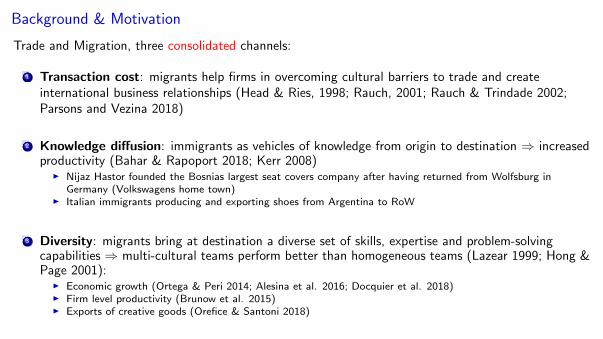
Background & Motivation
Trade and Migration, three consolidated channels:
1 Transaction cost: migrants help firms in overcoming cultural barriers to trade and createinternational business relationships (Head & Ries, 1998; Rauch, 2001; Rauch & Trindade 2002;Parsons and Vezina 2018)
2 Knowledge diffusion: immigrants as vehicles of knowledge from origin to destination ⇒ increasedproductivity (Bahar & Rapoport 2018; Kerr 2008)
I Nijaz Hastor founded the Bosnias largest seat covers company after having returned from Wolfsburg inGermany (Volkswagens home town)
I Italian immigrants producing and exporting shoes from Argentina to RoW
3 Diversity: migrants bring at destination a diverse set of skills, expertise and problem-solvingcapabilities ⇒ multi-cultural teams perform better than homogeneous teams (Lazear 1999; Hong &Page 2001):
I Economic growth (Ortega & Peri 2014; Alesina et al. 2016; Docquier et al. 2018)I Firm level productivity (Brunow et al. 2015)I Exports of creative goods (Orefice & Santoni 2018)
What do we do
Main contributions
1 Test in a unified empirical framework the three channels through which immigrants may affect theinternational competitiveness of countries: diversity, transaction costs and knowledge diffusion.
2 Dissecting the mechanism through which diversity affects the international competitiveness of sectors(heterogeneity across sectors’ characteristics)
3 Methodological contribution: improvement on the shift share IV for immigrants (based on the recentworks by Jaeger et el. 2018; Goldsmith-Pinkham et al. 2018).
4 Byproduct: Provide a new database on revealed comparative advantages.
Structure of the talk
1 Theoretical Justification
2 Descriptive evidence
3 Empirical Strategy: three channels one specificationI Data and identification strategyI Capturing the mechanismI Endogeneity
4 ResultsI Baseline (OLS and 2SLS)I Rob Check: alternative IVsI Extension: the role of skillsI Rob Check: alternative diversity index (polarization)I Rob Check: country-sector aggregated results
5 Placebo test
6 Concluding remarks
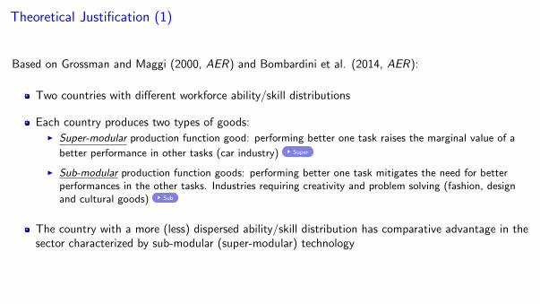
Theoretical Justification (1)
Based on Grossman and Maggi (2000, AER) and Bombardini et al. (2014, AER):
Two countries with different workforce ability/skill distributions
Each country produces two types of goods:I Super-modular production function good: performing better one task raises the marginal value of a
better performance in other tasks (car industry) Super
I Sub-modular production function goods: performing better one task mitigates the need for betterperformances in the other tasks. Industries requiring creativity and problem solving (fashion, designand cultural goods) Sub
The country with a more (less) dispersed ability/skill distribution has comparative advantage in thesector characterized by sub-modular (super-modular) technology
Theoretical Justification (2)
Immigrants coming from different origins are imperfectly substitute in production (Ottaviano andPeri 2012)
Immigrants are widely heterogeneous in their skills (positive/negative selection of migrants basedon their origin composition - Borjas (1987)
Workers from different origins are different factors of production (Ortega and Peri 2014).
Host countries with high birthplace diversity have highly disperse distribution of workerabilities/skills (workers are horizontally differentiated).
⇒ Conjecture: Birthplace Diversity is expected to improve the export performance of the hostcountries with a magnified effect in sectors requiring cognitive and problem solving capabilities.
Descriptive Evidence
510
1520
25
5 10 15 20
Transaction Costs
Exports (ln) Fitted valuesBeta: 0.91*** , N=181
510
1520
25
0 .2 .4 .6 .8 1
Birthplace Diversity
Exports (ln) Fitted valuesBeta: 4.68***, N=181
Note: Scatter plot between aggregate country specific exports and immigrant stocks are reported on the left side. Birthplace diversity and country export on the right side.
BDit ×Abstractk, interaction between birthplace diversity an the job intensity in abstract tasks.I Abstract intensity (Autor and Dorn 2013) is a dummy variable indicating whether the sector k is intensive in
complex and abstract tasks.I Rob checks: Team-Work (O*NET, Bombardini et al 2012), Complexity (Costinot 2009), Skills, Technology
(UNCTAD), Differentiated (Rauch 1999).
With a focus on the ikt specific interaction, country-year fixed effects θit can be included to reduceomitted variable concern.
Migijt, KDikt and Xijkt as in the baseline specification
Data
Bilateral stocks of migrants from UN, for a 195*195 matrix of origin-destination combinations, forthe years 1995, 2000, 2005, 2010, 2015.
I Rob Check dropping country pairs with imputed stocks
Bilateral export flows from/to 195 countries from BACI (CEPII), over the period 1995-2015,aggregated at SITC level.
Data on the presence of Preferential Trade Agreements, distance, common language, border andcolony come from CEPII databases.
Data on tariffs from WITS
Data on GDP per capita (used to calculate the remoteness measures), income and regionalclassifications are from World Bank Development Indicators data.
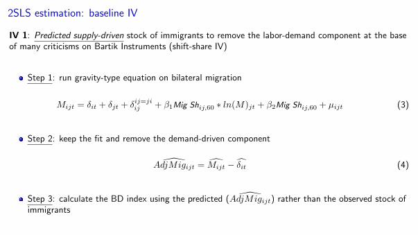
2SLS estimation: baseline IV
IV 1: Predicted supply-driven stock of immigrants to remove the labor-demand component at the baseof many criticisms on Bartik Instruments (shift-share IV)
Step 1: run gravity-type equation on bilateral migration
Step 2: keep the fit and remove the demand-driven component
AdjMigijt = Mijt − δit (4)
Step 3: calculate the BD index using the predicted ( AdjMigijt) rather than the observed stock ofimmigrants
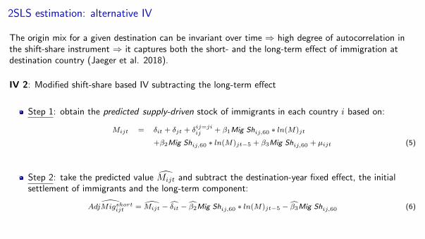
2SLS estimation: alternative IV
The origin mix for a given destination can be invariant over time ⇒ high degree of autocorrelation inthe shift-share instrument ⇒ it captures both the short- and the long-term effect of immigration atdestination country (Jaeger et al. 2018).
IV 2: Modified shift-share based IV subtracting the long-term effect
Step 1: obtain the predicted supply-driven stock of immigrants in each country i based on:
We use the time variation in AdjMigijt only from countries that experienced exogenous shock (naturaldisasters), i.e. exogenous immigrants supply shocks.
Step 1: take the predicted stock of immigrants AdjMigijt from IV 1
Step 2: use the time variation of AdjMigijt from countries experienced natural disaster in thepre-treatment period (1985-1990), i.e Ij,85−90=1
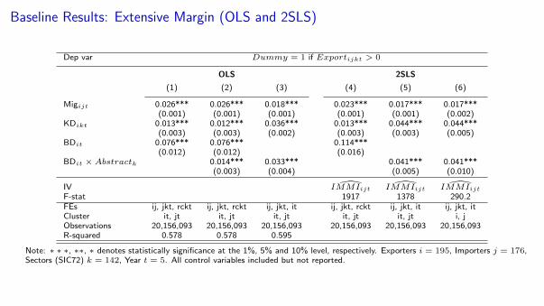
IV IMMIijt IMMIijt IMMIijtF-stat 1917 1378 290.2FEs ij, jkt, rckt ij, jkt, rckt ij, jkt, it ij, jkt, rckt ij, jkt, it ij, jkt, itCluster it, jt it, jt it, jt it, jt it, jt i, jObservations 20,156,093 20,156,093 20,156,093 20,156,093 20,156,093 20,156,093R-squared 0.578 0.578 0.595
Note: ∗ ∗ ∗, ∗∗, ∗ denotes statistically significance at the 1%, 5% and 10% level, respectively. Exporters i = 195, Importers j = 176,Sectors (SIC72) k = 142, Year t = 5. All control variables included but not reported.
IV IMMIijt IMMIijt IMMIijtF-stat 386 349.5 84.7FEs ij, jkt, rckt ij, jkt, rckt ij, jkt, it ij, jkt, rckt ij, jkt, it ij, jkt, itCluster it, jt it, jt it, jt it, jt it, jt i, jObservations 4,575,395 4,575,395 4,575,395 4,575,395 4,575,395 4,575,395R-squared 0.709 0.709 0.706
Note: ∗ ∗ ∗, ∗∗, ∗ denotes statistically significance at the 1%, 5% and 10% level, respectively. Exporters i = 195, Importers j = 176,Sectors (SIC72) k = 142, Year t = 5. All control variables included but not reported.
First Stage
Baseline by quintile in coordination cost: Intensive Margin (2SLS)Non-linear effect: BDit coefficient by bins in the average index of language dissimilarity in i
0.7
0.40.5
0.90.8
0.6
-0.4
0.0
0.4
0.8
1.2
1.6
Baseline QuintileBD 20 40 60 80 100
NOTE: Quintiles based on country-year specific average index of language dissimilarity to avoid biased calculations of quintiles due torepeated observations within it (repetitions across js)
Note: In all regressions standard errors in parentheses are double clustered at exporter and importer country level. ∗ ∗ ∗, ∗∗, ∗ denotesstatistically significance at the 1%, 5% and 10% level, respectively. Exporters i = 195, Importers j = 176, Sectors (SIC72) k = 142,Year t = 5. All control variables included but not reported.
Extension by education level of migrants. OECD, DIOC-E database
Note: ∗ ∗ ∗, ∗∗, ∗ denotes statistically significance at the 1%, 5% and 10% level, respectively. Exporters i = 114, Importers j = 174,Sectors (SIC72) k = 142, Year t = 2 (i.e. 2000, 2010). All control variables included but not reported.
Country-sector aggregate regression
1 Birthplace Diversity is country-year specific
2 Birthplace Diversity is expected to have a heterogeneous effect across sectors based on problemsolving capabilities needed in each sector k (Abstractk)
(1)+(2)⇒ Country-sector aggregated regressions for a clear-cut identification of the effect of BirthplaceDiversity on the international competitiveness of countries
Country FE Yes Yes No No NoCountry-Year FE No No Yes Yes YesSector-Year FE Yes Yes Yes Yes Yes
Note: In all regressions standard errors in parentheses are double clustered at country-sector and sector-year. ∗ ∗ ∗, ∗∗, ∗ denotes statistically significance at the 1%, 5% and 10% level,respectively. Exporters i = 186, Sectors (SIC72) k = 142, Year t = 5.
Placebo test on aggregate estimations
Diversity channel is expected to work only in sectors intensive in abstract NOT routine tasks
Observations 114,262 114,262 113,745R-squared 0.763 0.848 0.971Country-Year FE Yes Yes YesSector-Year FE Yes Yes Yes
Note: In all regressions standard errors in parentheses are double clustered at country-sector and sector-year. ∗ ∗ ∗, ∗∗, ∗ denotesstatistically significance at the 1%, 5% and 10% level, respectively. Exporters i = 186, Sectors (SIC72) k = 142, Year t = 5.
Robustness Checks
Bilateral Regression:
Team-Work Table
Polarization index Table
Country-sector aggregate:
Alternative proxies of problem solving: Table
I Team-Work (O*NET, Bombardini et al 2012)
I Complexity (Costinot 2009)
I Skill intensity in production (from UNCTAD, classification SITC 3-digit)
I Technology intensity (from UNCTAD, classification SITC 3-digit)
I Differentiated vs homogeneous goods (Rauch classification SITC 3-digit)
Sector Specific Regression Table
Concluding remarks
Diversity in the birthplace of immigrants helps the international competitiveness of the country →Migration is more than a simple positive labor supply shock
The diversity channel works on top of the transaction cost and knowledge diffusion channel
Birthplace diversity has bigger (positive) effect on problem solving intensive sectors
Bilateral Regression
Main explanatory variable: birthplace diversity index as defined in Alesina et al. (2016) and OrtegaPeri (2014), i.e. one minus the Herfindahl-Hirschman (HH) concentration index applied to thepopulation of immigrants:
BDi,t = 1−J∑
j=1
s2ijt (9)
sijt is the share of immigrants originating from j in the total population of immigrants residing incountry i at time t.
BD increases with the diversity of migrants’ birthplaces in the country (equal to 0 if there is onlyone country of origin of immigrants).
Back
Submodularity
Back
Increasing the talent of one worker reduces the marginal value of increasing the talent of the other ⇒ The two tasksare substitutable in producing the output
A reduction in the talent of one worker is compensated by a decreasing rise in the talent of the other worker
F (tA, tB) + F (t′A, t′B) ≥ F [min(tA, t
′A),min(tB , t
′B)] + F [max(tA, t
′A),max(tB , t
′B)]
Supermodularity
Back
Increasing the talent of one worker increases the marginal value of increasing the talent of the other ⇒ The twotasks are complementary in producing the output
A reduction in the talent of one worker is compensated by an increasing rise in the talent of the other worker
F (tA, tB) + F (t′A, t′B) ≤ F [min(tA, t
′A),min(tB , t
′B)] + F [max(tA, t
′A),max(tB , t
′B)]
Ex-ante measure of Comparative Advantage
Step One: run a bilateral export regression using country-sector-year (γi,k,t; γj,k,t), country-pair (γi,k,j)fixed effects, and control for Migi,j,t
Step Two: recover the exporter-sector-year fixed effects (γi,k,t) capturing all the country-sector-yearspecific determinants of international competitiveness (Costinot et al. 2012 ReSTUD)
Back
First Stage Results of baseline equation using IV 1
Dummy = 1 if Exportijkt > 0 Ln(export)|export(t−1)>0
Dep var Migijt KDikt BDit ∗ Abstractk Migijt KDikt BDit ∗ Abstractk
Controls Yes Yes Yes Yes Yes YesFEs ij, jkt, it ij, jkt, it ij, jkt, it ij, jkt, it ij, jkt, it ij, jkt, itCluster i, j i, j i, j i, j i, j i, jObservations 20,156,093 20,156,093 20,156,093 4,575,395 4,575,395 4,575,395F-test 314.2 2433.5 108.4 239.2 1811.2 207.6
Note: In all regressions standard errors in parentheses are double clustered at exporter and importer country level. ∗ ∗ ∗, ∗∗, ∗ denotes statistically significance at the 1%, 5% and 10%level, respectively. Exporters i = 195, Importers j = 176, Sectors (SIC72) k = 142, Year t = 5.
Back
Sector Specific RegressionFrench data. District-sector cross section approach on 1990 Census data and 2015 export data:
Observations 1,271 1,269 1,266 1,288 1,266 1,266R-squared 0.795 0.786 0.782 0.871 0.633 0.498Trade Year 2013 2015 2017 2017 2017 2017Region FE No No No No No YesDistrict FE Yes Yes Yes Yes Yes NoSector FE Yes Yes Yes Yes Yes Yes
Note: In all regressions standard errors in parentheses are clustered at the Region level (Region r = 22). ∗ ∗ ∗, ∗∗, ∗ denotes statistically significance at the 1%, 5% and 10% level,respectively. Districts i = 95, Sectors k = 15.
Back
Rob Check: alternative measures for problem solving intensity
Dep var RCAikt (ln)
(1) (2) (3) (4) (5) (6) (7)
BDit 0.438*** 0.440***(0.064) (0.065)
BDit*Complexityk 0.190*** 0.200***(0.040) (0.040)
BDit*Team Workk 0.162***(0.039)
BDit*Differentiatedk 0.203(0.143)
BDit*Skill Intensivek 0.613***(0.094)
BDit*High Techk 0.836***(0.143)
Observations 114,262 114,262 114,262 111,440 193,465 196,858 196,858R-squared 0.742 0.742 0.763 0.766 0.857 0.607 0.607Country FE Yes Yes No No No No NoCountry-Year FE No No Yes Yes Yes Yes YesSector-Year FE Yes Yes Yes Yes Yes Yes Yes
Note: In all regressions standard errors in parentheses are double clustered at country-sector and sector-year. ∗ ∗ ∗, ∗∗, ∗ denotes statistically significance at the 1%, 5% and 10% level,respectively. Exporters i = 186, Sectors (SITC) k = 264, Year t = 5. RTA and GDP included in column (1) and (2) when country-year fixed effects are not included.
Back
Rob Check: Polarization index as in Montalvo and Reynal-Querol (2004)
Controls Yes Yes Yes Yes Yes YesFEs ij, jkt, rckt ij, jkt, it ij, jkt, it ij, jkt, rckt ij, jkt, it ij, jkt, itCluster it, jt it, jt i, j it, jt it, jt i, jIV Migijt 0.711*** 0.640*** 0.640*** 0.589*** 0.514*** 0.514***IV KDikt 0.916*** 0.933*** 0.933*** 0.941*** 0.955*** 0.955***IV RQit 0.867*** 0.902***IV RQit ∗ Abstractk 0.893*** 0.893*** 0.918*** 0.918***F-stat 1555 1378 290.2 947.2 787.7 204.4Observations 20,156,093 20,156,093 20,156,093 4,575,395 4,575,395 4,575,395
Note: In all regressions standard errors in parentheses are double clustered at exporter and importer country level. ∗ ∗ ∗, ∗∗, ∗ denotes statistically significance at the 1%, 5% and 10%level, respectively. Exporters i = 195, Importers j = 176, Sectors (SIC72) k = 142, Year t = 5. RQit is instrumented using the predicted supply from the PPML estimation using thedistribution of foreign born residents in year 1960, as in the baseline specification.
Back
Rob Check: Team Work intensity as proxy for problem solving
Dep var Dummy = 1 if Exportijkt > 0 Ln(export)|export(t−1)>0
Controls Yes Yes Yes Yes Yes YesFEs ij, jkt, rckt ij, jkt, it ij, jkt, it ij, jkt, rckt ij, jkt, it ij, jkt, itCluster it, jt it, jt i, j it, jt it, jt i, jIV Migijt 0.640*** 0.515***IV KDikt 0.933*** 0.954***IV RQit ∗ TeamWorkk 0.895*** 0.898***F-stat 290.3 204.8Observations 19,591,612 19,591,612 19,591,612 4,501,275 4,501,275 4,501,275
Note: In all regressions standard errors in parentheses are double clustered at exporter and importer country level. ∗ ∗ ∗, ∗∗, ∗ denotesstatistically significance at the 1%, 5% and 10% level, respectively. Exporters i = 195, Importers j = 176, Sectors (SIC72) k = 138,Year t = 5. BDit is instrumented using the predicted supply from the PPML estimation using the distribution of foreign born residentsin year 1960, as in the baseline specification.


![Migration, Population Growth and Ethnic Diversity Hitotsubashi … · 2018. 11. 7. · 1995] MIGRATION, POPVLATION GROWTH AND ETHNIC DIVERSITY OF A VILLAGE IN CENTRAL ZAMBIA 99 While](https://static.documents.pub/doc/80x56/600d27b06bb3a53b0c16bd7b/migration-population-growth-and-ethnic-diversity-hitotsubashi-2018-11-7-1995.jpg)


