INTERNATIONAL ENERGY AND ENVIRONMENT thermosolar field is still ... in this chapter are some...

INTERNATIONAL

ENERGY AND ENVIRONMENT FOUNDATION

www.IEEFoundation.org

Engineering Applications of Computational Fluid Dynamics

Editor: Maher A.R. Sadiq Al-Baghdadi

Chapter **

Copyright © 2015 International Energy and Environment Foundation. All rights reserved.

CFD MODELLING IN SOLAR THERMAL ENGINEERING

M.I. Roldán1, J. Fernández-Reche

1, L. Valenzuela

1, A. Vidal

2,

E. Zarza1

1 CIEMAT-Plataforma Solar de Almería, Ctra. de Senés, km. 4.5, E04200 Tabernas,

Almería, Spain. 2 CIEMAT-Plataforma Solar de Almería, Avda. Complutense 40, Madrid E28040, Spain.

Abstract

Concentrating solar thermal technologies require complete and efficient engineering in

order to obtain the maximum performance of each facility. The thermosolar field is still

emerging, and, in many cases, the technology and facilities used are experimental.

Therefore, it is necessary to apply advanced simulation tools to predict the behaviour of the

heat transfer fluid in the solar thermal installation and to define and optimise the operating

conditions of the system.

In this sense, Computational Fluid Dynamics (CFD) is applicable to a wide range of

situations, because it is able to reproduce extreme and complex operating conditions which

are difficult to monitor. This problem may arise in any type of solar thermal facility.

Several different groups of concentrating solar thermal technologies can be defined:

medium-concentration solar technology, high-concentration solar technology, and the one

devoted to solar fuels and industrial processes at high-temperature. Each facility has its

own singularities and it may present a type of problem.

This chapter describes the application of the CFD modelling to solve design issues and to

optimise the operating conditions in different facilities belonging to the concentrating solar

thermal technologies mentioned. Simulation results led to determine both the best design of

the facility and the operating conditions optimised for each system.

For the medium-concentration technology, two cases have been analysed. One of them

studies the influence of an air gap on the temperature monitoring of absorber tubes tested in

an experimental facility installed to characterise the absorber of parabolic-trough collectors.

In the other study considered, the pressure distribution of a heat transfer fluid is evaluated

Chapter * In: Engineering Applications of Computational Fluid Dynamics. pp.***-***


2

when it is pumped through a test loop of parabolic-trough collectors in order to examine the

operating conditions of the pump.

Furthermore, a section of this chapter has been dedicated to the thermal evaluation of

volumetric receivers related to the high-concentration solar technology. In this case, the

intended aims are to predict their thermal behaviour and to determine the influence of

different operating conditions on their thermal efficiency.

Finally, the optimisation of the flow distribution in a solar reactor pre-chamber was

developed by CFD modelling in order to avoid the impact of reactive particles on a quartz

glass window located at the entrance of the reactor. This facility was built for the steam-

gasification of carbonaceous particles using concentrated solar radiation.

The studies gathered in this chapter are some examples of the CFD application in solar

thermal engineering and, as previously mentioned, the potential use of this simulation tool

is increasingly widespread in the thermosolar field. Copyright © 2015 International Energy and Environment Foundation - All rights reserved.

Keywords: CFD; Thermosolar engineering; Concentrating solar thermal technologies.

1. Introduction

Concentrating solar thermal (CST) technologies belong to an engineering field which can

significantly contribute to the delivery of clean, sustainable energy worldwide: the so-

called Solar Thermal Electricity (STE), which has been traditionally called Concentrating

Solar Power (CSP) also1 (Figure 1). It can produce electricity on demand when deployed

with thermal energy storage, providing a dispatchable source of renewable energy. Thermal

storage is relatively easy to integrate into STE technology, and allows STE plants to

smooth variability, to firm capacity and to take advantage of peak power prices. STE

generation is similar for the power block to conventional thermal generation, making STE

well fitted for hybridisation with complementary solar field and fossil fuel as primary

energy source. Moreover, CST technologies can be applied in industrial processes to

desalinise water, improve water electrolysis for hydrogen production, generate heat for

combined heat and power applications, and support enhanced oil recovery operations [1, 2].

This broad range of applications makes it necessary to improve the efficiency of the CST

technologies, which depends on direct-beam irradiation. Thus, it obtains its maximum

benefits in arid and semi-arid areas with clear skies where STE plants are installed. These

facilities use curved mirrors to concentrate solar radiation onto a receiver which absorbs the

concentrated radiation. A heat transfer fluid passes through the receiver and, for electricity

generation, it drives a turbine, converting heat into mechanical energy and then into

electricity [1].

There are four main CST technologies distinguished by the way they focus the sun’s rays

and the technology used to receive the solar energy: parabolic-trough collector (PT), solar

1 Historically CSP universally referred only to and was used in place of STE. It is only in recent years that the

term STE is becoming widespread and that some organizations moved the CSP definition to a higher level to

include both STE and CPV (Concentrating Photovoltaic). However, some organizations still use CSP to refer to

and in place of STE, and in these cases CSP does not include CPV.



3

tower (ST), linear Fresnel (LF) and parabolic dish (PD). PT and LF reflect the solar rays on

a focal line with concentration factors on the order of 60-80 and maximum achievable

temperatures of about 550°C. In PD and ST plants, mirrors concentrate the sunlight on a

single focal point with higher concentration factors (600-1,000) and operating temperatures

(800-1000°C) [3]. However, in solar tower and linear Fresnel, the receiver remains

stationary and mechanically independent from the concentrating system, which is common

for all the mirrors. In PT and PD technologies, the receiver and concentrating system move

together, enabling an optimal arrangement between concentrator and receiver regardless of

the position of the sun [1].

Figure 1. CSP technologies [1].

A detailed description of each CSP technology is included in the following sections:

Parabolic-trough collector

This is the most mature CST technology, accounting for more than 90% of the currently

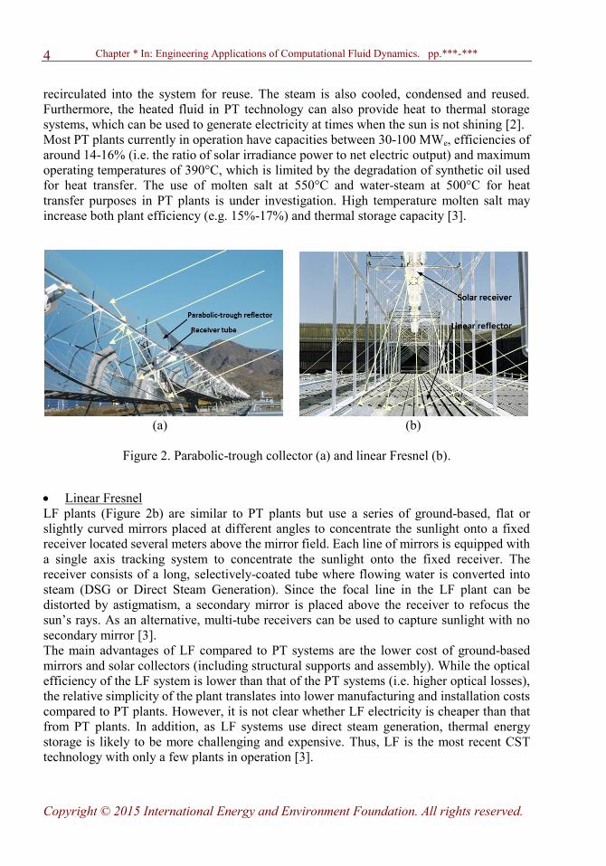
installed STE capacity worldwide. As illustrated in Figure 2, solar fields using trough

systems capture the solar radiation using large mirrors shaped like a parabola. They are

connected together in long lines of up to 300 metres and track the sun’s path throughout the

day along a single axis (usually East to West) [2, 3].

The parabolic mirrors send the solar beam onto a receiver pipe which is located at the focal

line of the parabola and filled with a specialised heat transfer fluid. These receivers have a

special coating to maximise energy absorption and minimise infrared re-irradiation. In

order to avoid convection heat losses, the pipes work in an evacuated glass envelope.

The thermal energy is removed by the heat transfer fluid (e.g. synthetic oil, molten salt)

flowing in the heat-absorbing pipe and transferred to a steam generator to produce the

super-heated steam that drives the turbine [3]. Once the fluid transfers its heat, it is



4

recirculated into the system for reuse. The steam is also cooled, condensed and reused.

Furthermore, the heated fluid in PT technology can also provide heat to thermal storage

systems, which can be used to generate electricity at times when the sun is not shining [2].

Most PT plants currently in operation have capacities between 30-100 MWe, efficiencies of

around 14-16% (i.e. the ratio of solar irradiance power to net electric output) and maximum

operating temperatures of 390°C, which is limited by the degradation of synthetic oil used

for heat transfer. The use of molten salt at 550°C and water-steam at 500°C for heat

transfer purposes in PT plants is under investigation. High temperature molten salt may

increase both plant efficiency (e.g. 15%-17%) and thermal storage capacity [3].

(a) (b)

Figure 2. Parabolic-trough collector (a) and linear Fresnel (b).

Linear Fresnel

LF plants (Figure 2b) are similar to PT plants but use a series of ground-based, flat or

slightly curved mirrors placed at different angles to concentrate the sunlight onto a fixed

receiver located several meters above the mirror field. Each line of mirrors is equipped with

a single axis tracking system to concentrate the sunlight onto the fixed receiver. The

receiver consists of a long, selectively-coated tube where flowing water is converted into

steam (DSG or Direct Steam Generation). Since the focal line in the LF plant can be

distorted by astigmatism, a secondary mirror is placed above the receiver to refocus the

sun’s rays. As an alternative, multi-tube receivers can be used to capture sunlight with no

secondary mirror [3].

The main advantages of LF compared to PT systems are the lower cost of ground-based

mirrors and solar collectors (including structural supports and assembly). While the optical

efficiency of the LF system is lower than that of the PT systems (i.e. higher optical losses),

the relative simplicity of the plant translates into lower manufacturing and installation costs

compared to PT plants. However, it is not clear whether LF electricity is cheaper than that

from PT plants. In addition, as LF systems use direct steam generation, thermal energy

storage is likely to be more challenging and expensive. Thus, LF is the most recent CST

technology with only a few plants in operation [3].



5

Solar tower

In the ST plants (Figure 3a), also called central receiver systems (CRS) or power tower, a

large number of computer-assisted mirrors (heliostats) track the sun individually over two

axes and concentrate the solar radiation onto a single receiver at the top of a central tower

where the solar heat drives a thermodynamic cycle and generates electricity. ST plants can

achieve higher temperatures than PT and LF systems because they have higher

concentration factors. The CRS can use water-steam (DSG) or molten salt as the primary

heat transfer fluid. The use of high-temperature gas is also being considered (e.g.

atmospheric or pressurised air in volumetric receivers) [3].

In a direct steam ST, water is pumped up the tower to the receiver, where concentrated

thermal energy heats it to around 550°C. The hot steam then powers a conventional steam

turbine [2]. When DSG is used as heat transfer fluid, it is not required a heat exchanger

between the primary transfer fluid and the steam cycle, but the thermal storage is more

difficult.

Depending on the primary heat transfer fluid and the receiver design, maximum operating

temperatures may range from 250-300°C (using water-saturated steam) and up to 565°C

(using molten salt and water-superheated steam). Temperatures above 800°C can be

obtained using gases (e.g. atmospheric air). Thus, the temperature level of the primary heat

transfer fluid determines the operating conditions (i.e. subcritical, supercritical or ultra-

supercritical) of the steam cycle in the conventional part of the power plant.

ST plants can be equipped with thermal storage systems whose operating temperatures also

depend on the primary heat transfer fluid. Today’s best performance is obtained using

molten salt at 565°C for both heat transfer and storage purposes. This enables efficient and

cheap heat storage and the use of efficient supercritical steam cycles [3].

High-temperature ST plants offer potential advantages over other CST technologies in

terms of efficiency, heat storage, performance, capacity factors and costs. In the long run,

they could provide the cheapest STE, but more commercial experience is needed to confirm

these expectations. However, a large ST plant can require thousands of computer-

controlled heliostats, that move to maintain point focus with the central tower from dawn to

dusk, and they typically constitute about 50% of the plant’s cost.

Current installed capacity includes ST plant size of around 11 MW and 20 MW for

water/saturated steam (e.g. PS10 and PS20 commercial projects in Spain) and 120 MW for

water/superheated steam (e.g., IVANPAH project in EEUU with 360 MW distributed in

three different solar towers). Larger ST plants have expansive solar fields with a high

number of heliostats and a greater distance between them and the central receiver. This

results in more optical losses, atmospheric absorption and angular deviation due to mirror

and sun-tracking imperfections. Therefore, ST still has room for improvement of its

technology [2, 3].

Parabolic dish

The PD system (Figure 3b) consists of a parabolic dish shaped concentrator that reflects

sunlight into a receiver placed at the focal point of the dish. The receiver may be a Stirling

engine or a micro-turbine. PD systems require two-axis sun tracking systems and offer very

high concentration factors and operating temperatures. The main advantages of PD systems

include high efficiency (i.e. up to 30%) and modularity (i.e. 3-50 kW), which is suitable for



6

distributed generation. Unlike other STE options, PD systems do not need cooling systems

for the exhaust heat. This makes PDs suitable for use in water-constrained regions, though

at relatively high electricity generation costs compared to other CST technologies.

However, the PD system is still under demonstration and investment costs are still high [3].

(a) (b)

Figure 3. Solar tower (a) and parabolic dish (b).

As previously mentioned, more than 90% of the installed STE capacity in 2014 consisted

of PT plants; ST plants total about 170 MW and LF plants about 40 MW. A comparison of

CST technology performance is shown in Table 1 [3].

Table 1. Performance of CST technologies [4-6].

PT PT PT ST ST ST LF PD

Storage no yes yes no/yes no/yes yes no no

Status comm comm demo demo comm demo demo demo

Capacity [MW] 15-80 50-280 5 10-20 50-370 20 5-30 0.025

HT fluid oil oil salt steam steam salt sat. st na

HTF temp [ºC] 390 390 550 250 565 565 250 750

Storage fluid no salt salt steam na salt no no

Storage time [h] 0 7 6-8 0.5-1 na 15 0 0

Storage temp [ºC] na 380 550 250 na 550 na na

Efficiency [%] 14 14 14/16 14 16 15/19 11/13 25/30

Cap. factor [%] 25-28 29-43 29-43 25-28 25-28 55-70 22-24 25-28

Optical efficiency H H H M M H L VH

Concentration 70-80 70-80 70-80 1000 1000 1000 60-70 >1300

Land [ha/MW] 2 3 2 2 2 2 2 na

Cycle sh. st sh. st sh. st sat. st sh. st sh. st sat. st na

Cycle temp [ºC] 380 380 540 250 540 540 250 na

Grid on on on on on on on on/off

sat. st=satured steam; sh. st=superheated steam; L=low; M=middle; H=high; VH=very high

na=not applicable



7

So far, linear-Fresnel and parabolic dish systems are starting to commercially develop, and

parabolic trough and solar tower account for the vast majority of operational STE capacity,

despite the fact that these technologies reach a medium solar-to-electricity efficiency.

Therefore, innovations in this field must provide a reliable, efficient and cost-competitive

technology.

In this sense, STE engineering is focused on optimising the thermal energy conversion

cycle and thermal storage. Innovations in CST technologies must increase efficiency by

using advanced optical components and systems operating at higher temperatures, and

improve dispatchability by deploying advanced thermal storage and hybridisation concepts.

New heat transfer fluids such as gases and molten salts are proposed to be used in CST

plants, together with the introduction of dry cooling designs to limit the water consumption

and reduce the environmental footprint of solar operations [1, 2].

Next sections in this chapter describe the application of the CFD modelling to solve design

issues and to optimise the operating conditions in different facilities belonging to the

concentrating solar thermal technologies mentioned. Simulation results led to determine

both the best design of the facility and the operating conditions optimised for each system.

2. Medium-concentration solar technology

This section focuses on the analysis of issues found in two experimental facilities installed

to test and characterise components for parabolic-troughs (PT) solar fields. These systems

belong to medium-concentration solar technology.

2.1 Thermal analysis of a characterisation chamber for absorber tubes used in parabolic-

trough collectors

As previously mentioned, PT collectors consist of a reflector and an absorber tube where

the solar radiation is collected. In order to characterise the absorber, a test chamber has

been designed and installed at laboratory scale. The CFD study analysed the thermal

behaviour of the test bed, so as to determine the influence of an air gap on the heat transfer

between the constituent elements of the test facility.

Facility description and procedure

The characterisation of different absorber tubes for PT collectors is based on the analysis of

their thermal map when they receive the thermal energy from a constant heat source. In

order to study this characterisation process, an experimental facility has been installed.

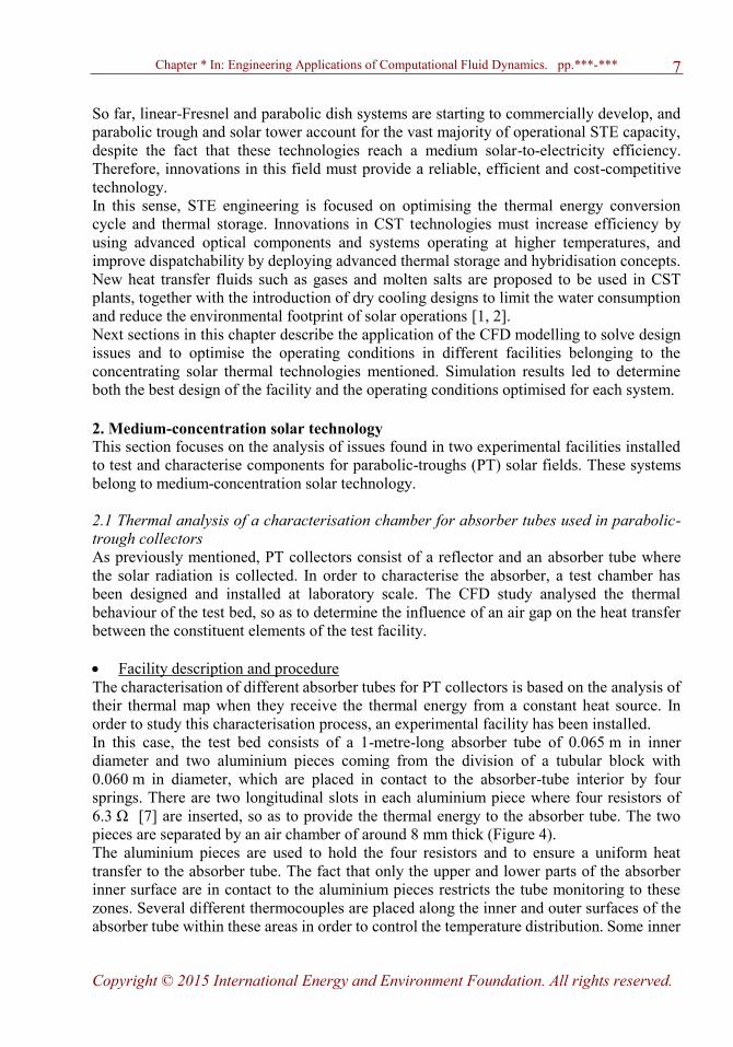
In this case, the test bed consists of a 1-metre-long absorber tube of 0.065 m in inner

diameter and two aluminium pieces coming from the division of a tubular block with

0.060 m in diameter, which are placed in contact to the absorber-tube interior by four

springs. There are two longitudinal slots in each aluminium piece where four resistors of

6.3 Ω [7] are inserted, so as to provide the thermal energy to the absorber tube. The two

pieces are separated by an air chamber of around 8 mm thick (Figure 4).

The aluminium pieces are used to hold the four resistors and to ensure a uniform heat

transfer to the absorber tube. The fact that only the upper and lower parts of the absorber

inner surface are in contact to the aluminium pieces restricts the tube monitoring to these

zones. Several different thermocouples are placed along the inner and outer surfaces of the

absorber tube within these areas in order to control the temperature distribution. Some inner



8

thermocouples have been bent to ensure that their tips are in contact with the absorber inner

surface and others have been welded to a small steel plate to increase the contact surface

between their tip and the absorber inner surface. The outer thermocouples have been

flanged and electrowelded.

Figure 4. Characterisation device for absorber tubes.

Preliminary results showed a temperature difference between inner and outer surfaces of

around 40ºC and a thermal gradient of 30ºC between two different points of the outer

surface. These high temperature differences are in disagreement with basic heat transfer

equations if a good thermal contact existed between the aluminium pieces and the inner

surface of the absorber tube. In order to determine the source of this problem, several

different CFD simulations were developed considering various configurations that took into

account the existence of an air gap between the inner surface of the absorber tube and the

aluminium pieces (Table 2).

Firstly, the ideal case without air gap was compared with a real one considering an air gap

of 1 mm between the aluminium piece and the absorber tube but both elements maintained

their connection in the upper and lower parts. After this evaluation, the two configurations

with a greater air gap were studied, as so to determine the influence of the air gap on the

heat transfer to the absorber.

In all cases, the boundary conditions were obtained from the steady state of one test, which

are collected in Table3.

Numerical modelling

The simulation domain consists of a three-dimensional geometry that represents a part of

the absorber tube whose front and back surfaces are the cross sections. The subdomains

defined in the ideal case are included in Figure 4. If there is an air gap between the



9

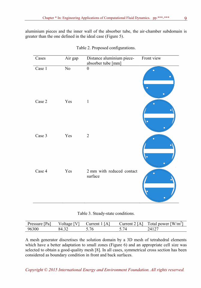
aluminium pieces and the inner wall of the absorber tube, the air-chamber subdomain is

greater than the one defined in the ideal case (Figure 5).

Table 2. Proposed configurations.

Cases Air gap Distance aluminium piece-

absorber tube [mm]

Front view

Case 1 No 0

Case 2 Yes 1

Case 3 Yes 2

Case 4 Yes 2 mm with reduced contact

surface

Table 3. Steady-state conditions.

Pressure [Pa] Voltage [V] Current 1 [A] Current 2 [A] Total power [W/m2]

96300 84.32 5.76 5.74 24127

A mesh generator discretises the solution domain by a 3D mesh of tetrahedral elements

which have a better adaptation to small zones (Figure 6) and an appropriate cell size was

selected to obtain a good-quality mesh [8]. In all cases, symmetrical cross section has been

considered as boundary condition in front and back surfaces.



10

Figure 5. Simulation domain with air gap.

Figure 6. Mesh and boundary conditions.

The CFD model involves solving the continuity (1), momentum (2) [9] and energy (3) [10]

equations because the dynamical behaviour of a fluid is determined by the conservation

laws [11].

mSvt

(1)



11

Fgpvvv

t )( (2)

h

j

effjjeff SvJhTkpEvEt

(3)

where is the density of the fluid (kg/m3), t is elapsed time (s),

v is the velocity vector

with respect to the 3D coordinate system (m/s), Sm is the mass source (kg/s m3), p is the

static pressure (Pa), is the stress tensor (N/m2), ·

g is the gravitational body force,

F

is the external body force (N/m3), E is the energy transfer (

2

2vphE

) (J/kg), keff is

the effective conductivity which includes the turbulence thermal conductivity (W/m K), hj

is the enthalpy of species j (J/kg),

jJ is the diffusion flux of species j (kg/s m2), eff is the

viscous stress tensor (N/m2) and Sh is the volumetric heat source (W/m

3). These general

equations take into account the three dimensions and, in this case, the air is the only species

involved in the fluid medium.

The operating pressure was set to 96300 Pa and the heat is mainly transferred from the

aluminium pieces to the absorber tube by conduction with losses due to free convection.

Furthermore, it is assumed that the fluid is under steady-state flow condition and a free

convection is considered between the outer wall of the absorber tube and the ambient air

taking into account a convection coefficient of 17.5 W/m2 K [12]. In order to consider the

influence of the gravitational force on the air confined between the aluminium piece and

the absorber tube, the turbulence model “κ-ε renormalization group” was selected to

simulate flow regimes with low Reynolds number [10].

The boundary conditions considered in the CFD model were: symmetry condition for the

front and back cross surfaces, free convection for the outer wall with a heat transfer

coefficient of 17.5 W/m2 K and a fluid temperature of 300 K, heat flux of 24127 W/m

2

(Table 3) for the walls next to the resistors, and the remaining inner walls were coupled to

adjacent zones.

The thermophysical properties of the fluid (dry air) are described by the following

equations, where the temperature (T) must be considered in K [13]:

)0009658.0()006611.0( 9227.0565.3 TT ee (4)

4103072 ·10·973.1·10·349.8·001189.0·4692.01064 TTTTc p

(5)

4.110

10·458.1 2/36

T

T (6)



12

31228 ·10·66.7·10·594.3·00007502.000647.0 TTT (7)

where ρ is the air density (kg/m

3), cp is the specific heat capacity (J/kg K), μ is the dynamic

viscosity (kg/m s), and λ is the thermal conductivity (W/m K).

The aluminium density is 2719 kg/m3, its specific heat capacity is 871 J/kg K, and a

thermal conductivity of 202.4 W/m K has been considered for the operating temperature

range. The density of the ferritic steel was set to 7763 kg/m3, its thermal conductivity fixed

was 38 W/m K, and its specific heat capacity is defined by:

2·000573.0·2368.01.503 TTc p (8)

where T is the temperature in K.

Results

For the purpose of evaluating the influence of an air gap on the heat transfer between the

aluminium pieces heated by resistors and the absorber tube of a PT collector, an ideal

configuration with a full contact between the aluminium piece and the absorber tube was

compared to different real configurations with air gaps of 1 and 2 mm thick using CFD

simulation.

The thermal distribution at the central section of the domain was obtained for both cases

and it was observed that the temperature variation in the case of 1-mm air gap was around

12 K, whereas the temperature variation is practically negligible (2 K) in the ideal case.

Both thermal profiles have been depicted in Figure 7.

(a)



13

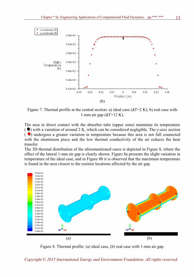
(b)

Figure 7. Thermal profile at the central section: a) ideal case (ΔT=2 K), b) real case with

1-mm air gap (ΔT=12 K).

The area in direct contact with the absorber tube (upper zone) maintains its temperature

( ) with a variation of around 2 K, which can be considered negligible. The y-axis section

( ) undergoes a greater variation in temperature because this area is not full connected

with the aluminium piece and the low thermal conductivity of the air reduces the heat

transfer.

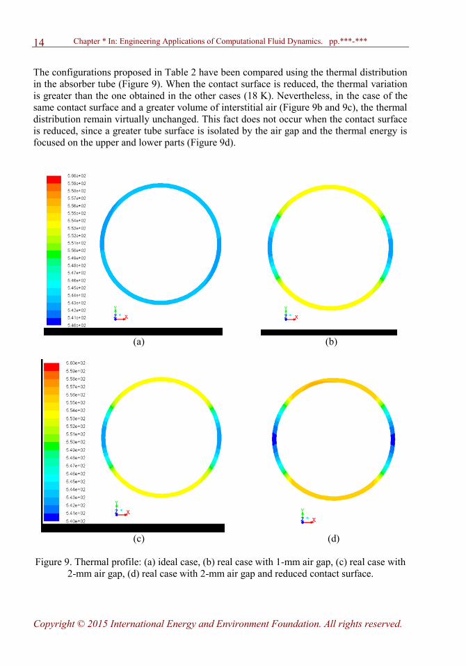
The 3D thermal distribution of the aforementioned cases is depicted in Figure 8, where the

effect of the lateral 1-mm air gap is clearly shown. Figure 8a presents the slight variation in

temperature of the ideal case, and in Figure 8b it is observed that the maximum temperature

is found in the area closest to the resistor locations affected by the air gap.

(a) (b)

Figure 8. Thermal profile: (a) ideal case, (b) real case with 1-mm air gap.



14

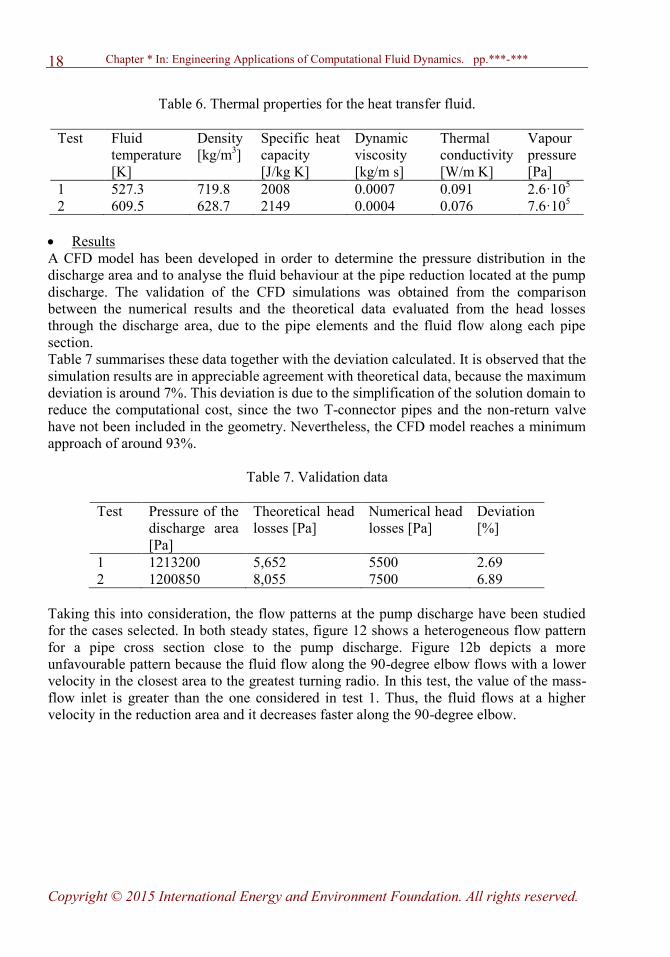
The configurations proposed in Table 2 have been compared using the thermal distribution

in the absorber tube (Figure 9). When the contact surface is reduced, the thermal variation

is greater than the one obtained in the other cases (18 K). Nevertheless, in the case of the

same contact surface and a greater volume of interstitial air (Figure 9b and 9c), the thermal

distribution remain virtually unchanged. This fact does not occur when the contact surface

is reduced, since a greater tube surface is isolated by the air gap and the thermal energy is

focused on the upper and lower parts (Figure 9d).

(a) (b)

(c) (d)

Figure 9. Thermal profile: (a) ideal case, (b) real case with 1-mm air gap, (c) real case with

2-mm air gap, (d) real case with 2-mm air gap and reduced contact surface.



15

Summary and conclusions

The study described above was developed to determine the influence of an air gap on the

heat transfer between the constituent elements of a test bed to characterise absorber tubes

used in PT collectors. For that purpose, different configurations were considered in the

CFD analysis whose results are collected in Table 4.

Table 4. Temperature range reached by the absorber tube

Case Temperature range in

the absorber tube, [K]

Variation in temperature

of the absorber tube, [K]

1 542-544 2

2 542-553 9

3 543-553 10

4 539-558 19

Numerical results show that the ideal case (1), without air gap, maintains virtually a

homogeneous thermal profile, whereas the configuration with 1-mm air gap presents a

variation of around 10 K. Furthermore, the smaller the contact surface between the

absorber tube and the aluminium piece, the greater variation in temperature the absorber

tube presents.

The temperature distributions obtained demonstrate that the air gap acts as a barrier to heat

transfer between the aluminium piece and the absorber tube, obtaining a maximum

temperature in the area closest to the resistor locations affected by the air gap. As a

consequence, the test bed used to characterise the absorber tube must reach a full contact

between the piece which transfers the energy supplied by the heat source and the absorber

tube tested. Otherwise, the characterisation of the absorber tube cannot be developed by a

reliable methodology.

2.2 Pressure distribution of a heat transfer fluid pumped through a test loop of parabolic-

trough collectors

A test loop of PT collectors was built to study new prototypes of PT collectors and

configuration of the solar fields [14]. The start-up of the facility requires a proper operation

of the pump that drives the heat transfer fluid (Syltherm 800) along the pipes. Thus, a CFD

analysis was used to determine the pressure distribution of a section from the suction area

and to study the appropriateness of the operating conditions.

Facility description and procedure

In order to obtain the discharge pressure of the pump, a CFD simulation has been

developed considering a section of the discharge side with a pipe reduction after the pump

outlet, a non-return valve, two T-connector pipes, a 90-degree elbow and three pipe

lengths. Figure 10 shows the location of the elements mentioned.



16

Figure 10. Description of the discharge section selected.

The CFD model has been developed to determine the fluid behaviour in the pipe reduction

of the pump outlet and to obtain the discharge pressure. The boundary conditions were

selected from the steady state of two tests and the model was validated using the pressure

drop produced in each pipe section (Table 5).

Table 5. Steady-state conditions for each test.

Test Fluid

temperature [K]

Suction

pressure [Pa]

Discharge

pressure [Pa]

Mass flow

[kg/s]

1

2

527.3

609.5

1.14·106

1.12·106

1.21·106

1.20·106

6.92

7.22

Numerical modelling

In this case, the three-dimensional solution domain is the fluid (Figure 10), because the

pipe wall is insulated and considered as adiabatic wall. The mesh selected consists of

208140 tetrahedral cells with a minimum orthogonal quality of 0.5 (Figure 11). This

parameter determines the skew of a cell. Thus, its value is 0 when the cell has a bad quality

and it is 1 for high-quality cells.



17

Figure 11. Mesh and boundary conditions.

The dynamical behaviour of a fluid is determined by the conservation laws (conservation of

mass, momentum, and energy). Therefore, the CFD model requires solving the continuity,

momentum and energy equations described in section 2.1. It is considered that the fluid

flows at a constant temperature fixed by the steady state selected and, so as to analyse the

fluid flow through the pipe section, the turbulence model “κ-ε renormalization group” was

selected because it regards flow regimes with low Reynolds number [10].

The boundary conditions are shown in Figure 11, where the outer wall is considered an

adiabatic one because it is insulated. Gauge pressure, fluid temperature and mass-flow inlet

at the steady state were fixed as boundary conditions.

The pipes of the facility consist of steel (AISI 316) with a density of 7980 kg/m3, its

specific heat capacity is 500 J/kg K, and its thermal conductivity is 15 W/m K. The thermal

properties of the fluid (Syltherm 800) were obtained for the fluid temperature of each

steady state (Table 6).



18

Table 6. Thermal properties for the heat transfer fluid.

Test Fluid

temperature

[K]

Density

[kg/m3]

Specific heat

capacity

[J/kg K]

Dynamic

viscosity

[kg/m s]

Thermal

conductivity

[W/m K]

Vapour

pressure

[Pa]

1

2

527.3

609.5

719.8

628.7

2008

2149

0.0007

0.0004

0.091

0.076

2.6·105

7.6·105

Results

A CFD model has been developed in order to determine the pressure distribution in the

discharge area and to analyse the fluid behaviour at the pipe reduction located at the pump

discharge. The validation of the CFD simulations was obtained from the comparison

between the numerical results and the theoretical data evaluated from the head losses

through the discharge area, due to the pipe elements and the fluid flow along each pipe

section.

Table 7 summarises these data together with the deviation calculated. It is observed that the

simulation results are in appreciable agreement with theoretical data, because the maximum

deviation is around 7%. This deviation is due to the simplification of the solution domain to

reduce the computational cost, since the two T-connector pipes and the non-return valve

have not been included in the geometry. Nevertheless, the CFD model reaches a minimum

approach of around 93%.

Table 7. Validation data

Test Pressure of the

discharge area

[Pa]

Theoretical head

losses [Pa]

Numerical head

losses [Pa]

Deviation

[%]

1

2

1213200

1200850

5,652

8,055

5500

7500

2.69

6.89

Taking this into consideration, the flow patterns at the pump discharge have been studied

for the cases selected. In both steady states, figure 12 shows a heterogeneous flow pattern

for a pipe cross section close to the pump discharge. Figure 12b depicts a more

unfavourable pattern because the fluid flow along the 90-degree elbow flows with a lower

velocity in the closest area to the greatest turning radio. In this test, the value of the mass-

flow inlet is greater than the one considered in test 1. Thus, the fluid flows at a higher

velocity in the reduction area and it decreases faster along the 90-degree elbow.



19

(a)

(b)

Figure 12. Velocity distribution at the pipe reduction: (a) test 1, (b) test 2.

The previous velocity distribution corresponds to the pressure one depicted in Figure 13. In

both cases, the maximum pressure is located in the pipe section that connects the pump

discharge with the pipe reduction. Nevertheless, the minimum pressure is located at the

beginning of the pipe reduction, after the area of the maximum pressure. This causes the

lack of homogeneity in the fluid flow of the discharge area. In the remaining part of the

pipe domain, the pressure distribution is virtually homogeneous.



20

(a) (b)

Figure 13. Pressure distribution at the pipe reduction: (a) test 1, (b) test 2.

Summary and conclusions

It is required to study the fluid behaviour in a pipe reduction located at the pump discharge

of a PT facility. For that purpose, a CFD model has been developed in order to determine

the pressure and velocity distributions for a pipe section selected from the discharge area.

The boundary conditions of the simulations have been obtained from an experimental

steady state selected for each test regarded. Simulation results demonstrate that the CFD

model presents a maximum deviation of around 7% with respect to the experimental data,

due to the simplification applied to the geometry of the simulation domain.

Regarding this approach, the analysis of the flow pattern obtained shows a great velocity

variation in a pipe cross section close to the pump discharge. Furthermore, the maximum

pressure is located in the pipe section that connects the pump discharge with the pipe

reduction. In contrast to this, the minimum pressure is found directly after the area of the

maximum pressure. The fact that these extreme conditions occur in connected areas may

produce an undesirable effect on the fluid flow.

3. High-concentration solar technology

The thermal behaviour of solar receivers is a key issue for the improvement of thermal

efficiency in ST plants. Therefore, in this section, it is summarised the procedure followed

for the analysis of a metallic volumetric receiver in a test facility.

Volumetric solar receivers are thermal systems, in which concentrated solar radiation is

absorbed on the surface of a material, which transfers the heat to a working fluid. The



21

absorbed heat is transferred when the fluid passes through a porous medium. In this case,

the heat transfer fluid is air and the porous medium is a metallic material.

3.1 Facility description and procedure

The prediction of the fluid-dynamic behaviour in solar volumetric receivers allows

optimising their design and improving their thermal efficiency. Therefore, the thermal

behaviour of a tested volumetric receiver was analysed by a CFD model. The validation of

the simulations leads to establish a prediction procedure that also enables the study of the

receiver behaviour under any operating conditions.

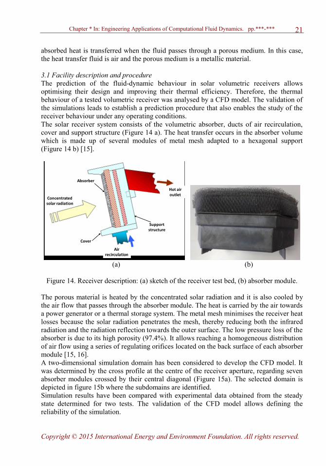
The solar receiver system consists of the volumetric absorber, ducts of air recirculation,

cover and support structure (Figure 14 a). The heat transfer occurs in the absorber volume

which is made up of several modules of metal mesh adapted to a hexagonal support

(Figure 14 b) [15].

(a) (b)

Figure 14. Receiver description: (a) sketch of the receiver test bed, (b) absorber module.

The porous material is heated by the concentrated solar radiation and it is also cooled by

the air flow that passes through the absorber module. The heat is carried by the air towards

a power generator or a thermal storage system. The metal mesh minimises the receiver heat

losses because the solar radiation penetrates the mesh, thereby reducing both the infrared

radiation and the radiation reflection towards the outer surface. The low pressure loss of the

absorber is due to its high porosity (97.4%). It allows reaching a homogeneous distribution

of air flow using a series of regulating orifices located on the back surface of each absorber

module [15, 16].

A two-dimensional simulation domain has been considered to develop the CFD model. It

was determined by the cross profile at the centre of the receiver aperture, regarding seven

absorber modules crossed by their central diagonal (Figure 15a). The selected domain is

depicted in figure 15b where the subdomains are identified.

Simulation results have been compared with experimental data obtained from the steady

state determined for two tests. The validation of the CFD model allows defining the

reliability of the simulation.



22

(a)

(b)

Figure 15. Definition of the two-dimensional geometry.

Table 8 summarises the steady-state conditions for the two tests considered. The incoming

heat flux was obtained by the indirect flux measuring system [17].

Table 8. Steady-state conditions.

Test Pressure

[Pa]

Air mass-flow

[kg/s]

Wind velocity

[m/s]

Wind

direction [º]

Total power

received [kW]

1

2

97680

97680

2.72

3.45

3.60

3.30

142.49

268.50

2405.03

2811.54

3.2 Numerical modelling

The solution domain consists of seven absorber modules located at the central cross section

of the receiver, the area of the recirculation air and the ambient air. Each module has two



23

subdomains: the porous material and the hot air (Figure 15b). The mesh selected is made up

of quadrilateral cells (structured grid) with an equiangle skew (QEAS) of 0.4 and a maximum

aspect ratio (QAR) of 1.28. These parameters inform about the mesh quality (QEAS) and the

cell deviation from the equilateral shape (QAR). The 100% of the cells are in the QEAS range

0-0.4 which corresponds to the excellent (0-0.25) and good (0.25-0.5) quality [8]. The

maximum QAR is 1.28 that is close to 1, thus there is a slight deviation from the equilateral

shape. Figure 16 shows the adaptation of the mesh selected to the geometry.

Figure 16. Mesh and boundary conditions of the solution domain.

The CFD model takes into account the conservation laws by the equations (1), (2) and (3)

defined in section 2.1. Furthermore, it is assumed a steady-state flow condition for the fluid

(air). Therefore, an experimental quasi-steady state from each test considered was defined

in order to determine the operating conditions (table 8). The viscous model selected was “κ-ε renormalization group” because the Reynolds number evaluated at the absorber outlet for

the temperature range of 900-1000 K and considering an experimental mass flow of

0.025 kg/s is low and this turbulence model accounts for Reynolds-number effects in this

range [10].

The gravitational force was neglected because of the low density of the air, the forced air

stream and the horizontal position of the receiver. Nevertheless, forced convection has been

regarded for the outer and inner walls of each absorber module, using an average heat

transfer coefficient of 165 W/m2 K for air forced convection (coefficient range between

30 W/m2 K and 300 W/m

2 K [12]).

The volumetric heat source was defined following an exponential law that is an approach of

the radiation-intensity attenuation in the absorber material. This phenomenon was

described for 2D by the following equation [18, 19]:

yeIyI

0)( (9)

where I is the intensity of the solar radiation which goes through the absorber

depth (W/m3), ξ is the optical extinction coefficient (m

-1), y is the position in y-axis



24

direction (m), and I0 is the initial intensity of the solar radiation (W/m3) which depends on

the incoming superficial heat flux (IS0) and ξ [19]:

00 SII (10)

In order to calculate ξ, the metal mesh of the absorber has been considered as a structure of

parallel cylinders and the scattering has been neglected. Thereby, ξ can be evaluated

by [20]:

)1(

cos

41ln

1)( Po

dH (11)

where dH is the hydraulic diameter obtained from the average diameter of the pores in the

metal mesh, γ is the incidence angle of the radiation which depends on the heliostat position

with respect to the focus location, and Po is the porosity. Thus, for each test, the volumetric

heat source has been implemented as user defined function (UDF) using the following

expressions (Table 9).

Table 9. Equations for the volumetric heat source.

Test Volumetric heat source [W/m3]

1

2

y

v eQ 59.215718975

y

v eQ 59.216685775

The metal mesh of each absorber module is regarded as a porous material with a viscous

loss term of 3.02·107 m

-2 and an inertial loss term of 25.45 m

-1 in the flow direction (0,-1).

For the secondary flow direction, the resistance to the fluid flow is neglected; thereby it is

considered a much greater value of these terms (1010

m-2

and 1000 m-1

, respectively) in the

flow direction (1,0).

Figure 16 shows the boundary conditions selected. The inlet velocity of the ambient air was

obtained from the mass flow measured in the flow direction (0,-1) at ambient temperature

(about 295 K). The inlet velocity of the wind was measured together with its incidence

angle at the ambient temperature. Both air and wind outlets were defined jointly as outflow.

The inlet velocity of the recirculation air has been calculated taking into account the inlet

area, its density at the inlet temperature (about 520 K) and the recirculation rate (ARR) that

is evaluated from the air mass flow (ma) by the following equation [15]:

airmARR )011.0(082.0)03.0(26.0 (12)

The walls that delimit the porous medium were defined by a porous-jump condition. This

case require to include the material permeability (3.314·10-8

m2) and the pressure-jump

coefficient (508.82 m-1

). The outer walls of the absorber module are defined considering



25

force convection with a heat transfer coefficient of 165 W/m2 K and the temperature range

of the hot air. The remaining walls are coupled to the adjacent areas.

The absorber material is a metallic alloy with a density of 8110 kg/m3, a thermal

conductivity of 24 W/m K and its specific heat capacity is defined by a temperature-

dependent piecewise linear profile [21]. The alloy used in the support structure has a

density of 8000 kg/m3, a thermal conductivity of 23.6 W/m K and its specific heat capacity

is also determined by a piecewise linear profile [22]. The thermophysical properties of the

fluid (dry air) have been described in section 2.1.

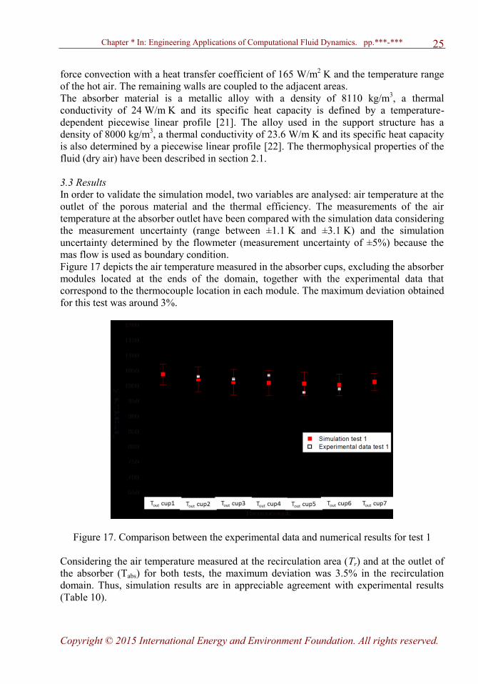
3.3 Results

In order to validate the simulation model, two variables are analysed: air temperature at the

outlet of the porous material and the thermal efficiency. The measurements of the air

temperature at the absorber outlet have been compared with the simulation data considering

the measurement uncertainty (range between ±1.1 K and ±3.1 K) and the simulation

uncertainty determined by the flowmeter (measurement uncertainty of ±5%) because the

mas flow is used as boundary condition.

Figure 17 depicts the air temperature measured in the absorber cups, excluding the absorber

modules located at the ends of the domain, together with the experimental data that

correspond to the thermocouple location in each module. The maximum deviation obtained

for this test was around 3%.

Figure 17. Comparison between the experimental data and numerical results for test 1

Considering the air temperature measured at the recirculation area (Tr) and at the outlet of

the absorber (Tabs) for both tests, the maximum deviation was 3.5% in the recirculation

domain. Thus, simulation results are in appreciable agreement with experimental results

(Table 10).



26

Table 10. Deviation between experimental data and simulation results.

Test (Tabs)exp

[K]

(Tabs)sim

[K]

Deviation

[%]

(Tr)exp

[K]

(Tr)sim

[K]

Deviation

[%]

1

2

981.7

997.0

1014.7

1003.8

3.36

0.68

380.1

369.8

381.9

363.5

0.47

1.71

The thermal distribution simulated for test 1 is depicted in Figure 18, where the ambient air

increases its temperature due to the effect of the recirculation air and it is reached a lower

air temperature in the areas influenced by the wind.

Figure 18. Thermal distribution obtained for test 1.

The thermal efficiency achieved was evaluated by the following equation [23]:

rec

conv

Q

Q (13)

where η is the thermal efficiency of the receiver, and Qconv is the convective flow obtained

from the energy balance between the fluid inlet and the absorber outlet (W):

Qconv = mf · cpf · (Tf,out - Tf,in) (14)

where mf is the air mass flow that passes through the absorber modules (kg/s), cpf is the

average specific heat capacity of the air (J/kg K), Tf,in is the air temperature at the absorber

inlet (K), and Tf,out is the air temperature at the outlet of the absorber module (K).

Qrec is the heat absorbed from the incoming concentrated solar radiation over the inlet

receiver surface (W), whose evaluation considers the superficial heat source (IS0, W/m2)

according to the frontal receiving area of 7.07 m2 (A).



27

Qrec = IS0·A (15)

Table 11 summarises the thermal efficiency of the receiver obtained from experimental and

simulation results. Their comparison shows a maximum deviation of around 1% which is a

good approach.

Table 11. Deviation between the experimental thermal efficiency of the receiver and the

one obtained from simulation results.

Test (Tf,out)sim

[K]

Tf,in

[K]

cpf

[J/kg K]

mf

[kg/s]

Qconv [kW] IS0

[W/m2]

Qrec [kW] ηsim

[%]

ηexp

[%]

Dev

[%]

1

2

1014.7

1003.8

562.2

521.0

1047.4

1038.8

2.7

3.4

1289.1

1730.4

264890

309670

1872.8

2189.4

68.8

79.0

69.5

79.6

0.96

0.71

3.4 Summary and conclusions

This study describes a CFD model developed to analyse the thermal behaviour of a

volumetric receiver made of metal mesh. The reliability of the model was evaluated by

comparing the experimental air temperature measured at both the outlet of some absorber

modules and the recirculation area with the simulation data obtained at the same location

for a test selected. The deviation obtained for the measurements at the absorber outlet was

lower than 3%, and the maximum deviation was obtained from the temperature comparison

of the recirculation area (3.5%).

Furthermore, the thermal efficiency obtained from the simulation results was studied taking

into account the overall thermal efficiency of the receiver. Its comparison with the

experimental one resulted in a low deviation (around 1%), obtaining a thermal efficiency

range from 69.5% to 79.6%. As a consequence, the CFD model developed is considered

reliable and it is able to predict the thermal behaviour of the receiver under operating

conditions selected. Thus, this model will provide a tool for the optimisation of this

receiver design and future developments.

4. Technology devoted to solar fuels and industrial processes at high-temperature

The integration of solar thermal power in high-temperature industrial processes has been

studied by different authors [24-26] using CFD for the modelling of high-temperature solar

devices in order to optimise prototype designs and to increase the efficiency of the high-

temperature process.

In this section, it is described a study developed to optimise the flow distribution in a solar

reactor pre-chamber in order to avoid the impact of reactive particles on a quartz window

located at the entrance of the reactor. In this case, the reactor has been evaluated within a

joint cooperation between three partners: Petróleos de Venezuela (PDVSA), the

Eidgenössische Technische Hochschule (ETH) in Zurich (Switzerland) and Centro de

Investigaciones Energéticas, MedioAmbientales y Tecnológicas (CIEMAT) in Spain. For

this project, the primary goal is to develop a clean technology for the solar gasification of

petroleum coke and other heavy hydrocarbons [27].



28

4.1 Facility description and procedure

Direct absorbing particle receiver-reactors are good candidates for conducting high

temperature chemical conversions: (1) solar energy is absorbed directly by the reactant,

temperatures are highest in the reaction site and the chemical reactions are likely to be

kinetically-limited rather than heat transfer-limited as in conventional tubular reactors, (2)

the concurrent flow of solar radiation and chemical reactants reduces absorber temperatures

and re-radiation losses. This reactor concept has been used to perform the gasification

reaction. The design consists of a well-insulated cylindrical cavity-receiver which contains

a circular aperture to let in concentrated solar radiation through a transparent quartz

window (see Figure 19).

The major drawback when working with this reactor configuration is the requirement of a

transparent window, which is a critical and troublesome component. For protection

purposes the window must be kept clear from particles by means of an aerodynamic

protection curtain created by a combination of tangential and/or radial flows of steam at the

conical part of the aperture [27].

The optimisation of the flow distribution at the entrance of the reactor has been developed

by a CFD model which determined the influence of the reactor position (tilt angle of 30º)

and the flow distribution through the nozzles. The analysis of the tilt-angle effect

considered 90º, 30º (experimental) and 0º, where the 90-degree configuration was used to

validate the model. The analysis of the flow distribution took into account the effect of the

two types of nozzles (tangential and radial inlets) under two different mass flows (35 kg/h

and 111 kg/h), the evaluation of the predominant type of flow inlet, and the optimisation of

the mass flow considering 35 kg/h, 50 kg/h and 111 kg/h. Table 12 summarises the

configurations proposed in this study.

Figure 19. Schematic of the solar-reactor receiver.



29

Table 12. Configurations proposed.

Tilt

angle [º]

Mass flow

[kg/h]

Tangential:

radial ratio

Temperature of

the window [K]

Tilt-angle effect

Tangential/radial effect

Predominant inlet to favour

vortex generation

Optimisation of mass flow

90, 30, 0

30

30

30

35

35, 111

35,111

35, 50, 111

1:1

1:0, 1:1

1:2, 2:1, 3:1

2:1, 3:1

1273

1273

1273

1273

4.2 Numerical modelling

The simulation domain consists of a three-dimensional geometry which represents the fluid

domain (nitrogen) corresponding to the conical part of the aperture. Figure 20 shows the

distribution of tangential and radial inlets and the mesh is made up of 345598 tetrahedral

elements. The 92.52% of the cells are within the good-quality range (QEAS=0-0.5) and the

remaining elements has an acceptable QEAS (lower than 0.75).

The dynamical behaviour of a fluid is determined by the conservation laws (conservation of

mass, momentum, and energy). Thus, the CFD model requires solving the equations (1), (2)

and (3) defined in section 2.1. It assumed the steady-state flow condition, and the

turbulence model “κ-ε renormalization group” was selected because it regards flow regimes

with low Reynolds number [10].

The influence of the gravitational force was regarded and the temperature of the quartz

window was set at 1273 K. In this case, it was defined as a wall with a constant

temperature, due to the steady-state flow condition.

“Velocity inlet” was the boundary condition set for the flow inlets defined by the nozzles.

The fluid flow is distributed according to the tangential/radial ratio and the flow direction

depends on the nozzle position. The nitrogen temperature was set at 300 K (ambient

temperature) and the conical wall was considered adiabatic due to the insulation.

The thermophysical properties considered for the nitrogen are described by the following

equations for a temperature range of 590-1080 K [28]:

5164123092-06 103.790·-·10·2.085·10·4.540·4.785·10·0.002191.40551 TTTTTc p (16)

5154113082-05 102.250·-·10·621.5-·104.349··6.516·10-·0.075340.02547 TTTTT (17)

5174143102-07 101.472··10·6.365-·10·1.156·1.209·10·0.00012-0.00152 TTTTT (18)

And the density is defined for an incompressible ideal gas because it is assumed that the

gas temperature is constant in the conical part of the reactor aperture.

The density of the insulation material is 1300 kg/m3, its specific heat capacity is

1070 J/kg K, and a thermal conductivity of 0.49 W/m K has been considered for the

operating temperature for the volume considered. The density of the quartz was set to

2200 kg/m3, its thermal conductivity fixed was 2.68 W/m K, and its specific heat capacity

is 1052 J/kg K.



30

Figure 20. Geometry and mesh of the simulation domain.

4.3 Results

The tilt-angle effect was analysed in order to establish the position of the solution domain

for the simulation and to validate the model because there should not be vortex generation

when the tilt angle is 90º. This concept was used for the validation due to the lack of

experimental results. Figure 21 depicts the different positions taken into account for the

receiver (0º, 30º, 90º).

(a) (b) (c)

Figure 21. Tilt angles considered for the receiver: (a) 0º, (b) 30º, (c) 90º.

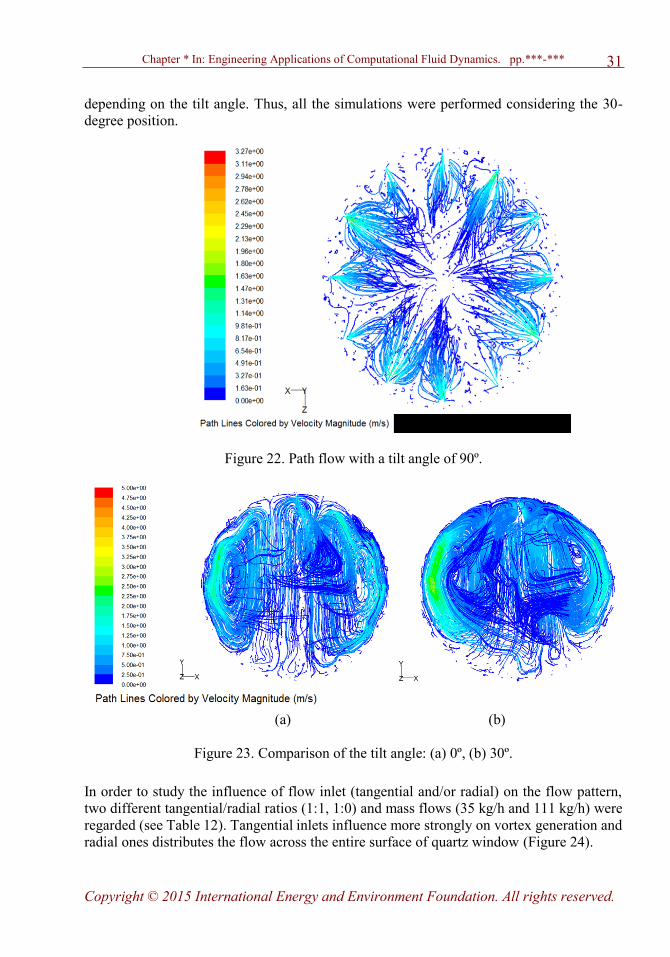
As previously mentioned, the path flow obtained for a 90-degree position does not show

vortex generation (see Figure 22). Furthermore, Figure 23 shows different flow patterns



31

depending on the tilt angle. Thus, all the simulations were performed considering the 30-

degree position.

Figure 22. Path flow with a tilt angle of 90º.

(a) (b)

Figure 23. Comparison of the tilt angle: (a) 0º, (b) 30º.

In order to study the influence of flow inlet (tangential and/or radial) on the flow pattern,

two different tangential/radial ratios (1:1, 1:0) and mass flows (35 kg/h and 111 kg/h) were

regarded (see Table 12). Tangential inlets influence more strongly on vortex generation and

radial ones distributes the flow across the entire surface of quartz window (Figure 24).



32

(a) (b)

(c) (d)

Figure 24. Influence of the type of flow inlet: (a) mass flow=35 kg/h, tangential/radial

ratio=1:1, (b) mass flow=35 kg/h, tangential/radial ratio=1:0, (c) mass flow=111 kg/h,

tangential/radial ratio=1:1, (d) mass flow=111 kg/h, tangential/radial ratio=1:0.

In order to determine the predominant type of flow inlet to favour the vortex generation, the

previous mass flows (35 kg/h and 111 kg/h) and several different tangential/radial ratios

(1:2, 2:1 and 3:1, see Table 12) were considered in the simulation, obtaining the following

flow distributions (Figure 25).



33

(a) (b)

(c) (d)

Figure 25. Evaluation of the predominant type of flow inlet: (a) mass flow=35 kg/h,

tangential/radial ratio=1:2, (b) mass flow=111 kg/h, tangential/radial ratio=1:2, (c) mass

flow=35 kg/h, tangential/radial ratio=2:1, (d) mass flow=111 kg/h, tangential/radial

ratio=2:1.

It is observed that the vortex actually appears when tangential inlet is predominant for both

mass flows. To further analyse this fact, the ratio 3:1 was simulated. Figure 26 shows the

flow patterns obtained, where a more defined vortex is depicted.

For the purpose of the optimisation of mass flow, the ratios 2:1 and 3:1 were simulated for

an additional mass flow (50 kg/h). The results of its flow distribution have been included in

Figure 27.



34

a) b)

Figure 26. Evaluation of the predominant type of flow inlet: (a) mass flow=35 kg/h,

tangential/radial ratio=3:1, (b) mass flow=111 kg/h, tangential/radial ratio=3:1.

(a) (b)

Figure 27. Optimisation of the mass flow: (a) mass flow=50 kg/h, tangential/radial

ratio=2:1, (b) mass flow=50 kg/h, tangential/radial ratio=3:1.

The comparison between the flow patterns obtained from the simulation of the mass flows

mentioned demonstrates that high flows improve the vortex definition (see Figure 26b) and

lead to flow lines with higher velocities which make easier collecting the reactive particles.

Thus, the selection of the most appropriate operating conditions to avoid the impact of

these particles on the quartz window has considered the criteria of the best vortex definition

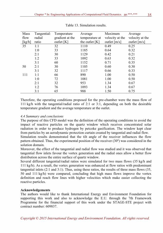
and the lowest temperature gradient at the outlet of the reactor pre-chamber. Table 13

summarise the results taken into account to define these conditions.



35

Table 13. Simulation results.

Mass

flow

[kg/h]

Tangential:

radial

ratio

Temperature

gradient at the

outlet [K]

Average

temperature at

the outlet [K]

Maximum

velocity at the

outlet [m/s]

Average

velocity at the

outlet [m/s]

35

50

111

1:1

1:0

2:1

1:2

3:1

2:1

3:1

1:1

1:0

2:1

1:2

3:1

32

33

30

33

60

30

32

66

72

32

76

65

1110

1185

1129

1092

1152

1105

1117

890

1081

953

1093

988

0.49

0.64

0.42

0.63

0.71

0.60

0.66

1.00

1.00

1.34

1.34

1.50

0.25

0.32

0.21

0.32

0.35

0.30

0.33

0.50

0.50

0.67

0.67

0.75

Therefore, the operating conditions proposed for the pre-chamber were the mass flow of

111 kg/h with the tangential/radial ratio of 2:1 or 3:1, depending on both the desirable

temperature gradient and the average temperature at the outlet.

4.4 Summary and conclusions

The purpose of this CFD model was the definition of the operating conditions to avoid the

impact of reactive particles on the quartz window which receives concentrated solar

radiation in order to produce hydrogen by petcoke gasification. The window kept clear

from particles by an aerodynamic protection curtain created by tangential and radial flow.

Simulation results demonstrated that the tilt angle of the receiver influences the flow

pattern obtained. Thus, the experimental position of the receiver (30º) was considered in the

solution domain.

Moreover, the effect of the tangential and radial flow was studied and it was observed that

tangential flow inlets favour the vortex generation and the radial ones allow a better flow

distribution across the entire surface of quartz window.

Several different tangential/radial ratios were simulated for two mass flows (35 kg/h and

111 kg/h). As a result, the vortex generation was enhanced at flow ratios with predominant

tangential inlets (2:1 and 3:1). Thus, using these ratios, the results of three mass flows (35,

50 and 111 kg/h) were compared, concluding that high mass flows improve the vortex

definition and reach flow lines with higher velocities which make easier collecting the

reactive particles.

Acknowledgements

The authors would like to thank International Energy and Environment Foundation for

supporting this work and also to acknowledge the E.U. through the 7th Framework

Programme for the financial support of this work under the STAGE-STE project with

contract number: 609837.



36

References

[1] Schlumberger Energy Institute. Leading the energy transition: Concentrating Solar

Power. SBC Energy Institute, 2013.

[2] United States Department of Energy. 2014: The year of concentrating solar power.

DOE, 2014.

[3] International Renewable Energy Agency (IRENA) and Energy Technology Systems

Analysis Programme (ETSAP). Concentrating Solar Power. Technology brief. IEA-

ETSAP and IRENA, 2013.

[4] AT Kearney and ESTELA. Solar Thermal Electricity 2025. A.T. Kearney,

www.atkearney.com, 2010.

[5] International Energy Agency (IEA). Concentrating Solar Power Technology

Roadmap, 2010a. IEA, www.iea.org, 2010.

[6] International Renewable Energy Agency (IRENA). Concentrating Solar Power-

Renewable Energy Technologies, Cost Analysis Series. IRENA working paper,

www.irena.org, 2012.

[7] KME Italy S.P.A. Cavo scaldante ad isolamento minerale. Data sheet of the

resistor, 2008.

[8] Fluent-Inc. Gambit 2.2 User’s Guide. Lebanon, NH, 2004.

[9] Batchelor G.K. An Introduction to Fluid Dynamics. Cambridge University

Press, 1967.

[10] Fluent-Inc. Fluent 6.2 User’s Guide. Lebanon, NH, 2005.

[11] Blazek J. Computational Fluid Dynamics: Principles and Applications.

Elsevier, 2005.

[12] Dantzig J.A., Tucker III C.L. Modeling in Materials Processing, Cambridge

University Press, 2001.

[13] Roldán M.I. Simulación y evaluación del receptor HiTRec II: estudio de la influencia

del viento y de la temperatura del aire de recirculación. PSA internal document:

USSC-SC-QA-79, 2013.

[14] León J., Clavero J., Valenzuela L., Zarza E., García G. PTTL – A life-real size test

loop for parabolic trough collectors. Energy Procedia 2014, 49, 136-144.

[15] Romero M., Téllez F.M., Valverde, A. Operación, Ensayo y re-Evaluación del

Receptor Volumétrico de Aire PHOEBUS-TSA. Campaña de Ensayos Abril 1999.

Project report (Ref. TSA_99-T01-IN-C01), 1999.

[16] Haeger M., Keller L., Monterreal R., Valverde A. Phoebus Technology program

Solar Air receiver (TSA): operational experiences with the experimental set-up of a

2.5 MWth volumetric air receiver (TSA) at the Plataforma Solar de Almería. Project

report (Ref. PSA-TR02/94), 1994.

[17] Ballestrín J., Monterreal R. Hybrid heat flux measurement system for solar central

receiver evaluation. Energy 2004, 29, 915-924.

[18] Becker M., Fend T., Hoffschmidt B., Pitz-Paal R., Reuter O., Stamatov V. et al.

Theoretical and numerical investigation of flow stability in porous materials applied

as volumetric receivers. Sol. Energy 2006, 80, 1241-1248.

[19] Roldán M.I., Smirnova O., Fend T., Casas J.L., Zarza E. Thermal analysis and

design of a volumetric solar absorber depending on the porosity. Renew. Energ.

2014, 62, 116-128.

http://www.atkearney.com/

http://www.iea.org/

http://www.irena.org/



37

[20] Fend T., Hoffschmidt B., Pitz-Paal R., Reutter O. Cellular ceramics use in solar

radiation conversion. Chapter in Cellular ceramics: structure, manufacturing and

applications (Ed. Scheffer M., Colombo P.), pp. 523-546, Weinheim: Willey-VCH

GmbH & Co. KgaA, 2005.

[21] Special Metals Corporation. Data sheet: Inconel® alloy 601. Publication number

SMC-028, 2005.

[22] ThyssenKrupp VDM. Data sheet: Nicrofer® alloy 800. Data sheet number 4029,

2002.

[23] Roldán M.I. Diseño y análisis térmico de un sistema receptor volumétrico para un

horno solar de alta temperatura. ISBN 978-84-7834-696-7. CIEMAT, 2013.

[24] Z'Graggen A., Haueter P, Maag G, Vidal A, Romero M, Steinfeld A. Hydrogen

production by steam gasification of petroleum coke using concentrated solar power-

III. Reactor experimentation with slurry feeding. Int. J. Hydrog. Energy 2007, 32,

992-996.

[25] Rodat S., Abanades S., Sans J.L., Flamant G. Hydrogen production from solar

thermal dissociation of natural gas: development of a 10 kW solar chemical reactor

prototype. Sol. Energy 2009, 83, 1599-1610.

[26] Roldán M.I., Zarza E., Casas J.L. Modelling and testing of a solar-receiver system

applied to high-temperature processes. Renew. Energ. 2015, 76, 608-618.

[27] Denk T, Valverde A., López A., Steinfeld A., Haueter P., Zacarías L. et al. Upscaling

of a 500 kW solar gasification plant for steam gasification of petroleum coke.

Proceedings of the SolarPACES conference. Berlin, 2009.

[28] Vargaftik N.B, Vinogradov Y.K., Yargan V.S. Handbook of physical properties of

liquids and gases. Begell House, 1989.

[29] Fleischmann Iberica. Data Sheet: Fisa-Lite 170. Data sheet number

I-023/Rev.02/11.10.00, 2000.

M.I. Roldán completed her Degree in Chemical Engineering (2005) at the University

of Granada (Spain) and a doctoral fellow was awarded to her in Solar Fuels and

Solarisation of Industrial Processes Group at Plataforma Solar de Almería (Spain) in

2008. She received her Master’s degree in Chemical Engineering (2009) and finished

her PhD in the Department of Chemical Engineering at the University of Almería

(2012). She has 7 years of experience as solar researcher, mainly in the field of

Computational Fluid Dynamics simulation applied to Concentrating Solar

Technologies. She has collaborated in the thermal analysis and optimisation of

different concentrating solar systems. As a result of her research, she has published

5 papers in peer-reviewed journals, 1 book chapter and 1 book. She has participated in

6 international scientific conferences, 5 research projects and 6 scientific/technical

reports. She has been member of one doctoral thesis tribunal and reviewer in 5 international scientific

journals and in several conferences. Dr. Roldán is currently collaborating with different research areas using

CFD simulation in the solar thermal field at the Plataforma Solar de Almería.

E-mail address: [email protected]



38

J. Fernández-Reche holds his Degree in Physics by the University of Granada (Spain)

in 1995. He has 15 years of experience as solar researcher, mainly in the field of point

focus technologies. Experience in design and simulation of central receivers systems;

definition, coordination, and supervision of testing procedures; operation and

evaluation of several solar central receiver technologies (water/steam, air, molten

salt...); geometrical qualification of solar concentrators (parabolic-troughs, heliostat

and parabolic dishes). He is coauthor of 10 papers in peer-reviewed journals, about 40

communications to international conferences and more than 100 scientific or technical

project reports. Mr. Fernández-Reche is member of the International Solar Energy

Society and also member of national and international standardization committees

related to Solar Thermal Electricity technology.


L. Valenzuela has a Ph.D. by the University of Almería (2007), a Degree in Physics

(1994) and a Degree in Electronics Engineering (1996) by University of Granada

(Spain). She has more than 17 years of experience in solar thermal concentrating

technologies. She works in design, modelling and simulation of line-focus solar

systems; definition, coordination, and supervision of testing procedures for solar

collectors; operation and process control of parabolic-trough collectors with thermal

oil, pressurized water or direct steam generation; and evaluation of solar components

and systems. She is co-author of 30 papers in peer-reviewed journals, 53

communications to international conferences, 2 books, 10 books chapters, and more

than 75 scientific and technical reports. Dr. Valenzuela is currently leading the

Medium Concentration group of the R+D Unit devoted to solar concentrating systems

of the Plataforma Solar de Almería (Spain). She belongs to the Spanish standardization committee AENOR

CTN 206 and the international IEC TC 117.


A. Vidal has a Degree in Chemistry. Head of Solar Hydrogen Group at CIEMAT

since September 2008 with R&D activities on solar thermal power, solar hydrogen,

thermochemical cycles, etc. Technical and scientific experience and know-how on

solar chemistry, solar detoxification, solar hydrogen and solar power acquired at

CIEMAT and Plataforma Solar de Almería (SPAIN) during the last 20 years.

Participation in more than 30 R&D projects in energy research, 15 of them financed

by the European Commission. Author of more than 20 research articles in journals

and books. Experience as member of Spanish and International scientific and

technical committees: Operating Agent for Task II (Solar Chemistry) at the

SolarPACES Implementing Agreement of the IEA, since April 2007. Peer reviewer

of scientific and technical magazines and publications.


E. Zarza has a Ph.D. by the University of Seville (2003), a Degree in Industrial

Engineering (1985) by University of Seville (Spain). He has 29 years of experience in

solar thermal concentrating technologies, thus coordinating and participating in many

national and international R+D projects related to parabolic trough collectors and their

applications (seawater desalination, direct steam generation and process heat

applications). He is co-author of 6 books, 35 papers in peer-reviewed journals, 14 book

chapters and 84 communications to international conferences, Dr. Zarza is currently

the Head of the R+D Unit of the Plataforma Solar de Almería (PSA, Spain) devoted to

solar concentrating systems, a multi-disciplinary team composed of 31 researchers

covering all the issues related to these solar systems and their applications. He is

member of the Scientific Committee of ESTELA (European Solar Thermal Electricity

Association), CIC-Energigune and KIC-Innoenergy


Date post:	26-Mar-2018
Category:	Documents
Upload:	vodieu
View:	216 times
Download:	3 times

INTERNATIONAL ENERGY AND ENVIRONMENT thermosolar field is still ... in this chapter are some...

Documents