Interpreting the Great Moderation: Changes in the...

Interpreting the Great Moderation:Changes in the Volatility of EconomicActivity at the Macro and Micro Levels

Steven J. Davis and James A. Kahn

Most advanced economies have experienced a striking decline in thevolatility of aggregate economic activity since the early 1980s. Volatilityreductions are evident for output and employment at the aggregate level

and across most industrial sectors and expenditure categories. Inflation and infla-tion volatility have also declined dramatically. Previous studies offer several poten-tial explanations for this “Great Moderation.” Some studies credit improved mon-etary policy for reductions in the volatility of real economic activity and inflation(for example, Clarida, Cali, and Gertler, 2000). Others suggest that financialinnovation and increased global integration play a role (Dynan, Elmendorf, andSichel, 2006). Still others, pointing to evidence that output volatility fell more thansales volatility, highlight the potential role of better inventory control methods (forexample, Kahn, McConnell, and Perez-Quiros, 2002). Another line of researchstresses “good luck” in the form of smaller exogenous shocks (for example, Stockand Watson, 2003).

These explanations are not mutually exclusive. As Bernanke (2004) remarks inhis discussion of the Great Moderation: “Explanations of complicated phenomenaare rarely clear cut and simple, and each . . . probably contains elements of truth.”The main elements can also interact in complicated ways. Perhaps, for example, the

y Steven J. Davis is William H. Abbott Professor of International Business and Econom-ics, Graduate School of Business, University of Chicago, Chicago, Illinois, and ResearchAssociate, National Bureau of Economic Research, Cambridge, Massachusetts. James A.Kahn is Visiting Professor of Finance, Wharton School, University of Pennsylvania,Philadelphia, Pennsylvania, and Visiting Scholar, Stern School of Business, New YorkUniversity, New York City, New York. Davis’s e-mail address is �[email protected]�.Kahn’s e-mail address is �[email protected]�.

Journal of Economic Perspectives—Volume 22, Number 4—Fall 2008—Pages 155–180

unsuccessful monetary policy of the 1970s, or the more successful policy thatfollowed, facilitated the spread of volatility-reducing financial innovations. Orperhaps sound monetary policy is easier when shocks are milder. Nonetheless, evenif no single factor fully explains the phenomenon, it is useful to amass evidence forand against particular hypotheses.

We seek to address two fundamental questions about the Great Moderation:What are its causes? And does it matter for economic welfare? We consider a varietyof evidence related to the Great Moderation, drawing mainly on U.S. data, andwork towards a story with a few key themes. Unlike most research on the topic, oursconsiders volatility behavior at the micro level for clues about the sources andconsequences of aggregate volatility changes. From a welfare perspective, a keyissue is whether the Great Moderation led to lower consumption volatility and lesseconomic uncertainty for individuals and households. It matters, for example,whether the Great Moderation mainly involves transient sources of income volatilityor long-lasting shocks, since consumers can more readily buffer transient incomemovements. It also matters whether the decline in aggregate volatility translatedinto a decline in volatility at the micro level.

As it turns out, the micro story is complex. The average volatility of firm-levelemployment growth fell after the mid-1980s (Davis, Haltiwanger, Jarmin, andMiranda, 2007). At the individual level, several indicators point to a large declinein the risk of unwanted job loss after the early 1980s (Davis, forthcoming). Declinesin firm-level volatility and job-loss risks fit naturally with the decline in aggregatevolatility. However, when we consider household-level consumption changes, wefind no evidence for a decline in volatility after 1980. The evidence on individualearnings uncertainty points to a longer-term rise, not a decline. Reconciling thefuller set of facts about micro volatility trends with the aggregate volatility declinepresents a significant challenge, which we meet only part way.

We begin with some facts about the Great Moderation, centered on thereduced volatility of real activity and the stabilization of inflation. Our interpreta-tion of this evidence casts doubt on explanations for the Great Moderation thatemphasize better monetary policy or financial innovation. Instead, it points towarda technological story focused on the durable goods sector, and in particular oninventory investment. We then examine inventory behavior in more detail andprovide additional evidence of improved supply-chain management and a specificstory for how it can explain reduced volatility. Next, we consider whether evidenceabout volatility in micro data is consistent with our story. We present evidence onvolatility in household-level consumption data and briefly discuss research onearnings and income uncertainty. In the end, we conclude that a substantialcomponent of the Great Moderation reflects reductions in short-term volatility thathave had little or no apparent impact on consumption risks at the household level.

We will not devote much space to the “good luck” hypothesis, even though anumber of influential studies find support for it. We interpret these findings asdemonstrating the need for better models to explain the volatility reductions orfor convincing evidence that measurable and plausibly exogenous, economic

156 Journal of Economic Perspectives

disturbances—oil supply disruptions, wars, or weather, for example—can explainobserved declines in the volatility of economic activity.1

There is also an older debate about whether economic volatility fell afterWorld War II in comparison to the prewar era. That discussion focused on mea-surement issues and data quality. Romer (1986) argued that the apparent postwarstabilization was only a “figment of the data” resulting from improved statisticalmethods and more complete measurement in the postwar era. Our discussion willfocus exclusively on postwar data where, subject to controlling for compositionalchanges, we believe the data permit meaningful comparisons over time.

Declines in the Volatility of Aggregate Economic Activity

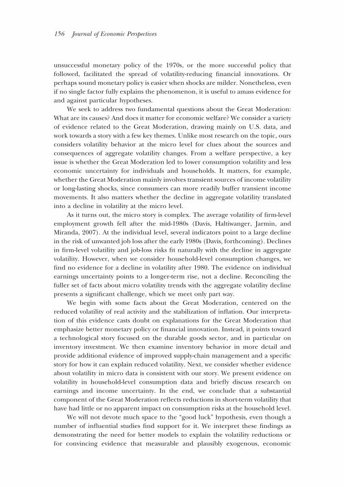
An abrupt drop in the volatility of U.S. real GDP growth in the early 1980s,shown in Figure 1, provided the initial impetus for research on the Great Moder-ation. Early findings of a discrete break in volatility around 1984 (Kim and Nelson,

1 For more discussion of the “good luck” hypothesis, see, for example, Stock and Watson (2003),Justiniano and Primiceri (2006), and Ahmed, Levine, and Wilson (2004). Along these lines, a recentstudy (Giannone, Lenza, and Reichlin, 2008) argues that the econometric models that underlie thesupport for good luck hypothesis are too simple. When they examine more complex models with alarger number of variables, they find that the reduced volatility comes from a change in the propagationof shocks rather than in the size of the shocks.

Figure 1GDP Growth, 1947–2007(quarterly, annual rate in percent)

-15

-10

-5

0

5

10

15

20

1950

1955

1960

1965

1970

1975

1980

1985

1990

1995

2000

2005

Source: National Income and Product Accounts.Note: Shaded periods represent NBER-designated recessions

Steven J. Davis and James A. Kahn 157

1999; McConnell and Perez-Quiros, 2000) encouraged a focus on comparisonsbefore and after 1984. This approach conceals the fact that many economic seriesdid not undergo an abrupt volatility drop around 1984. Some did so much earlier,some later, and for some, volatility trended down rather than dropped.

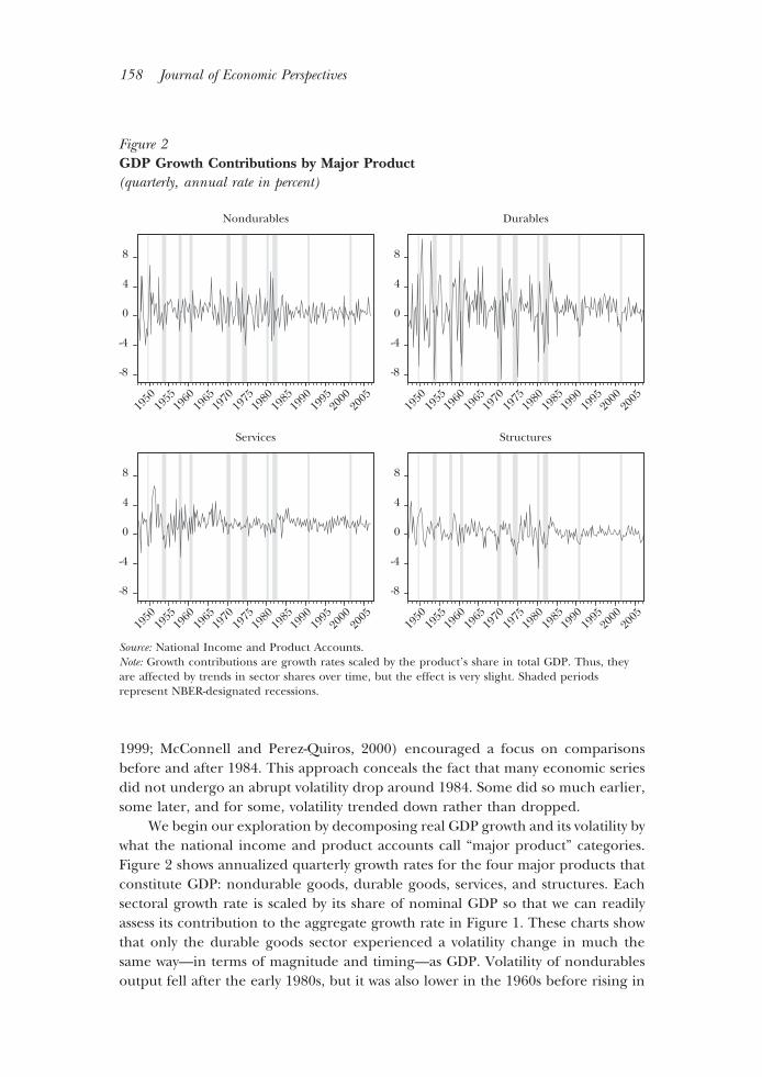
We begin our exploration by decomposing real GDP growth and its volatility bywhat the national income and product accounts call “major product” categories.Figure 2 shows annualized quarterly growth rates for the four major products thatconstitute GDP: nondurable goods, durable goods, services, and structures. Eachsectoral growth rate is scaled by its share of nominal GDP so that we can readilyassess its contribution to the aggregate growth rate in Figure 1. These charts showthat only the durable goods sector experienced a volatility change in much thesame way—in terms of magnitude and timing—as GDP. Volatility of nondurablesoutput fell after the early 1980s, but it was also lower in the 1960s before rising in

Figure 2GDP Growth Contributions by Major Product(quarterly, annual rate in percent)

-8

-4

0

4

8

1950

1955

1960

1965

1970

1975

1980

1985

1990

1995

2000

2005

Nondurables

-8

-4

0

4

8

Durables

-8

-4

0

4

8

Services

-8

-4

0

4

8

Structures

1950

1955

1960

1965

1970

1975

1980

1985

1990

1995

2000

2005

1950

1955

1960

1965

1970

1975

1980

1985

1990

1995

2000

2005

1950

1955

1960

1965

1970

1975

1980

1985

1990

1995

2000

2005

Source: National Income and Product Accounts.Note: Growth contributions are growth rates scaled by the product’s share in total GDP. Thus, theyare affected by trends in sector shares over time, but the effect is very slight. Shaded periodsrepresent NBER-designated recessions.


the 1970s, and it was never nearly as high as the volatility of durables. Thus, thevolatility decline for nondurables—such as it was—figures only modestly in thestabilization after the early 1980s. Likewise, the service sector was never nearly asvolatile as durable goods output; and moreover, its volatility fell in the early 1960sand again in the 1970s, long before the onset of the Great Moderation in the 1980s.Structures underwent a decline in output volatility similar in timing to that foroverall GDP, but the size of the sector and its contribution to GDP volatility aremodest. Thus, the drop in GDP volatility appears most closely related to develop-ments in the durable goods sector.

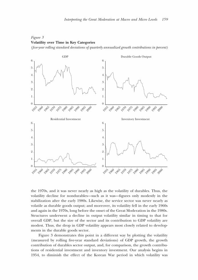
Figure 3 demonstrates this point in a different way by plotting the volatility(measured by rolling five-year standard deviations) of GDP growth, the growthcontribution of durables sector output, and, for comparison, the growth contribu-tions of residential investment and inventory investment. Our analysis begins in1954, to diminish the effect of the Korean War period in which volatility was

Figure 3Volatility over Time in Key Categories(five-year rolling standard deviations of quarterly annualized growth contributions in percent)

0

1

2

3

4

5

6

1955

1960

1965

1970

1975

1980

1985

1990

1995

2000

GDP

0

1

2

3

4

5

6Durable Goods Output

0

1

2

3

4

5

6Residential Investment

0

1

2

3

4

5

6Inventory Investment

1955

1960

1965

1970

1975

1980

1985

1990

1995

2000

1955

1960

1965

1970

1975

1980

1985

1990

1995

2000

1955

1960

1965

1970

1975

1980

1985

1990

1995

2000

Interpreting the Great Moderation at Macro and Micro Levels 159

unusually high even for that era. Inventory investment, which overlaps with durablegoods output, displays nearly as large a drop in volatility as durable goods output,despite having an average GDP share of less than 1 percent. Residential investmentexperienced a large drop in volatility beginning in the early 1980s, but its impact onoverall GDP volatility is limited by its small share of aggregate activity (about5 percent). Thus, the residential investment sector played a small role in the GreatModeration unless it had disproportionately large spillover effects on other sectors.Volatility declines in other components of GDP (not shown) are also relativelymodest and not necessarily synchronized with the Great Moderation (Kahn, 2008).

Figure 3 also suggests that both for total GDP and especially for durables, thevolatility decline in the early 1980s was an acceleration of a trend dating back toWorld War II. Indeed, Blanchard and Simon (2001) argue that the suddenness ofthe volatility drop is more apparent than real—that, in fact, large shocks in the1970s and a deep contraction in the early 1980s obscure the longer-term volatilitydecline that began well before the 1980s. The idea that the 1970s (really the periodfrom 1970 to 1983) were exceptional will be a recurring theme in our discussion. Butwhereas Blanchard and Simon stress that volatility declines occurred across a broadrange of GDP components, we argue that only the volatility decline in the durablegoods sector is comparable to that of overall GDP in trend, timing, and magnitude.

A related question is the extent to which the Great Moderation reflects asecular shift away from relatively volatile sectors. In particular, the rising GDP shareof a low-volatility sector like services might be expected to moderate outputvolatility. It turns out, however, that the secular shift toward services plays a modestrole in the reduction of overall output volatility. Specifically, using 1984:1 as a breakpoint, we calculate that the volatility of quarterly GDP fell by 1.97 percentage points(as measured by standard deviations of annualized growth rates). If we reconstructGDP growth by fixing output shares for the four major product categories at their1959 values, we instead calculate that the volatility of quarterly GDP growth fell by1.75 percentage points. According to this calculation, broad sectoral shifts accountfor about 12 percent of the long-term decline in GDP volatility.

What about shifts within major product categories? For example, are shiftsaway from automobiles and toward electronic equipment partly responsible for thelarge decline in durables volatility? Disaggregated output data from the nationalincome and product accounts are available only annually, which throws out higher-frequency volatility, and only back to 1977, which leaves only seven observationsprior to the commonly used break point of 1984. A useful alternative is to constructoutput data from the Bureau of Economic Analysis (BEA) series on constant-dollarshipments and inventories, available monthly on a consistent basis from 1967 to1997 for durable goods manufacturing and eleven industries at the two-digitStandard Industrial Classification (SIC) level. These data show a pattern of greatlyreduced volatility after 1983, and they confirm that volatility varies greatly across thedisaggregated industries. However, repeating the same type of exercise as before,we find that volatility in the durables sector fell slightly more on a fixed-weight basis(51 percent) than the 48 percent drop from 1967–83 to 1984–97 in the raw data.


We conclude that long-term sectoral shifts contribute to, but are not the main forcebehind, the Great Moderation.2

Another illuminating fact about the Great Moderation is that volatility fellsubstantially more, and earlier, for output than for final sales. In the durable goodssector, for example, comparing pre- and post-1983, the standard deviation ofoutput growth declined from 17.8 percent to 7.7 percent, whereas the standarddeviation of sales growth declined only from 10.3 to 8.4 percent (McConnell andPerez-Quiros, 2000; Blanchard and Simon, 2001; Kahn, McConnell, and Perez-Quiros, 2002). Since inventory investment makes up the difference between outputand final sales, this fact implies a change in inventory behavior—either a reductionin the volatility of inventory investment or a change in the covariance betweeninventory investment and sales. By national income accounting conventions, theservices and structures sectors do not carry inventories, so the source of the changein inventory behavior must by definition lie in the goods sector.3 We will return tothis topic below when we discuss inventory behavior in more detail.

Finally, not all volatility matters equally for economic welfare. Households cansave and borrow to buffer their consumption against income volatility, particularlyif the income movements are transitory. Thus the volatility of consumption expen-diture is much lower than that of GDP, especially if one removes expenditures ondurables (which are really a form of investment). In fact, whereas the volatility ofreal GDP growth fell by 2.5 percentage points post-1983, from 4.5 percent to2 percent, the volatility of real expenditures on nondurables and services fell by just0.8 percentage points, from 2.1 percent to 1.3 percent. This pattern suggests thatthe decline in GDP volatility may have had only a modest impact on welfare.

One possibility is that a substantial part of the output volatility decline has beenof the transitory type. To examine this, we consider how output volatility is appor-tioned across different “frequencies”—fluctuations of different durations. We canthink of fluctuations in economic activity as being composed of cycles of varyinglength: daily, weekly, yearly, or longer. The amplitude of fluctuations in activitybetween daytime and nighttime, or weekday to weekend, is considerably larger thanthat between business cycle peaks and troughs; yet these “high-frequency” fluctu-ations are usually seen as beneficial or benign. Even seasonal fluctuations areregarded as much less consequential for economic welfare in a modern economy,

2 Another way to cut the data is to decompose the production function into factor input and productivitycomponents. Stiroh (2005) decomposes output growth into the growth of hours worked and labor produc-tivity. He finds that the volatility of both components fell and that their covariance declined. Gali andGambetti (2007) provide additional evidence of a major shift in the pattern of comovements among output,hours, and labor productivity. They interpret the evidence as favoring a “structural change” interpretation ofthe Great Moderation (rather than lower shock volatilities) in the form of more aggressively anti-inflationarymonetary policy and reduced labor adjustment costs. In contrast, Arias, Hansen, and Ohanian (2007) arguethat a decline in the volatility of the Solow residual points toward the reduction of “productivity-like” shocksin the context of a real business cycle model of fluctuations.3 In structures, construction is counted as part of final output (see, for example, �http://www.census.gov/const/c30/definitions.pdf�). There is, however, evidence of a change in inventory behavior in residentialconstruction, even though it is not treated as such in the national income and product accounts (Kahn,2000).


partly because of their relatively short duration and partly because of their predict-able nature. Indeed, the predictable seasonal component is typically removed fromeconomic time series via “seasonal adjustment” so as to isolate the more conse-quential, unpredictable part.

Fluctuations of a few years or longer, including the so-called business cycle, canhave adverse welfare consequences because they are much less predictable andbecause they are longer and cannot be relied on to average out. At a practical level,consumers have greater difficulty using savings to buffer expenditures against theuncertainty related to business cycles as compared to seasonal cycles. MiltonFriedman’s (1957) “permanent income” theory of consumption recognizes thispoint explicitly, predicting that consumers smooth spending relative to short-termor “transitory” fluctuations in income but not relative to “permanent” changes, bywhich he meant changes of at least several years duration.

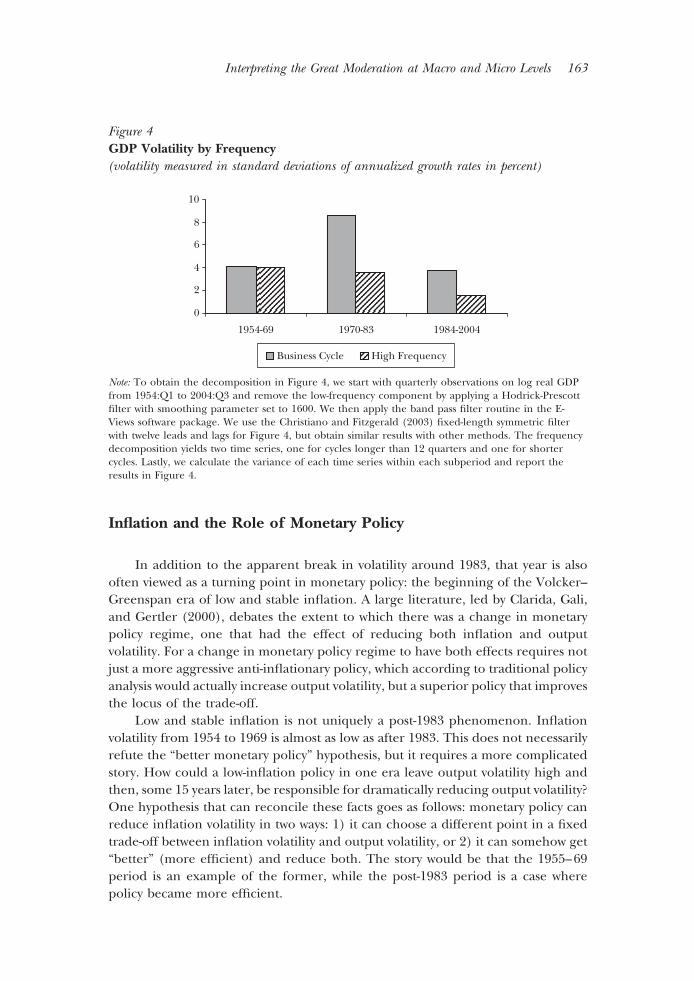
To understand the frequency dimension of the Great Moderation, it is helpful todivide the post-Korean War era into three periods: the relatively tranquil period from1954 to 1969, the turbulent period from 1970 to 1983, and the period from 1984 to thepresent. Figure 4 decomposes GDP volatility into a high-frequency component (cycleslasting fewer than 12 quarters) and a “business cycle” frequency component (longercycles) for each period. High-frequency volatility declined modestly from the first tothe second period, then fell sharply after 1983. This result suggests that the welfareconsequences of the Great Moderation might be modest, because much of the GreatModeration reflects a drop in the type of short-term volatility that presents fewerdifficulties for households in any event. Another piece of evidence pointing in thisdirection is the greatly diminished role of temporary layoffs in recessionary unemploy-ment movements since the mid-1980s (Groshen and Potter, 2003). At the householdlevel, consumption and living standards are probably less sensitive to temporary layoffsthan to permanent job loss. Temporary layoffs are also naturally associated with outputmovements of short duration, such as inventory corrections.

Figure 4 also shows that business cycle volatility jumped sharply in the middleperiod and then returned to approximately the same level as in the 1954–69period. Someone lumping the first two periods together might see a decline in bothtypes of volatility in the post-1983 era, but that approach masks highly volatilebusiness cycle fluctuations from 1970 to 1983 compared to before and after.4 Wehave repeated the exercise of Figure 4 for durable goods output and obtained asimilar pattern. This result reinforces the view that developments in the durablegoods sector play an important role in the Great Moderation.

4 Ahmed, Levin, and Wilson (2004), for example, provide evidence that the volatility decline after 1983was essentially uniform across all frequencies. Figure 4 does not contradict their finding, but it suggeststhat treating the 1970–83 period separately, especially with detrended levels rather than growth rates,could produce a different result. Kahn (2008) has more detailed results confirming the statisticalsignificance of the relative decline in high-frequency volatility.


Inflation and the Role of Monetary Policy

In addition to the apparent break in volatility around 1983, that year is alsooften viewed as a turning point in monetary policy: the beginning of the Volcker–Greenspan era of low and stable inflation. A large literature, led by Clarida, Gali,and Gertler (2000), debates the extent to which there was a change in monetarypolicy regime, one that had the effect of reducing both inflation and outputvolatility. For a change in monetary policy regime to have both effects requires notjust a more aggressive anti-inflationary policy, which according to traditional policyanalysis would actually increase output volatility, but a superior policy that improvesthe locus of the trade-off.

Low and stable inflation is not uniquely a post-1983 phenomenon. Inflationvolatility from 1954 to 1969 is almost as low as after 1983. This does not necessarilyrefute the “better monetary policy” hypothesis, but it requires a more complicatedstory. How could a low-inflation policy in one era leave output volatility high andthen, some 15 years later, be responsible for dramatically reducing output volatility?One hypothesis that can reconcile these facts goes as follows: monetary policy canreduce inflation volatility in two ways: 1) it can choose a different point in a fixedtrade-off between inflation volatility and output volatility, or 2) it can somehow get“better” (more efficient) and reduce both. The story would be that the 1955–69period is an example of the former, while the post-1983 period is a case wherepolicy became more efficient.

Figure 4GDP Volatility by Frequency(volatility measured in standard deviations of annualized growth rates in percent)

0

2

4

6

8

10

1954-69 1970-83

Business Cycle High Frequency

1984-2004

Note: To obtain the decomposition in Figure 4, we start with quarterly observations on log real GDPfrom 1954:Q1 to 2004:Q3 and remove the low-frequency component by applying a Hodrick-Prescottfilter with smoothing parameter set to 1600. We then apply the band pass filter routine in the E-Views software package. We use the Christiano and Fitzgerald (2003) fixed-length symmetric filterwith twelve leads and lags for Figure 4, but obtain similar results with other methods. The frequencydecomposition yields two time series, one for cycles longer than 12 quarters and one for shortercycles. Lastly, we calculate the variance of each time series within each subperiod and report theresults in Figure 4.


While one can tell such a story, little evidence supports it. Romer and Romer(2002a, 2002b) argue, in fact, that policy in the 1950s was similar to policy in the1990s. In addition, the “better monetary policy” story would have to account for therange of facts about the Great Moderation described in the previous section,including the long downward trend in durables output volatility, and the changesin inventory behavior implied by the small drop in sales volatility compared tooutput volatility.

A different argument for the “better monetary policy” hypothesis is that it isthe only story compatible with a discrete drop in volatility after the early 1980s.Improved inventory management is unlikely to have emerged suddenly. Andfinancial innovation, another proposed contributor to the Great Moderation, ismost plausibly a gradual process, even if there were specific discrete events such asthe demise of Regulation Q interest rate ceilings in the early 1980s (for example,Bernanke, 2007).

Monetary policy, on the other hand, can be subject to sudden changes in“regime.” In the last 20 years, for example, many central banks around the worldadopted “inflation targeting” regimes that arguably involve a discrete departure fromearlier policies. In October 1979, the Federal Reserve under Volcker shifted fromtargeting the federal funds rate to targeting nonborrowed reserves, a regime that lasteduntil 1983. A number of studies (for example, Clarida, Gali, and Gertler, 2000) provideevidence that the interest rate targeting regimes pre-1979 and post-1983 were funda-mentally different, the former resulting in both inflation and output instability.

Nonetheless, the evidence for an important shift in monetary policy regime isnot clear cut. Sims and Zha (2006) argue that changes in monetary policy regimeswere relatively inconsequential and in any case do not line up very well withchanges in volatility. In a series of papers, Orphanides (2002, for example) arguesthat the policy regime of the 1970s was not fundamentally different from earlierpolicies, but the Fed was hit with large structural changes (a higher “natural”unemployment rate and lower trend productivity growth) for which it had limitedand imperfect information in real time.

There are, moreover, good reasons to doubt the hypothesis that advances inthe conduct of monetary policy are responsible for the discrete drop in volatilitypost-1983. Modern research on monetary policy points to a variety of factors thatinfluence the efficacy of monetary policy. These include the credibility of thepolicymaker, transparency, and commitment to rules-oriented decision making.With hindsight, the Volcker–Greenspan era looks like a discrete break with theimmediate past, but it is not plausible that the Fed achieved enhanced credibilityovernight. In addition, increased transparency has been an evolutionary process.The Federal Open Market Committee began making public its interest rate targetdecisions only in 1994. It did not begin releasing statements explaining its policydecisions until 1998, and the informational content of these statements continuesto evolve. Thus, the contention that there was a discrete breakthrough for monetarypolicy in 1983 that explains the drop in output volatility after the early 1980s looksshakier under close scrutiny.

International evidence also provides grounds for skepticism about the role of


monetary policy. Since the early 1980s, most industrialized countries experiencedreduced output and inflation volatility, but with no clear connection to changes inmonetary policy. Some countries adopted the policy of “inflation targeting,” somedid not, and among those that did, there was considerable variety in its implemen-tation. Truman (2003) finds some evidence that inflation-targeting countries ex-perienced larger declines in output volatility, but there were differences in initialconditions between adopters and non-adopters. A more robust conclusion is thatvolatility dropped for nearly all industrialized countries, but the evidence is mixedregarding any connection with the timing and specifics of monetary policy changes.

The 1970s experience does point to a role for monetary policy in the GreatModeration, but not in the way usually emphasized by adherents of the “bettermonetary policy” explanation. The evidence described earlier points to an under-lying downward trend for aggregate volatility in much of the postwar era, inter-rupted by the turbulent 1970s (Blanchard and Simon, 2001). This reading of theevidence suggests that policy mistakes during the 1970s raised volatility for a time.Ending those mistakes with a return to policies resembling those of the 1950s andearly 1960s allowed volatility to return to its underlying postwar path. According tothis view, the resumption of sound monetary policy led to a large drop in volatilityby removing the role of policy mistakes in the 1970s, restoring an underlyingpostwar trend toward lower output volatility.

To summarize, the apparent suddenness of the drop in output volatility afterthe early 1980s does not persuade us that new-found skill in monetary policymakingdrove the Great Moderation. There is evidence that the Great Moderation beganbefore the Greenspan–Volcker era, and in any case monetary policy did notexperience a once-and-for-all change in 1983. The case is stronger that monetarypolicy mistakes or unusual shocks in the 1970s temporarily overwhelmed the forcesbehind the Great Moderation until the economic environment or policymakingreverted to something resembling earlier times. A persuasive case for a morepositive role for monetary policy requires: 1) a demonstration of how monetarypolicy in the post-1983 period is distinct from the policies of both the 1970s andearlier, and 2) a model that traces changes in sectoral volatility patterns andinventory behavior back to changes in monetary policy.

Inventory Behavior

The behavior of aggregate inventory investment has changed significantlysince the early 1980s. Here we focus on the durable goods sector, where the mostdramatic declines in output volatility occurred and where we have also seenevidence of a change in inventory behavior.5 Traditionally, the inventory literaturefocuses on disaggregated data, in particular on data for two-digit manufacturingindustries, but aggregate data have distinct advantages for our purposes. Disaggre-

5 We refer the reader to Bils and Kahn (2000), and the numerous references cited therein, fordiscussions of inventory behavior in the nondurable goods sector.


gated data are potentially misleading because it is impossible to judge whethermeasured changes in inventory behavior reflect genuine shifts or simply result fromless meaningful relocation of inventories between sectors. For example, if manu-facturers shift final goods inventories downstream to wholesalers and retailers, ormaterials inventories upstream to their suppliers, manufacturing inventories de-cline relative to their shipments. Yet that decline would be largely offset by inven-tory increases elsewhere in the economy, and a mere re-labeling would be misin-terpreted as evidence of structural change. We should note that the aggregate U.S.data we use are not entirely immune from this criticism—for example, firms couldshift materials inventories offshore to foreign suppliers.

Because output is the sum of final sales and inventory investment, we candecompose the variance of output growth rates into components for sales growthand inventory investment, plus a covariance term.6 The covariance term reflects theextent to which changes in inventory investment are positively correlated with salesgrowth and thereby add to output volatility. This decomposition allows us to trackthe contributions of sales and inventory investment to output volatility over time.Since sales volatility declines little, as mentioned above, we focus on the other twoterms of the decomposition. They are shown in Figure 5, which plots the rollingfive-year variance of the inventory investment term and the sales–inventory covari-ance term for the durable goods sector. Both terms show substantial downwardtrends, with the covariance term accounting for a very big drop in output volatilityafter the early 1980s. The results displayed in Figure 5 motivate additional investi-gation of inventory behavior.

We inspected the inventory–sales ratio for the durable goods sector using adata source that captures all durable goods inventories, including those situatedoutside the manufacturing sector. After peaking in the years 1982–83, the ratiotrends downward for nearly two decades (the solid line in Figure 6). By itself, thedownward trend in the inventory–sales ratio after the early 1980s is not proof oftechnical progress in inventory management. It could, instead, reflect composi-tional shifts or movement along a fixed technological trade-off in response to risinginventory carrying costs. Maccini, Moore, and Schaller (2004) argue that inventoryinvestment is responsive to very persistent changes in real interest rates. But thetiming of the break in the trend is striking. The inventory–sales ratio has alsobecome less volatile since the early 1980s, suggesting that businesses were hit by

6 Although inventory investment, because it can be negative, does not have a conventionally definedgrowth contribution, we can define it indirectly as the difference between the growth rate of output andthe growth contribution of final sales (Kahn, McConnell, and Perez-Quiros, 2002). Following Whelan(2002), we approximate the latter in terms of the real growth rate of sales and the nominal share of salesin output. Letting �xy denote the growth contribution of x to output y, where x � s for sales and x � ifor inventories, define the growth contribution of inventory investment as

�iy � �yy � �sy

where �sy � �ss�sy, �sy is the nominal share of s in y (measured as the average of current and laggedshares). The growth contribution of a variable to itself is just its growth rate.


Figure 5Contributions to Durables Output Variability(five-year rolling variances of growth contributions in percent)

-8

-4

0

4

8

12

1955

1960

1965

1970

1975

1980

1985

1990

1995

2000

Inventory investment Covariance

Figure 6Inventory-Sales Ratios in Durable Goods in Relation to Lead Times for MaterialsOrders in Manufacturing

40

60

80

100

120

.4

.5

.6

.7

1955

1960

1965

1970

1975

1980

1985

1990

1995

2000

Avg. lead time for orders* (in days, left scale)

Inventory-sales ratio,durable goods sector**(nominal, right scale)

Pre-1984 average = 65.8

Post-1984 average = 48.0

Day

s

*Source: Institute for Supply Management.**Source: Bureau of Economic Analysis.


smaller shocks, made smaller mistakes, or could more readily correct inventoryimbalances. Again, this pattern is not conclusive, but it is consistent with the ideaof improved inventory management technologies.

Kahn, McConnell, and Perez-Quiros (2002) describe results from forecastingequations with sales and inventories that point to another important differencebefore and after 1983. Before 1983, sales helped to forecast inventories more thaninventories helped to forecast sales. After 1983, they were similar, reflecting both adecrease in the usefulness of sales in forecasting inventories and an increase in theusefulness of inventories in forecasting sales. Moreover, the variance of salesforecast errors dropped precipitously, meaning that less of the variation in sales wasunpredicted given prior sales and inventories. These results are also consistent withthe idea that firms became better able to anticipate sales and adjust inventories inadvance.7

A Theory of Improved Inventory Control

One approach to assessing the role of improved inventory control is to beagnostic about the deeper story for technological change and look instead forchanges in parameters or shocks in a dynamic empirical model of inventorybehavior. McCarthy and Zakrajsek (2007) apply this approach to industry-levelmanufacturing data, which means their study is not directly comparable to ours aswe use GDP-level and sector-level data.8 They investigate the extent to whichchanges in the behavior of manufacturing inventories after 1983 reflect betterinventory management versus changes in what they call the “macro structure,”which includes shock magnitudes and the effects of monetary policy. They findevidence for both types of changes.

A second approach is to apply a specific optimizing model of improvedinventory control as in Kahn, McConnell, and Perez-Quiros (2002), which draws onearlier work by Kahn (1987) and Bils and Kahn (2000). In this model, firms carryfinished goods inventories to avoid stockouts (running out of inventory) in the faceof uncertain demand, trading off the cost of forgone profits against the cost ofcarrying inventories. If demand is serially correlated, mistakes in forecasting salesget magnified in production volatility so that production volatility exceeds the

7 Stock and Watson (2003) are skeptical of the role of inventory management in the Great Moderation.But they focus on four-quarter growth rates of economic time series, a transformation that essentiallyfilters out the higher-frequency volatility associated with inventory investment. Indeed, it should be nosurprise that inventory behavior appears less important in explaining the (smaller) volatility declines offour-quarter growth rates. Still, looking at four-quarter growth rates might be a reasonable thing to doif changes in high-frequency volatility were economically uninteresting or played a small role in theGreat Moderation, but we have argued otherwise. Stock and Watson’s other grounds for skepticism—thefact that sales volatility declined and that most inventories in manufacturing are raw materials or workin progress—are addressed in the next section.8 The disaggregated manufacturing data are subject to the measurement concerns raised earlier—boththe concerns about interactions with upstream and downstream activity, and also those about basingconclusions regarding the pre-1984 era on data that are primarily from the exceptionally volatile 1970s.


volatility of sales. To see why, suppose sales are unexpectedly low. Not only does thisleave the firm with more inventories than planned, but the firm now needs lowerinventories than it previously thought, because the persistence of the sales shockmeans lower sales than earlier forecasts for some time. Consequently, the firm cutsproduction by more than the current sales shock.9

Given this “stockout-avoidance” mechanism, suppose that better technologygives firms better information about future demand disturbances. Then firms makesmaller errors in production decisions, and the output volatility induced by cor-recting those errors diminishes. In addition, firms hold fewer inventories becausethey now face less uncertainty.

This story can account for reduced production volatility in absolute terms andrelative to sales volatility, but it has important drawbacks as a full explanation forthe changes in inventory, output, and sales behavior that we have documented.First, depending on when the firm receives information regarding demand shocks,the story has counterfactual implications for sales volatility. To see this point,suppose that better technology yields earlier information about a future demandincrease, in time to build up inventories before the demand increase arrives. Thenwhen the demand increase actually occurs, the firm draws down the inventories itbuilt up in anticipation. This result is consistent with the more negative correlationof inventory investment and sales, but the advance information has the counter-factual implication of greater sales volatility. Why? Because the firm is better able toaccommodate fluctuating demand by adjusting production without running out ofstock. Second, the stockout-avoidance approach does not apply so obviously ordirectly to the durable goods sector, much of which is best characterized asproduction-to-order rather than production-to-stock. A related point (see Blinderand Maccini, 1991, Humphries, Maccini, and Schuh, 2001, among others) is thatmost inventories, particularly in durable goods, are of materials or works in process,not final goods. Finally, while there is much anecdotal evidence concerning tech-nology improvements that provide better information about future sales, there isno direct evidence to assist in specifying a model.

Kahn (2008) develops a variation on the “better information” story thataddresses these concerns. Firms are production-to-order, and therefore hold onlyinventories of materials and works in process. They must order materials in ad-vance. A stockout occurs when works-in-process inventories are insufficient to allowthe firm to meet its (stochastic) orders, in which case the order gets added to thestock of unfilled orders. This setup is broadly consistent with the argument of Irvineand Schuh (2005), who attribute a substantial volatility decline to reducedco-movement between the manufacturing and trade sectors.

The intuition for how the model works is similar to that of the stockout-avoidance motive in Kahn (1987), described above, except that stockouts occur

9 Ramey and Vine (2006) argue that a reduction in the persistence of sales shocks in the automobileindustry was responsible, through a similar mechanism, for reducing the volatility of automobileproduction. Absent a deeper explanation for the reduced persistence, this explanation falls into the“good luck” category of explanations for the Great Moderation.


internally when the firm runs out of works-in-process inventories, rather thanexternally with finished goods stocks. Once again, because orders for final goodsare serially correlated, errors in forecasting demand get magnified in the volatilityof production (sales plus inventory investment). The key difference is that the firmproduces “to order” so that the improved information is not translated so directlyinto the accommodation of demand shocks and greater sales volatility. Sales areshipments of completed production, so some of the reduced production volatilitylessens the volatility of shipments, potentially offsetting the volatility-increasingeffect on sales (still present here) from improved accommodation of demandshocks.

So this model immediately addresses all but one of the objections raised above:It is specifically tailored to characteristics of the durable goods sector in that itassumes production-to-order rather than production-to-stock. It features works-in-process rather than final goods inventories. It has the property that better infor-mation about final orders has the potential to reduce the volatility of output andsales, the former more than the latter.

The remaining objection to this approach concerns the lack of direct evidenceof firms’ improved ability to forecast orders. Here we consider survey data obtainedfrom the Institute of Supply Management on average lead times for orders ofproduction materials. This is imperfect evidence and is not confined to the durablegoods sector, but it is striking nonetheless. The series is depicted in Figure 6,plotted against the inventory–sales ratio for the durable goods sector. While theaverage lead-time series does not exhibit the underlying downward trend of thevolatility series, it does feature a clear drop in level post-1983 relative to earlier. Italso shows some elevation in the more volatile 1970s.

What is the connection between shorter lead times and better information? Indeciding on its materials orders, the firm must base its forecast of future final goodsorders on whatever information it has available to it at the time. The longer the firmcan delay materials orders, the more information it has about its final goods ordersat any given date. Consequently, the firm can order materials more accurately andcarry smaller precautionary stocks.

Of course, what allows for shorter lead times is not modeled, but shorter leadtimes are taken as direct evidence of technical progress. Given that the goal of the“just-in-time” approach is greater flexibility to reduce the need to carry large stocks,this is a reasonable interpretation, but it may be only part of the story. For example,some of the increased lead times in the 1970s could be caused by Nixon-era pricecontrols, which created shortages and bottlenecks in materials deliveries. It wouldbe natural for firms concerned about an inability to obtain materials in a given timeframe to order farther in advance. This observation does not negate the mechanismin the model, but it points out that something other than technical progress canyield sustained movements in average lead times. Perhaps price controls, or eventhe high inflation of the 1970s, disrupted market signals and caused some of therise in lead times and volatility, but this hypothesis awaits further research.

There is little doubt that vast resources have been devoted to improving whatis generally referred to as “supply-chain management.” How this translates into


observable behavior and data is another question entirely. As Mentzer et al. (2001)write:

Despite the popularity of the term Supply Chain Management, both inacademia and practice, there remains considerable confusion as to its mean-ing. Some authors define SCM in operational terms involving the flow ofmaterials and products, some view it as a management philosophy, and someview it in terms of a management process.

They go on to define the term as “the systemic, strategic coordination of thetraditional business functions and the tactics across these business functions withina particular company and across businesses within the supply chain, for the pur-poses of improving the long-term performance of the individual companies and thesupply chain as a whole.” This definition is vague, but it clearly encompasses anumber of specifics, notably what the authors refer to as a logistics system: “the totalflow of materials, from the acquisition of raw materials to delivery of finishedproducts, to the ultimate users, as well as the related counter-flows of informationthat both control and record material movement.”

The strong prediction of the model is that shorter lead times give rise to areduction in output volatility and a somewhat smaller reduction in the volatility offinal sales. While the magnitudes of these declines depend on specifics such as theaverage inventory–sales ratio (which is endogenous in the model and depends onprice–cost markups and inventory holding costs) and the ratios of inputs to grossoutput at each stage of production, the qualitative results require only some degreeof persistence in final goods orders.

Changes in Volatility at the Micro Level

Thus far, our discussion suggests that much of the Great Moderation involvesa reduction in the volatility of durable goods output, and much of that reflectssignificant changes in inventory dynamics. We turn now to volatility trends at thelevel of firms, individuals, and households and ask whether the micro evidencesheds additional light on the Great Moderation and its consequences.

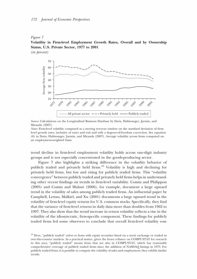
Firm-Level VolatilityFigure 7 plots the average volatility of firm-level employment in the United

States from 1977 to 2001. Davis, Hatiwanger, Jarmin, and Miranda (2007) constructthe figure using annual Census Bureau data on domestic employment for all firmsin the U.S. private sector. They calculate the rolling standard deviation of employ-ment growth rates for each firm and then compute the employment-weightedmean across firms for each year. As shown in the figure, the average volatility offirm-level employment fell from 49 percent in 1978 and 53 percent in 1987 to38 percent in 2001. Thus, firm-level volatility shows a substantial long-term decline,but the timing differs somewhat from the decline in aggregate output volatility. The


trend decline in firm-level employment volatility holds across one-digit industrygroups and is not especially concentrated in the goods-producing sector.

Figure 7 also highlights a striking difference in the volatility behavior ofpublicly traded and privately held firms.10 Volatility is high and declining forprivately held firms, but low and rising for publicly traded firms. This “volatilityconvergence” between publicly traded and privately held firms helps in understand-ing other recent findings on trends in firm-level variability. Comin and Philippon(2005) and Comin and Mulani (2006), for example, document a large upwardtrend in the volatility of sales among publicly traded firms. An influential paper byCampbell, Lettau, Malkiel, and Xu (2001) documents a large upward trend in thevolatility of firm-level equity returns for U.S. common stocks. Specifically, they findthat the variance of firm-level returns in daily data more than doubles from 1962 to1997. They also show that the trend increase in return volatility reflects a rise in thevolatility of the idiosyncratic, firm-specific component. These findings for publiclytraded firms led some observers to conclude that overall firm-level volatility rose

10 Here, “publicly traded” refers to firms with equity securities listed on a stock exchange or traded inover-the-counter markets. As a practical matter, given the heavy reliance on COMPUSTAT for researchin this area, “publicly traded” means firms that are also in COMPUSTAT, which has reasonablycomprehensive coverage of publicly traded firms since the addition of NASDAQ listings in 1973. Forpublicly traded firms, it is possible to compute the volatility of sales and employment; they exhibit similartrends.

Figure 7Volatility in Firm-level Employment Growth Rates, Overall and by OwnershipStatus, U.S. Private Sector, 1977 to 2001(in percent)

10

20

30

40

50

60

70

Ave

rage

firm

vol

atili

ty

All private sector Privately held Publicly traded

1977

1979

1981

1983

1985

1987

1989

1991

1993

1995

1997

1999

2001

Source: Calculations on the Longitudinal Business Database by Davis, Haltiwanger, Jarmin, andMiranda (2007).Notes: Firm-level volatility computed as a moving ten-year window on the standard deviation of firm-level growth rates, inclusive of entry and exit and with a degrees-of-freedom correction. See equation(6) in Davis, Haltiwanger, Jarmin, and Miranda (2007). Average volatility across firms computed onan employment-weighted basis.


sharply in recent decades, in puzzling contrast to the large drop in aggregatevolatility. Figure 7, however, shows otherwise.

Why does the volatility trend among publicly traded firms depart so sharplyfrom the overall trend? At one level, the answer is simple: publicly traded firmsaccount for less than one-third of private-sector employment, so there is muchroom for the trend among publicly traded firms to depart from the overall trend.Digging deeper reveals another, more interesting answer: there was a pronouncedshift in the economic selection process governing entry into the set of publiclytraded firms, and this shift greatly affected volatility trends among publicly tradedfirms.

To see this point, it is important to first recognize the large influx of newlylisted firms in the 1980s and 1990s. Fama and French (2004) report that thenumber of new listings (mostly initial public offerings) on major U.S. stock marketsjumped from 156 per year in the 1973–1979 period to 549 per year in 1980–2001.Remarkably, about 10 percent of listed firms are new in each year from 1980 to2001. Similarly, Davis, Haltiwanger, Jarmin, and Miranda (2007) report that firmsnewly listed in the 1980s and 1990s account for about 40 percent of employmentamong all publicly traded firms by the late 1990s. So the influx of new listings in the1980s and 1990s is large in number and rather quickly accounts for a large share ofactivity.

In addition, Fama and French (2004) provide evidence that new listings areriskier than seasoned public firms by a variety of measures and that they becomeincreasingly risky relative to seasoned firms after 1979. Based on their review ofthe evidence, they conclude that the upsurge of new listings explains much ofthe trend increase in idiosyncratic stock return volatility documented by Camp-bell, Lettau, Malkiel, and Xu (2001). They also suggest that there was a declinein the cost of equity that allowed weaker firms and those with more distantpayoffs to issue public equity. A more recent study by Brown and Kapadia (2007)reaches an even stronger conclusion. Using a regression methodology, theyfind that “there is generally no significant trend in idiosyncratic risk afteraccounting for the year a firm lists.” They also provide other evidence thatfirm-specific risks in the economy as a whole did not increase, even though thevolatility of firm-level equity returns rose because of an influx of successivelyriskier cohorts.

Davis, Haltiwanger, Jarmin, and Miranda (2007) obtain similar results forfirm-level employment volatility. Using a regression framework, they find thatsimple cohort effects for the year of first listing account for two-thirds of thevolatility rise among publicly traded firms from 1978 to 2001. In contrast, firm size,age, and industry effects—separately and in combination—account for little of thevolatility rise among publicly traded firms.

The Risk of Job LossAs discussed in Davis (forthcoming), a wide variety of labor market indicators

point to a secular decline in the risk of job loss. These indicators include unem-ployment inflows by experienced workers in the Current Population Survey (CPS);


the three-year job-loss rate in the CPS Displaced Worker Survey; several measuresfor the gross rate of job destruction at the level of individual employers; the numberof workers involved in mass layoff events; and the number of new claims forunemployment insurance benefits. All of these indicators point to a secular declinein the risk of job loss, although the extent and timing of the decline differ amongthe indicators. One of the most striking declines occurs in weekly new claims forunemployment insurance benefits. This measure of unwanted job loss fell from0.46 percent of nonfarm employment per week in 1970–1983 to 0.30 percent in1984–2007 and 0.27 percent since 1993.

Similarly, Current Population Survey data show a dramatic decline in unem-ployment inflows as a percentage of employment since the early 1980s. Davis,Faberman, Haltiwanger, Jarmin, and Miranda (2007) provide evidence that abouthalf of the long-term decline in unemployment inflow rates is explained by thereduction in the gross job destruction rates and the volatility of firm-level growthrates. Hence, their study provides evidence of a direct link between the seculardecline in firm-level volatility in Figure 7 and the secular decline in the incidenceof job loss.

Consumption Volatility and Income UncertaintyIn a permanent income model of consumption expenditures with stable

preferences, a decline in the variability of persistent income innovations producesa decline in the average magnitude of consumption changes. The intuition isstraightforward: smaller shocks to permanent income necessitate smaller adjust-ments to consumption. In the light of this implication, we investigate whether theaverage magnitude of household-level consumption changes rose or fell over time.A rise indicates an increase in economic uncertainty for the average household.Conversely, if the Great Moderation, the decline in firm-level volatility, and thereduced risk of job loss led to a more tranquil economic environment for theaverage household, then permanent-income logic implies a decline in the averagemagnitude of household-level consumption adjustments.

We take a simple approach to this issue using quarterly data from the interviewsegment of the Consumer Expenditure Survey, which has a short panel component.To measure the magnitude of household-level consumption adjustments, we com-pute the absolute value of the log change in consumption expenditures for eachhousehold and then average over households. This average value for the magni-tude of household-level consumption changes is our measure of consumptionvolatility. To assess whether trends in consumption volatility differ between richerand poorer households, we sort households into deciles of predicted consumptionbefore computing the consumption volatility.11 We sort the data this way to ensure

11 We restrict attention to nondurable goods and services and consider six-month changes in expendi-tures per adult equivalent in the consumer unit. Results are similar for three-month and nine-monthchanges. Our measure of adult equivalents is 1.0 times the first adult plus 0.7 times each additional adultin the same consumer unit plus 0.5 times each child in the consumer unit. We computed predictedconsumption based on a regression of log expenditures per adult equivalent on sex of the household


that we do not overlook important changes in consumption volatility for certaingroups, such as the lowest deciles, that we might miss by looking only at the overallaverage consumption volatility.

Figure 8 shows consumption volatility by decile of predicted consumption fortwo periods. There are two results. First, consumption volatility rises with theconsumption level in a given time period except at the low end of the distribution.Second, and more important for our purposes, there is no evidence for a declinein consumption volatility after the 1980s. In fact, Figure 8 points to a modestincrease in household consumption volatility over most of the consumption distri-bution. This second result is quite surprising given the declines in aggregate andfirm-level volatility and the reduced risk of job loss. Indeed, by capturing therecessions of the early 1980s and 1990s in the first of the two periods shown inFigure 8, one might worry that we stack the deck in favor of finding a trend declinein consumption volatility. For this reason, the absence of such a trend is all themore surprising. Taken at face value, and seen through the lens of the permanent-income theory, the second result says that the Great Moderation failed to deliver

head; a quartic polynomial in the head’s age; four educational attainment categories; marital status ofthe head; interview month; and employment status of the head and the head’s spouse, if there is one.We perform this sort based on the first interview with consumption expenditures for the consumer unit.

Figure 8Household-level Consumption Volatility by Deciles of Predicted Consumption

Abs

olut

e lo

g ch

ange

0.47

0.45

0.43

0.41

0.39

0.37

0.351 2 3 4 5 6 7 8 9 10

Absolute log ch

ange

0.47

0.45

0.43

0.41

0.39

0.37

0.35

Consumption decile

1980–1991

1992–2004

Note: We compute the absolute value of six-month log changes in expenditures on nondurable goodsand services per adult equivalent in each household. Averaging the absolute changes by time periodand decile yields the reported measure of consumption volatility.


more economic tranquility in the form of less consumption risk for the averagehousehold.

Given the surprising nature of the result in Figure 8, it would be reassuring toknow that other consumption data tell a similar story. Gorbachev (2007) uses dataon food expenditures in the Panel Study of Income Dynamics to estimate thevolatility of household consumption after controlling for predictable variationassociated with movements in real interest rates and changes in family structure.She finds that the volatility of household consumption expenditures increased overthe period from 1970 to 2002. Thus, data from both the Consumer ExpendituresSurvey and the Panel Study of Income Dynamics point to a trend rise in consump-tion volatility.

Another approach to assessing trends in economic uncertainty at the level ofhouseholds and individuals is to exploit income or earnings data. There is anenormous literature on earnings inequality and changes in the structure of wages,but few previous studies seek to quantify long-term changes in earnings uncertaintyfrom the vantage point of the individual. An exception is Cunha and Heckman(2007), who estimate the contribution of earnings uncertainty to the rise inearnings inequality. Their method uses data on schooling choices in combinationwith data on earnings outcomes to decompose the realized variance of earningsinto a component that is predictable by individuals and an unpredictable compo-nent that is not. They estimate a substantial rise in the variance of the unfore-castable component in the present value of earnings uncertainty among youngworkers. This result is broadly consistent with the evidence of increased consump-tion volatility.

A recent paper by Dynan, Elmendorf, and Sichel (2008) investigates thevolatility of household income using data from the Panel Study on Income Dynam-ics for households whose heads are at least 25 years old and not yet retired. Theyfind that the standard deviation of two-year percent changes in household-levelincome rose by a third from the early 1970s to the early 2000s, with trend increasesin all major age and education groups. They trace the rise of household incomevolatility to a greater frequency of very large income changes. While greater incomevolatility does not imply greater income uncertainty, it is certainly suggestive of sucha development. In this respect, the results in Dynan, Elmendorf, and Sichel lendcredence to the evidence of rising consumption volatility. In addition, Dynan,Elmendorf, and Sichel summarize many studies that investigate trends in earningsand income volatility or trends in estimated earnings uncertainty based on statis-tical models. Although the studies differ greatly in their particulars, none show adecline in income volatility or earnings uncertainty that even approximates thedecline in aggregate volatility, and the vast majority of the studies point to greatervolatility or uncertainty.

Summary of Micro Volatility Evidence and ImplicationsThe volatility of firm-level employment growth rates fell after the early to mid

1980s. The decline in average firm-level volatility is similar in magnitude to the


decline in aggregate volatility, but the timing differs. Although we did not discussit here, the volatility of state-level employment growth rates also fell after the 1980s(Carlino, DeFina, and Sill, 2007). Among publicly traded firms, the volatility in realactivity and in equity returns rose sharply after the early 1980s. This rise in volatilityamong publicly traded firms is a striking phenomenon, but it mainly or entirelyreflects shifts in the selection process governing which firms become public. Hence,considerable care is required when drawing inferences about the sources andnature of the Great Moderation from data on equity returns or from any datalimited to publicly traded firms.

Declines in firm-level volatility and gross job-destruction rates are closelylinked to declines in the risk of unwanted job loss, as reflected in sharply lowerunemployment inflows after the early 1980s. In this respect, data on aggregatevolatility, average firm-level volatility, job destruction rates, and the incidence ofunemployment all point to a much more quiescent economic environment sincethe early 1980s. In contrast, data on labor earnings, income, and consumptionexpenditures do not conform to a story of greater tranquility and lower uncertaintyat the household or individual level. Although there is much room for furtherresearch, the available evidence suggests at least a modest increase in individualand household economic uncertainty. Assuming that this assessment of trends inhousehold-level consumption volatility and related measures of individual uncer-tainty holds up under further study, it highlights a puzzle that research on the GreatModeration has yet to confront: why has the dramatic decline in the volatility ofaggregate real activity and the roughly coincident decline in firm-level volatility andjob-loss rates not translated into sizable reductions in earnings uncertainty andconsumption volatility facing individuals and households?

We do not know the answer to this question, but we conjecture that greaterflexibility in pay setting for workers played a role, possibly a major one. Greater payflexibility is consistent with the rise in wage and earnings inequality in U.S. labormarkets since 1980 and with increases in individual income volatility and earningsuncertainty. If these developments involve a rise in the variance of idiosyncraticpermanent income shocks to households, then household consumption volatilityalso rises according to permanent income theory. Greater wage (and hours)flexibility also leads to smaller firm-level employment responses to idiosyncraticshocks and smaller aggregate responses to common shocks, because firms canrespond by adjusting compensation rather than relying entirely on layoffs andhires. By the same logic, wage adjustments can substitute for unwanted job loss. So,at least in principle, greater wage flexibility offers a unified explanation for the risein wage and earnings inequality, flat or rising volatility in household consumption,a decline in job-loss rates, and declines in firm-level and aggregate volatility mea-sures. Sources of greater pay flexibility include the decline of real minimum wages,a diminished role for private sector unionism and collective bargaining, intensifiedcompetitive pressures that undermined rigid compensation structures, the growthof employee leasing and temp workers, and the erosion of norms that formerlyrestrained wage differentials and prevented wage cuts.


Concluding Remarks

We summarize the main elements of our evidence and analysis. First, macro-economic volatility has generally trended downward in the postwar United States(and in many other countries as well), interrupted by heightened turbulence in the1970s and early 1980s. Otherwise, however, much of the Great Moderation reflectsa decline in the high-frequency component of aggregate output volatility. Second,declining volatility in the durable goods sector is a major contributor to declines inU.S. aggregate output volatility. Third, changes in inventory behavior appear toplay a major role in the decline of output volatility in the goods-producing sectorand, hence, in the economy as a whole. Fourth, the broad decline in aggregatevolatility is mirrored by declines in firm-level employment volatility and in job-lossrisks for workers. Lastly, declining volatility is not evident in microeconomic dataon wages, incomes, or consumption expenditures. If anything, micro evidence onconsumption volatility and other measures of individual uncertainty points in theopposite direction.

From this configuration of findings, we conclude that the welfare implicationsof the Great Moderation are subtler than one might think. While the benefits ofreduced inflation uncertainty are well understood, the benefits on the “real” sideare elusive. It is likely that reduced volatility at the firm level reduces productioncosts, a first-order welfare benefit. But the fact that it has not coincided withreduced consumption or income volatility for individuals and households suggeststhat economically meaningful uncertainty—the kind that affects welfare—does nothave a simple and direct connection to aggregate output volatility.

Of course, more research and better data may alter our perception of the facts.Consumption at the individual and household level is poorly measured, and it maybe that noisy data or idiosyncratic risks swamp the effect of lower aggregate volatilityin micro data. But at this juncture, the weight of the evidence points toward adifferent conclusion: the Great Moderation brought few benefits in the form oflower consumption volatility or reduced economic uncertainty for individuals andhouseholds.

y Doug Elmendorf, Nick Bloom, and other participants at the San Francisco Fed’s CSIPconference offered helpful comments, as did Charles Steindel. The editors of this journal—JimHines, Andrei Shleifer, Jeremy Stein, and Timothy Taylor—provided many constructivecomments that led to significant improvements in the paper. Parts of the paper also owe asignificant debt to discussions with Meg McConnell. Kristin Mayer and Peter Fieldingprovided capable research assistance. Responsibility for any flaws in the final product remainswith the authors.


References

Ahmed, Shaghil, Andrew Levin, and BethAnne Wilson. 2004. “Recent U.S. Macroeco-nomic Stability: Good Policies, Good Practices,or Good Luck?” Review of Economics and Statistics,86(3): 824–32.

Arias, Andre, Gary Hansen, and Lee Ohanian.2007. “Why Have Business Cycle FluctuationsBecome Less Volatile?” Economic Theory, 32(1):43–58.

Bernanke, Ben. 2003. “‘Constrained Discre-tion’ and Monetary Policy.” Speech before theMoney Marketeers of New York University,New York, New York, February 3. http://www.federalreserve.gov/boarddocs/speeches/2003/20030203/default.htm.

Bernanke, Ben. 2004. “The Great Moderation.”Speech at the meetings of the Eastern Eco-nomic Association, Washington, D.C., February20. http://www.federalreserve.gov/boarddocs/speeches/2004/20040220/default.htm.

Bernanke, Ben. 2007. “Housing, Housing Fi-nance, and Monetary Policy.” Speech at the Fed-eral Reserve Bank of Kansas City’s EconomicSymposium, Jackson Hole, Wyoming, August 31.http://www.federalreserve.gov/newsevents/speech/bernanke20070831a.htm.

Bils, Mark, and James A. Kahn. 2000. “WhatInventory Behavior Tells Us about BusinessCycles.” American Economic Review, 90(3): 458–81.

Blanchard, Olivier, and John Simon. 2001.“The Long and Large Decline in U.S. OutputVolatility.” Brookings Papers on Economic Activity,no. 1, pp. 135–64.

Blinder, Alan S., and Louis J. Maccini. 1991.“Taking Stock: A Critical Assessment of RecentResearch on Inventories.” Journal of Economic Per-spectives, 5(1): 73–96.

Brown, Gregory, and Nishad Kapadia. 2007.“Firm-Specific Risk and Equity Market Develop-ment.” Journal of Financial Economics, 84(2): 358–88.

Campbell, John Y., Martin Lettau, Burton G.Malkiel, and Yexiao Xu. 2001. “Have IndividualStocks Become More Volatile? An Empirical Ex-ploration of Idiosyncratic Risk.” Journal ofFinance, 56(1): 1–43.

Carlino, Gerald, Robert DeFina, and KeithSill. 2007. “The Long and Large Decline in StateEmployment Growth Volatility.” Working Paper07-11, Research Department, Federal ReserveBank of Philadelphia.

Christiano, Lawrence J., and Terry J. Fitzger-ald. 2003. “The Band Pass Filter.” InternationalEconomic Review, 44(2): 435–65.

Clarida, Richard, Jordi Gali, and MarkGertler. 2000. “Monetary Policy Rules and Macro-

economic Stability: Evidence and Some Theory.”Quarterly Journal of Economics, 115(1): 147–80.

Comin, Diego A., and Sunil Mulani. 2006. “Di-verging Trends in Aggregate and Firm Volatility.”Review of Economics and Statistics, 88(2): 374–83.

Comin, Diego A., and Thomas Philippon.2006. “The Rise in Firm-Level Volatility: Causesand Consequences.” NBER Macroeconomics Annual2005, ed. Mark Gertler and Kenneth Rogoff,167–201. MIT Press.

Cunha, Flavio, and James J. Heckman. 2007.“The Evolution of Inequality, Heterogeneity andUncertainty in Labor Earnings in the U.S. Econ-omy.” NBER Working Paper 13526.

Davis, Steven J. Forthcoming. “The Decline ofJob Loss and Why It Matters.” American EconomicReview, 98(2).

Davis, Steven J., R. Jason Faberman, JohnHaltiwanger, Ron Jarmin, and Javier Miranda.2007. “Business Volatility, Job Destruction, andUnemployment.” Unpublished paper.

Davis, Steven, J., John Haltiwanger, RonJarmin, and Javier Miranda. 2007. “Volatility andDispersion in Business Growth Rates: PubliclyTraded versus Privately Held Firms.” In NBERMacroeconomics Annual 2006, ed. Daron Acemo-glu, Kenneth Rogoff, and Michael Woodford,107–55. MIT Press.

Dynan, Karen E., Douglas W. Elmendorf, andDaniel E. Sichel. 2006. “Can Financial Innova-tion Help Explain the Reduced Volatility of Eco-nomic Activity.” Journal of Monetary Economics,53(1): 123–50.

Dynan, Karen E., Douglas W. Elmendorf, andDaniel E. Sichel. 2008. “The Evolution of House-hold Income Volatility.” Available at http://www.brookings.edu/papers/2008/02_us_economics_elmendorf.aspx.

Fama, Eugene F., and Kenneth R. French.2004. “New Lists: Fundamentals and SurvivalRates.” Journal of Financial Economics, 73(2):229 – 69.

Friedman, Milton. 1957. A Theory of the Con-sumption Function. Princeton, NJ: NationalBureau of Economic Research.

Gali, Jordi, and Luca Gambetti. 2007. “On theSources of the Great Moderation.” WorkingPaper 1041, Universitat Pompeu Fabra.

Giannone, Domenico, Michele Lenza, and Lu-crezia Reichlin. 2008. “Explaining the GreatModeration: It is not the Shocks.” EuropeanCentral Bank Working Paper Series No. 865.

Gorbachev, Olga. 2007. “Did Household Con-sumption Become More Volatile?” ESE Discus-sion Paper, Edinburgh School of Economics,University of Edinburgh.


Groshen, Erica, and Simon Potter. 2003. “HasStructural Change Contributed to a JoblessRecovery?” Federal Reserve Bank of New YorkCurrent Issues in Economics and Finance 9(8).

Humphries, Brad, Louis J. Maccini, and ScottSchuh. 2001. “Input and Output Inventories.”Journal of Monetary Economics, 47(2): 347–75.

Irvine, F. Owen, and Scott Schuh. 2005. “TheRoles of Comovement and Inventory Investmentin the Reduction of Output Volatility.” FederalReserve Bank of Boston Working Paper 05-9.

Justiniano, Alejandro, and Giorgio Primiceri.2006. “The Time-Varying Volatility of Macroeco-nomic Fluctuations.” NBER Working Paper12022.

Kahn, James A. 1987. “Inventories and theVolatility of Production.” American EconomicReview, 77(4): 667–79.

Kahn, James A. 2000. “Explaining the Gapbetween New Home Sales and Inventories.” Fed-eral Reserve Bank of New York Current Issues inEconomics and Finance, 6(6).

Kahn, James A. 2008. “Durable Goods Inven-tories and the Great Moderation.” Staff Report325, Federal Reserve Bank of New York.

Kahn, James A., Margaret McConnell, andGabriel Perez-Quiros. 2002. “On the Causes ofthe Increased Stability of the U.S. Economy.”Federal Reserve Bank of New York EconomicPolicy Review, 8(1): 183–202.

Kim, Chang-Jin, and Charles Nelson. 1999.“Has the U.S. Economy Become More Stable? ABayesian Approach Based on a Markov-Switch-ing Model of the Business Cycle.” Review of Eco-nomics and Statistics, 81(4): 608–16.

Kim, Chang-Jin, Charles Nelson, and JeremyPiger. Forthcoming. “The Less Volatile U.S.Economy: A Bayesian Investigation of Timing,Breadth, and Potential Explanations.” Journal ofBusiness and Economic Statistics.

Maccini, Lewis J., Bartholomew J. Moore, andHuntley Schaller. 2004. “The Interest Rate,Learning, and Inventory Investment.” The Amer-ican Economic Review, 94(5): 1303–27.

McCarthy, Jonathan, and Egon Zakrajsek.2007. “Inventory Dynamics and Business Cycles:What Has Changed?” Journal of Money, Credit andBanking, 39(2–3): 591–613.

McConnell, Margaret, and Gabriel Perez-Qui-ros. 2000. “Output Fluctuations in the UnitedStates: What Has Changed since the Early1980s?” American Economic Review, 90(5): 1464–76.

Mentzer, John T., William DeWitt, James S. Kee-bler, Soonhong Min, N. Mix, C. Smith, and Z.Zacharia. 2001. “Defining Supply Chain Manage-ment.” Journal of Business Logistics, 22(2): 18–31.

Nelson, Edward. 2005. “The Great Inflation of

the Seventies: What Really Happened?” Advancesin Macroeconomics, July, 5(1), Article 3.

Orphanides, Athanasios. 2002. “Monetary-Pol-icy Rules and the Great Inflation.” The AmericanEconomic Review, 92(2): 115–20.

Orphanides, Athanasios. 2003. “The Quest forProsperity without Inflation.” Journal of MonetaryEconomics, 50(3): 633–63.

Orphanides, Athanasios, and John C. Wil-liams. Forthcoming.“Imperfect Knowledge, In-flation Expectations, and Monetary Policy.” InInflation Targeting, ed. Ben Bernanke and Mi-chael Woodford. Chicago: University of ChicagoPress for NBER.

Ramey, Valerie, and Daniel Vine. 2006. “Declin-ing Volatility in the U.S. Automobile Industry.” TheAmerican Economic Review, 96(5): 1876–89.

Rogoff, Kenneth. 2006. “The Impact of Glob-alization on Monetary Policy.” Prepared for theFederal Reserve Bank of Kansas City symposium“The New Economic Geography: Effects andPolicy Implications,” Jackson Hole, Wyoming,August 24–26.

Romer, Christina. 1986. “Is the Stabilization ofthe Postwar Economy a Figment of the Data?”American Economic Review, 76(3), 314–34.

Romer, Christina, and David Romer. 2002a.“A Rehabilitation of Monetary Policy in the1950’s.” American Economic Review, 92(2): 121–27.

Romer, Christina, and David Romer. 2002b.“The Evolution of Economic Understandingand Postwar Stabilization Policy.” In RethinkingStabilization Policy, 11–78. Federal Reserve Bankof Kansas City.

Sims, Christopher, and Tao Zha. 2006.“Were There Regime Switches in U.S. Mone-tary Policy?” American Economic Review, 96(1):54 – 81.

Stiroh, Kevin. 2005. “Volatility Accounting: AProduction View of Increased Economic Stabil-ity.” Available at http://www.newyorkfed.org/research/speaking_engagements/2005.html.

Stock, James H., and Mark W. Watson. 2003.“Has the Business Cycle Changed and Why?” InNBER Macroeconomics Annual 2002, ed. MarkGertler and Kenneth Rogoff, 159–218. Cam-bridge, MA: MIT Press.

Truman, Edwin M. 2003. Inflation Targeting inthe World Economy. Washington, DC: Institute forInternational Economics.

Warnock, M. V. Cacdac, and Francis Warnock.2000. “The Declining Volatility of U.S. Employ-ment: Was Arthur Burns Right?” InternationalFinance Discussion Paper 677, Board of Gover-nors of the Federal Reserve System.

Whelan, Karl. 2002. “A Guide to the U.S.Chain Aggregated NIPA Data.” Review of Incomeand Wealth, 48(2): 217–33.


Date post:	01-Sep-2018
Category:	Documents
Upload:	doantuong
View:	222 times
Download:	0 times

Interpreting the Great Moderation: Changes in the...

Documents