Discussion PaperCentral Bureau of Statistics, P.B. 8131 Dep, 0033 Oslo 1, Norway

No. 77 November, 1992

INTERTEMPORAL DISCRETE CHOICE, RANDOM TASTES

AND FUNCTIONAL FORM

by

•John K. Dagsvik

ABSTRACT

An important problem in the analysis of intertemporal choice processes is to separatethe effect of unobserved temporal persistent variables from the influence on preferences frompast choice behavior (state dependence).

The present paper discusses a behavioral Axiom in the presence of random preferencesrelative to a discrete alternative set and demonstrates that this Axiom yields joint utilityprocesses that belong to the class of multivariate extremal processes. Specifically, the Axiomstates that if there is no effect from past choice behavior on current preferences then thedistribution of the current indirect utility conditional on past choice history is independent ofthe past choice history. When utilities are extremal processes Dagsvik (1988) demonstratedthat the corresponding choice process is Markovian with transition probabilities that have asimple structure.

Key words: Intertemporal discrete choice, habit persistence, structural state dependence,Markovian choice processes, extremal processes.

I thank Rolf Aaberge for his valuable suggestions and Anne Skoglund for excellent wordprocessing.

1

1. Introduction

The purpose of the paper is to provide a theoretical justification for the structure of

intertemporal utility prosesses under pure taste persistence, i.e., when there is no behavioral

effect on the individual level from past choice experiences. In the present setting the agents's

planning horizon is one period and the environment is assumed perfectly certain to him. On

the other hand, preferences are assumed random to the agent due to his lack of ability to

forecast his preferences perfectly. The case with uncertain environment will be treated

elsewhere.

Heckman (1981, 1991) and others have discussed the problem of separating the effect

from past behavior on current preferences from spurious effects that stem from correlation

between current and past choices due to unobservables. It appears that this identification

problem cannot be solved without imposing theoretical restrictions in the model. This

identification problem is of considerable practical relevance. For example, in analyses of

travel demand it is of interest to know when observed correlation between persons choice of

a specific transport alternative at different periods of time is a result of preferences being

affected by experience with this alternative or simply a result of time persistent unobservables.

In the present paper we postulate a plausible formal characterization of intertemporal

random utility models with pure taste persistence and with preferences that are random

relative to the agent. Specifically, this characterization is formulated as an axiom as follows:

if no structural state dependence is present then the distribution of the current indirect utility

function does not depend on the past choice history. In the present paper we apply the Axiom

to a subclass of (intertemporal) random utility models, namely the subclass generated from

max-stable processes. Recall that max-stable processes are characterized by having finite-

dimensional distributions of the multivariate extreme value type. Them are two reasons for

studying the subclass. First, it turns out to be convenient from a mathematical point of view.

Second, Dagsvik (1991) has demonstrated that the subclass of random utility models

generated from max-stable processes is dense in the class of random utility models, in the

2

sense that the corresponding choice probabilities can be approximated arbitrarily closely by

the choice probabilities derived from max-stable processes. This means that there is essentially

no loss of generality by restricting the utility functions to the class of max-stable processes.

Furthermore, by postulating the axiom described above we get the surprising and important

result that given the class of max-stable processes the utility process must be a (multivariate)

extremal process. In Dagsvik (1983) and (1988) it was proved that the choice model generated

from extremal utility processes has the Markov property with a particular simple structure of

the transition probabilities and intuition intensities. Consequently, this framework is

convenient in the context of empirical applications.

The organization of the paper is as follows: In Section 2 a random utility framework

is introduced. In Section 3 we discuss the class of max-stable and extremal utility processes

and the implications from the axioms.

2. Preferences

The individual decision-maker (agent) is supposed to have random preferences in the

sense that they depend on tasteshifters which future realizations are uncertain to the agent.

This notion of random preferences is (Efferent from the traditional convention in economics

where stochastic utilities usually are unobservables that are assumed perfectly foreseeable

from the agent's viewpoint In the psychological literature however, there is a long tradition

dating back to Thurstone (1927) in which utilities are modeled as random. The mason for this

is of course that indivduals have been found to behave inconsistently in laboratory choice

experiments in the sense that a given individual makes different choices under identical

experimental conditions. One explanation for this is that the agent's psychological state of

mind fluctuates from one moment to the next so as to induce unpredictable shifts in his tastes.

Alternatively, the agent is viewed as having difficulties with evaluating the rank order of the

alternatives, cf. Simon (1988). Thus, at any given point in time neither the agent nor the

observing econometrician is able to predict future tasteshifters. However, tasteshifters realized

3

in the past are known to the agent but unobserved to the econometrician.

We shall only consider the discrete choice case. The continuous choice case is left for

future work.

Let S be a finite set of n alternatives, al, a2,...,a„, and let 8 be the index set that

corresponds to the collection of all non-empty subsets from S. For simplicity we assume that

the economic budget constraint holds at each moment in time i.e., no savings and borrowing

are allowed. To each alternative, aj, there is associated a stochastic process (U(t)), where

WO is the agent's (conditional indirect) utility of aj given the information and choice history

at time t. There are no transaction costs and the agent therefore chooses aj at age t if U(t) is

the highest utility at t. Here age (time) is continuous. Let (J(t)) denote the choice process,

i.e.,

J(t) = j if Ui > max Uk(t)boj, B

where B e 8 is the choice set. We shall assume that the choice set B is kept constant over

time. We shall henceforth, for notational convenience, suppress B in the notation. Let

U(t) = (U1(t),U2(t),...,Un(t))

and let F(tr;u(t)), u(t) E Rnr, be the nr-dimensional distribution function of U at tr = (ti ,t2,...,t)

where t1 < < < tr, i.e.,

F(tr;u(td) = P(6(U(t) u(ti))).

We assume that f U(t)) is separable and continuous in probability.» Moreover, we

assume that the mapping u(t1)---*F(t1;u(t)) is continuous. This implies that there are no ties,

that is

4

P(Ui(t) = U (t)) = O.

The class of choice models generated from (U(t)) will be called the class of

intertemporal random utility models (IRUM).

When the finite dimensional distributions have been specified it is in principle possible

to derive joint choice probabilities for a sequence of choices. In practice however, it turns out

to be rather difficult to find stochastic processes that are good candidates for utility processes

in the sense that they imply tractable expressions for the choice probabilities in the

intertemporal context. More importantly, the class of intertemporal random utility models is

quite large and it is thus of substantial interest to restrict this class on the basis of theoretical

grounds.

One important theoretical problem in this context is to characterize the preferences

under different assumptions about the effect from past choice experience.

The main purpose of the present work is to characterize preferences and the choice

probabilities when there are no effects from past experiences on future preferences nor on

future choice opportunities. To this end we start with the following definition:

Definition:

By pure-taste-persistent preferences (PTPP) we mean that there are no effects on the

agent's preferences from previous choices.

Thus PTPP means that preferences are exogenous relative to the choice process.

Heckman (1981) calls PTPP "habit persistence". We prefer however the notion PTPP since

habit persistence may yield association to dependence on past choice experience.

We now introduce a fundamental assumption stated as Axiom 1 below.

5

Axiom 1

The indirect utility, maxkUk(t), is stochastically independent of (J(s), Vs<t).

Axiom 1 states that the distribution of the indirect utility at time t across series of

observationally identical choice experiments, does not depend on the choice history prior to

t. Clearly, this Axiom follows from PTPP. However, PTPP is not necessarily implied by the

Axiom. In fact, PTPP would imply that WO, for each j, is independent of {J(s), Vs<t).

In order to clarify the interpretation consider the case in which the preferences also

depend on a process, î = (T1„ t>0), that is random to the observer but perfectly foreseeable

to the agent. Since the conventional assumption is that preferences are deterministic to the

agent this case thus represents a generalization of the traditional setting. Then the obvious

modification of Axiom 1 to be consistent with PTPP is

P(maxkUk(t)y IJ(s),s<t,T1) = P (maxkUk(t)sy In) (2.1)

If we also require that

P (maxkUk(t) y I J(s), s <t) = P (maxkUk(t) y)

(2.2)

then the process Ti must be stochastically independent of U(s), s<t). The difference in

interpretation between (2.2) and (2.1) is the following: While (2.1) follows from PlIPP (on

the individual level) (2.2) corresponds to an aggregate analogue - namely that PTPP holds on

average.

In Sections 3 and 4 we shall investigate the implications from Axiom 1.

3. The class of intertemporal generalized extreme value models (IGEV)

The IGEV is generated from utility processes that are max-stable. A max-stable

process has fmite dimensional distributions of the multivariate extreme value type. This means

6

that maximum of independent copies of a max-stable process is max-stable (cf. de Haan,

1984). As is weificnown, there are three types within this class. We shall here consider type

III which has fmite-dimensional distributions (normalized) that are characterized by

logF(t r;u(td) = e -zlogF(t r;u(t r) - zl), ze R (3.1)

where 1 = (1,1,...,1). In particular, the one-dimensional marginal distribution has the form

Fi(tui) =

In Dagsvik (1991) it is proved that under suitable conditions the class of IGEV models

is dense in the class of 'RUM. By this it is meant that IRUM choice probabilities for a

specific sequence of alternatives can be approximated arbitrarily closely to the corresponding

choice probabilities of an IGEV model. The implication of this result is that there is no loss

of generality by restricting the class of IRUM to the class of IGEV. Thus in the following we

shall assume that the utility function is a multivariate max-stable process which is continuous

in probability.

A very important subclass of the class of max-stable processes is called extremal

processes. Multivariate extremal processes have been characterized by de Haan and Resnick

(1977) and Dagsvik (1988). Following Dagsvik (1988) let {H•, Q0} be a family of

multivariate extreme value distribution functions that satisfies 110=1. Suppose also that

Hi(w)/Hs(w), for t>s, is a distribution function in welt'. The multivariate extremal process has

the same finite-dimensional distribution as (Y(t), tO) defined by

Y(t) = max(Y(s),W(s,t)), s<t, Y(0) = -00 (3.2)

where maximum is taken componentwise, W(s,t) and W(s',t') are independent when

(s,t)n(s',0=0 and

7

P(W(s,t) w) = 1-11(w)/1-1.(w). (3.3)

Also Y(s) and W(s,t) are independent. It can be demonstrated that a multivariate

extremal process is a pure jump Markov process (cf. de Haan and Resnick, 1977).

In Appendix 2 we summarize some of the properties of multivariate extremal

processes. The class of multivariate extremal processes turns out to be of particular

importance in choice theory as the next result indicates.

Theorem 1

Assume that the choice model belongs to the IGEV class with utility process that is

continuous in probability. Then Axiom 1 implies that the utility function is a multivariate

extremal process.

The proof of Theorem 1 is given in the appendix.

Theorem 1 provides the necessary theoretical foundation for postulating utility

processes that are of the extremal type, at least as a point of departure. Theorem 1 has some

very important implications which are summarized in Theorem 2 and Corollary 1.

Theorem 2

Suppose that the utility function is a multivariate extremal process (type III) with c.dl.

Iffy) at t. Then the choice process {J(t)) is a Markov chain with marginal - and transition

probabilities given by

G (0)Pi(t) P(J(t) = j) = -

G(0)(3.4)

8

-a .G (0) + a G (0)Q v(s ,t) E PV(t) =j If(s) = i) = '

G,(0)

for i*j, and

.G (0) 4- a .G (o) G (0)Qii(s,t) = is

G(0)

where Giy).-logHty) and ai denotes the partial derivative with respect to the j-th component.

Theorem 2 has been proved in Dagsvik (1983) in the case where utilities are

independent across alternatives. The more general case with interdependent utilities is proved

in Dagsvik (1988). Resnick and Roy (1990) give a proof that does not require that the partial

derivatives of 11,(y) exist.

From Theorem 2 it is easy to obtain the corresponding transition intensities. Recall that

the transition intensifies for Mt)} are defined by

Q i(t,t +At)

yu(t) r- hm , for i*jAt-40 At

and

=(Q. (t,t +At)-1

hm åt-40 At

According to Dagsvik (1988) we have the following:

Corollary 1

Suppose GO) is differentiable with respect to t. Let gly) aGiy)lat. Then

yoft) = --aigi(0)

G(0)

(3.5)

(3.6)

(3.7)

for i*j, and

9

yip) -Eyik(t) =aig(0)-g10) (3.8)

G(0)

4. Interpretation of results

From Theorem 1 and Corollary 1 we can draw a number of important conclusions.

First, note that (3.4) is the wellknown formula for the choice probability in the GEV class

(Generalized extreme value models), cf. McFadden (1981). The interpretation of G(0) is as

E(maxk Uk(t)) = logq(0) + 0.5772....

Similar to Dagsvik (1983) it can be proved that

G.(0))corrImiaxUk(s),maxUk(t)} o p —6-1—»t( , s St

k(

where p:[0,1]—)[0,1] is an increasing function with p(0)4 and p(1)=1.2) By combining (3.4)

and (3.5) we get

G1(0)P(s)J joiQ(st)Pi(t) ""' Go)

and

Gs(0) (1 ...pi(s))Pi(t) + WIT

where we emphasis that, apart from a monoton mapping G,(0)/G,(0) is the autocorrelation

function of the indirect utility function. In other words, in the absence of structural state

dependence there is a simple relationship between the transition probabilities, the marginal

probabilities (3.4) and the autocontlation function of the indirect utility function.

(4.1)

(4.2)

(4.3)

(4.4)

10

The transition intensities (3.7) and (3.8) can be given a particular interpretation Let

pi(t) = _ a g(0)g(0) • (4.5)

Recall that (maxkUk(t)) is a pure jump Markov process. The interpretation of (4.5) is that

given that a jump of the process (maxkUk(t)) occurs at time t, A(t) is the probability that the

highest utility is attained in state j. To see this note that by Theorem Al (iv) in Appendix 2

1 - (Y) for y > xl, xe R, ye It ag1(x1)

is the c.d.f. of the utility process given that a jump occurs at t and given that maxkUk(t).x.

Note also that gt(y) has the property

g t(y) = e (4.6)

which follows immediately from (3.1). The probability that J(t)=j, given that a jump occurs

at t and given maxkUk(t-)=x, is therefore easily demonstrated to be

-faigyl)dy

g1(x1) , y e R

which by (4.6) reduces to

at

g (0) ei• (Y 1)g1(0)

e dy - pi(t).

From (3.7) we thus obtain that

11

g,(0)yg(t) = = p (t)aE(maxkUk(t))/at, for i*j.

G,(0)(4.7)

The last equality follows from the wellknown property that

E(maxkUk(t)) logq(0) + 0.5772....

The second equality of (4.7) tells us that the transition intensity is the product of the rate of

change in the mean indfrect utility and the conditional probability that the highest utility is

attained at alternative j given that a jump of the indirect utility occurs at t.

The conditional probability, icii(t), of moving to state j given that state i is left follows

from

yu(t) = iv(t)E 'y(t) = -nij(t)yi (t)

Hence (4.7) implies

(t)p3(t)

251. •1 -pi(t)

The results discussed above are related to the particular utility function representation.

However, we can use Theorem 1 and Theorem 2 to obtain a characterization result of the

choice model that is independent of the particular utility structure provided the utility process

(U(t), t>0) satisfies the condition

E max (1, exp (a (sups . K (maxkUk(s)))) < oo (4.9)

(4.8)

for some a>0 and any Borel set K c (0,00) that is compact.

12

Theorem 3

Assume that the choice model is a random utility model where the utility process satisfies

(4.9) and the first order partial derivatives of the corresponding finite-dimensional

distributions exist. Assume furthermore that Axiom 1 holds. Then the choice process (1(t),t>0)

is a Markov chain and the transition probabilities, rais,t)), from state (alternative) i to state

j have the form

Qils,t) = P(J(t) =j) - K(s,t)P(J(s) =j) for j*i, (4.10)

and

Qii(s,t) P(J(t) =t) + (1 -P(J(s) =i))K(s,t)

(4.11)

for some suitable positive function, K(s,t).

Proof:

Assume first that the random utility model belongs to the IGEV class. Then by

Theorem 1 and 2 fJ(t), t>0) is a Markov chain with transition probabilities that have the

structure given in (4.3) and (4.4). Dagsvik (1992) has proved that under condition (4.9) the

class of IGEV models is dense in the class of random utility models. This means that for any

8>0 it is possible to find an IGEV model with transition probabilities (Qii(s,t)) such that

I P I J(t.) = J(t), V r <n) - Q ij(t, t) I < 8

(4.12)

holds for any t1 < t2 < < < t.

Suppose now that the Theorem is not true, i.e., for some time epochs t1 , t2,..., t and

some choice sequence

INJW lAtd =i, J(t), vr<n) - Oij(t„,t) I >

13

for any choice of K(s,t). But since Oii(s,t) has the same structure as Qii(t„,t) we may choose

K(s,t) such that Oii(s,t) = Qii(s,t) which yields a contradiction of (4.12). Thus (J(t), t>0) is a

Markov chain and the transition probabilities have the structure stated in the Theorem.

Q.E.D.

The result in Theorem 3 is of particular interest - since it provides a nonparametric

test for the hypothesis that no structural state dependence effects are present.

Recall that in the present paper we have assumed that the choice set is constant over

time) and that there are no transaction costs.

From Corollary 1 it follows that the hazard function, h i(t), of state i is given by

hi(t) E -y11(t)gt(0) -a1g1(0) (4.13)

Gt(0)

Let Ti(s) be the length of time in state i given that state i was entered at time s. Then

it follows immediately from (4.13) that the survivor function of the choice process {J(t)) is

given by

G(0) (a ig (0)duP (Ti(s) > t -s) = exp fh i(u)du) = —!--- exp -

G1(0) G.(0)(4.14)

14

5. Special cases

In the case where the utilities are independently distributed across alternatives we

obtain

G1(y) = exp (3W) Ek exp (vk(t) Yk)

(5.1)

exp (vi(t))(5.2)P (t)

' Lk exp (vk(t))

where 13(t) is some function of t and where v(t) has the interpretation

EU(t) v(t) + 0(t). (5.3)

From Corollary 1 we get that the transition intensities in this case reduce to

;(t) = Pi(t) (vI(t) +13/(t)) (v.(0) "1" Mt» exp (vi(t))

Ek exp (vk(t)) (5.4)

for i*j, provided v(t) and 13(t) are differentiable. We see from (5.4) that we must have

v'j(t)+13%)>0 for all j. By (4.13) the corresponding hazard function reduces to

= E Pk(t) v(t) - Pi(t)(v((t) + fY(t)). (5.5)

Consider next the particular case with independent utilities and vi(t)----Ni. Then (5.5) reduces

to

hi(t) = Mt) (1 -Pi)

(5.6)

and the survivor function (4.14) becomes

15

P (Ti(s)> t -s) = exp (- (1 - Pi) (OW -13(s)))

(5.7)

where Pi is given by (5.2) when the mean utilities vk(t) are substituted by vk, k=1,2,...,n.

If in addition 13(t) is linear in t; 13(t)=t0, then (J(t) ) becomes a time homogenous

Markov chain with exponentially distributed holding times i.e.,

and transition intensities

and

P(Ti(s)>t -s) exp (- (t - s) (1 -P 1)0)

= Opi for i*j

hi Ei -yii = 0(1 -Pi).

(5.8)

(5.9)

(5.10)

There is an important observation to be made here. Recall that the well-known

specification of the transition intensities due to Cox (see Andersen et al., 1991) in the

multistate case can be written

;(t) X(t) exp (f(Z, ;; a)) (5.11)

where f0 is some specified function and Zi is an individual specific time invariant vector

of state specific covariates that characterize state i and a is a vector of parameters. 7‘,40) is

called the baseline hazard. Let us now compare the structure (5.11) with the result of

Corollary 1 in the time homogenous case when the utilities are independent across alternatives

and

v = f(Z a). (5.12)

Then we get

16

fY(t) exp (AZ a));(t) = 13/(t)Pi = .1'

Ek exp (f(Zk,a))(5.13)

We realize that (5.13) is essentially different from (5.11) in that it depends on all the

covariates in a particular way while (5.11) only depends on the covariates related to state i

and j. Therefore, the standard proportional hazard specification (5.11), which is often applied

in duration analysis, is inconsistent with a random utility formulation.

17

Footnotes

1

Recall that a process (Y(t), t>0) being continuous in probability means that 38>0 suchthat for any Tli, 112>0

Y(t) - Y(s)11>T1i) < 11 2

whenever et-s ko, where VI is the standard Eudician metric.

The function p0 has the form

P(Y) =

(cf. Tiago de Oliveira, 1973).

3) It is possible to extend the results of this paper to the case with non-decreasing choicesets. (See Dagsvik, 1983).

6 Yf logxdx

7,2 0 1-x

18

APPENDIX 1

Lemma 1

Let F(x,y) be a bivariate (type III) extreme value distribution. Then -logF(-x,-y) is

convex. If F(x,y) is continuous the left and right derivatives, aF±(x,y)lax and aFlx,y)lay, exist

and are non-decreasing.

Proof:

Let L(x,y) = -logF(-x,-y). Since F is a c.d.f. it follows that L is non-decreasing.

Moreover, since F is a bivariate extreme value distribution it follows by Proposition 5.11, p.

272 in Resnick (1987) that there exists a finite measure g. on

- {ze It! : 4+4 =such that

L(x,y) = fmax(z ie y Y*(dx,dy).

Since ziex and z2eY are convex functions it follows that L(x,y) is convex. Since L(x,y) is

convex the left and right derivatives of F(x,y) exist. (See for example Kawata, Theorem

1.11.1 p. 27.)

Q.E.D.

Proof of Theorem 1

Resnick and Roy (1990) have demonstrated that them is no loss of generality by

assuming the components of the utility process are independent. Although their discussion

only regards multivariate extremal processes it is clear that their argument goes through also

in the general max-stable case. Thus we assume that the components U(t), j=1,2,...,n, of U(t)

are independent Also we assume n=2 since the general case is completely analogous.

19

Consider the case of choices at two moments in time, s and t. Let F(s,t, x1 ,x2,y1 ,y2) be

the corresponding c.d.f. of (U(s), U(t)). By the independence assumption

F(s,t, x1 ,x2,y1 ,y2) = Fi(s,t; x1 ,y1)F2(s,t, x2,y2) (A.1)

where Fj is the c.d.f. of (Ui(s), U(t)). Note that since {WO, tO) is assumed continuous in

probability it follows that Fi(s,t, x,y) is continuous in (x,y).

Let

Gi(x,y) -logFi(s,t; x,Y).

The probability distribution, M(s,t; j 1 , j2, z), of U(s), At), maxkUk(t)) is given by

M(s,t; 2, 1,z) F--P(J(s) =2, J(t) = 1, maxkUk(t)z) = fF(s,t; x,dx,dy,y). (A.2)ysz

and similarly for other values of j 1 and j2.

By Lemma 1 the first order left and right derivatives of Gi(x,y) exsist. From now on we

shall use the notion derivative of Gi(x,y) meaning the respective (first order) right derivatives.

Since F by assumption is a multivariate extreme value distribution it follows from (3.1)

that for ze R

Gi(x,y) = e 'Gi(x-z,y-z).

Hence

F (s,t; x,dx,dy,y) [exp( -e -Y(Gi (x -y,0) +G2(x -y,0)))](A.3)

• e -2Ya2G i(x-y,O)a iG2(x-y,0)clxdy

where aj denotes the partial derivative with respect to component j. Let

20

hi(x) = G1(-x,0).

From the relationship

Gi(x,y) e -YG1(x-y,0) e"Yh i(y-x)

it follows that

ò2G1(-x,0) = -hi(x) + (A.4)

By Lemma 1 hi(x) is convex and has derivatives that are non-decreasing. From (A.2),

(A.3) and (A.4) it follow after the change of variable x=-u+y that

M(s,t; 2,1,dy) = e -2Ydyfiexp(-e -Y(hi (U) + h(u)))] 11(11)(h2(11) - li(u))du. (A.5)R

Suppose now that x = r -00 is the largest point at which h(x) + 14(x) = 0. Then since

h(x) is nondecreasing it must be true that h(x)=h(x)=0 for )(Sr. As a consequence the

mapping ly R+ [r,00) defmed by

z = hi (v(z)) + h2 (v(z)) - h1 (0) - 112 (0)

(A.6)

exists, is invertible and has (right) derivative everywhere on It+. By change of variable

u 1r 1(u) = z

(A.5) takes the form

00

M( s, t; 2, 1, dy) = e -2Y dy exp (-be -Y) f(exp( -e -YZ)) y(z)dz (A.7)

21

where

q h1 ( -00) + h2(-00) - MO) - h2(0) hi(r) + h2(r) - MO) - h2(0),

11(z) = hiN(z)) 11Az)(h2 ((z)) - 11 (110)))

(A.8)

and

b = h1(0) + h2(0).

According to Axiom 1 we must have

M(s,t; ij,dy) = M(s,t; ij,00)P(maxkUk(t)e dy). (A.9)

The (marginal) distribution of maxkUk(t) for i, j = 1,2, is easily demonstrated to be

extreme value as below

P(maxkUk(t)Sy) = exp(-e -Yb). (A.10)

With Oxp(-y) we thus obtain from (A.5), (A.6) and (A.7)

00

0e'5(exp(-0z))1(z)dz = M(s,t; 2,1,00)be'. (A.11)

Note that (A.11) implies that the Laplace transform of y(z) has the form c/0 where c is

a constant. But this implies that y(z) = 0 for z<q and

y(z) = M(s,t; 2,1,00) b, z q. (A.12)

From the defmition of v(z) we get

1 = (14(4f(z)) + 14(4,(z))1V(z). (A.13)

22

Hence (A.8), (A.12) and (A.13) with u=r(z) yield

11;(u)(h2(u)-11;(u)) = W(u)C21, for u>r,

where h(u) = h1(u)+h2(u) and Cii = M(s, t; i, j, °Ob. Similarly we get

14(u)(h1(u)-14(u)) = h i(u)C12, for u>r.

By substracting (A.14) from (A.15) we get

hi(u)hi(u) - 14(u)h(u) = h i(u)(C12 -C21)

which, when dividing by h(u)2 becomes equal to

h(u)h(u) -h i (u)h '(u) = h '(u)(C21 -C12)

h(u)2 h(u)2

(A.14)

(A.15)

(A.16)

Next, integrating both sides of (A.16) yields

hi(U) = C12-C21 d, for u>r,

h(u) h(u)

where d is a constant. Hence we obtain

hi(u) C12 • C21 + h(u)d, for u>r.

By inserting (A.17) into (A.14) we get

hi(u)(h2(u) -I4u))d = hi(u)C21, for u>r,

(A.17)

which is equivalent to

23

h2(u) - 14(u) = C21/d. (A.18a)

Similarly

hi(u) - 14u) = C12/d, for u>r. (A.18b)

Eq. (A.18) is a first order differential equation which has a solution of the form

hi(u) + 13e u, for u>r, j =1,2. (A.19a)

Since h(u)=O for uSr and hi(u) is continuous we get from (A.19a) that

hi(u) + f3j e r, for uSr. (A. 19b)

As a consequence

Gi(x,y) = e -Yhi(y-x) e -Y + 13i exp(-min(x,y -r)). (A.20)

From (A.20) we obtain that for s<t

P(Ui(t)Sy lUi(s) =x = 0 when y<x +r (A.21)

and

P (WO Sy lUi(s) =x) = P (Ui(t) )7) when y> x +r. (A.22)

Eq. (A.21) means that (WO) is non-decreasing with probability one. Eq. (A.22) means

that conditional on Ui(t)>Ui(s) then Ui(t) is stochastically independent of Ui(s). But then we

must have that (WO) is equivalent to the utility process defmed by

= max(U i(s),Wi(s,t)) + r (A.23)

where Wi(s,t) is extreme value distributed and independent of Ui(s). Since U 1(t)-U2(t) is

24

independent of r for any t we may without loss of generality choose r=0. But then (A.23)

defmes the extremal process as defined by Tiago de Oliveira and others, (cf. Dagsvik, 1983,

1988) which was to be proved.

So far we have proved that conditional on a particular choice history, at two points in

time, Axiom 1 implies utilities that are extremal processes. We have not yet demonstrated that

the class of choice models with extremal utility processes fullfills the requirement of Axiom

1 when we condition on (J( t), VicSt). Fortunately, however, this has been proved by Resnick

and Roy (1990), p.p. 321.

Q.E.D.

APPENDIX 2

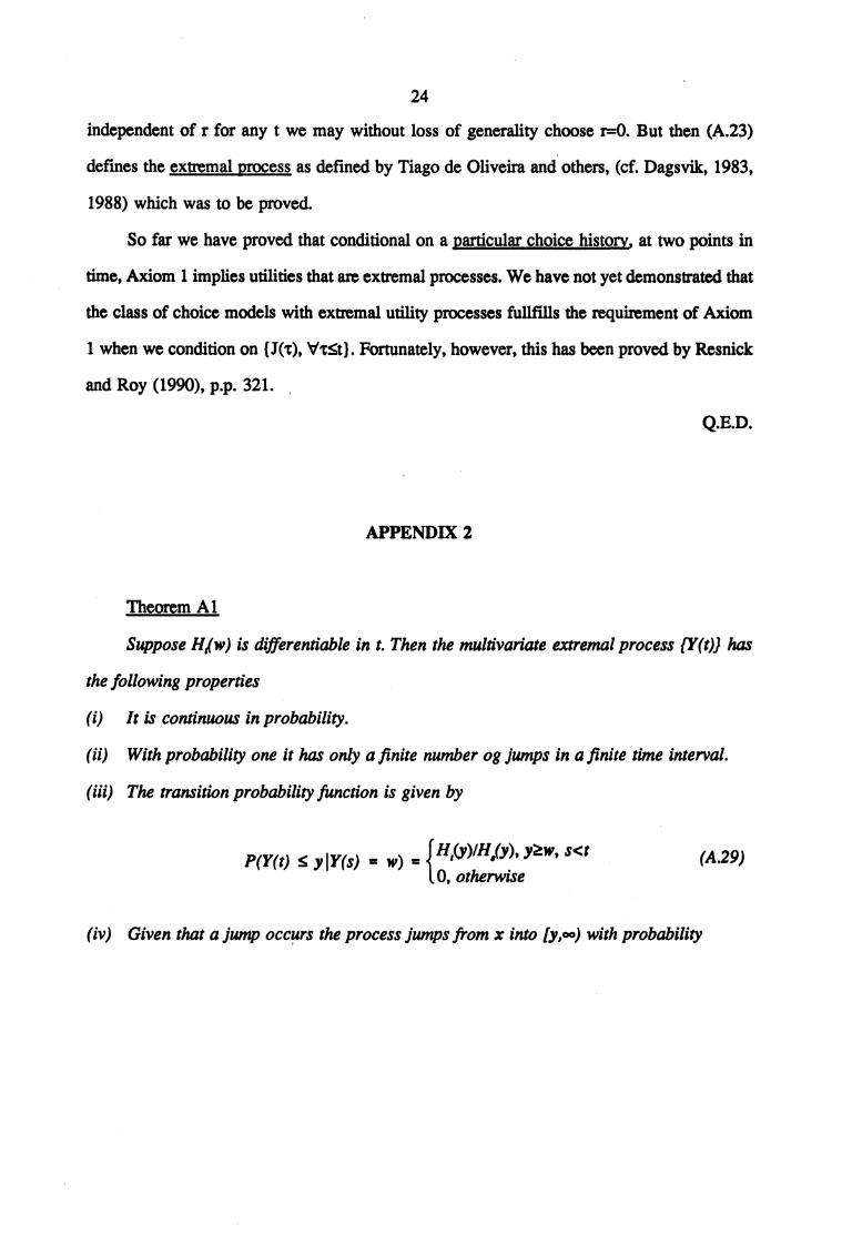
Theorem A l

Suppose Hi(w) is differentiable in t. Then the multivariate extrema! process OW)) has

the following properties

(i) It is continuous in probability.

(ii) With probability one it has only a finite number og jumps in a finite time interval.

(iii) The transition probability function is given by

11,(y)IH (y), jtw, s<tP(Y(t) ylY(s) = w) =

0, otherwise(A.29)

(iv) Given that a jump occurs the process jumps from x into [y,00) with probability

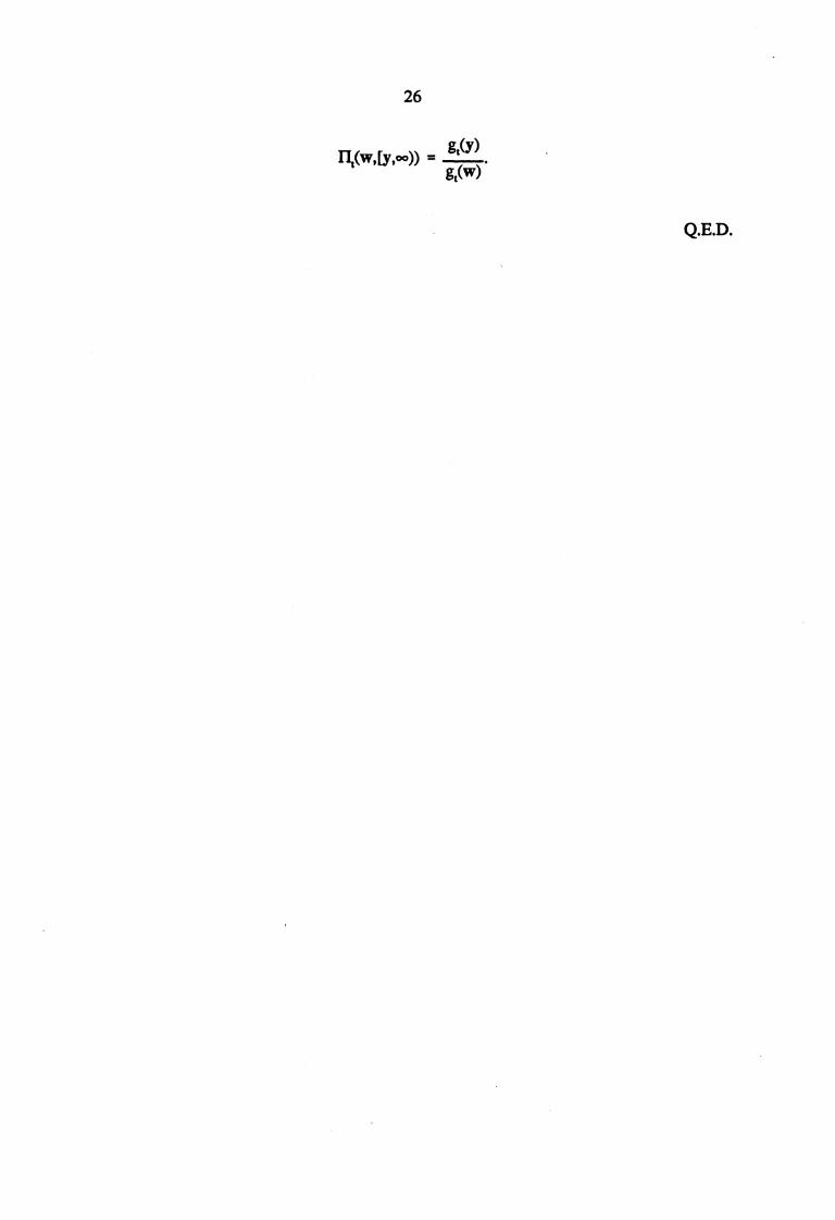
25

{g(Y)y>w11(w,fy,c0)) g(w)

0 if yw

(A.30)

where

g(y) = (A.31) at

Proof:

(i) This result is demonstrated by extending the proof by Resnick (1987) p. 182 to the

multivariate non-homogeneous case.

(ii) This is Theorem 1 in Dagsvik (1988).

Dagsvik (1988), p. 33 gives this result.

It thus only remains to prove (iv). From (iii) it follows that the intensity of a jump out

of state w is given by

lim(P(Y(t) > w IY(s) = w)/(t-s)) = g i(w).t-,S

Recall that IIt(w, [Y,°°)) is the probability that (Y(t)) jumps from w into [y ,00) given

that a jump occurs. Since {Y(t)} is a Markov process we have

lim(P(Y(t) > y IY(s) w)/(t-s)) = gt(w)fl(w,EY,00)).t-.11

But by (iii) we get

lim(P(Y(t) > y IY(s) = w)/(t-s)) = g t(y)

for pw and zero otherwise. Thus by combining the last two equations yields

26

ni(w,[3„-» = g1(y)

gt(w)

Q.E.D.

27

REFERENCES

Andersen, P.K., Hansen, L.S. and Keiding, N. (1991): "Non- and Semi-parametric Estimationof Transition Probabilities from Censored Observation of a Non-homogeneous MarkovProcess". Scand. J. Statist., 18, 153-167.

Chamberlain, G. (1985): "Heterogeneity, Omitted Variable Bias and Duration Dependence".In J.J. Heckman and B. Singer (eds.), Longitudinal analysis of labor market data,Cambridge University Press, London.

Dagsvik, J.K. (1983): "Discrete Dynamic Choice: An Extension of the Choice Models of Luceand Thurstone". J. Math. Psychology, 27, 1-43.

Dagsvik, J.K. (1988): "Markov Chains Generated by Maximizing Components of Multi-dimensional External Processes". Stochastic Proc. Appl., 28, 31-45.

Dagsvik, J.K. (1991): "How Large is the Class of Generalized Extreme Value Random UtilityModels?" Mimeo Central Bureau of Statistics, Oslo.

de Haan, L. (1984): "A Spectral Representation for Max-stable Processes". Ann. Probab., 12,1194-1204.

de Haan, L. and Resnick, S. (1977): "Limit Theory for Multivariate Sample Extremes". Z.Wahrscheinlichkeitsth., 40, 317-337.

Heckman, J.J. (1981): "Statistical Models for the Analysis of Discrete Panel Data". In C.F.Manski and D. McFadden (eds.), Structural analysis of discrete data. MIT Press,Cambridge.

Heckman, J.J. (1991): "Identifying the Hand of the Past: Distinguishing State Dependencefrom Heterogeneity". Am. Econ. Rev., 81, 75-79.

Kawata, T. (1972): "Fourier analysis in probability theory". Academic Press, New. York.

McFadden, D. (1981): "Probabilistic Theories of Choice". In C.F. Manski and D. McFadden(eds.), Structural analysis of discrete data. MIT Press, Cambridge.

Resnick, S. (1987): "Extreme value, regular variation and point processes". Springer Verlag,New York.

Resnick, S. and Roy, R. (1990): "Multivariate Extremal Processes, Leader Processes andDynamic Choice Models". Adv. Appl. Prob., 22, 309-331.

Simon, H.A. (1988): "Rationality as Process and as Product of Thought". In D.E. Bell, H.Raiffa and A. Tversky (eds.), Decision making; descriptive, normative, and prescriptive interactions. Cambridge University Press, Cambridge.

28

Thurstone, L. L. (1927): "A Law of Comparative Judgment". Psychological Rev., 34, 272-286.

Tiago de Oliveira, J. (1973): "An Extreme Markovian Stationary Process". Proceedings of thefourth conference in probability theory, Acad. Romania, Brasov, pp. 217-225.

29

ISSUED IN THE SERIES DISCUSSION PAPER

No. 1 I. Aslaksen and O. Bjerkholt (1985):Certainty Equivalence Procedures in theMacroeconomic Planning of an Oil Eco-nomy.

No. 3 E. Bjorn (1985): On the Prediction ofPopulation Totals from Sample surveysBased on Rotating Panels.

No. 4 P. Frenger (1985): A Short Run Dyna-mic Equilibrium Model of the NorwegianProduction Sectors.

No. 5 I. Aslaksen and O. Bjerkholt (1985):Certainty Equivalence Procedures in De-cision-Making under Uncertainty: AnEmpirical Application.

No. 6 E. Bien (1985): Depreciation Profilesand the User Cost of Capital.

No. 7 P. Frenger (1985): A Directional ShadowElasticity of Substitution.

No. 8 S. Longva, L. Lorentsen and Ø. Olsen(1985): The Multi-Sectoral Model MSG-4, Formal Structure and Empirical Cha-racteristics.

No. 9 J. Fagerberg and G. Sollie (1985): TheMethod of Constant Market Shares Revi-sited.

No. 10 E. Bjorn (1985): Specification of Con-sumer Demand Models with StochasticElements in the Utility Function and thefirst Order Conditions.

No. 14 R. Aaberge (1986): On the Problem ofMeasuring Inequality.

No. 15 A.-M. Jensen and T. Schweder (1986):The Engine of Fertility - Influenced byInterbirth Employment.

No. 16 E. Mown (1986): Energy Price Changes,and Induced Scrapping and Revaluationof Capital - A Putty-Clay Model.

No. 17 E. Bjorn and P. Frenger (1986): Ex-pectations, Substitution, and Scrapping ina Putty-Clay Model.

No. 18 R. Bergan, Å. Cappelen, S. Longva andN.M. Stolen (1986): MODAG A - AMedium Term Annual MacroeconomicModel of the Norwegian Economy.

No. 19 E. Bjorn and H. Olsen (1986): A Genera-lized Single Equation Error CorrectionModel and its Application to QuarterlyData.

No. 20 KR. Alfsen, DA. Hanson and S. Gloms-rod (1986): Direct and Indirect Effects ofreducing 502 Emissions: ExperimentalCalculations of the MSG-4E Model.

No. 21 IX. Dagsvik (1987): Econometric Ana-lysis of Labor Supply in a Life CycleContext with Uncertainty.

No. 22 KA. Brekke, E. Gjelsvik and B.H. Vatne(1987): A Dynamic Supply Side GameApplied to the European Gas Market.

No. 11 E. Bjorn, E. HolmOy and Ø. Olsen

No. 2.3 S. Bartlett, JX. Dagsvik, Ø. Olsen and S.(1985): Gross and Net Capital, Produc- StrOm (1987): Fuel Choice and the De-tivity and the fonn of the Survival Func- mand for Natural Gas in Western Euro-tion. Some Norwegian Evidence. pean Households.

No. 12 JX. Dagsvik (1985): Markov ChainsGenerated by Maximizing Components ofMultidimensional Extremal Processes.

No. 13 E. BiOrn, M. Jensen and M. Reytnert(1985): KVARTS - A Quarterly Model ofthe Norwegian Economy.

No. 24 J.K. Dagsvik and R. Aaberge (1987):Stochastic Properties and FunctionalForms of Life Cycle Models for Transit-ions into and out of Employment.

No. 25 T..I. Klette (1987): Taxing or Subsidisingan Exporting Industry.

30

No. 26 K.J. Berger, O. Bjerkholt and Ø. Olsen No. 38 T.J. Klette (1988): The Norwegian Alu-(1987): What are the Options for non- minium Industry, Electricity prices andOPEC Countries. Welfare, 1988.

No. 39 I. Aslaksen, O. Bjerkholt and KA. Brekke(1988): Optimal Sequencing of Hydro-electric and Thermal Power Generationunder Energy Price Uncertainty andDemand Fluctuations, 1988.

No. 40 O. Bjerkholt and KA. Brekke (1988):Optimal Starting and Stopping Rules forResource Depletion when Price is Exo-genous and Stochastic, 1988.

No. 41 J. Aasness, E. BiOrn and T. Skjerpen(1988): Engel Functions, Panel Data andLatent Variables, 1988.

No. 42 R. Aaberge, Ø. Kravdal and T. Wennemo(1989): Unobserved Heterogeneity inModels of Marriage Dissolution, 1989.

No. 43 KA. Mork, H.T. Mysen and Ø. Olsen(1989): Business Cycles and Oil PriceFluctuations: Some evidence for sixOECD countries. 1989.

No. 44 B. Bye, T. Bye and L. Lorentsen (1989):SIMEN. Studies of Industry, Environ-ment and Energy towards 2000, 1989.

No. 45 0. Bjerkholt, E. Gjelsvik and Ø. Olsen(1989): Gas Trade and Demand in North-west Europe: Regulation, Bargaining andCompetition.

No. 46 L.S. Stamb01 and K.O. Sørensen (1989):Migration Analysis and Regional Popu-lation Projections, 1989.

No. 47 V. Christiansen (1990): A Note on theShort Run Versus Long Run WelfareGain from a Tax Reform, 1990.

No. 48 S. Glomsrød, H. Vennemo and T. John-sen (1990): Stabilization of emissions ofCO: A computable general equilibriumassessment, 1990.

No. 49 J. Aasness (1990): Properties of demandfunctions for linear consumption aggre-gates, 1990.

No. 50 J.G. de Leon (1990): Empirical EDAModels to Fit and Project Time Series ofAge-Specific Mortality Rates, 1990.

No. 27 A. Aaheim (1987): Depletion of LargeGas Fields with Thin Oil Layers andUncertain Stocks.

No. 28 JX. Dagsvik (1987): A Modification ofHeckman's Two Stage Estimation Proce-dure that is Applicable when the BudgetSet is Convex.

No. 29 K. Berger, A. Cappelen and I. Svendsen(1988): Investment Booms in an OilEconomy The Norwegian Case.

No. 30 A. Rygh Swensen (1988): EstimatingChange in a Proportion by CombiningMeasurements from a True and a FallibleClassifier.

No. 31 J.K. Dagsvik (1988): The ContinuousGeneralized Extreme Value Model withSpecial Reference to Static Models ofLabor Supply.

No. 32 K. Berger, M. Hoel, S. Holden and Ø.Olsen (1988): The Oil Market as anOligopoly.

No. 33 IAX. Anderson, J.K. Dagsvik, S. StrOmand T. Wennemo (1988): Non-ConvexBudget Set, Hours Restrictions and LaborSupply in Sweden.

No. 34 E. Holmøy and Ø. Olsen (1988): A Noteon Myopic Decision Rules in the Neo-classical Theory of Producer Behaviour,1988.

No. 35 E. Biørn and H. Olsen (1988): Production- Demand Adjustment in NorwegianManufacturing: A Quarterly Error Cor-rection Model, 1988.

No. 36 J.K. Dagsvik and S. Strom (1988): ALabor Supply Model for Married Coupleswith Non-Convex Budget Sets and LatentRadom' g, 1988.

No. 37 T. Skoglund and A. Stokka (1988): Prob-lems of Linking Single-Region and Mul-tiregional Economic Models, 1988.

31

No. 51 LG. de Leon (1990): Recent Develop- No. 64 A. Brendemoen and H. Vennemo (1991):ments in Parity Progression Intensities in Aclimate convention and the Norwegian

Norway. An Analysis Based on Popu- economy: A CGE assessment.lation Register Data.

No. 52 R. Aaberge and T. Wennemo (1990):Non-Stationary Inflow and Duration ofUnemployment.

No. 53 R. Aaberge, JX. Dagsvik and S. StrOm(1990): Labor Supply, Income Distri-bution and Excess Burden of PersonalIncome Taxation in Sweden.

No. 54 R. Aaberge, JX. Dagsvik and S. &Om(1990): Labor Supply, Income Distri-bution and Excess Burden of PersonalIncome Taxation in Norway.

No. 65 K. A. Brekke (1991): Net National Pro-duct as a Welfare Indicator.

No. 66 E. Bowitz and E. Storm (1991): Willrestrictive demand policy improve publicsector balance?

No. 67 A. Cappelen (1991): MODAG. A Medi-um Term Macroeconomic Model of theNorwegian Economy.

No. 68 B. Bye (1992): Modelling Consumers'Energy Demand.

No. 69 K. H. Alfsen, A. Brendemoen and S.No. 55 H. Vennemo (1990): Optimal Taxation in

Glomsrod (1992): Benefits of Climate

Applied General Equilibrium Models

Policies: Some Tentative Calculations.Adopting the Annington Assumption.

No. 56 NM. StOlen (1990): Is there a NAIRU inNorway?

No. 57 A. Cappelen (1991): MacroeconomicModelling: The Norwegian Experience.

No. 58 J. Dagsvik and R. Aaberge (1991):Household Production, Consumption andTime Allocation in Peru.

No. 59 R. Aaberge and J. Dagsvik (1991): In-equality in Distribution of Hours of Workand Consumption in Peru.

No. 60 Ti. Klette (1991): On the Importance ofR&D and Ownership for ProductivityGrowth. Evidence from NorwegianMicro-Data 1976-85.

No. 61 K.H. Alfsen (1991): Use of macroecono-mic models in analysis of environmentalproblems in Norway and consequencesfor environmental statistics.

No. 62 H. Vennemo (1991): An Applied GeneralEquilibrium Assessment of the MarginalCost of Public Funds in Norway.

No. 63 H. Vennemo (1991): The marginal cost ofpublic funds: A comment on the litera-ture.

No. 70 R. Aaberge, Xiaojie Chen, Jing Li andXuezeng Li (1992): The structure ofeconomic inequality among householdsliving in urban Sichuan and Liaoning,1990.

No. 71 K.!!. Alfsen, KA. Brekke, F. Brunvoll, H.Lurds, K. Nyborg and H.W. Steb0 (1992):Environmental Indicators.

No. 72 B. Bye and E. Holm*, (1992): Dynamicequilibrium adjustments to a terms oftrade disturbance

No. 73 O. Aukrust (1992): The Scandinaviancontribution to national accounting

No. 74 J. Aasness, E, Eide and T. Skjerpen(1992): A criminometric study usingpanel data and latent variables (will beissued later)

No. 75 R. Aaberge and Xuezeng Li (1992): Thetrend in income inequality in urbanSichuan and Liaoning, 1986-1990

No. 76 J.K. Dagsvik and Steinar StrOm (1992):Labor sypply with non-convex budgetsets, hours restriction and non-pecuniaryjob-attributes

No. 77 J.K. Dagsvik (1992): Intertemporal dis-crete choice, random tastes and func-tional form